penelitian operasional iaeunike.lecture.ub.ac.id/files/2012/11/pertemuan-12-or.pdf ·...
TRANSCRIPT

PENELITIAN OPERASIONAL I
(TIN 4109)

Lecture 12
INTEGER PROGRAMMING

Lecture 12
• Outline: – Integer Programming: Binary
• References: – Frederick Hillier and Gerald J. Lieberman. Introduction to
Operations Research. 7th ed. The McGraw-Hill Companies, Inc, 2001.
– Hamdy A. Taha. Operations Research: An Introduction. 8th Edition. Prentice-Hall, Inc, 2007.
– Winston, Wayne L. Operations Research: Applications and Algorithms. 3rd edition. Wadsworth Inc.1994.
– Hartanto, Dody. Lecture PPT: Pemodelan dalam Pemrogaman Linier Integer (Modeling in Integer Linear Programming). ITS. 2012

BINARY INTEGER PROGRAMMING INTEGER PROGRAMMING

Algoritma Branch and Bound untuk BILP (Binary Integer Linear
Programming)
Dody Hartanto
Maksimasi
Z = 9x1 + 5x2 + 6x3 + 4x4
pembatas:
6x1 + 3x2 + 5x3 + 2x4 10
x3 + x4 1
-x1 + x3 0
-x2 + x4 0
x1, x2, x3, x4 = {0, 1}

Algoritma Branch and Bound untuk BILP
Dody Hartanto
Dody Hartanto
• Masalah asli (original problem) diselesaikan dengan mengabaikan batasan yang mengharuskan variabel keputusan bernilai integer (ILP relaksasi).
• Solusi ILP relaksasi masalah asli memiliki satu variabel keputusan yang tidak bernilai bulat yaitu X1 sehingga perlu dilakukan pencabangan.
Algoritma Branch and Bound untuk BILP(1)
Dody Hartanto
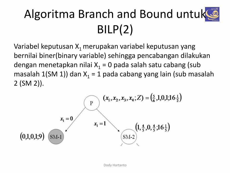
Variabel keputusan X1 merupakan variabel keputusan yang bernilai biner(binary variable) sehingga pencabangan dilakukan dengan menetapkan nilai X1 = 0 pada salah satu cabang (sub masalah 1(SM 1)) dan X1 = 1 pada cabang yang lain (sub masalah 2 (SM 2)).
Algoritma Branch and Bound untuk BILP(2)
Dody Hartanto
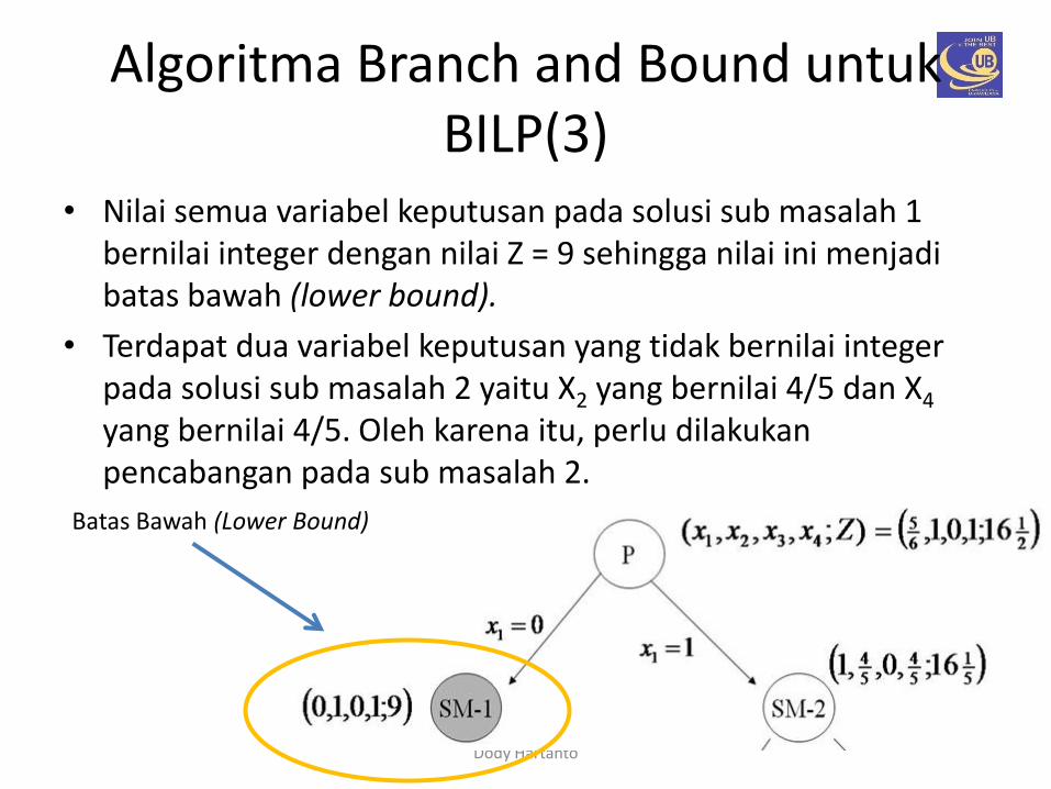
• Nilai semua variabel keputusan pada solusi sub masalah 1 bernilai integer dengan nilai Z = 9 sehingga nilai ini menjadi batas bawah (lower bound).
• Terdapat dua variabel keputusan yang tidak bernilai integer pada solusi sub masalah 2 yaitu X2 yang bernilai 4/5 dan X4 yang bernilai 4/5. Oleh karena itu, perlu dilakukan pencabangan pada sub masalah 2.
Batas Bawah (Lower Bound)
Algoritma Branch and Bound untuk BILP(3)

Dody Hartanto
Pencabangan pada sub masalah 2 dilakukan dengan menetapkan X2 = 0 pada salah satu cabang (sub masalah 3(SM 3)) dan X2 = 1 pada cabang yang lain (sub masalah 4 (SM 4)).
Algoritma Branch and Bound untuk BILP(4)

Dody Hartanto
• Tidak semua variabel keputusan pada solusi sub masalah 3 bernilai integer demikian pula dengan solusi pada sub masalah 4. Oleh karena itu perlu dilakukan pencabangan pada kedua sub masalah(sub masalah 3 dan sub masalah 4).
karena nilai Z pada sub masalah 4 yang bernilai 16 adalah lebih besar jika dibandingkan dengan nilai Z pada sub masalah 3 yang bernilai 13,8 maka pencabangan dilakukan terlebih dahulu pada sub masalah 4.
Algoritma Branch and Bound untuk BILP(5)

Dody Hartanto
Pencabangan pada sub masalah 4 dilakukan dengan menetapkan X4 = 0 pada salah satu cabang (sub masalah 5(SM 5)) dan X4 = 1 pada cabang yang lain (sub masalah 6 (SM 6)). Semua variabel keputusan pada solusi sub masalah 5 bernilai integer dengan nilai fungsi tujuan Z= 14.
Algoritma Branch and Bound untuk BILP(6)

Dody Hartanto
Nilai Z pada sub masalah 5 lebih besar jika dibandingkan dengan batas bawah (lower bound) yang sekarang(solusi dari sub masalah 1) sehingga batas bawah yang semula bernilai 9 diubah menjadi 14
Batas Bawah (Lower Bound) yang lama
Batas Bawah (Lower Bound) yang Baru
Algoritma Branch and Bound untuk BILP(7)
Dody Hartanto
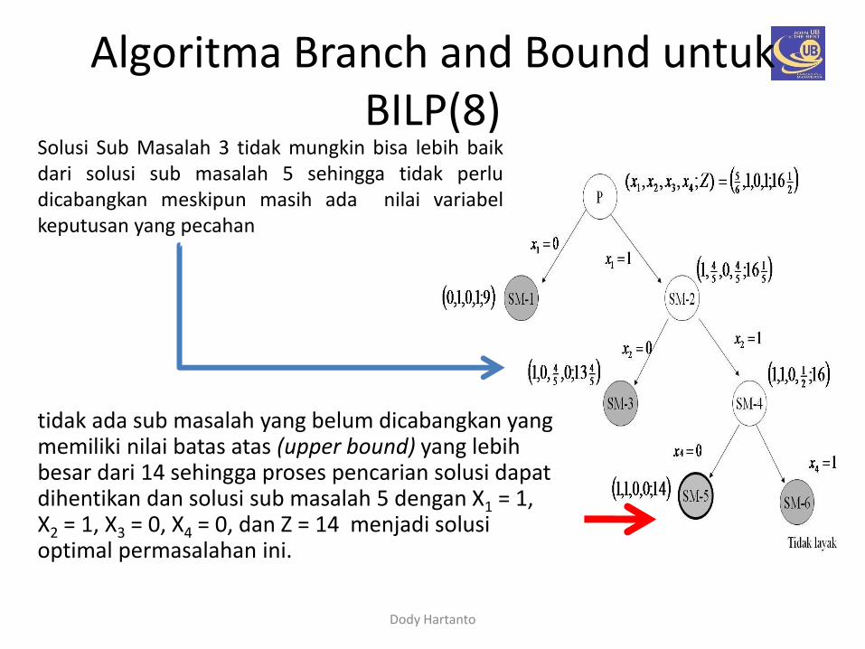
tidak ada sub masalah yang belum dicabangkan yang memiliki nilai batas atas (upper bound) yang lebih besar dari 14 sehingga proses pencarian solusi dapat dihentikan dan solusi sub masalah 5 dengan X1 = 1, X2 = 1, X3 = 0, X4 = 0, dan Z = 14 menjadi solusi optimal permasalahan ini.
Solusi Sub Masalah 3 tidak mungkin bisa lebih baik dari solusi sub masalah 5 sehingga tidak perlu dicabangkan meskipun masih ada nilai variabel keputusan yang pecahan
Algoritma Branch and Bound untuk BILP(8)

LP dan ILP dengan Software
• TUGAS KELOMPOK: – Temukan satu permasalahan yang memerlukan solusi
optimal (permasalahan LP: 1 dan ILP: 1). Buat formulasinya. Selesaikan dengan menggunakan software: LINDO/LINGO dan Solver.
– Isi laporan: • Deskripsi Permasalahan • Formulasi • Langkah-langkah pengerjaan dengan software • Solusi dan Kesimpulan
– Format laporan: • PPT

Lecture 13
TRANSPORTATION

Lecture 13
• Outline:
– Transportation: starting basic feasible solution
• References:
– Frederick Hillier and Gerald J. Lieberman. Introduction to Operations Research. 7th ed. The McGraw-Hill Companies, Inc, 2001.
– Hamdy A. Taha. Operations Research: An Introduction. 8th Edition. Prentice-Hall, Inc, 2007.

Transportation

Description A transportation problem basically deals with the problem,
which aims to find the best way to fulfill the demand of n
demand points using the capacities of m supply points.
1
2
3
1
2
c11
c12
c13
c21 c22
c23
d1
d2
d3
s1
s2
SOURCES DESTINATIONS

Transportation Problem • LP Formulation
The linear programming formulation in terms of the amounts shipped from the origins to the destinations, xij, can be written as:
Min SScijxij i j s.t. Sxij < si for each source i j Sxij >= dj for each destination j i xij > 0 for all i and j

Transportation Problem
• LP Formulation Special Cases
The following special-case modifications to the linear programming formulation can be made: – Minimum shipping guarantees from i to j:
xij > Lij
– Maximum route capacity from i to j:
xij < Lij
– Unacceptable routes:
delete the variable

Example: BBC
Building Brick Company (BBC) has orders for 80 tons of
bricks at three suburban locations as follows: Northwood -- 25
tons, Westwood -- 45 tons, and Eastwood -- 10 tons. BBC has
two plants, each of which can produce 50 tons per week.
How should end of week shipments be made to fill the
above orders given the following delivery cost per ton:
Northwood Westwood Eastwood
Plant 1 24 30 40
Plant 2 30 40 42

Example: BBC
• LP Formulation
– Decision Variables Defined
xij = amount shipped from plant i to suburb j
where i = 1 (Plant 1) and 2 (Plant 2)
j = 1 (Northwood), 2 (Westwood),
and 3 (Eastwood)

Example: BBC • LP Formulation
– Objective Function Minimize total shipping cost per week:
Min 24x11 + 30x12 + 40x13 + 30x21 + 40x22 + 42x23
– Constraints s.t. x11 + x12 + x13 < 50 (Plant 1 capacity)
x21 + x22 + x23 < 50 (Plant 2 capacity)
x11 + x21 >= 25 (Northwood demand)
x12 + x22 >= 45 (Westwood demand)
x13 + x23 >= 10 (Eastwood demand)
all xij > 0 (Non-negativity)

Exercise…. Powerco has three electric power plants that supply the electric
needs of four cities.
• The associated supply of each plant and demand of each city is given in the table as follows:
• The cost of sending 1 million kwh of electricity from a plant to a city depends on the distance the electricity must travel.
From To
City 1 City 2 City 3 City 4 Supply
(Million kwh)
Plant 1 $8 $6 $10 $9 35
Plant 2 $9 $12 $13 $7 50
Plant 3 $14 $9 $16 $5 40
Demand
(Million kwh)
45 20 30 30

Solution 1. Decision Variable: Since we have to determine how much electricity is sent from each
plant to each city; Xij = Amount of electricity produced at plant i and sent to city j X14 = Amount of electricity produced at plant 1 and sent to city 4 2. Objective Function: Since we want to minimize the total cost of shipping from plants to
cities; Minimize Z = 8X11+6X12+10X13+9X14+9X21+12X22+13X23+7X24
+14X31+9X32+16X33+5X34

3. Supply Constraints
X11+X12+X13+X14 <= 35
X21+X22+X23+X24 <= 50
X31+X32+X33+X34 <= 40
4. Demand Constraints
Solution
X11+X21+X31 >= 45
X12+X22+X32 >= 20
X13+X23+X33 >= 30
X14+X24+X34 >= 30
Since each supply point has a
limited production capacity;
Since each supply point has a
limited production capacity;
5. Sign Constraints
Xij >= 0 (i= 1,2,3; j= 1,2,3,4)

LP Formulation of Powerco’s Problem
Min Z = 8X11+6X12+10X13+9X14+9X21+12X22+13X23+7X24
+14X31+9X32+16X33+5X34
S.T.: X11+X12+X13+X14 <= 35 (Supply Constraints)
X21+X22+X23+X24 <= 50
X31+X32+X33+X34 <= 40
X11+X21+X31 >= 45 (Demand Constraints)
X12+X22+X32 >= 20
X13+X23+X33 >= 30
X14+X24+X34 >= 30
Xij >= 0 (i= 1,2,3; j= 1,2,3,4)
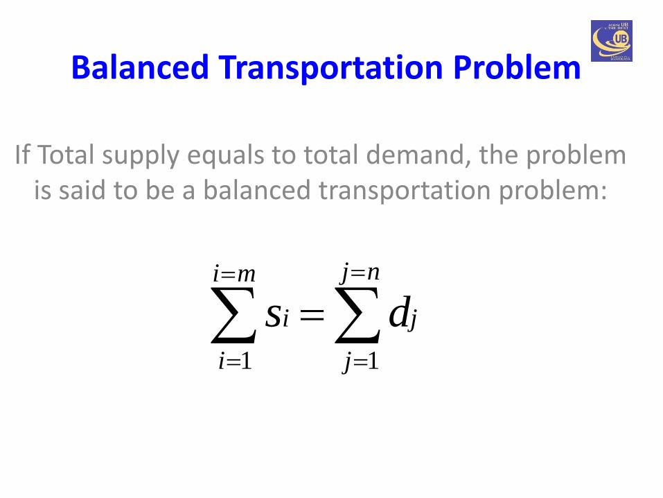
Balanced Transportation Problem
If Total supply equals to total demand, the problem is said to be a balanced transportation problem:
nj
j
j
mi
i
i ds11

Finding Basic Feasible Solution for Transportation Problem
Unlike other Linear Programming problems,
a balanced TP with m supply points and n demand points is
easier to solve, although it has m + n equality constraints.
The reason for that is, if a set of decision variables (xij’s)
satisfy all but one constraint, the values for xij’s will satisfy
that remaining constraint automatically.

Methods to find the BFS for a balanced Transportation Problem
There are three basic methods:
1. North West Corner Method
2. Minimum Cost Method
3. Vogel’s Method

1. Northwest Corner Method
To find the bfs by the NWC method:
Begin in the upper left (northwest) corner of the transportation tableau and set x11 as large as possible (here the limitations for setting x11 to a larger number, will be the demand of demand point 1 and the supply of supply point 1. Your x11 value can not be greater than minimum of this 2 values).

According to the explanations in the previous slide we can set x11=3 (meaning demand of demand point 1 is satisfied
by supply point 1).
5
6
2
3 5 2 3
3 2
6
2
X 5 2 3

After we check the east and south cells, we saw that we can go east (meaning supply point 1 still has capacity to fulfill some demand).
3 2 X
6
2
X 3 2 3
3 2 X
3 3
2
X X 2 3

After applying the same procedure, we saw that we can go south this time (meaning demand point 2 needs more supply
by supply point 2).
3 2 X
3 2 1
2
X X X 3
3 2 X
3 2 1 X
2
X X X 2

Finally, we will have the following bfs, which is: x11=3, x12=2, x22=3, x23=2, x24=1, x34=2
3 2 X
3 2 1 X
2 X
X X X X

2. Minimum Cost Method
The Northwest Corner Method dos not utilize shipping costs.
It can yield an initial BFS easily but the total shipping cost may
be very high.
The minimum cost method uses shipping costs in order come
up with a BFS that has a lower cost.

1. First, We look for the cell with the minimum cost of shipping in
the overall transportation tableau.
2. We should cross out row i and column j and reduce the supply
or demand of the noncrossed-out row or column by the value
of Xij.
3. Then we will choose the cell with the minimum cost of shipping
from the cells that do not lie in a crossed-out row or column
and we will repeat the procedure.
2. Minimum Cost Method (Cont’d)
The Steps:

An example for Minimum Cost Method Step 1: Select the cell with minimum cost.
2 3 5 6
2 1 3 5
3 8 4 6
5
10
15
12 8 4 6

Step 2: Cross-out column 2
2 3 5 6
2 1 3 5
8
3 8 4 6
12 X 4 6
5
2
15

Step 3: Find the new cell with minimum shipping cost and cross-out row 2
2 3 5 6
2 1 3 5
2 8
3 8 4 6
5
X
15
10 X 4 6

Step 4: Find the new cell with minimum shipping cost and cross-out row 1
2 3 5 6
5
2 1 3 5
2 8
3 8 4 6
X
X
15
5 X 4 6

Step 5: Find the new cell with minimum shipping cost and cross-out column 1
2 3 5 6
5
2 1 3 5
2 8
3 8 4 6
5
X
X
10
X X 4 6

Step 6: Find the new cell with minimum shipping cost and cross-out column 3
2 3 5 6
5
2 1 3 5
2 8
3 8 4 6
5 4
X
X
6
X X X 6

Step 7: Finally assign 6 to last cell. The bfs is found as: X11=5, X21=2, X22=8, X31=5, X33=4 and X34=6
2 3 5 6
5
2 1 3 5
2 8
3 8 4 6
5 4 6
X
X
X
X X X X

3. Vogel’s Method
1. Begin with computing each row and column a penalty. The
penalty will be equal to the difference between the two smallest
shipping costs in the row or column.
2. Identify the row or column with the largest penalty.
3. Find the first basic variable which has the smallest shipping cost
in that row or column.
4. Then assign the highest possible value to that variable, and cross-
out the row or column as in the previous methods. Compute new
penalties and use the same procedure.

An example for Vogel’s Method Step 1: Compute the penalties.
Supply Row Penalty
6 7 8
15 80 78
Demand
Column Penalty 15-6=9 80-7=73 78-8=70
7-6=1
78-15=63
15 5 5
10
15

Step 2: Identify the largest penalty and assign the highest possible value to the variable.
Supply Row Penalty
6 7 8
5
15 80 78
Demand
Column Penalty 15-6=9 _ 78-8=70
8-6=2
78-15=63
15 X 5
5
15

Step 3: Identify the largest penalty and assign the highest possible value to the variable.
Supply Row Penalty
6 7 8
5 5
15 80 78
Demand
Column Penalty 15-6=9 _ _
_
_
15 X X
0
15
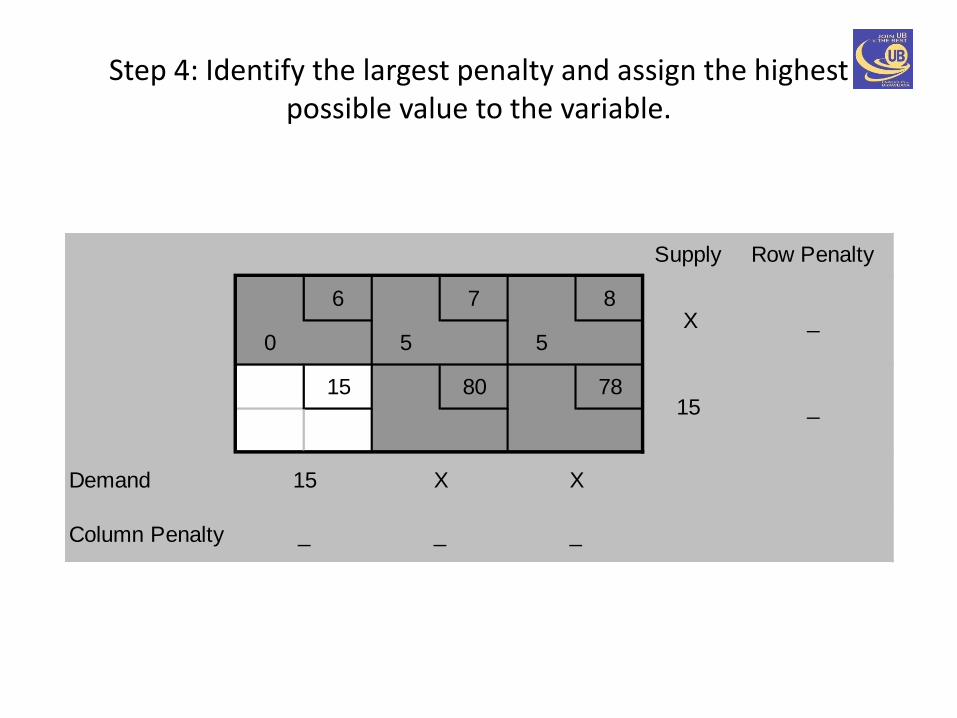
Step 4: Identify the largest penalty and assign the highest possible value to the variable.
Supply Row Penalty
6 7 8
0 5 5
15 80 78
Demand
Column Penalty _ _ _
_
_
15 X X
X
15

Step 5: Finally the bfs is found as X11=0, X12=5, X13=5, and X21=15
Supply Row Penalty
6 7 8
0 5 5
15 80 78
15
Demand
Column Penalty _ _ _
_
_
X X X
X
X

Exercise
Bazaraa Chapter 10:
Solve the following transportation problem:
1 2 3 si
1 5 4 1 3
2 1 7 5 7
dj 2 5 3
Origin
Destination
cij matrix

Exercise Bazaraa Chapter 10:
1 2 3 4 si
1 7 2 -1 0 10
2 4 3 2 3 30
3 2 1 3 4 25
dj 10 15 25 15
cij matrix
Solve the following transportation problem:

Lecture 14 – Preparation
• Materi:
– Transportasi: Optimum Solution
