pendulum project - university of notre damejszczud1/pendulum project report.docx · web...

University of Notre dame

Pendulum Project

AME 30315

Joshua SzczudlakFiras Fasheh

5/2/2012

For me, I am driven by two main philosophies, know more today about the world than I knew yesterday. And lessen the suffering of others. You'd be surprised how far that gets you.

- Neil deGrasse Tyson

University of Notre Dame AME 30315 Pendulum Project

Abstract

The purpose of this project was to design a controller that stabilizes an inverted pendulum. The first step in designing the controller was to identify the system. Through the process of system identification it was found that ωn=6.28Hz and ξ=0.055. Next, a transfer function was derived for the system using the governing equations of motion. This transfer function was found for an output position, R in terms of an input torque, T . Additionally, lead and lag compensators were created to help stabilize the system. Two lead-lag compensators were designed. One controller used the assigned parameters of ξ=0.32 and a lag gain of 92. The other controller was designed for optimal performance including a half second rise time, quick settling time, and small stead-state error. These parameters were evaluated using root locus plots and the used of Simulink to predict performance.

1 | P a g e


Table of Contents

1 System..........................................................................................................41.1 System Identification.......................................................................4

1.1.1 Design Parameters...................................................................52 Control Design.............................................................................................5

2.1 Continuous Transfer Function.........................................................52.1.1 Hanging Pendulum..................................................................52.1.2 Inverted Pendulum...................................................................6

2.2 Design Parameters..........................................................................72.3 Lead Control....................................................................................7

2.3.1 Design......................................................................................82.3.2 Lead Calculation......................................................................8

2.4 Lag Control......................................................................................92.4.1 Design......................................................................................92.4.2 Lag Calculation........................................................................9

2.5 Discrete-time Transfer Function...................................................102.5.1 Conversion to Discrete-time..................................................10

3 Controller Implementation.........................................................................103.1 Controller Implementation............................................................10

3.1.1 Non-dimensionalization.........................................................103.1.2 Error Calculation...................................................................113.1.3 Transfer Function Implementation........................................11

5 System Evaluation......................................................................................115.1 Theoretical Modeling.....................................................................115.2 Transient Evaluation......................................................................12

5.2.1 Rise Time Evaluation.............................................................135.2.2 Overshoot Evaluation.............................................................13

5.3 Steady-State Evaluation................................................................136 System Verification....................................................................................14

6.1 Position Verification.......................................................................147 Conclusions................................................................................................15

Appendix A: Matlab CodeAppendix B: C CodeAppendix C: Discretization of Transfer FunctionAppendix D: Derivations of Transfer FunctionAppendix E: Lead Compensator CalculationsAppendix F: Iterations Table

List of TablesTable 1. Steady-state error in the controller at various desired angles.......14

2 | P a g e


List of FiguresFigure 1. Measured damped frequency response...........................................5Figure 2. Root locus of the hanging pendulum transfer function...................6Figure 3. Comparison of measured damped frequency response and derived transfer function.............................................................................................6Figure 3. Root locus of the inverted pendulum transfer function..................7Figure 4. Root locus with effect of the lead compensator..............................9Figure 5. Root locus of the transfer function with the lead-lag compensator.......................................................................................................................10Figure 6. Representative Simulink block diagram.......................................12Figure 7. Response predicted by Simulink...................................................12Figure 8. Response of pendulum..................................................................13Figure 9. Response of pendulum at angles of -30º to 30º.............................14

3 | P a g e


1 System

1.1 System IdentificationThe first step to designing a controller is to determine what sort of system you are dealing with and what parameters you need to model the system accurately. Determining the parameters to the pendulum system is fairly simple because when a step input is sent to the pendulum it responds in an easily understood sinusoidal manner. The parameters necessary for the modeling of the pendulum are ξ, the damping ratio, ωn, the natural frequency, and F a scale factor. A series of simple equations can be used to determine these expressions. The first equation can be used to find the damping ratio,

δ= ln( x2

x3)= −2 πξ

√1−ξ2 (1)

where δ is the logarithmic decrement, ξ is the damping ratio of the system, and x2 and x3 are the distance from the steady-state value of the second and third peaks respectively. This equation can be used to determine the damping ratio of the pendulum system.

Knowledge of the period and the damping ratio allows us to find the damped natural frequency of the system.

ωd=2πT (2)

where ωd is the damped natural frequency, and T is the period. Using the damped natural frequency and the damping ratio the natural frequency can be determined.

ωn=ωd

√1−ξ2 (3)

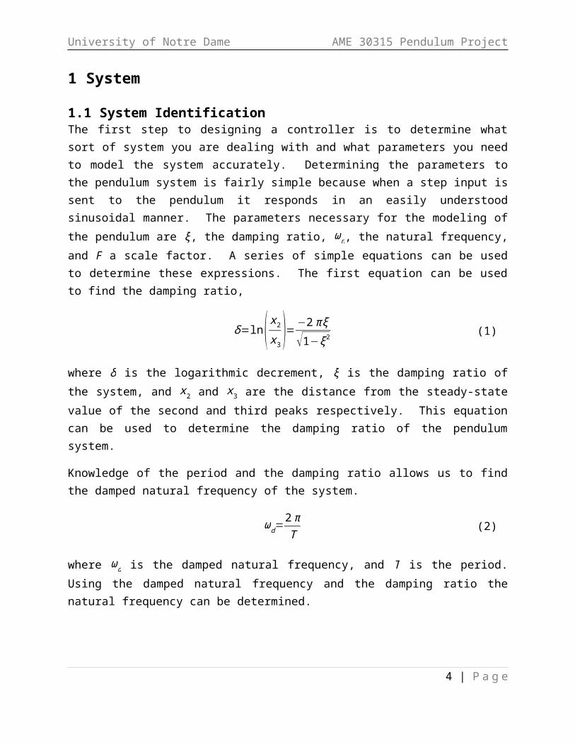
where ωn is the natural frequency. A final scale factor was determined by multiplying the steady-state value by the square of the natural frequency and dividing by the value of the applied torque. Figure 1 shows the damped frequency response of the pendulum.

4 | P a g e


0 1 2 3 4 5 6-100

-50

0

50

100

150

200

250

time [s]

posi

tion

[enc

onde

r cou

nts]

Figure 1. Measured damped frequency response

The parameters derived from this plot are outlined in section 1.1.1 Design Parameters.

1.1.1 Design ParametersThe design parameters were determined through the system identification process outlined above. The parameters used in the design of the pendulum controller were found by averaging data taken by testing multiple pendulums at various torques. Doing this ensured that any pendulum could be used with relative accuracy. This process yielded the following parameters: ωn was 6.28 Hz, ξ was 0.055, and the scale factor F was 37.2. Additional system identification plots can be found in the Matlab code in Appendix A.

2 Control Design

2.1 Continuous Transfer FunctionA transfer function in the continuous time domain was derived first for the hanging pendulum system. This system is then inverted for uses in the inverted pendulum system. The inverted pendulum transfer function is then discretized for use in the microcontroller.

2.1.1 Hanging PendulumThe transfer function of the pendulum is shown in the following equation,

5 | P a g e


T ( s )R (s )

= 1s2+2ξωn+ωn

2 (4)

where R is the input position error and T is the output torque. Appendix D shows the calculations necessary to obtain the transfer function for the hanging pendulum.

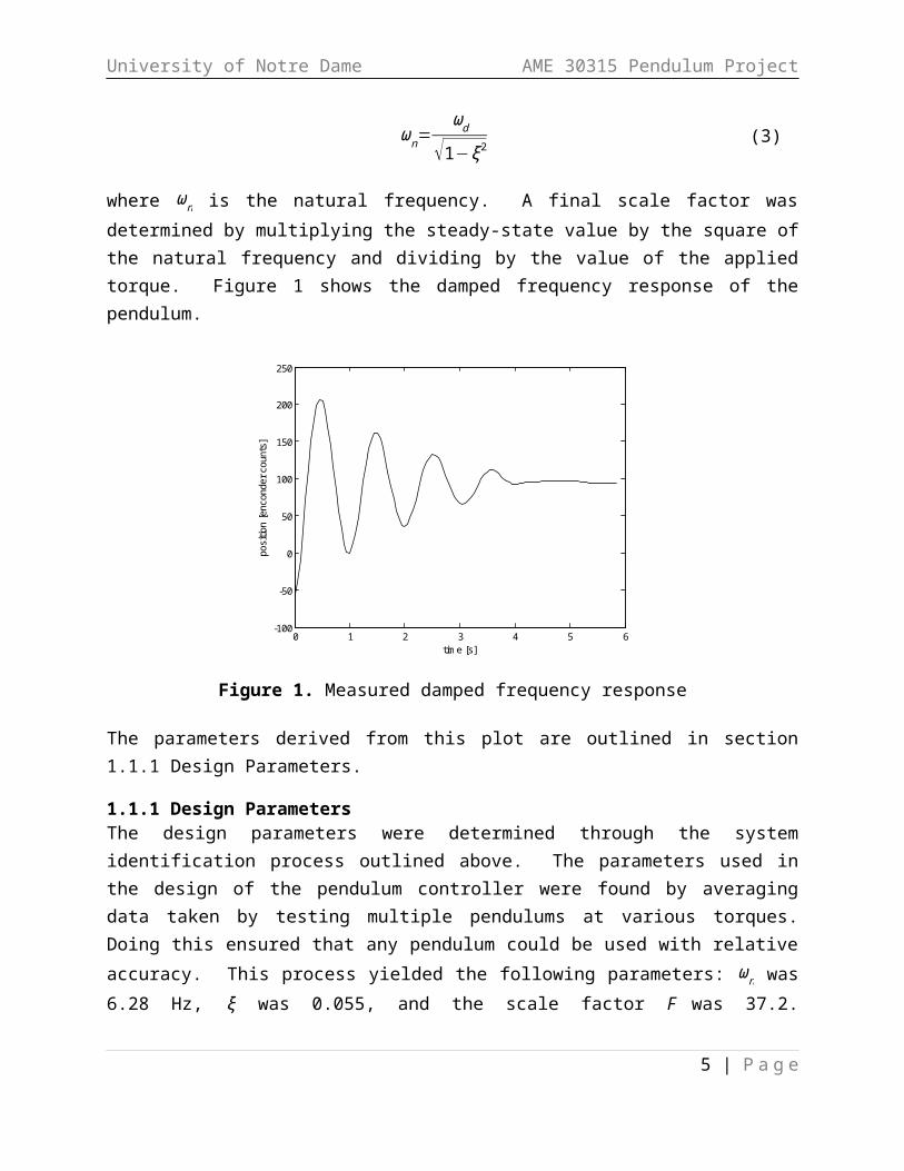
Figure 2 is the root locus plot of the hanging pendulum system.

-4 -3 -2 -1 0 1 2 3-30

-20

-10

0

10

20

30Root Locus

Real Axis (seconds-1)

Imag

inar

y Ax

is (s

econ

ds-1

)

Figure 2. Root locus of the hanging pendulum transfer function

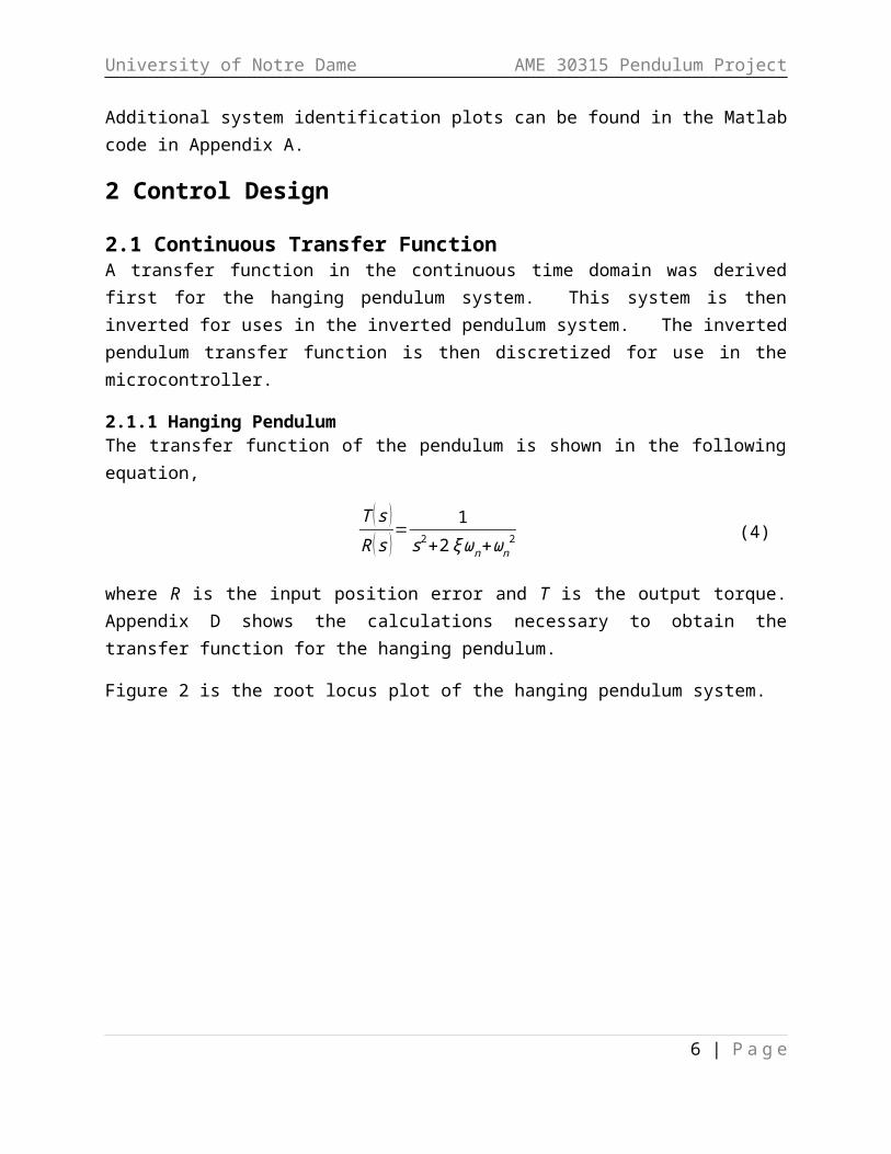
Figure 3 shows the measured response of the hanging pendulum system and the hanging pendulum transfer function after it has been subject to a step input. The similarity between the two helps to verify the accuracy of the model as well as the accuracy of the values obtained from the system identification.

6 | P a g e


Step Response

Time (seconds)

Ampl

itude

0 1 2 3 4 5 6 7 8-100

-50

0

50

100

150

200

250

Measured ResponseTheoretical Model

Figure 3. Comparison of measured damped frequency response and derived transfer function

2.1.2 Inverted PendulumAfter obtaining the transfer function for the hanging pendulum the transfer function for the inverted system is almost trivial. The difference is in a sign difference in the equations of motion. This transfer function is shown in the following equation,

T ( s)R (s )

= 1s2+2ξωn−ωn

2 (5)

The only difference between the two transfer functions is that the pendulum responds to the force of gravity. When the hanging pendulum is displaced in the positive direction, the gravitational force opposes it. However, in the inverted pendulum system the gravitational force works with displacement. This difference causes the sign change on the ωn2 term.

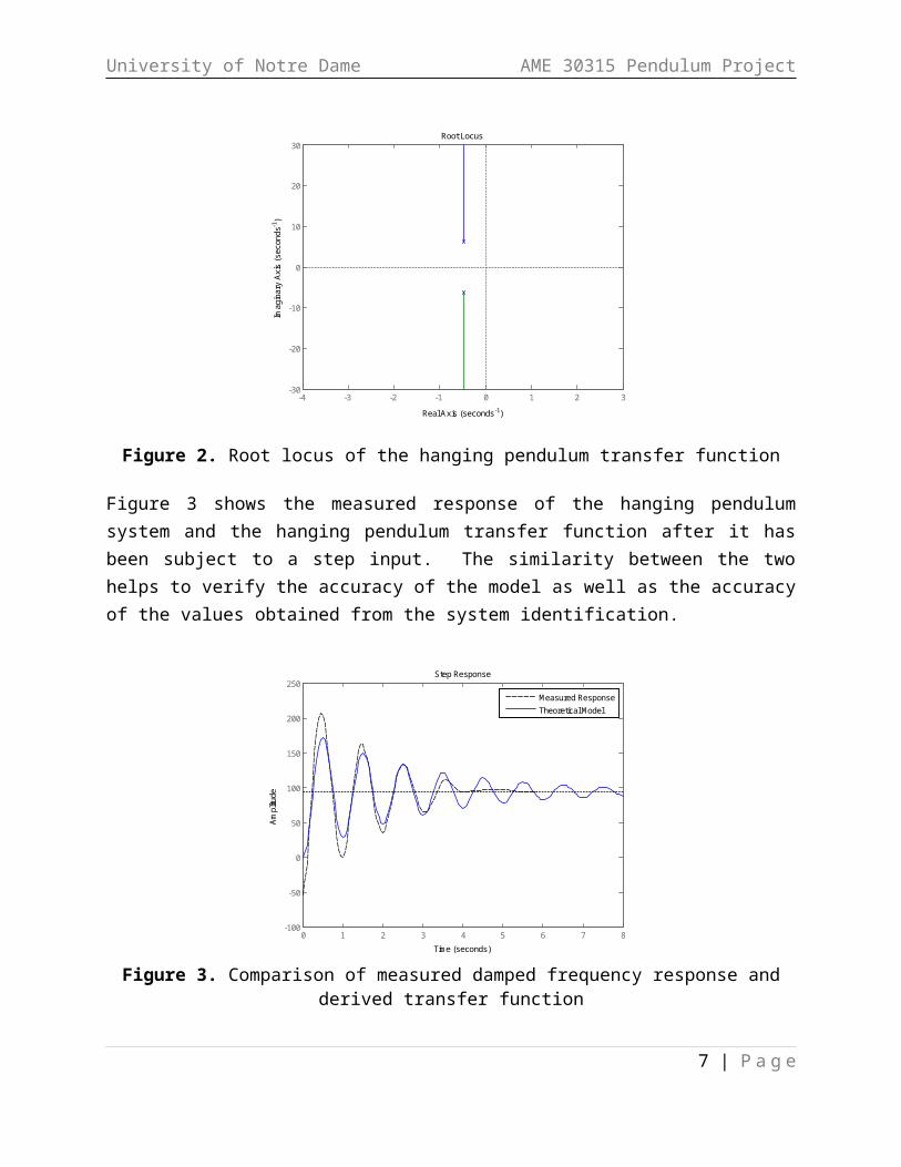
Figure 3 is the root locus of the invert pendulum transfer function.

7 | P a g e


-8 -6 -4 -2 0 2 4 6 8-8

-6

-4

-2

0

2

4

6

8Root Locus


Imag

inar

y Ax

is (s

econ

ds-1

)

Figure 3. Root locus of the inverted pendulum transfer function

Of interest to us at this point is the location of the poles because these will help to determine many of the characteristics of our lead and lag controllers. These poles are at 5.93 and -6.62.

2.2 Design ParametersThe design of the controller is dictated mostly by the desired response characteristics. Therefore before we can begin to design the controller, it is useful to specify a few parameters. The parameters are:

(1)Rise time of 0.5 seconds or less(2)Damping ratio of 0.32(3)Lag gain of 92

These parameters will be used as a guide to the design of a lead and lag compensator.

2.3 Lead Control Lead compensator is a fairly easy and effective means to approximate Proportional-Derivative, PD, control. The idea behind PD control is that the control system should reflect the derivative of the error of the system. Quite simply how large the control input should be should depend upon whether the error is increasing or decreasing. The lead compensator provides phase lead. This shifts the poles to the left, which enhances the stability and performance of the system.

8 | P a g e


2.3.1 DesignThe lead compensator is of the form

Gc (s)=s+zs+p (6)

where z is the location of the lead zero and p is the location of the lead pole.

The angle to the compensator pole must be

∠G (s )=θz−θ p1−θp2−θ p3=−180 ° (7)

because points on the root locus satisfy ∠G (s )=−180 °, we can use the angles from the two poles and one zero to the desired point to compute what the angle from the compensator pole must be.

2.3.2 Lead CalculationCalculations for the lead controller are done using the Matlab function pole_loca shown in Appendix E. This function takes the location of the transfer function poles as well as a desired zero and outputs a minimum lead pole location. A large part of the lead design is dictated by the assigned damping ratio value. This is because,

ξ=sin θ (8)

where θ is given by the root locus plot. A small amount of control over the lead design is exercised in the placement of the lead zero. This zero was placed as close as possible to the plant pole in order to mitigate any adverse effects the zero would have on the response of the system. Using a zero at -7 a pole of -8.5 is needed to meet the minimum design specifications. The gain needed to obtain the correct damping ratio was then k=221. However this design did not seem optimal. To optimize the design it was decided that the lead pole needed to be moved farther left in order to increase its effect on the root locus. The actual placement of the pole was found through an iterative process. This process and comments on response can be found in Appendix F. The final design of the lead compensator is shown in Equation 9.

s+7s+17.5 (9)

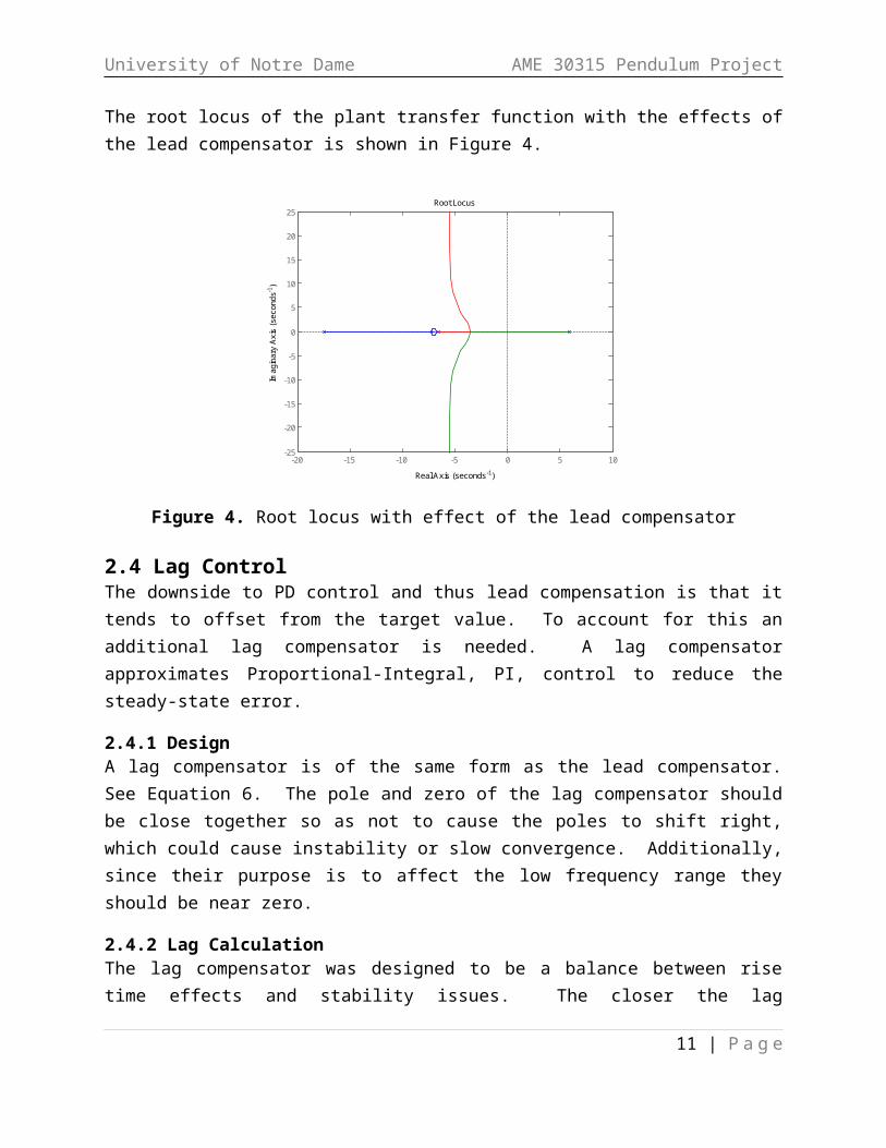
The root locus of the plant transfer function with the effects of the lead compensator is shown in Figure 4.

9 | P a g e


-20 -15 -10 -5 0 5 10-25

-20

-15

-10

-5

0

5

10

15

20

25Root Locus


Imag

inar

y Ax

is (s

econ

ds-1

)

Figure 4. Root locus with effect of the lead compensator

2.4 Lag ControlThe downside to PD control and thus lead compensation is that it tends to offset from the target value. To account for this an additional lag compensator is needed. A lag compensator approximates Proportional-Integral, PI, control to reduce the steady-state error.

2.4.1 DesignA lag compensator is of the same form as the lead compensator. See Equation 6. The pole and zero of the lag compensator should be close together so as not to cause the poles to shift right, which could cause instability or slow convergence. Additionally, since their purpose is to affect the low frequency range they should be near zero.

2.4.2 Lag CalculationThe lag compensator was designed to be a balance between rise time effects and stability issues. The closer the lag compensator values were to zero the less effect they had on stability. However, if these values were too close to zero, they negatively affected rise time. The placement of the lag zero, and thus the lag pole, was also determined through an iterative process. A lag zero was chosen and then a lag pole was calculated using the lag gain ratio. The final design of the lag compensator is shown in Equation 10.

10 | P a g e

FirasFasheh, 05/04/12,

Defining was PI and PD are might be a good idea


s+1.2

s+1.292

(10)

The root locus of the transfer function with the lead-lag compensator is show in Figure 5. The point shown corresponds to the optimal gain value used.

Root Locus


Imag

inar

y Ax

is (s

econ

ds-1

)

-20 -15 -10 -5 0 5 10-30

-20

-10

0

10

20

30System: sysGain: 7.01Pole: -4.22 + 10.7iDamping: 0.366Overshoot (%): 29.1Frequency (rad/s): 11.5

Figure 5. Root locus of the transfer function with the lead-lag compensator

2.5 Discrete-time Transfer FunctionUp to this point the entire controller design has been in continuous-time. However, the microcontroller only works in discrete-time. Therefore the controller must be converted from continuous-time to discrete-time.

2.5.1 Conversion to Discrete-timeThe Tustin method allows us to switch from continuous time to discrete time by substituting in the following equation for s,

s= 2T

1−z−1

1+z−1 (7)

where T is the integration step size. The Matlab c2d command can be used to make this substitution. For completeness hand substitutions for a single lead-lag controller were also done. Appendix C shows these substitutions.

3 Controller Implementation

11 | P a g e


3.1 Controller ImplementationThe controller is implemented in discrete-time using the substitution described above. Additional steps are described below.

3.1.1 Non-dimensionalizationAll terms relevant to the control system are non-dimensionalized. This was done for two reasons. (1) It allows for units to be taken in to account at the end of the program and (2) It allows for easier debugging because all important parameters have to be between 0 and 1. Because we had no real sense of what sorts of values we should expect from the torque at various positions, it is much easier to catch an error this way.

3.1.2 Error CalculationThe error is calculated by subtracting the current position from the desired position and then multiplying by a scale factor which includes the gain. This value is then divided by the approximate maximum position which non-dimensionalized the error.

R=k ( posdesired−pos )( 1000posmax ) (8)

where R is the error in the current system, and k is the gain.

3.1.3 Transfer Function ImplementationThe transfer function is implemented by solving for the output value, the torque. This torque is a function of the current error in the system, the previous loop’s error value, the error two loops previous, the previous loop’s torque, and the torque two loops previous all scaled by coefficients obtained from the discrete transfer function. For example the implemented transfer function looked something like this,

T=aR+b Rprev+c Rprev 2+d T prev+eT prev 2 (9)

where a ,b , c , d , and e are the coefficients obtained from the discrete transfer function, R is the error in the system, T is the output torque and prev and prev2 denote the previous and twice previous values, respectively. Additionally, a code needed to be implemented that kept the applied torque between -400 and 400. This restriction was caused by supplied PWM.

5 System EvaluationWhen the program was run the following errors were displayed:

“filename.c: In function `main':

12 | P a g e


filename.c:65: warning: unused variable `i'C:\usr\bin\..\lib\gcc-lib\m6811-elf\3.3.6-m68hc1x-20060122\..\..\..\..\m6811elf\bin\ld.exe:ldscripts/m68hc11elfb.xbn:264: warning: memory region eeprom not declared”

The first warning, “unused variable” comes from a counter that was occasionally used to stall the program while evaluating system performance. Neither warning affects the programming of the controller.

5.1 Theoretical ModelingA theoretical model of the controller was implemented using the Simulink block diagram shown in Figure 4.

Figure 6. Representative Simulink block diagram

The response of the system is compared against the results presented in Simulink to get a more thorough understanding of system performance. Figure 7 shows the response predicted by Simulink.

13 | P a g e


Figure 7. Response predicted by Simulink

5.2 Transient EvaluationThe transient response was evaluated by looking at the rise time and the overshoot. Figure 8 shows the response of the pendulum.

0 2 4 6 8 10 12 14-300

-200

-100

0

100

200

300

time [s]

disp

lace

men

t [en

code

r cou

nts]

Figure 8. Response of pendulum

5.2.1 Rise Time EvaluationSimulink predicts about a 0.2 s rise time. The pendulum itself has a rise time of approximately 0.6 s. Although these values differ, the pendulum almost perfectly meets the designed for rise time of 0.5 s. This difference in rise time is mostly likely attributed to neglected values in the derivation of the transfer function. Slipping of the pendulum arm at the point of contact of the motor is not considered. The elasticity of the pendulum is also not considered. Both of these factors could contribute to a longer rise time.

5.2.2 Overshoot EvaluationSimulink predicts an overshoot of about 45%. The actual pendulum, however, has an overshoot of nearly 150%. Part of this error can be attributed to the fact that the microcontroller can only take values for torque within the 400/-400 range. The overshoot could be further exasperated by the fact that the microcontroller only takes integer values for input torque. A more precise system that takes decimal inputs could decrease this error. The errors are compounded by the discretized controller system. The torque is computed by using the previous two error

14 | P a g e


and torque values. If these values are themselves in error then the torque could overcompensate and therefore increase the overshoot value.

5.3 Steady-State EvaluationTo evaluate the steady-state response of the system a program is run and swept through a variety of angles. The approximate errors at these angles are tabulated in Table 1. This table shows that as the displacement increases, the error increases. This result is most likely due to the small angle approximation made during the derivation of the transfer function. Additionally, the error seems greatest when the desired value is negative. This error is most likely caused because of the way the motor applies the torque. More than likely the motor has a certain direction that it prefers to apply a torque. This direction would have a stronger and more constant value than the ‘reverse’ direction. This is probably what is causing the greater error on the negative displacement side.

Table 1. Steady-state error in the controller at various desired angles.

Desired Angle [°]

Error [°]

Desired Angle [°]

Error [°]

-30 -1.5 0 1-20 -1.5 10 0.5-10 -1 20 00 1 30 1

Figure 9 shows the response of the system as it is being swept through the various angles. It’s interesting to note that although there is a small amount of steady-state error associated with the system, the rise times and overshoots stayed relatively constant. Additionally, the settling time of the system can be computed from Figure 9. Simulink predicts a settling time of about 6 s. The actual pendulum settles in about 4 s. This lowering of the settling time of the actual pendulum could be attributed to the increase in overshoot, by overshooting so much the controller requests additional torque from the motor. This additional torque acts to quickly forces the pendulum to its steady-state value.

15 | P a g e


0 5 10 15 20 25 30 35 40 45 50-300

-200

-100

0

100

200

300

400

time [s]

disp

lace

men

t [en

code

r cou

nts]

Figure 9. Response of pendulum at angles of -30º to 30º

6 System Verification6.1 Position VerificationTwo videos were taken of the pendulum. The first simply tests how the pendulum responds to being displaced. The second video is used to verify the pendulum at a variety of different positions.

A video of the pendulum in operation can be found at the following link:

http://www.youtube.com/watch?v=Z4SMefuY2cM&feature=youtu.be

A video of the pendulum operating at a variety of different angles can be found at:

http://www.youtube.com/watch?v=E_No3QtmH2g&feature=youtu.be

7 ConclusionsIn conclusion, the controller worked for the values assigned in the project document. However it is found that by increasing the gain and moving the lead pole farther left, increased a smaller overshoot could be attained. The theoretical model of the pendulum did a very good job of predicting rise time and settling time. However the Simulink model way under predicted the amount of overshoot experienced by the system. This difference in overshoot can be explained in the way that the microcontroller inputs torque as well as assumptions made in the creation of the transfer function. To improve the accuracy of the controller, a few things could be done. A

16 | P a g e

http://www.youtube.com/watch?v=E_No3QtmH2g&feature=youtu.be

http://www.youtube.com/watch?v=Z4SMefuY2cM&feature=youtu.be


different microcontroller could be used that accepts decimal inputs. Additionally, the efficiency of the evaluation of the system could be increased by purchasing a microcontroller that uploads significantly faster. A majority of the analysis time for the pendulum was spent waiting for the program to upload.

17 | P a g e


Appendix A

18 | P a g e


19 | P a g e


Appendix B/* Basic code skeleton for AME 30315 Project Inverted Pendulum

---------------------Real Code---------------------- Authors: Bill Goodwine, April 6, 2009. Raymond Le Grand, May 26, 2010. Blair Rasmus, Derek Wolf, John Gallagher, November 13, 2011*/ #include "hc11.h"#include "mc.h"#include <math.h>#include "vectors.c"#include "serial.c"

// the next two lines setup constants for direction of pendulum#define CW 0#define CCW 1 #define OFFSET 1777//This is the difference between the encoder zero and the pendulum straight up position.//This may change slightly with each pendulum.

#define SCALE 18 /* the SCAlE constant represents the scale of the position decoder, which is degrees per signal tick, but since the microcontroller only does integer math,we will define the scale as an integer and divide by 100 every time.*/

#define MAX_U 400 /* The MAX_U constant represents the maximum amount of PWM signal that the system can handle,without the signal being so fast that there are current/voltage spikes.It is strongly recommended that this value not be changed.*/#define CONTROL_LOOP_FREQ 20 //Frequency of control loop calculations in Hz#define CLOCK_FREQ 9830400#define PWM_FREQ 880

// Initializing controller variableslong pos=0, R=0, R_prev=0, R_prev2=0, T_prev=0, T_prev2=0;//int pos_deg=0; //keeps track of current angle. 'pos' is in encoder counts, and 'pos_deg' is in degrees*100

// Initializing PWM variablesunsigned int counts_total=((long)CLOCK_FREQ/4)/PWM_FREQ;// counts_total is used for the counter for the PWM interrupt. This should give a 880Hz interrupt. // We divide the clock frequency by 4 because the counter increments every fourth clock cycle when using a prescale of 1unsigned int counts_high;

20 | P a g e


unsigned int counts_low;

// Initializing Timing Variablesunsigned int PWM_interrupt_scale=PWM_FREQ/CONTROL_LOOP_FREQ; //Sets the ratio of PWM interrupts to control loop interruptsunsigned int PWM_interrupt_counter = 0; //this keeps track of ticks from control loop interrupt, used for timing

// My variablesunsigned int time=0;long k=6;long posD=0;

int main(void){

//Initializing controller variableslong u=0; //This is what we use to store the calculated value for torque that we needint i;// Initialize hardwareinit_ports();init_interrupts(); //this also init's the interrupts for tracking positionset_torque(0); //starts out at 0% torque pause(brief); // power-on delayinit_serial(); //Initialize serial communication welcome(); //Display welcome messagepause(brief);set_zero();//Example of how to write to serial port//out_string("Here is an example of a printed number: ");//out_string("-");//out_unsigned_dec(24);while(1){ //this checks to see if the pendulum is in top position, //which allows for greater position accuracyif(check_encoder_top()){pos = OFFSET/18; //pendulum has reached center, so reset position to zero + OFFSET.}PORTA ^= 0x10; //0b01000000; //toggle pinA.4 on/off to show user that interrupt is 20Hz with blinking LEDif(PWM_interrupt_counter>=PWM_interrupt_scale/*control_loop_limit*/){ //this checks to see if it is time to do 20Hz control calculationsPWM_interrupt_counter=0;PORTA ^= 0x40; //0b01000000; //toggle pinA.6 on/off to show user that interrupt is 20Hz with blinking LED//////////////////////// 20 Hz Operations///////////////////////////////////////This where you need to calculate/set the torque//////////////////////pos_deg=pos*((int)SCALE); //calculate the current position in degrees*100

// Print position to find damping out_unsigned_dec(time); out_string(" ");

21 | P a g e


if(pos<0) {out_string("-");out_unsigned_dec(-pos);}else {out_unsigned_dec(pos);}carriage_return();

R = (posD-pos)*(1000/378)*k;// R = non-dimensionalized error in the current position

u = (8416*R -13840*R_prev + 5565*R_prev2 +13910*T_prev -3910*T_prev2)/10000;// T = non-dimensionalized torque

//u = 400; if(u>1000) { u = 1000; } if(u<-1000) { u = -1000; }//set_torque(250);set_torque(-u*400/1000);

R_prev2 = R_prev;R_prev = R;

T_prev2 = T_prev;T_prev = u;

// for (i=0;i<10;i++){// pause(SECOND);// }// set_torque(-u);// for (i=0;i<10;i++){// pause(SECOND);// }///////////////End of 20Hz Operations////////////////////////////////////////time = time+50;if(time==7000) {posD = -173;}if(time==14000) {posD = -117;}if(time==21000) {posD = -61;}if(time==28000) {posD = 0;}if(time==35000) {posD = 53;

22 | P a g e


}if(time==42000) {posD = 104;}if(time==49000) {posD = 160;}}}}

/**** This begins the Interrupt Code ****/

// Programing interupts for PWM void OC3_handler(void){ if(!(PORTA & OC3)){ //(portA.5==low) so set the TOC3 to the time at which we want to end the low part of the PWM cycleTOC3 = TOC3 + counts_low;}else{TOC3 = TOC3 + counts_high; // Set TOC3 to the time at which we want to end the high part of the cyclePWM_interrupt_counter++;} TFLG1 |= OC3; }

// Programming Interrupts for Tracking Movementvoid PAI_handler(void){//this checks direction of pendulum, then increments position variableif((PORTA & 0x02 /*0b00000010*/) == 0){pos++;}else{pos--;}TFLG2 |= PAIF; //reset interrupt flag}

/* default interrupt handler (empty, just returns) */void default_handler(void) {}

/**** End of Interrupt Code ****/

// Function to initialize PWMvoid init_interrupts(void){// this also initializes position encoder

asm(" sei"); //disable interrupts BAUD=BAUD9K_Turbo; //Use BAUD38K for non-turbo mode of microcontroller

// set register to next time for each interrupt TOC3 = TCNT + counts_total; // arm all interruptsTMSK1 = 0x0; TMSK1 |= OC3;

23 | P a g e


//pulse accumulator setup: used to receive signal from decoder that gives pendulum angleTMSK2 |= 0x10; //0b00010000; this enables pulse accumulator interrupt

// acknowldege all interrupts, in case they were already triggeredTFLG1 |= OC3; //flag for pulse accumulator TFLG2 |= PAIF; //flag for pulse accumulatorPORTA |= (OC3); //start off both PWM ports highTCTL1=OL3; /*want PORTA.5 to toggle every time there's an interrupt, but nothing else*/

TCTL2=0xC0; //0b11000000; // this turns on error checking from h-bridge on pinA3 asm(" cli"); //enable interrupts}

// Function to set PWM duty cycle, which changes torquevoid set_torque(long p_rate){// Accepts desired Torque percentage as an input, and uses the global direction flag to know which direction to apply torque

while((PORTA & OC3)); //while (portA.5==high) do nothing, //b/c want to wait until low cycle has started, //which means that we can load next high-low cycle without messing up PWM period

// This calculation is 50% + (p_rate%).// 50% PWM = 0torque, and 95% PWM is Max torque in CW direction.p_rate=((unsigned int)(counts_total/10)*p_rate)/(unsigned int)10;counts_low=(unsigned int)counts_total/(unsigned int)2-p_rate/(unsigned int)10; //divide p_rate by ten to get it as 0-40 instead of 0-400

counts_high = counts_total-counts_low;}

// Read direction signalunsigned char check_encoder_dir(void){unsigned char dir_flag;if((PORTA & 0x02/*0b00000010*/) == 0){dir_flag=0;}else{ dir_flag=1;}return(dir_flag);}

// Read vertical position sensor (tells when pendulum is vertical)int check_encoder_top(void){int top_flag;

//this checks pin A.2 to see if pendulum is verticalif(!(PORTA & 0x04/*0b00000100*/)){ //note that this line was inverted to account for top signal being invertedtop_flag=0;}

24 | P a g e


else{top_flag=1;}return top_flag;}

// Pause function waits for specified number of clock cycles before continuingvoid pause(unsigned int duration){unsigned int time;time=duration; // small delay routinewhile(time>0)time--;}

// Initialize portsvoid init_ports(void){/* enable pulse accumulator on PA7, falling edgePA3 is input capture IC4 */ PACTL = 0x40; //0b01000100; //PACTL = 0b00000100; //this is the code to disable itPORTA = 0xCF; //0b11001111; // disable H-bridge, photointerrupterDDRD = 0x07; //0b00000111; // sets D0-D2 as outputs, the rest are inputsPORTD = 0x04; //0b00000010; // clears Port DPACNT = 0x00; //0b00000000; // clear Pulse Accumulator }

// Function to prompt user to move pendulum through zero to initialize angle countervoid set_zero(void){ int de_ch=0,index=0; while((PORTD & 0x08 /*0b00001000*/) == 0); // make sure ok button has been released out_string("Move Through Vertical Position"); carriage_return(); pause(SECOND); pause(SECOND); pos=0; out_string("DIR POS "); carriage_return(); while(check_encoder_top()==0){ //checks to see if pendulum is at top position

//if pendulum not at the top, then keep looping

de_ch=check_encoder_dir(); //check the direction of the pendulumif(index==1000){ // only updates screen every 1000 iterationsout_unsigned_dec(de_ch); //print out direction

25 | P a g e


//output position, account for positive/negative numbersif(pos>=0){out_string(" ");out_unsigned_dec(pos*SCALE/100);}else{ out_string("-"); out_unsigned_dec(-pos*SCALE/100);}out_char(NEWLINE); //go back to column zero, but same lineindex=0;}else{index++;}}//pendulum has reached the top,so stop loopingpos = OFFSET/18;carriage_return();out_string("you finished!");carriage_return();pause(SECOND);}

// Displays Welcome messagevoid welcome(){pause(brief);out_string("AME 30315");out_string(" Pendulum Project ");carriage_return();carriage_return();}

// initialize MicroStamp 11. This function is called by _start, which is defined in crs0.s// A __premain() is created by default by GCC compiler, but we have overwritten the default // so that we can move the register block, which must be done within first 64 bus cycles void __premain(void) {*(unsigned char volatile *)(0x3D) = 0x01; //Register block will start at 0x1000 instead of default 0x0000TMSK2 = 0x0C; //0x0D; // =1101b, a prescale of 4 for the output compare, // which must be set within 64 cycles of microcontroller reset,// which is why we set it hereCONFIG = 0x04; // disable COP timer}

26 | P a g e

pendulum project - university of notre damejszczud1/pendulum project report.docx · web...

Documents