peer-reviewed article bioresources · sbarbaro et al. 2002; paiva et al. 2004; rajesh and ray 2006;...

PEER-REVIEWED ARTICLE bioresources.com

Zhang et al. (2016). “Brightness control model,” BioResources 11(2), 3660-3678. 3660

Improved Model for Brightness Optimization Control in the First (C95/D5) Bleaching Stage

Xiangyu Zhang, Jigeng Li,* and Huanbin Liu

In the first stage of pulp bleaching, the quantity of added chemicals (ClO2 and/or Cl2) is commonly controlled by kappa factor, based on a kappa number online analyzer together with a compensated brightness control scheme as a feedback strategy. However, a kappa number analyzer is not always available, so the bleaching quality relies heavily on the chemical dosage set-point chosen by the operators. In this study, an improved model for the chlorination stage brightness optimization was proposed, based on brightness and residual chemicals before pulp enters the bleaching tower. Additionally, the experience of operators of (C95/D5) bleaching was employed in order to find an optimum chemical dosage set-point quickly. The golden section search algorithm (i.e., ‘0.618 method’) was used to find the optimum chemical dosage in this paper. After applying the proposed method in a pulp mill (C95/D5) bleaching stage, the chlorination stage brightness shifted from 62.9% ISO to the target value 60.7% ISO. Meanwhile, the standard deviation was reduced from 3.0 to 2.5.

Keywords: Kraft pulp; Bleaching; Brightness; Optimization model; Variance reduction

Contact information: State Key Laboratory of Pulp and Paper Engineering, South China University of

Technology, Guangzhou 510640, P.R. China; *Corresponding author: [email protected]

INTRODUCTION

The main objective of pulp bleaching is to increase pulp brightness within specified

limits. Chemical agents are applied in sequential stages to achieve the correct brightness

(Flisberg et al. 2009). Bleach sequences vary widely from mill to mill, but the first stage is

commonly the chlorine dioxide delignification (D0) or chlorination (C or (C95D5)) stage;

chlorine is still permitted for bleaching in a few regions in China. In the (C95D5) stage,

unbleached or oxygen-delignified pulp is treated with chlorine (Cl2) and chlorine dioxide

(ClO2) to decrease the kappa number (lignin content). The necessary chemical dosage

depends on the incoming pulp’s lignin content.

Kinetic models of chlorine dioxide (D0), chlorine dioxide substitution ((CD)), and

chlorination (C) have been researched. In the D0 stage, a very fast delignification reaction

occurs, followed by a slow one (Savoie and Tessier 1997). Likewise, the pulp brightness

increases quickly during the first few minutes and then increases more slowly. Ackert et

al. (1975) developed a model for chlorination that divides lignin into three types: fast

lignin, slow lignin, and floor lignin. When the contents of fast, slow, and floor lignin are

each expressed as a kappa number, the initial kappa number is equal to their sum (Ackert

et al. 1975). This concept was later adapted to the D0 stage from the C stage. The model of

the fast and slow lignin removal rates consists of two ordinary differential equations

(Tessier and Savoie 1997; Jain et al. 2009), which can be used to determine the chemical

charge and temperature required for achieving the desired delignification. Though the



reaction consists of two phases, the relationship between chlorine consumption and kappa

number decrease is linear and independent of the incoming pulp kappa number.

Additionally, the pulp brightness has a linear relationship with the kappa number after the

first stage (Tessier and Savoie 2000).

To predict chemical usage, kappa number, brightness, and residuals after the first

bleaching stage, empirical and semi-empirical mathematical models based on experimental

and operating conditions usually have been used for dynamic simulation of the bleaching

process (Wang et al. 1995; Savoie and Tessier 1997; Tessier and Savoie 2002; Gu and

Edwards 2003; Yoon et al. 2004). Statistical methods, polynomial regressions, and

stoichiometric calculations have been employed in the modeling process, and those models

could be used for bleach plant optimizations, computer simulations, and process control

(Brogdon 2012, 2013, 2014). Because of the complexity of the bleaching process and its

nonlinear and time-varying characteristics, models based on identification methods and

neural networks have been shown to be efficient in process control (Perala and Kirby 2001;

Sbarbaro et al. 2002; Paiva et al. 2004; Rajesh and Ray 2006; Flisberg et al. 2009; Ferrer

et al. 2011). In a modern bleaching plant, model-based control strategies provide an

efficient way to achieve better control results where online and inline sensors are widely

applied (Tessier et al. 2000; Mercangöz and Doyle 2006).

In the D0 stage, a feed-forward kappa factor control with compensated brightness

quick feedback from the brightness and residual sensors provides good results (Tessier et

al. 2000). Unfortunately, not all mills can afford a kappa analyzer and the associated

maintenance costs. Even if a kappa analyzer is available, the kappa factor control may not

follow the variance of kappa number in the sampling period (about 20 min). In this paper,

a model for optimizing the chemical dosage in the (C95/D5) stage is presented. The model

is based on the brightness and residual values provided by online instruments. These two

values were obtained before the pulp entering into the chlorine tower. When the model was

applied, it could reduce the variance of brightness after chlorination stage and shift its

targets.

EXPERIMENTAL

C95/D5 Stage Bleaching Process Description The focus of this paper was the (C95/D5) stage of a eucalypt kraft pulp mill. Its

bleaching sequence was O-(C95/D5)-(EOP)-D; the (C95/D5) bleaching process is

simplified in Fig. 1.

After washing, the oxygen-delignified pulp was conveyed into the brown stock

tower and diluted to a suitable consistency. The control system for the first stage included

local feedback loops for consistency and flow rate control. The stock consistency and flow

rate could be controlled steadily and maintained at a target production rate. The pulp

consistency was 2.8%, and the flow rate was 8.6 m3/min during this process. The diluted

pulp was then pumped into the mixer and mixed with the chemicals ClO2 and Cl2. Their

ratio was 5% to 95%, respectively, and the ClO2 solution had a concentration of 7.4 g/L.

The mixed pulp was continually pumped into the (C95/D5) bleaching tower, which was an

up-flow tower. The length of time that the pulp stayed in the tower depended on the

production rate, but was generally approximately 30 min. The bleaching reaction started

when the pulp mixed with the chemicals and was nearly completed when the pulp

overflowed from the bleaching tower.



The kappa number Koff-line after the oxygen delignification stage (O stage) was

controlled to a target of 11 to 12 in an ideal situation and tested in a lab every 2 h. However,

the kappa number Koff-line was often in excess of the specified value range and brought

fluctuations of the applied dosage of bleaching chemicals. The residual alkali in pulp (the

percent of residual alkali in 100 gram pulp) after the oxygen delignification stage is a

disturbance for kappa factor control methods in the first bleaching stage. In this bleaching

process, the residual alkali ranged from 0.36% to 0.40% after the oxygen delignification

(O) stage in the pulp washer. The brightness after chlorination stage Boff-line was tested in a

lab every 2 hours, and the desired brightness was 60% ISO, corresponding to the desired

incoming kappa number of 11 to 12. If the initial kappa number was not the desired value,

then controlling the chlorination stage brightness to the target value of 60% ISO is difficult.

The bleaching temperature in the tower was maintained at 56 ºC. The online brightness

analyzer (BI) and residual sensor (RI) were added before pulp entered the bleaching tower.

The sampling time for brightness (b) and residual (r) in the DCS system was every 6 sec.

BI

Brown stock

Tower

Mixer

Dilution

Water

(C95/D5))

Bleach

TowerfD

fP

cP

pD

ClO2

making

plant

Pulp consistency and flow rate control

vp1vp2

vc1 vc2

vD

RI

belt conveyor

Ttower

Cl2

Tank

vC

I-1

fC

I-2

pC

Fig. 1. Schematic diagram of the (C95/D5) bleaching stage

Generalization of a Human-supervised, DCS-based Process The purpose of the bleaching stage (C95/D5) is to decrease the kappa number. The

variation of kappa number is the main disturbance in the (C95/D5) stage. If the kappa

number analyzer is available, the kappa number together with online brightness and

residual provided both feed forward and feedback measurements for improved control

(Tessier et al. 2000). If not, the compensated brightness control method was beneficial all

by itself. As early as 1975, a control strategy based on a dual oxidation reduction potential

ORP probes (one was mounted on before brown stock entering into bleach tower and

another was on the outlet line after bleach tower) was applied in a bleach plant (Danforth



et al. 1975). The sensor after the tower gives information on how well the chlorination

stage is functioning, but due to the long delay, it is not adequate for feedback control.

Afterwards, sensors are also located between the mixer and the tower or at the bottom of

the tower (Rankin and Bialkowski 1984; Corbi et al. 1986; Dumont et al. 1989).

Generally, when the ORP sensors were applied in the chlorination stage, the control

strategies was the chlorine flow which was adjusted by a PID controller for regulating the

pre-tower ORP sensors value (Cl2 residual) to the input residual set point. The second ORP

probe was used to measure the chlorine residual for feedback control and to provide

information needed to adjust the pre-tower residual set point. The residual set point could

be adjusted as a function of the unbleached pulp kappa number. However, if kappa number

is not obtained easily, it would usually be adjusted by operators based on their experience

(Danforth et al. 1975; Dumont et al. 1989; Diaz et al. 1992).

Because an optical sensor could be applied to measure pulp brightness, a

combination of residual and brightness signals as a weighted sum, what has become known

as the ‘compensated brightness’ signal, and is most commonly adopted in first bleaching

stage. Compensated brightness control regulates the dosage of the chlorine mixture to

achieve target brightness after a one minute reaction time, leaving a residual amount of

chemical to complete the reaction in the bleaching tower. The total applied chemical is

used with a regression model for the calculation (Rankin and Bialkowski 1984; Corbi et al.

1986; Cunningham 1993). The compensated brightness value is often fed to a conventional

PI controller to maintain a constant brightness, which in turns cascades down to either the

chlorine and or the chlorine dioxide flow controller (Van Fleet 1998), as shown in Fig. 2.

Bleach

TowerBI RI

Compensated Brightness=

k1×b+k2×r

Cl2

Set point+

-

Brown Stock

Compensated

Arithmetic

ClO2

Ratio

Fig. 2. Flow sheet for compensated brightness control

The essential aspect of the compensated brightness control is how to adjust the

target brightness set point, which could be determined by pulp brightness after tower and/or

reset by a feed-forward model for predicting incoming brown stock kappa number (Rankin

and Bialkowski 1984; Corbi et al. 1986; Cunningham 1993). Typically, the set point has

been determined from the operators’ comprehensive on the process behavior (Lampela et

al. 1996).

In the (C95/D5) stage, in order to compensate for incoming kappa number swings

and other possible disturbances, besides the compensated brightness control strategy,

operators often have been required to determine the proper set-point values in terms of

ClO2 flow, Cl2 flow, and sometimes pulp flow to maintain satisfactory performance, based

on various experiments and their own expertise, as shown in Fig. 3.

The supervisory control process can be described as follows: when the incoming



kappa number is changed, the disturbance ΔK causes a variation of brightness (b) and

residual (r). The two values b and r were measured by Metso Kajaani CORMECS

brightness analyzer and Kajaani POLAROXS chemical concentration measurement sensor

(Metso Automation Inc., Finland), respectively. The operators can determine the deviation

of b and r from the optimum values corresponding to current process conditions. Then,

they are able to regulate the chemical flow set-point to meet the changed process conditions,

according to their experience.

Decision

Making

Operator

Experience

DCS(C95/D5)

Bleaching

Stage

rbBoff-line

ΔrΔbΔBoff-line

RI

Brightness

Lab Test

Koff-linePulp Flow

Cl2 Flow

ClO2 Flow

ΔK

BI

Fig. 3. Human-supervised, DCS-controlled (C95/D5) bleaching process

The operators were able to evaluate the previous regulated lab-tested values Koff-line

and Boff-line, which also played an important role in enhancing their skills and experience,

increasing operator confidence of maintaining satisfactory performance.

Either compensated brightness alone or along with human supervision, the core

way to regulate the applied chemicals is based on the assumption that a lower pre-tower

brightness with a higher residual will eventually react with the pulp to produce a higher

brightness after being discharged from the tower. Ultimately, the optimum process

condition is one in which off-quality pulp is not produced and chemical is not over-applied.

Definition of Optimum Process Conditions In (C95/D5) bleaching stage, the kinetics of chlorine bleaching with low chlorine

dioxide substitution are assumed to be the same as with chlorine bleaching (Wang et al.

1995). Ackert et al. (1975) proposed a kinetic model of lignin reaction with Cl2. It was

assumed that the two first-order reactions are taking place in parallel and was described by

the following equations (Eqs. l through 4), where KC,f and KC,s denote the content of fast-

and slow-reacting lignin expressed as a kappa number, [Cl2] denotes the concentration of

chlorine (mol/L), and RC,f and RC,s denote the rates of the fast and slow lignin removal,

,

, , 2 ,

C f

C f C f C f

d KR k C l K

d t (1)

,

, , 2 ,

C s

C s C s C s

d KR k C l K

d t

(2)

where the reaction rate constants kC,f and kC,s are expressed as (Wang et al. 1995):



,

2 5 01,1 2 3 ex p ( )

C fk

T

(3)

,

2 5 02 2 .4 7 ex p ( )

C sk

T (4)

It was obvious that the rate of the fast lignin removal was much faster than that of

the slow lignin, according to kC,f and kC,s, where kC,f was more than 50 times higher than

kC,s. The fast lignin reaction could be completed in 1 to 2 min. As all of the fast lignin and

slow lignin would have been removed, the delignification reaction was completed in the

first bleaching stage. The remaining unreactive lignin was linked to what is known as floor

lignin.

The kappa number KC is a summation of KC,f , KC,s, and KC,∞ associated with the

contents of fast, slow, and floor lignin, where KC,∞ is the content of floor lignin. The initial

values of KC,f, KC,s, and KC,∞ are in proportion to the initial kappa number KC,0. The

proportionality coefficients were α, β, and γ, and their relationship and values were given

as following equations (Eq. 5 and 6).

0 0, 0 , , , , 0 , 0 , 0

= + +C C f C s C C C C

K K K K K K K

(5)

0 .5 0 .3 0 .2 (6)

In the (C95/D5) stage, the brightness and residual sensors were placed as far after

the chemical injection point as possible, before the entrance of the tower. The flow rate

was usually constant, so that the movement from the chemicals and pulp mixer to the

instrument location took a certain amount of time (about two minutes in the studied

process). It could be deduced that the fast lignin reaction was completed in a few seconds

when the chemicals were mixed with pulp and that most of the slow lignin reaction had

also been completed before entering the tower. Therefore, when a certain quantity of

chemical agents controlled by kappa factor was added to the incoming pulp at a given

kappa number, there were corresponding brightness and residual values. Those two values

varied with the incoming kappa number.

To ensure that the slow lignin was removed and to avoid brightness reversion

(Tessier and Savoie 2002), the residual value should be kept in proportion to the content

of remaining slow lignin (Eq. 7),

**

0=

sr K K

(7)

where Ks* is the content of the remaining slow lignin expressed as the kappa number.

As described in the Kubelka-Munk equation, the pulp brightness is dependent on

the amount of chromophoric groups in the pulp (Brogdon 2014). Lignin is the major

contributor to chromophores (Tessier and Savoie 2002). The brightness before the pulp

enters the tower and can display the extent of the decrease in kappa number and could also

be considered an indicator of the content of unreacted slow lignin and unreactive floor

lignin (Eq. 8).

* *

s 0 0

1 1

( )b

K K K K

(8)



In this case, without considering temperature and final pH (because there was Cl2

in the reaction and pH could be controlled to the desired value), the brightness b and

residual r, together with the amount of total equivalent chlorine per ton of air-dried pulp

provided information about the incoming kappa number, the unreactive floor lignin, and

the remaining portion of slow lignin.

Field data pre-process and analysis

The primary objective for the first bleaching stage is delignification, which is

achieved through oxidation of lignin in the pulp. The subsequent alkaline extraction stage

(second stage) continues to remove the chlorinated organics produced in the first stage after

second stage washer, where a CEK number (the kappa number after the (EOP) stage) was

tested for estimating delignification in the first stage. The control strategy used for the close

association two stages was to adjust the total equivalent chlorine set point to maintain a

constant CEK number.

Based on the target, the evaluation of the first stage control performance is whether

the brightness after chlorination stage (Boff-line) and CEK number were all in the specified

limits. If Boff-line and CEK were good value, the corresponding total equivalent chlorine Q

was taken as the optimum value (Q-bar) to the unbleached pulp kappa number (K).

In the (C95/D5) stage, the sampling locations were the inlet before the mixer and

the outlet of the up-flow chlorination tower. These locations were used to test the pulp

properties of kappa number (Koff-line) and post-tower chlorination brightness (Boff-line). After

the (EOP) stage, a CEK number was also tested.

There was a time lag when pulp flowed in the pipeline and chlorination tower. It is

very important to track changes in pulp properties, and the pulp tracking method proposed

by Rankin and Bialkowski (1984) was employed in this study. After coordinating the

values for Koff-line and Boff-line with the online sensor values, human-supervised control data

over a two-month period were collected from a database in the DCS system. To eliminate

the noise peak jump, lower amplitude, and higher frequency noise, a digital filtering

technique was employed to preprocess the original data.

In daily reports filed by operators there were 12 Koff-line values, 12 Boff-line values,

and 12 CEK numbers tested in a lab every day. Control performance was evaluated based

on CEK and Boff-line data. If their values all were in the specified limits, they would be

chosen as the baseline to look up their corresponding pulp flow, consistency, chemical

addition quantity, and online sensor values (brightness and residual). The found

homologous data was considered as a set of optimum data.

The two months of addressed data were taken as the optimum data group. The data

of each group were composed of Koff-line, optimum quantity of total equivalent chlorine per

ton air-dried pulp (Q-bar), the corresponding online brightness (b-bar), and online residual

(r-bar). All the data were generated at the normal production conditions (including

production rate, pulp consistency, and chlorination temperature and residence time) which

have been given in the C95/D5 Stage Bleaching Process Description in EXPERIMENTAL.

After having been classified and statistically analyzed, the data are summarized in Table 1.

To illustrate the relationship between different kappa number and optimum quantity of total

equivalent chlorine per ton air-dried pulp (Q-bar), the corresponding online brightness (b-

bar), the group data were plotted in a scatter diagram, which suggested there were almost

linearly relationships between Q-bar (Q̅) and b-bar (b̅) with K. Besides, one online



brightness come pair with one residual, and the relationship of corresponding r-bar (r̅) with

b-bar (b̅) was also approximately linear, as shown in Fig. 4.

Table 1. Kappa Number and Corresponding Optimum Process Variables Values

Koff-line 7.8 8.6 9.5 10.2 11.0 12.3 13.4 14.3 15.3

Q-bar (kg/ton a.d.p)

15.2 16.5 17.3 18.7 20.6 23.5 25.1 27.9 30.3

b-bar (%ISO)

59.1 58.3 57.6 56.3 55.0 54.6 53.0 51.8 50.0

r-bar (mg/l)

8.5 9.3 14.6 18.6 22.7 29.5 35.2 38.6 47.9

Boff-line

(%ISO) 62.3 62.0 61.5 61.0 60.2 59.8 58.7 58.1 57.2

CEK number 0.8 0.8 0.9 1.0 1.1 1.1 1.2 1.3 1.3

Fig. 4. The relationship of Q-bar and b-bar with unbleached pulp kappa number (left); relationship of r-bar with b-bar (right)

Optimum process conditions

When diluted pulp with different incoming kappa numbers (K) was mixed with

bleaching agents (Q = the quantity of total equivalent chlorine per ton of air-dried pulp),

there were different corresponding online brightness (b) and residual (r) values before the

pulp entered the bleaching tower, b and r values arise in pairs.

1

2

( , )

( , )

b G K Q

r G K Q

(9)

In equation set (9), the functions G1 and G2 were the real bleach process when

chemical mixed with pulp in the mixer. The quantity of chemical was Q and the kappa

number of incoming pulp was K.

48

50

52

54

56

58

60

0

5

10

15

20

25

30

35

7 12 17

Kappa number

Q-bar

b-bar

48

50

52

54

56

58

60

0 20 40 60

r-bar

b-bar



Kappa number drop is linearly related to the chemical consumption (Savoie and

Tessier 1997), and it is the main indicator of the bleaching load or chemical demand (Van

Fleet 1998). Based on Fig. 4, it can be deduced that the optimum quantity Q-bar and the

initial kappa number K have a linear correlation.

1 1 1( , ) 0F K Q a K b Q c (10)

The parameters a1, b1, and c1 could be determined by a least square method based

on the data in Table 1.

When the applied quantity of total equivalent chlorine was its optimum value of Q-

bar, the corresponding brightness and residual would be an optimum pair b-bar and r-bar.

1

2

( , )

( , )

b G K Q

r G K Q

(11)

When 1 1

1

1= ( )Q a K c

b was substituted in Eq. 11, the results were:

1

2

( , ( ) )

( , ( ) )

b G K F K

r G K F K

(12)

Equation 12 could be simplified to Eq. 13:

1

2

( )

( )

b H K

r H K

(13)

According to the above analysis, it can be concluded that there was a one-to-one

correspondence between the optimum pair (b-bar and r-bar) and the kappa number of

incoming pulp because there was only one optimum Q-bar for the given kappa number

pulp. The pairs continuously varied over different incoming kappa numbers.

1b

K

r K

(14)

Further, there was a correlation between b-bar and r-bar, which can be reasoned

out from Eq. 14. The relationship between b-bar and r-bar was approximately liner as

shown in Fig. 4.

2 2 2( , ) 0f b r a b b r c (15)

The parameters a2, b2, and c2 also could be determined by a least-squares method

based on the data in Table 1.

Therefore, if the online brightness and residual was an optimum pair, their value

would be a solution of Eq. 15. In other words, if b and r was an optimum pair, the current

condition is OPC. Furthermore, a sub-optimal pair accounted for the current Q and was not



an optimum value, and the current process condition was not OPC which would bring about

bleaching off-grade pulp.

Although modern bleaching plants are controlled with the help of inline and online

sensors using advanced control strategies, the operators’ controlling experience is the key

point in optimizing the economic performance and maintaining the bleaching quality. A

model for process optimization was combined ‘compensated brightness’ and expertise

operators’ experience and was developed to improve product quality and reduce the

operators’ burdens.

Model for Process Optimization

The assumption (b,r) was expressed in terms of the online brightness and residual

of the current condition, and X(b,r) was one point of process condition coordinate space

that was made up of brightness and residual before pulp entered the bleaching tower during

the bleaching process, as shown in Fig. 5.

The line ( , ) 0f b r was based on the optimum pairs (b-bar and r-bar) of different

kappa number pulp on the coordinate plane. The control’s job was to regulate the X (b,r)

at optimum condition ( , )X b r .

A line drawn that includes the initial point X (b,r) and intersected the function

( , ) 0f b r at point Or (br,rr). So, f (br,rr) = 0.

Suppose that the slope of this drawn line was k. Then the drawn line could be

expressed as follows (Eq. 16),

( )r r

b b k r r (16)

because of the drawn line intersected with function ( , ) 0f b r , where

2 2

2

1( )k b r c

a .

When the optimal quantity of corresponding chemicals Qr of condition Or (br,rr) was added to the current condition X(b,r), there would be a new process condition

Xr(br*,rr

*).

If f(br*,rr

*) = 0 and br* = br, rr

* = rr, then the pair (br,rr) was regarded as an optimum

one under current process conditions, and Qr was the optimum value.

If f(br*,rr

*) ≠ 0 and br* ≠ br, rr

* ≠ rr, then the pair (br, rr) was not an optimum one

under current process conditions, and Qr was not the optimum value.

In fact, if the process condition Xr(br*,rr

*) fell within the circle with Or(br,rr) as the

center point and ε as the radius, it could be taken as an optimum. If not, regulation is

necessary for an OPC. The ε is a minimum acceptable tolerance to determine whether the

b and r of the process condition could be accepted as optimum values. As shown in Fig. 5,

Drawn Line 1 is an OPC, and Drawn Line 2 is not.

Based on the analysis, an optimization model could be established for reducing the

variance of brightness after chlorination stage and its target could be shifted to a desired

value, which can be applied to brightness control through regulating the quantity of added

chemicals.



Ɛ

X

Or

Or

Xr

Xr

r

b

Ɛ

f (b-bar, r-bar)=0

1

2

Fig. 5. Optimum process conditions in (C95/D5) bleaching process; optimization model regulates the sub-optimal condition into OPC

The distance of a quadratic relationship between Xr(br*,rr

*) and Or(br,rr) can be

treated as an objective function subject to constraints that consist of the process models

and the lower and upper limits of process variables in the (C95/D5) bleaching stage. A

minimization problem was described as follow (Eq. 17),

min * 2 * 2

r r r r( ) ( )z b b r r (17)

where br and rr are obtained from Eq. 18 with Eq. 15 and 16:

2 2 2

0

0

r r

r r

b k r k r b

a b b b c

(18)

To obtain (br*,rr

*), the corresponding optimum quantity chemicals Qr of (br,rr)

should be applied in the bleaching process (Eq. 9).

The relationship of K and b-bar could be deduced from Eq. 13 and Fig. 4. A linear

expression between them was as follow (Eq. 19):

(19)

The parameters a3, b3 and c3 could be determined by a least square method based

on the data in Table 1.

When br was substituted in Eq. 19 together with Eq. 10 as follows, the Qr could be

obtained:

1 1 1

3 3 3

0

0

r

r

a K b Q c

a K b b c

(20)

3 3 3

0a K b b c



After the Qr was applied, br*and rr

* values could be obtained from the brightness

analyzer (BI) and residual sensor (RI). The optimization process is to search a Qr value

until z was less than a minimum value ε2.

The improvement provided by this model is that an appropriate minimum value ε

could ensure a stabilized control performance. There is no regulation when the variations

of b and r are acceptable. Besides, the model could auto-reset the set point of applied

chemicals in response to variations of the unbleached pulp kappa number.

The compensated brightness control strategy is common practice in the pulp mill.

However, the regulation of applied chemicals is often difficult in the optimum case. The

algorithm directly assesses brightness and residual sensor signals combined using

weighting factors, as shown in Fig. 2, and oscillation in the controller’s output are common.

What is more, the major consequence of this strategy is that the operator is forced to over-

apply chemicals in order to ensure that off-quality pulp is not produced (Van Fleet 1998)

through adjusting the target value set point. Thus, the compensated brightness model has

been often unemployable and the DCS control mode is commonly being run on manual

mode, supervised by the operator.

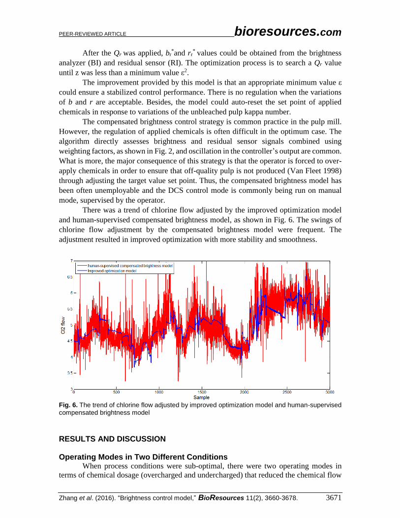
There was a trend of chlorine flow adjusted by the improved optimization model

and human-supervised compensated brightness model, as shown in Fig. 6. The swings of

chlorine flow adjustment by the compensated brightness model were frequent. The

adjustment resulted in improved optimization with more stability and smoothness.

Fig. 6. The trend of chlorine flow adjusted by improved optimization model and human-supervised compensated brightness model

RESULTS AND DISCUSSION

Operating Modes in Two Different Conditions When process conditions were sub-optimal, there were two operating modes in

terms of chemical dosage (overcharged and undercharged) that reduced the chemical flow



or increased the chemical flow. Equation 15 is the relationship between optimum pair b-

bar and r-bar for different initial kappa numbers when the quantity of added chemicals

was optimum. If the process condition was not an optimum one, then b and r were not a

solution to Eq. 15. It was possible to deduce the status of a current condition through the

following rules, where b and r denote the online brightness and residual of the current

process condition:

1) if ( , ) 0f b r ，chemical agent was overcharged;

2) if ( , ) 0f b r ，optimum process condition; or

3) if ( , ) 0f b r ，chemical agent was undercharged

During the bleaching process, the operators’ main job is to quickly adjust or

maintain process conditions at an optimum. If the current process condition is not an

optimum one as shown in Fig. 7, the optimization model could be employed to solve this

problem.

Where Xr(k-1) denotes the current process condition after the last optimized step,

Or(k) denotes the hypothetical optimal condition for the current condition and Xr(k) denotes

the process condition after this time optimization; Or(k+1) and Xr(k+1) denote the next time

optimizing step conditions, if Xr(k) still does not meet requirements.

Ɛ

Xr (k-1)

Or (k)

Or (k+1)

Xr (k)

Xr (k+1)

r

b

Ɛ

f (b-bar, r-bar)=0

Fig. 7. Search procedure for a sub-optimal process condition in the optimization process

Given that the current pre-tower pair brightness and residual was (b1,r2), so the

X(b1,r2) was one point on the coordinate plane of process condition:

1) When b was substituted with 1

b in ( , ) 0f b r , there was a corresponding

value r1; and



2) When r was substituted with 2

r in ( , ) 0f b r , there was a corresponding

value b2

K

K r

bb

Q

r1 r2K1 K2

Q2

Q1

A

(b1,r2)

rK

Q

b1

b2

b

Fig. 8. Operation step of chemicals overcharged in the optimization process

K

K r

bb

Q

r2r1K2K1

Q1

Q2

B

(b2,r1)

rK

Q

b2

b1b

Fig. 9. Operation step of chemicals undercharged in optimization process



The OPC ( , )b r of current condition X(b1,r2) must eventually be between the

corresponding process conditions of O1(b1,r1) and O2(b2,r2). Namely, the optimum quantity

of added chemicals Q must be between the corresponding quantity 1

OQ of

1 1 1( , )O b r and

2O

Q of 2 2 2

( , )O b r .

When the current online brightness and residual is A(b1,r2), as shown in Fig. 8

f(b1,r2) > 0, the current chemical dosage was overcharged. The optimum Q of the current

process condition must be between Q1 and Q2 and the optimum online brightness b and

residual r also between b1 and b2, r1 and r2. The upper and lower limits can be calculated

following the directions in Fig. 8 with the Eqs. 10, 15, and 19.

The method can also be adopted to optimize an undercharged chemical dosage, as

shown in Fig. 9.

Method for Solving Optimization Process

After breaking the process of optimization down into two modes and three steps,

the mathematical search procedure became a one-dimensional search. When the current

process condition after k-1th optimization was x(k)(b(k),r(k)), where online brightness and

residual was b(k) and r(k), the golden section search algorithm (i.e., ‘0.618 method’) (Sun

and Yuan 2006) was used to find out the optimum quantity of chemicals addition:

1) If f(b(k),r(k)) = 0, the current quantity of chemical addition Q(k) was optimal and it is

not necessary to regulate the chemical flow.

2) If f(b(k),r(k)) ≠ 0, each corresponding optimum pair could be obtained, i.e.

( )

( )( , )k

k

bb r and ( )

( )( , )k

k

rb r , from the solution of f(b(k),r) = 0 and f(b,r(k)) = 0. The

optimum ( )kb

Q and ( )k

rQ were obtained when ( )

( )( , )k

k

bb r and ( )

( )( , )k

k

rb r were

substituted in Eqs. 10 and 19. If f(b(k),r(k)) > 0, the kth (k = 1, 2,… ,l) time-searched

value Q0.618(k) was taken from the upper-lower limit between [ ( )k

bQ ， ( )k

rQ ]. The

value was equal to ( )k

rQ minus 0.618 times the distance between the ranges

[ ( )kb

Q ， ( )kr

Q ]. When Q0.618(k) was substituted in Eqs. 10 and 19, point Or(k) (i.e.,

( ) ( )

r r( , )

k kb r ) was obtained. After Q0.618

(k) was substituted in Eq. 9 (the quantity of

added chemicals is Q0.618(k) in current bleaching process), the point Xr(k) that the

current process condition (i.e., * ( ) * ( )

r r( , )

k kb r ) after kth time-searched steps could be

obtained. If f(b(k),r(k)) < 0, the kth (k = 1, 2,… ,l) time-searched value Q0.382(k) was

taken from the upper-lower limit between [ ( )kb

Q ， ( )kr

Q ]. The value was equal to

( )kb

Q plus 0.382 times the distance between the range [ ( )kb

Q ， ( )kr

Q ]. When Q0.382(k)

was substituted in Eqs. 10 and 19, point Or(k) (i.e., ( ) ( )

r r( , )

k kb r ) was obtained. After

Q0.382(k) was substituted in Eq. 9 (the quantity of added chemicals was Q0.382

(k) in

current bleaching process), the point Xr(k) that the current process condition * ( ) * ( )

r r( , )

k kb r after kth time-searched steps could be obtained.

3) If z ≤ ε2, the value Q0.618(k) (or Q0.382

(k)) was the optimum chemical dosage. If z > ε2, step 2 was repeated until z ≤ ε2.



Human-supervised and Optimization Model-based Results The proposed model was programmed in a workstation computer with Siemens

WinCC, and the model result was sent to the distributed control system (DCS)

automatically. After applying the proposed improved optimization model in the (C95/D5)

bleaching stage, the brightness after chlorination stage could be controlled around the target

values. Meanwhile, the standard deviation of post-tower brightness also was reduced after

shifting the target.

The chlorination stage brightness frequency distribution of pre-optimization and

post-optimization are shown in Fig. 10. A month of pre-optimization brightness data was

collected. The mean value of brightness was 62.9% ISO and its standard deviation was 3.0.

After the proposed method was applied for a month, the brightness shifted from 62.9 to

60.7% ISO. Additionally, the standard deviation shrank to 2.5. Namely, the fluctuation of

chlorination stage brightness evidently decreased while the mean value shifted.

Fig. 10. The brightness after chlorination stage frequency distribution of pre-optimization and post-optimization CONCLUSIONS

1. The brightness and residual values before the pulp entered the bleaching tower

provided useful information to estimate the extent of the reaction and the incoming

pulp properties. With analysis results of bleaching process data and the expert

knowledge and operation experience in (C95/D5) stage, the information can be

modeled as an auto-optimization model.

2. According to contrasting results, the proposed model-based optimization method

can shift targets and reduce variance in the chlorination stage brightness. The

proposed method can be applied to the (C95/D5) beaching stage without a kappa

number analyzer, in place of an inherently inefficient human-supervised

compensated brightness control process. Additionally, it can be employed in a



kappa factor control strategy as an improved brightness-compensated control

feedback control scheme in the first bleaching stage.

ACKNOWLEDGMENTS

The authors are grateful for the support of the National Natural Science Foundation

of China, Grant. No. 61333007, and the Guangdong Education University-Industry

Cooperation Project, Grant. No.2010B090400410. An earlier version containing partial

contents (about 30%) of this paper was presented at the 11th World Congress on Intelligent

Control and Automation (WCICA) (Zhang et al. 2014).

REFERENCES CITED

Ackert, J. E., Koch, D. D., and Edwards, L. L. (1975). “Displacement chlorination of

kraft pulps- An experimental study and comparison of models,” Tappi J. 58(10), 141-

145.

Brogdon, B. N. (2012). “Stoichiometric model of chlorine dioxide delignification of

softwood kraft pulps with oxidant-reinforced extraction,” Tappi J. 11(3), 31-39.

Brogdon, B. N. (2013). “Stoichiometric model of chlorine dioxide delignification of

hardwood kraft pulps with oxidant-reinforced extraction effects,” Tappi J. 12(2), 17-

26.

Brogdon, B. N. (2014). “Generalized steady-state stoichiometric models for chlorine

dioxide brightening stages for softwood kraft pulps,” Tappi J. 13(3), 17-26.

Corbi, J. C., Nay, M. J., and Belt, P. B. (1986). “Statistical quality control in the bleach

plant,” Tappi J. 69(2), 60-66.

Cunningham, D. (1993). “Adaptive control applications in pulp and paper,” Electrical

and Computer Engineering, 1993. Vancouver, BC, Canadian, 958 -961. DOI:

10.1109/CCECE.1993.332453

Danforth, H. W., Powell, D. T., and Seymour, G. W. (1975). “Bleach plant computer

control,” Tappi J. 58(3), 91-94.

Diaz, A. C., Orchard, R. A., Amyot, R., and Brahan, J. W. (1992). “Qualitative modeling

techniques for process control and diagnosis,” Tappi J. 75(11), 149-155.

Dumont, G. A., Martin-Sanchez, J. M., and Zervos, C. C. (1989). “Comparison of an

auto-tuned PID regulator and an adaptive predictive control system on an industrial

bleach plant,”Automatica 25(1), 33-40. DOI: 10.1016/0005-1098(89)90117-9

Ferrer, A., Rosal, A., Valls, C., Roncero, B., and Rodriquez, A. (2011). “Modeling

hydrogen peroxide bleaching of soda pulp from oil-palm empty fruit bunches,”

BioResources 6(2), 1298-1307. DOI: 10.15376/biores.6.2.1298-1307

Flisberg, P., Rönnqvist, M., and Nilsson, S. (2009). “Billerud optimizes its bleaching

process using online optimization,” Interfaces 39(2), 119-132. DOI:

10.1287/inte.1080.0404

Gu, Y. X., and Edwards, L. (2003). “Virtual bleach plants, Part 2: Unified ClO2 and Cl2

bleaching model,” Tappi J. 2(7), 3-8.



Jain, S., Mortha, G., and Calais, C. (2009). “Kinetic models for all chlorine dioxide

and extraction stages in full ECF bleaching sequences of softwoods and hardwoods,”

Tappi J. 8(11), 12-21.

Lampela, K., Kuusisto, L., Leiviska, K. (1996). “D 100-stage bleaching control with

fuzzy logic,” Tappi J. 79(4): 93-97.

Mercangöz, M., and Doyle, F. J. (2006). “Model-based control in the pulp and paper

industry,” IEEE Contr. Syst. Mag. 26(4), 30-39. DOI: 10.1109/mcs.2006.1657874

Paiva, R. P., Dourado, A., and Duarte, B. (2004). “Quality prediction in pulp bleaching

application of a neuro-fuzzy system,” Control Eng. Pract. 12(5), 587-594. DOI:

10.1016/s0967-0661(03)00145-x

Perala, J., and Kirby, R. (2001). “Advanced sequence kappa factor control, Part I: DE

kappa control,” Tappi J. 84(4), 1-11.

Rajesh, K., and Ray, A. K. (2006). “Artificial neural network for solving paper industry

problems: A review,” J. Sci. Ind. Res. India 65(7), 565-573.

Rankin, P. A., and Bialkowski, W. L. (1984). “Bleach plant computer control: Design,

implementation, and field experience,” Tappi J. 67(7), 66-70.

Savoie, M., and Tessier, P. (1997). “A mathematical model for chlorine dioxide

delignification,” Tappi J. 80(6), 145-153.

Sbarbaro, D., Lazo, V., and Hernaiz, F. (2002). “Modelling a chlorination tower: A

multiple model approach,” J. Process Contr. 12(2), 303-309. DOI: 10.1016/s0959-

1524(01)00030-0

Sun, W., and Yuan Y.X. (2006). “Line Search,” in: Optimization Theory and Methods:

Nonlinear Programming, Springer US, DOI: 10.1007/b106451

Tessier, P., and Savoie, M. (1997). “Chlorine dioxide delignification kinetics and Eop

extraction of softwood kraft pulp,” Can. J. Chem. Eng. 75(2), 23-30. DOI:

10.1002/cjce.5450750106

Tessier, P., and Savoie, M. (2000). “Chlorine dioxide bleaching kinetics of hardwood

kraft pulp,” Tappi J. 83(6), 1-13.

Tessier, P., and Savoie, M. (2002). “Brightness reversion of hardwood and softwood kraft

pulps during bleaching,” Tappi J. 1(8), 28-32.

Tessier, P., Savoie, M., and Pudlas, M. (2000). “Industrial implementation of an

advanced bleach plant control system,” Tappi J. 83(1), 139-143.

Van Fleet, R. J. (1998). “Advanced sensors and control for the pulping and bleaching

process,” Appita Journal 51(6), 412-416.

Wang, R. X., Tessier, P. J.-C. and Bennington, C. P. J. (1995). “Modeling and dynamic

simulation of a bleach plant,” AIChE J. 41(12), 2603-2613. DOI:

10.1002/aic.690411209

Yoon, B. H., Wang, L. J., and Lee, M. K. (2004). “Empirical modeling of chlorine

dioxide delignification of oxygen-delignified hardwood kraft pulp,” J. Wood Sci.

50(6), 524-529. DOI: 10.1007/s10086-003-0607-x

http://dx.doi.org/10.1002/cjce.5450750106



Zhang, X., Li, J., and Liu, H. (2014). “Intelligent optimization of chemicals consumption

in pulp C/D bleaching stage,” Proceedings of the 11th World Congress on Intelligent

Control and Automation (WCICA), Shenyang, China, 5036-5040. DOI:

10.1109/WCICA.2014.7053569

Article submitted: May 13, 2015; Peer review completed: July 30, 2015; Revised version

received: November 30, 2015; Revised version accepted: February 15, 2016; Published:

March 3, 2016.

DOI: 10.15376/biores.11.2.3660-3678

peer-reviewed article bioresources · sbarbaro et al. 2002; paiva et al. 2004; rajesh and ray 2006;...

Documents