Peer effects of stock returns and financial characteristics: Spatial approach for an

emerging market

Beatriz Selan1

Production Engineering Department -

EESC/USP and University of Ribeirao Preto

(UNAERP)

Aquiles E. Guimarães Kalatzis2

Production Engineering Department

EESC/USP

Abstract

We analyze the peer effects related to the stock returns and the financial characteristics of 166

Brazilian companies listed in the Brazilian market (Bovespa). Using quarterly data from 2007

to 2014, we estimate spatial panel data models to capture the correlation among stock returns

of peer companies by employing two spatial weight matrices: a branch of activity and a

technological intensity sector. Studies have shown there is not a unique set of factors that can

alter the stock returns since it is important to understand their interaction with other

companies, their sectoral position, and the macroeconomic environment. Using this concept,

our results indicate there is a positive and statistically significant spatial dependence between

stock return from peers companies as well as a negative and statistically significant feedback

effect of fundamental characteristics such as book-to-market and dividend-price ratio. This

information is important for investors since the higher the book value or the dividend

payment, the lower the stock return of the peers.

Keywords: Stock return. Spatial Econometrics. Financial characteristics. Peer effects.

1 Production Engineering Department - University of Sao Paulo – Brazil and Professor at Business

Administration at University of Ribeirao Preto (UNAERP) – Brazil. 2 Associate Professor of Production Engineering – University of Sao Paulo – Brazil.

2

1. Introduction

Although many studies have identified important variables to understand and predict

stock returns, the co-movement amongst stock returns has recently received some interest in

financial literature. Barberis et al. (2005) suggest the presence of a behavioral factor in order

to understand the correlations among domestic stock returns. Phan et al. (2015) point out that

there is a correlation between the stock return of a company and their industrial characteristics

(as size and price-earnings ratio) as well as the trading volume and book-to-market ratio from

its peers. Leary and Roberts (2014) use this co-movement strategy to analyze the peer effects3

on the financial policy since many studies assumed that the choice of a company’s capital

structure does not depend on the characteristics and actions of their peers, ignoring the effects

of the behavior of similar companies in financial decisions4. New perspectives about the

relationship among corporate finance and stock returns analysis have been developed lately.

Some research uses traditional econometrics to identify the effects from peers on the

stock return or any additional financial concept, either by using companies’ characteristics or

strategies of their sector. A different form to obtain these effects is by using spatial

econometrics. Jean Paelinck and Klaassen (1979) created this term in their book analyzing the

growth in regional economic studies focused on estimation problems and implementation of

multiregional econometric models (Anselin, 1988; Almeida, 2012). This branch of

econometrics is present in a variety of areas from macroeconomics aggregate growth to social

organizations and mapping diseases as well as urban economy5. Nevertheless, this technique

is relatively recent to financial data.

Arnold et al. (2013), Weng and Gong (2016), Fernandez (2011) and many other

studies employ spatial econometrics in corporate finance and stock returns analysis. Arnold et

al. (2013), studying the effects of three types of spatial dependence on stock returns, estimate

the stock return impact of a particular firm on the stock return of its peers. They choose three

spatial weight matrices to analyze the effects of industrial and national spatial dependence

considering the daily asset prices of companies listed on Euro Stoxx 50 from 2003 to 2009.

They suggest that the spatial approach is more adequate to estimate risk with a VaR model

since it was able to capture the cross-sectional dependence, especially compared to a factor

model. Schmitt et al. (2013) also implement spatial econometrics to test stock return

covariance matrix as a portfolio optimization method.

The key point of spatial econometric is the choice of the metric applied in the

construction of the spatial weight matrix. Gong and Weng (2016) confirm this affirmation by

proposing a spatial autoregressive model to predict stock returns. For them, stock returns are

not only affected by firms features like size, book-to-market ratio, market value or trading

volume but are also altered by relative values of the sectoral characteristics. Other studies

employ spatial econometric as a tool to understand the relationship amid global stock markets

(Asgharian et al. 2013; Fernandez, 2011; Arnold et al., 2013; Weng and Gong, 2016).

In this work, we investigate the existence of a spatial dependence on the stock returns

among peer companies using panel data spatial econometrics. More specifically, we analyze

the firm's stock return behavior considering two types of spatial dependence, sectoral activity

information and technological intensity for Brazilian companies listed on Sao Paulo Stock

Exchange. This study contributes to the finance literature of emerging markets by considering

3 To illustrate the peer effects, consider a shock to firm A’s profitability that will not only affect firm A’s

financing choice, but also that of every member of firm A’s baseline group. This modification will result in a

feedback response onto firm A’s decisions and so on (Leary and Roberts, 2014, p. 142). 4 According Foucault and Fresard (2014), the competitors are not the only possible peer companies, but can also

be companies exposed to common demand shocks, such as suppliers, customers or complementary products. 5 See Arbia and Baltagi (2009) and Gomes et al (2015) to a collection of spatial econometrics applications.

3

the dependence structure among stock market, technological intensity and industrial activity

characteristics. To the best of our knowledge, this work is the first to investigate the

correlation among these factors by using spatial panel data model for Brazilian firms.

Although there are many studies of spatial econometrics in applied economics, in context of

finance market they are yet incipient, because of the tough task of constructing the spatial

weight matrices in the financial market scope.

We also investigate whether financially constrained firms are subject to co-movement

on their stock return. The firm's investment depends on the degree of financial constraint,

which in turn will affect their market value and stock returns. Understanding the relation

between financial constraint and asset prices is also important for macroeconomic policies,

like credit conditions or monetary policy, particularly for an emergent market economy as

Brazil.

Our findings show that firms’ stock returns are significantly affected by their peers. In

general, we identify that firms' financial policies are related to their peers, which indicates that

common factors can explain asset price variations. In particular, the empirical results are

important for the investors’ decisions on the portfolio selection problem. We also find that

the financially constrained firms are negatively related to the stock returns of their peers.

These frictions mean that investment decisions are not made independently of the behavior or

characteristics of their peers, but there is a structural dependence that has not yet been

explored in financial literature.

We use data from 166 Brazilian companies listed on the Sao Paulo Stock Exchange

(BOVESPA) from the first quarter of 2007 to the third quarter of 2014. We estimate two

spatial models known as Spatial Autoregressive Model (SAR) and Spatial Durbin Model

(SDM) with static spatial weight matrices, which consist of sectoral information and

technological intensity as the economic distance criteria.

We organize the remainder of the paper as follows. Section 2 describes the

relationship between stock returns and spatial relations. Section 3 summarizes the spatial

econometrics, the empirical model, and the dataset. Section 4 details the empirical results

while the final section summarizes the main findings of the study.

2. Stock return and spatial dependence

Some authors have sought to understand the intricate features of co-movement from

stock returns, financial policies or economic dependence. Although testing for the financial

constraints effects, Lamont et al. (2001) suggest firms with some financial problems might

share a common restriction factor on their stock returns. To do this, the authors used an index

of financial constraint, the KZ index from the Kaplan and Zingales (1997)’s work. Their

analysis show that if a firm has financial problems, it must compensate their investors for

keeping assets and they conclude that constraint firms have a negative commoving on the

stock returns6. On the other hand, Chan et al. (2010) show the stock returns from constrained

companies move with the stock returns of firms belonging to their group, which indicates it

must exist some common restriction factor on stock returns.

The financial constraints problems and its impact on stock returns are two subjects

studied by researchers using diverse and sophisticated econometrics models. Some research

shows that the changes in stock returns depend on specific characteristics sector's or derive

from any other economic distance in international stock markets analysis. (Phan et al., 2015;

Suchecka and Laszkiewicz, 2011; Asgharian et al., 2013).

6 The irrational behavior of the investors can be a factor to influence the lower returns rather than having any

relationship with the company’s restriction factor.

4

Leary and Roberts (2014) provide another example of the importance of the

dependence among firms in financial subjects. They show evidence of a company’s

dependence to other companies (either competitor or allies) when considering capital

structure’s choice. These authors use characteristics of firms in a particular sector, known as

baseline group, to understand the correlation between two companies of the same group. In

addition, Leary and Roberts (2014) also reveal the presence of endogeneity problems and

their impact on identifying the appropriate characteristics of the reference group on the

individual decisions. According to the authors, selection bias and/or omitted common factor

can cause this endogeneity problem. The selection bias surfaces when firms belong to the

same institutional environment and have similar features that can correlate their financial

policy to characteristics and the actions of the baseline group. On the other hand, the omitted

common factor arises when changes in the company’s characteristics from the baseline group

can produce a feedback effect on capital structure decisions of a firm.

Fernandez (2011) is one of the first examples of the use of spatial econometric models

to understand how firm A’ stock returns are affected by the risk of its peers. To do so, she

augment the CAPM concept by incorporating a spatial risk factor for the peer firms through

spatial weight matrices using the Spearman correlation’s coefficient of financial indicators.

The author works with a sample of 126 companies from 1997 to 2006 of three emerging

countries and estimates a spatial VaR (Value-at-Risk) model to corroborate the benefits from

this Spatial CAPM to stock return’s forecasts. She concludes that there is a spatial

dependence on Brazilian sample, although the risk premium is not statistically different from

zero, possibly due to the small sample size (42 listed companies in the Brazilian stock

market).

Gong and Weng (2016) with a microeconomic approach consider the Shanghai Stock

Market. They believe stock returns depend on individual and relative factors. For the first

ones, they consider size, book-to-market ratio, and momentum while the relative positions

involve the trading volume ranking, market capitalization, sectoral measures, and investors’

trade behavior. They compare the performance of portfolio prediction of a VaR model using a

spatiotemporal model with the results provided in Arnold et al. (2013) and Wied (2013). Their

spatial weight matrices use the copula theory to verify the contagion between two stock

returns. Using a database of 144 Chinese enterprises with daily stock returns from 2004 to

2014, Gong and Weng (2016) find that the higher Chinese market volatility the worst is the

crisis period. They also show the existence of financial contagion between two Chinese

regions when they are spatial dependents each other, intensively viewed in times of crisis.

Asgharian et al. (2013), using spatial econometric models, seek macroeconomic

elements that modify the dependence degree among different global stock markets. They

identify the extension of the linkage amid stock markets and the co-movement effect on

another market. The authors also indicate that spatial econometric helps to comprehend the

contagion effects and spillovers from the market risks on a macroeconomic level. Testing

eight economic spatial weight matrices on two spatial Durbin models with one and two spatial

lags, they conclude market’s returns are affected by fundamental variables like GDP growth

and the spatial lag market’s returns.

Lastly, the portfolio literature does not explore the evidence of stock returns

commoving. Kogan and Papanikolaou (2013) assert that this occurs among companies with

similar characteristics, as well as firms belonging to different sectors. In addition, enterprises

with more growth opportunities remunerate lower risk premium and its stock returns co-vary

with the stock return for similar enterprises. To Fama and French (1993 apud Kogan and

Papanikolaou, 2013), the jointly varying stock returns patterns amongst companies with

similar characteristics must be interpreted as observed differences on exposed systematic risk

when considering a cross-sectional level of average stock returns.

5

3. Data and Methods

Portfolio diversification can decrease its risk when contain assets from the stock

market, government securities and other financial applications. Hence, the co-movement of

stock returns and the feedback from specific enterprises’ shocks can help the investors on

their investment decision. Nonetheless, it is a difficult assignment to find the right correlated

variables among companies to apply spatial econometric tools on financial data. To Asgharian

et al. (2013), the existence of a similar financial characteristic between two companies is not

proof of the spatial dependence of their stock returns simply because their stock returns have

a similar pattern. Therefore, this section explains the variables selection, the spatial technique

and the interpretation for the estimations.

3.1.Database and samples

The database consists of quarterly information of 166 enterprises listed on Sao Paulo

Stock Exchange from the first quarterly of 2007 to the third quarterly of 2014. We excluded

companies that did not have sufficient stock return information as well as the ones without the

financial information for the construction of the financial constraint index. Therefore, the final

sample has 5,146 observations7.

Our dependent variable is the logarithm of stock return following Campbell et al.

(1997). We also calculate the KZ index as a measure of the financial constraints of an

enterprise (Kaplan and Zingales, 1997; Lamont et al., 2001). This index describes the distance

of internal and external financing of the company. “Financially constrained firms, also known

as equity-dependent firms, tend to face higher costs for financing their needs externally”

(Chen and Wang, 2012, p. 312). An enterprise with higher KZ index value is financially

constrained as the difference of internal and external capital costs are higher than others are.

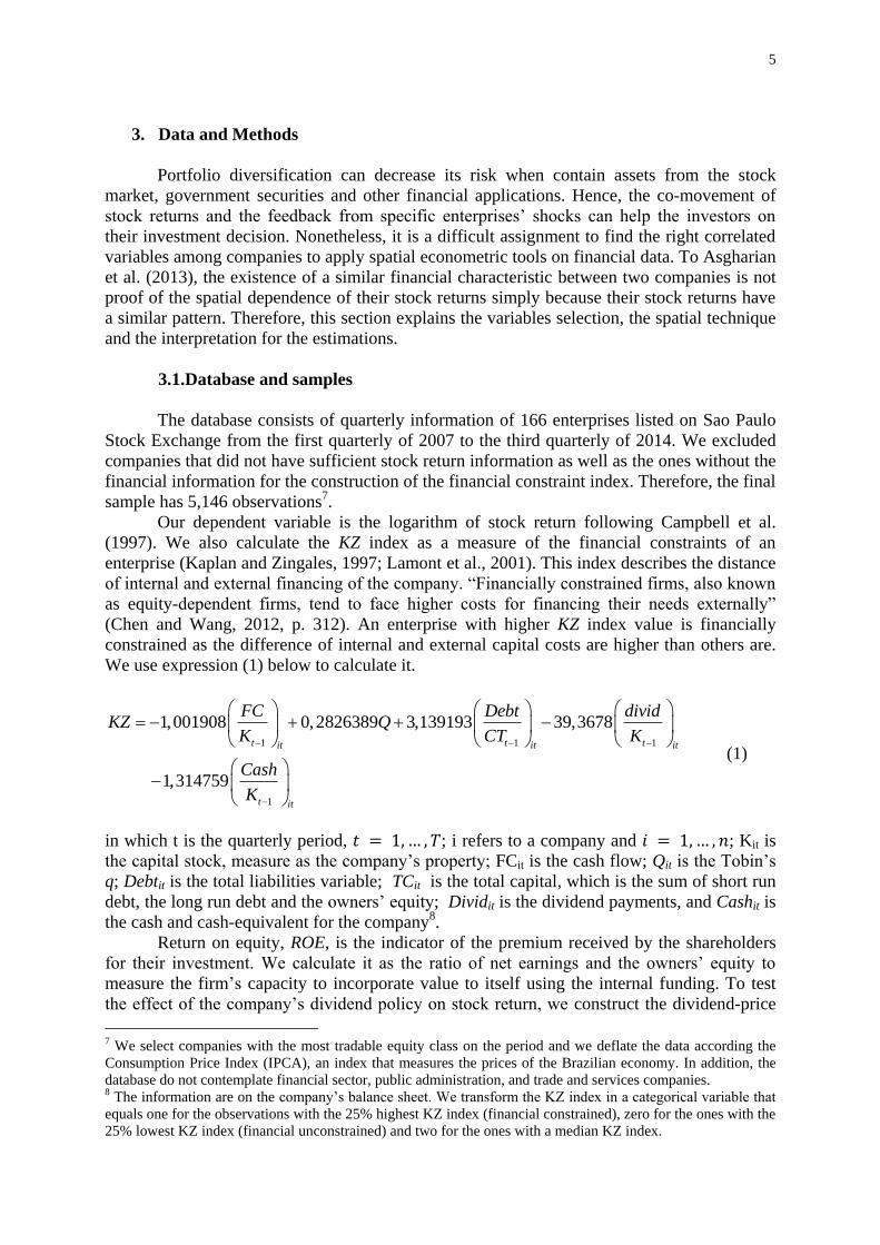
We use expression (1) below to calculate it.

1 1 1

1

1,001908 0,2

826389 3,139193

39,3678

1,31 9 5 47

t t tit it it

t it

FC Debt dividKZ Q

K CT K

Cash

K

(1)

in which t is the quarterly period, 𝑡 = 1, … , 𝑇; i refers to a company and 𝑖 = 1, … , 𝑛; Kit is

the capital stock, measure as the company’s property; FCit is the cash flow; Qit is the Tobin’s

q; Debtit is the total liabilities variable; TCit is the total capital, which is the sum of short run

debt, the long run debt and the owners’ equity; Dividit is the dividend payments, and Cashit is

the cash and cash-equivalent for the company8.

Return on equity, ROE, is the indicator of the premium received by the shareholders

for their investment. We calculate it as the ratio of net earnings and the owners’ equity to

measure the firm’s capacity to incorporate value to itself using the internal funding. To test

the effect of the company’s dividend policy on stock return, we construct the dividend-price

7 We select companies with the most tradable equity class on the period and we deflate the data according the

Consumption Price Index (IPCA), an index that measures the prices of the Brazilian economy. In addition, the

database do not contemplate financial sector, public administration, and trade and services companies. 8 The information are on the company’s balance sheet. We transform the KZ index in a categorical variable that

equals one for the observations with the 25% highest KZ index (financial constrained), zero for the ones with the

25% lowest KZ index (financial unconstrained) and two for the ones with a median KZ index.

6

ratio as the ratio of total dividend payment and total assets. We test if, considering the

Brazilian case, the dividend-policy irrelevance proposition of Miller and Modigliani is valid.

Golez (2014), for derivative market, suggests this variable is a proxy for expected stock return

when the expected dividend growth varies on time9.

To capture the investment opportunity, our last variable is the book-to-market ratio as

the ratio of the company’s book value and its market value. Leary and Roberts (2014) and

Cullen et al (2014) also use this variable to test for stock return or to understand the effects of

peer companies’ financial policies. To Leary and Roberts (2014, p.147), “the peer firm

average likely captures some variation in characteristics relevant for firm i’s capital structure

that is not capture by firm i’s own market-to-book ratio”. Therefore, we consider the inverse

of this variable as an investment opportunity measure.

Since the methodological procedures for spatial panel data using Stata must use a

balanced database, we consider two subsamples: (i) with a multivariate normal regression, we

use an imputation method to create a sample that accommodates arbitrary missing-value

patterns10

, and (ii) we reduce the sample to companies with all the valid information. For the

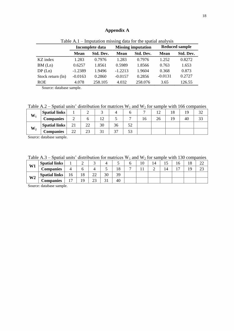
first subsample, the information on table A.1 reveals the method can be used without dramatic

modification on the average values. For the second subsample, we have 130 companies with

complete information for this period and we create a new spatial weight matrix with this

dimension. Table A.1 also describes the statistical summary of this sample. One can see some

modifications on the sample with a reduced number of companies. The first implication

would be higher values estimated on the spatial models, although the average stock returns

are similar to the original sample.

3.2.Econometric approach

Spatial econometric is a popular topic in regional economy, but its use on financial

applications is innovative. Its main idea is to understand how the spatial dependence affects

the dependent variable of a point in space relatively its value at another point in space

(Almeida, 2012). This argument is important as the existence of spatial dependence or

heterogeneity violates the Gauss-Markov assumptions making the estimation biased,

inconsistent, and inefficient (Anselin, 1988; Almeida, 2012).

The researcher can use geographical distance or any concept as a measure of distance

to the spatial weight matrix. Beck et al. (2006) apply spatial econometrics to social science

using an economic distance. Asgharian et al. (2013) test eight metrics of spatial weight

matrices also using economic distance to identify the contagion correlation in international

stock markets. Likewise, Arnold et al. (2013) and Suchecka and Laszkiewicz (2011) use non-

spatial criteria as a measure of correlation among stock returns11

.

Thus, the main concept of this technique is the construction of an adequate distance

matrix to understand the observed problem and to model the spatial dependence of the units.

If the researcher do not consider the spatial effects, an omission problem can affect the

estimations, leading to erroneous interpretations. Depending on the spatial correlation source,

Anselin (1988), LeSage and Pace (2009), and Elhorst (2014) establish a variety of spatial

regression structures and we select the Spatial Autoregressive Model (SAR) and the Spatial

Durbin Model (SDM)12

.

9 We select book-to-market and dividend-policy indicators as financial characteristics since Avramov (2002) use

them on a time series analysis. 10 This method uses an iterative Markov chain Monte Carlo (MCMC) method to impute missing values. 11 Some researchers on spatial econometrics without geographic measures are Chagas (2014), Conley and Dupor

(2003) and Beck et al. (2006). 12 For more detailed explanations about the other models, see LeSage and Pace (2009) and Elhorst (2014).

7

Formally, the spatial autoregressive models (SAR) contain, as an independent

variable, a spatial lag of the dependent variable which role is to incorporate a multidirectional

relationship between the spatial units. That means a spatial observation shock can feed back

other spatial observations through the spatial system (Anselin, 1988; LeSage and Pace, 2009).

Consequentially, this implies an endogeneity problem (from Wy), which makes the maximum

likelihood estimation model a method for unbiased and consistent parameters estimation. One

can write a SAR model as 𝑦 = 𝜌𝑊𝑦 + 𝑋𝛽 + 𝜀, with 𝑊𝑦 as the spatial lag of the dependent

variable.

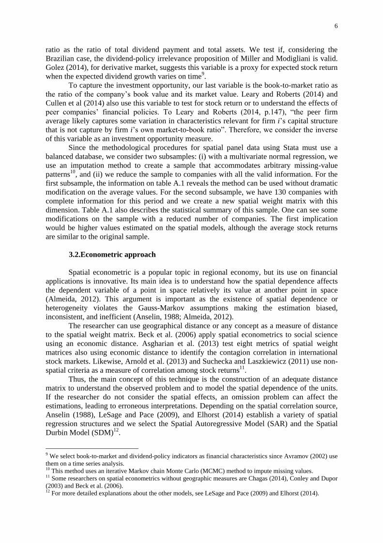
The spatial Durbin model (SDM) suggest the existence of a phenomenon that must use

a spatial lag dependent variable (Wy) and a spatial lag exploratory variable (WX). Elhorst

(2014) specify the panel data version of this model considering equation (2) in its matrix

form13

.

T T n

y I W y X I W X ι (2)

where W is a 𝑁 × 𝑁 spatial weight matrix, and ρ is a vector of the spatial dependence. y is a

vector with NT observations for the dependent variable; X is a 𝑁𝑇 × 𝐾 matrix with K

exploratory variables; β and θ are 𝐾 × 1 vector of parameters; ɩn is a 𝑁𝑇 × 𝑁 matrix

containing N individual constants; ε is a 𝑁𝑇 × 1 vector of idiosyncratic error terms; IT is the

identity matrix, and ⊗ is the Kronecker product.

Note from (2) that the Spatial Durbin Model has endogeneity problems and, therefore,

any estimation with ordinary least square is inconsistent. Thus, Anselin (1988), LeSage and

Pace (2009) and Elhorst (2014) recommend the maximum likelihood estimator or the

generalized method of moment as the estimation procedures that are unbiased and consistent.

We use the maximum likelihood estimator for each spatial weight matrix and its spatial

dependence. We consider a vector of 𝑁𝑇 observations consisting of quarterly stock returns

and a 𝑁𝑇 × 𝐾 matrix with K independent variables describe previously on subsection 3.1.

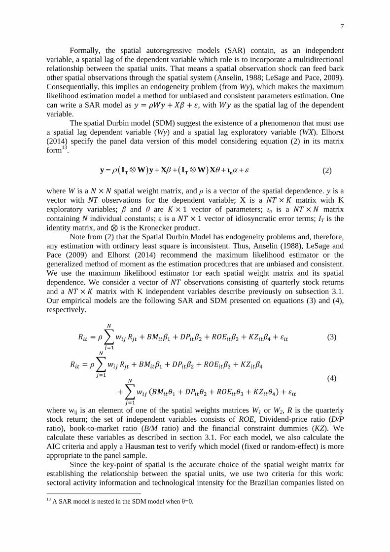
Our empirical models are the following SAR and SDM presented on equations (3) and (4),

respectively.

𝑅𝑖𝑡 = 𝜌 ∑𝑤𝑖𝑗

𝑁

𝑗=1

𝑅𝑗𝑡 + 𝐵𝑀𝑖𝑡𝛽1 + 𝐷𝑃𝑖𝑡𝛽2 + 𝑅𝑂𝐸𝑖𝑡𝛽3 + 𝐾𝑍𝑖𝑡𝛽4 + 𝜀𝑖𝑡 (3)

𝑅𝑖𝑡 = 𝜌 ∑𝑤𝑖𝑗

𝑁

𝑗=1

𝑅𝑗𝑡 + 𝐵𝑀𝑖𝑡𝛽1 + 𝐷𝑃𝑖𝑡𝛽2 + 𝑅𝑂𝐸𝑖𝑡𝛽3 + 𝐾𝑍𝑖𝑡𝛽4

+ ∑𝑤𝑖𝑗

𝑁

𝑗=1

(𝐵𝑀𝑖𝑡𝜃1 + 𝐷𝑃𝑖𝑡𝜃2 + 𝑅𝑂𝐸𝑖𝑡𝜃3 + 𝐾𝑍𝑖𝑡𝜃4) + 𝜀𝑖𝑡

(4)

where wij is an element of one of the spatial weights matrices W1 or W2, R is the quarterly

stock return; the set of independent variables consists of ROE, Dividend-price ratio (D/P

ratio), book-to-market ratio (B/M ratio) and the financial constraint dummies (KZ). We

calculate these variables as described in section 3.1. For each model, we also calculate the

AIC criteria and apply a Hausman test to verify which model (fixed or random-effect) is more

appropriate to the panel sample.

Since the key-point of spatial is the accurate choice of the spatial weight matrix for

establishing the relationship between the spatial units, we use two criteria for this work:

sectoral activity information and technological intensity for the Brazilian companies listed on

13 A SAR model is nested in the SDM model when θ=0.

8

the Sao Paulo Stock Exchange. Belonging to a specific sector is a simple form to construct a

proximity matrix14

. We consider the companies spatial correlated if they operate on the same

activity sector or if they operate in the same technological sector. This choice standardize the

spatial weight variable between periods and smooth the Elhorst (2014) estimation procedure

for panel data.

Therefore, we name the spatial weight matrix with sectoral proximity, as W1, and the

second matrix with the technological intensity, as W2, both are time invariant. The final

spatial weight matrices are quadratic and row-normalized. Its elements establish a binary

relationship among spatial units (companies). We suppose company i as an influential factor

on company j if both belong to the same activity sector and attribute a spatial weight equal to

𝜔𝑖,𝑗 = 𝜔𝑗,𝑖 = 1 , otherwise the weights are 𝜔𝑖,𝑗 = 𝜔𝑗,𝑖 = 0. In spatial econometrics, we

cannot say one spatial unit is correlated to itself, thus, 𝜔𝑖,𝑖 = 𝜔𝑗,𝑗 = 0, which indicates the

main diagonal elements are equal to zero. These matrices allow a variability to the number of

companies as competitors or cooperators accordingly the companies included on the database

and its respective sector of activity or technological intensity.

To interpret the parameters correctly, one cannot use the same principal of traditional

econometrics. On spatial econometric models, the interpretation is fundamental. Using the

reduced form of the model (2), since the SAR model is nested in it, we can find the average

effects of the spatial estimations. This form shows the effects produced on company i because

of changes on the other companies as a result of their spatial relationship. LeSage and Pace

(2009, p. 33) affirm “the parameters estimates contain a wealth of information on

relationships among the observations”.

Any change on an observation’s exploratory variable can affect all the spatial units

direct or indirectly. Thus, any interpretation has to use marginal effects for the partial

derivatives. LeSage and Pace (2009) and Elhorst (2014) suggest two types of marginal effects

known as direct and indirect effects. The first ones measure the impact of a change on an

independent variable k for company i on the dependent variable of the same company. The

indirect effects results of the change on an independent variable k for company j on the

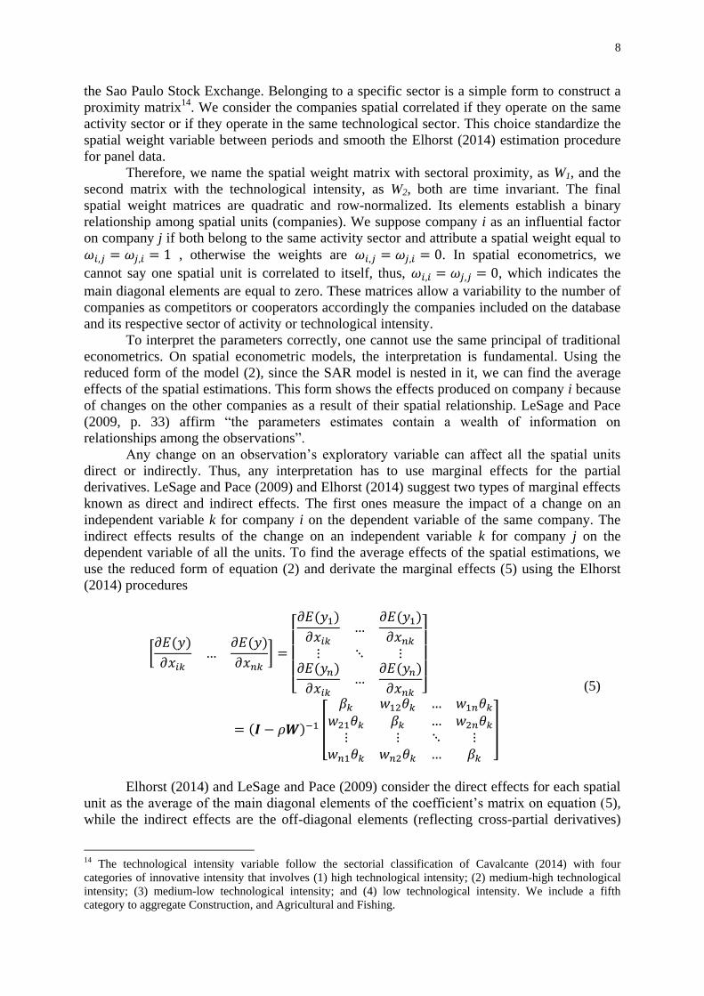
dependent variable of all the units. To find the average effects of the spatial estimations, we

use the reduced form of equation (2) and derivate the marginal effects (5) using the Elhorst

(2014) procedures

[𝜕𝐸(𝑦)

𝜕𝑥𝑖𝑘…

𝜕𝐸(𝑦)

𝜕𝑥𝑛𝑘] =

[ 𝜕𝐸(𝑦1)

𝜕𝑥𝑖𝑘…

𝜕𝐸(𝑦1)

𝜕𝑥𝑛𝑘

⋮ ⋱ ⋮𝜕𝐸(𝑦𝑛)

𝜕𝑥𝑖𝑘…

𝜕𝐸(𝑦𝑛)

𝜕𝑥𝑛𝑘 ]

= (𝑰 − 𝜌𝑾)−1 [

𝛽𝑘 𝑤12𝜃𝑘 … 𝑤1𝑛𝜃𝑘

𝑤21𝜃𝑘 𝛽𝑘 … 𝑤2𝑛𝜃𝑘

⋮ ⋮ ⋱ ⋮𝑤𝑛1𝜃𝑘 𝑤𝑛2𝜃𝑘 … 𝛽𝑘

]

(5)

Elhorst (2014) and LeSage and Pace (2009) consider the direct effects for each spatial

unit as the average of the main diagonal elements of the coefficient’s matrix on equation (5),

while the indirect effects are the off-diagonal elements (reflecting cross-partial derivatives)

14 The technological intensity variable follow the sectorial classification of Cavalcante (2014) with four

categories of innovative intensity that involves (1) high technological intensity; (2) medium-high technological

intensity; (3) medium-low technological intensity; and (4) low technological intensity. We include a fifth

category to aggregate Construction, and Agricultural and Fishing.

9

from each row. The authors suggest the summarized measure of these average marginal

effects to understand the variable behavior by using the following expressions for the average

direct, average indirect and average total effects

Average direct impact: refers to the change on the ith

spatial unit of xk on yi,

(company’s own stock return), comprehending the main diagonal elements of

the matrix in (5). That is 𝑛−1𝑡𝑟[(𝑰𝑵𝑻 − 𝜌(𝑰𝑻 ⊗ 𝑾))−1[𝑰𝑵𝛽 + (𝑰𝑻 ⊗ 𝑾)𝜃]; Average total impact: refers to the variation of only one spatial unit on all the

spatial units. We calculate 𝑛−1𝜾𝒏′ [(𝑰𝑵𝑻 − 𝜌(𝑰𝑻 ⊗ 𝑾))−1[𝑰𝑵𝛽 + (𝑰𝑻 ⊗

𝑾)𝜃]𝜾𝒏; and

Average indirect impact is the difference between the total average effect and

the average direct effect and represents the feedback impacts on the global and

local spatial system. It is all the off-diagonal elements on equation (5).

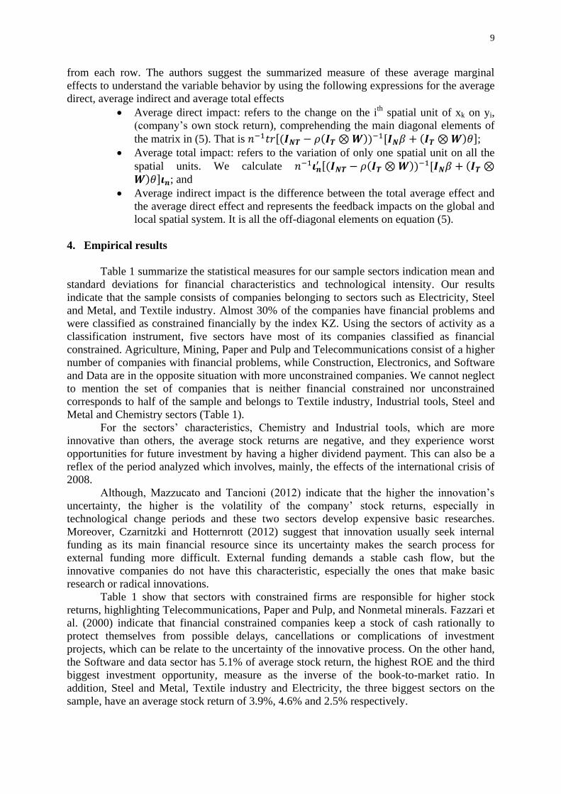
4. Empirical results

Table 1 summarize the statistical measures for our sample sectors indication mean and

standard deviations for financial characteristics and technological intensity. Our results

indicate that the sample consists of companies belonging to sectors such as Electricity, Steel

and Metal, and Textile industry. Almost 30% of the companies have financial problems and

were classified as constrained financially by the index KZ. Using the sectors of activity as a

classification instrument, five sectors have most of its companies classified as financial

constrained. Agriculture, Mining, Paper and Pulp and Telecommunications consist of a higher

number of companies with financial problems, while Construction, Electronics, and Software

and Data are in the opposite situation with more unconstrained companies. We cannot neglect

to mention the set of companies that is neither financial constrained nor unconstrained

corresponds to half of the sample and belongs to Textile industry, Industrial tools, Steel and

Metal and Chemistry sectors (Table 1).

For the sectors’ characteristics, Chemistry and Industrial tools, which are more

innovative than others, the average stock returns are negative, and they experience worst

opportunities for future investment by having a higher dividend payment. This can also be a

reflex of the period analyzed which involves, mainly, the effects of the international crisis of

2008.

Although, Mazzucato and Tancioni (2012) indicate that the higher the innovation’s

uncertainty, the higher is the volatility of the company’ stock returns, especially in

technological change periods and these two sectors develop expensive basic researches.

Moreover, Czarnitzki and Hotternrott (2012) suggest that innovation usually seek internal

funding as its main financial resource since its uncertainty makes the search process for

external funding more difficult. External funding demands a stable cash flow, but the

innovative companies do not have this characteristic, especially the ones that make basic

research or radical innovations.

Table 1 show that sectors with constrained firms are responsible for higher stock

returns, highlighting Telecommunications, Paper and Pulp, and Nonmetal minerals. Fazzari et

al. (2000) indicate that financial constrained companies keep a stock of cash rationally to

protect themselves from possible delays, cancellations or complications of investment

projects, which can be relate to the uncertainty of the innovative process. On the other hand,

the Software and data sector has 5.1% of average stock return, the highest ROE and the third

biggest investment opportunity, measure as the inverse of the book-to-market ratio. In

addition, Steel and Metal, Textile industry and Electricity, the three biggest sectors on the

sample, have an average stock return of 3.9%, 4.6% and 2.5% respectively.

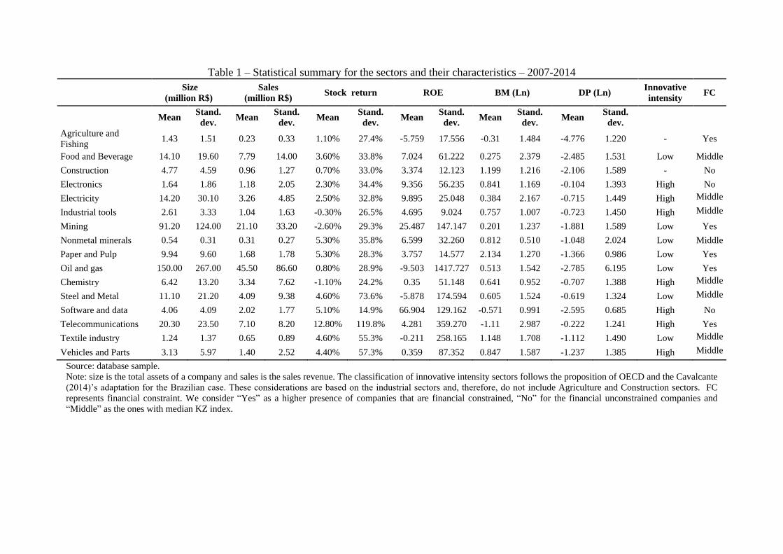
Table 1 – Statistical summary for the sectors and their characteristics – 2007-2014

Size

(million R$)

Sales

(million R$) Stock return ROE BM (Ln) DP (Ln)

Innovative

intensity FC

Mean

Stand.

dev. Mean

Stand.

dev. Mean

Stand.

dev. Mean

Stand.

dev. Mean

Stand.

dev. Mean

Stand.

dev.

Agriculture and

Fishing 1.43 1.51 0.23 0.33 1.10% 27.4% -5.759 17.556 -0.31 1.484 -4.776 1.220 - Yes

Food and Beverage 14.10 19.60 7.79 14.00 3.60% 33.8% 7.024 61.222 0.275 2.379 -2.485 1.531 Low Middle

Construction 4.77 4.59 0.96 1.27 0.70% 33.0% 3.374 12.123 1.199 1.216 -2.106 1.589 - No

Electronics 1.64 1.86 1.18 2.05 2.30% 34.4% 9.356 56.235 0.841 1.169 -0.104 1.393 High No

Electricity 14.20 30.10 3.26 4.85 2.50% 32.8% 9.895 25.048 0.384 2.167 -0.715 1.449 High Middle

Industrial tools 2.61 3.33 1.04 1.63 -0.30% 26.5% 4.695 9.024 0.757 1.007 -0.723 1.450 High Middle

Mining 91.20 124.00 21.10 33.20 -2.60% 29.3% 25.487 147.147 0.201 1.237 -1.881 1.589 Low Yes

Nonmetal minerals 0.54 0.31 0.31 0.27 5.30% 35.8% 6.599 32.260 0.812 0.510 -1.048 2.024 Low Middle

Paper and Pulp 9.94 9.60 1.68 1.78 5.30% 28.3% 3.757 14.577 2.134 1.270 -1.366 0.986 Low Yes

Oil and gas 150.00 267.00 45.50 86.60 0.80% 28.9% -9.503 1417.727 0.513 1.542 -2.785 6.195 Low Yes

Chemistry 6.42 13.20 3.34 7.62 -1.10% 24.2% 0.35 51.148 0.641 0.952 -0.707 1.388 High Middle

Steel and Metal 11.10 21.20 4.09 9.38 4.60% 73.6% -5.878 174.594 0.605 1.524 -0.619 1.324 Low Middle

Software and data 4.06 4.09 2.02 1.77 5.10% 14.9% 66.904 129.162 -0.571 0.991 -2.595 0.685 High No

Telecommunications 20.30 23.50 7.10 8.20 12.80% 119.8% 4.281 359.270 -1.11 2.987 -0.222 1.241 High Yes

Textile industry 1.24 1.37 0.65 0.89 4.60% 55.3% -0.211 258.165 1.148 1.708 -1.112 1.490 Low Middle

Vehicles and Parts 3.13 5.97 1.40 2.52 4.40% 57.3% 0.359 87.352 0.847 1.587 -1.237 1.385 High Middle

Source: database sample.

Note: size is the total assets of a company and sales is the sales revenue. The classification of innovative intensity sectors follows the proposition of OECD and the Cavalcante

(2014)’s adaptation for the Brazilian case. These considerations are based on the industrial sectors and, therefore, do not include Agriculture and Construction sectors. FC

represents financial constraint. We consider “Yes” as a higher presence of companies that are financial constrained, “No” for the financial unconstrained companies and

“Middle” as the ones with median KZ index.

Size and sales can illustrate the importance of each branch of activity. One can see

that, using this sample, the companies of Oil and gas and Mining sectors are the bigger ones

and are responsible for the higher sales revenue of the sample but have financial difficulties

for our financial constraint index. On the other hand, Nonmetal minerals, Textile Industry,

Electronics and Agriculture and Fishing have smaller size relatively to the other sectors. For

the sales revenue, Chemistry and Mining have the lowest stock return but, surprisingly, have a

higher level of sales revenue on the period possibly as a response to the commodities’

international prices. On the other hand, the other sectors have a lower level of this variable

especially Telecommunications and Nonmetal Minerals, which have some type of financial

restrictions (Table 1).

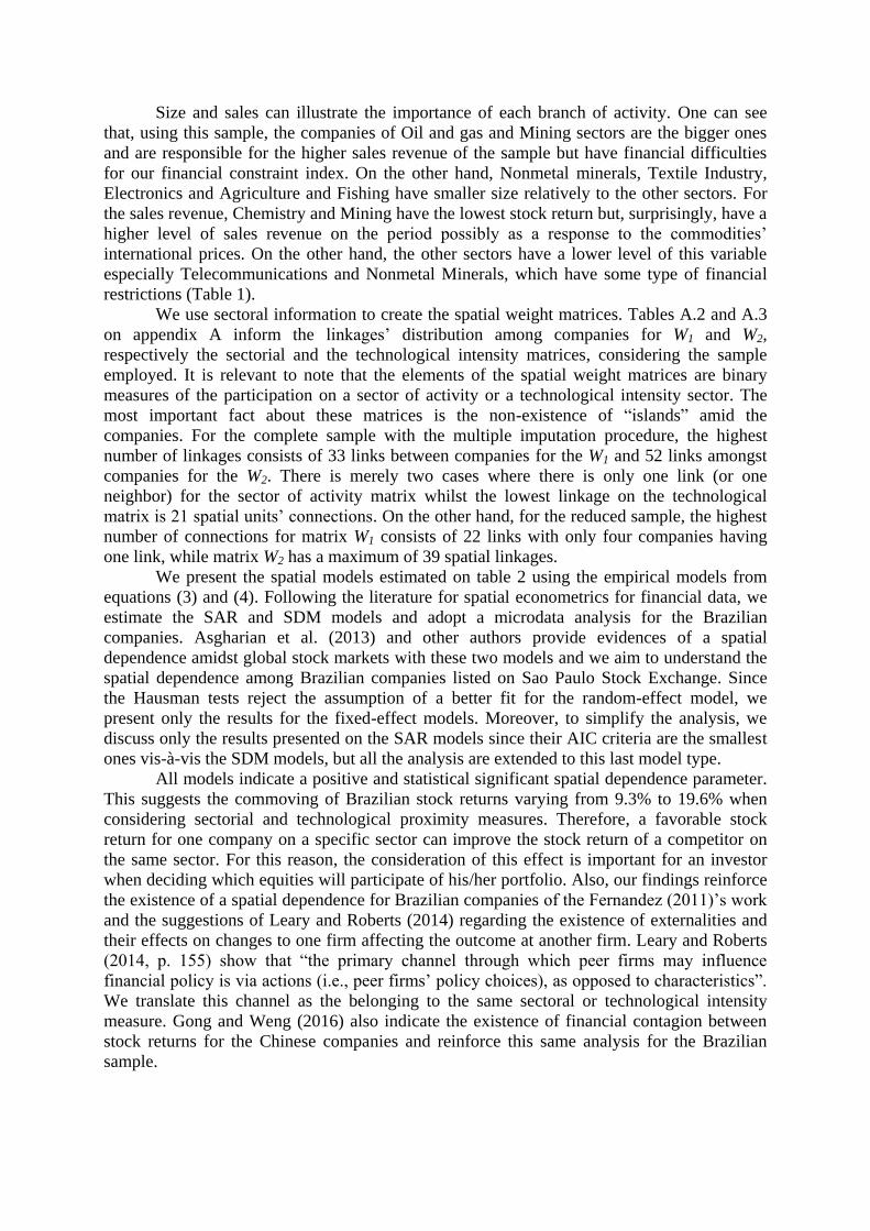
We use sectoral information to create the spatial weight matrices. Tables A.2 and A.3

on appendix A inform the linkages’ distribution among companies for W1 and W2,

respectively the sectorial and the technological intensity matrices, considering the sample

employed. It is relevant to note that the elements of the spatial weight matrices are binary

measures of the participation on a sector of activity or a technological intensity sector. The

most important fact about these matrices is the non-existence of “islands” amid the

companies. For the complete sample with the multiple imputation procedure, the highest

number of linkages consists of 33 links between companies for the W1 and 52 links amongst

companies for the W2. There is merely two cases where there is only one link (or one

neighbor) for the sector of activity matrix whilst the lowest linkage on the technological

matrix is 21 spatial units’ connections. On the other hand, for the reduced sample, the highest

number of connections for matrix W1 consists of 22 links with only four companies having

one link, while matrix W2 has a maximum of 39 spatial linkages.

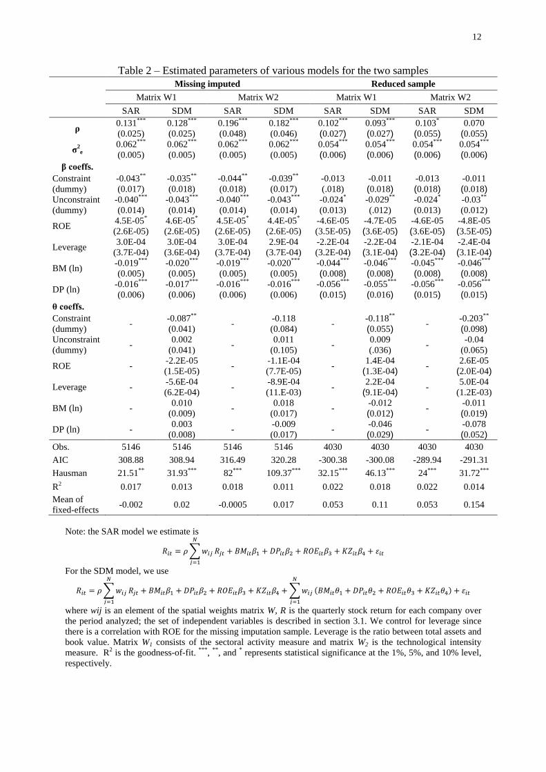
We present the spatial models estimated on table 2 using the empirical models from

equations (3) and (4). Following the literature for spatial econometrics for financial data, we

estimate the SAR and SDM models and adopt a microdata analysis for the Brazilian

companies. Asgharian et al. (2013) and other authors provide evidences of a spatial

dependence amidst global stock markets with these two models and we aim to understand the

spatial dependence among Brazilian companies listed on Sao Paulo Stock Exchange. Since

the Hausman tests reject the assumption of a better fit for the random-effect model, we

present only the results for the fixed-effect models. Moreover, to simplify the analysis, we

discuss only the results presented on the SAR models since their AIC criteria are the smallest

ones vis-à-vis the SDM models, but all the analysis are extended to this last model type.

All models indicate a positive and statistical significant spatial dependence parameter.

This suggests the commoving of Brazilian stock returns varying from 9.3% to 19.6% when

considering sectorial and technological proximity measures. Therefore, a favorable stock

return for one company on a specific sector can improve the stock return of a competitor on

the same sector. For this reason, the consideration of this effect is important for an investor

when deciding which equities will participate of his/her portfolio. Also, our findings reinforce

the existence of a spatial dependence for Brazilian companies of the Fernandez (2011)’s work

and the suggestions of Leary and Roberts (2014) regarding the existence of externalities and

their effects on changes to one firm affecting the outcome at another firm. Leary and Roberts

(2014, p. 155) show that “the primary channel through which peer firms may influence

financial policy is via actions (i.e., peer firms’ policy choices), as opposed to characteristics”.

We translate this channel as the belonging to the same sectoral or technological intensity

measure. Gong and Weng (2016) also indicate the existence of financial contagion between

stock returns for the Chinese companies and reinforce this same analysis for the Brazilian

sample.

12

Table 2 – Estimated parameters of various models for the two samples

Missing imputed Reduced sample

Matrix W1 Matrix W2 Matrix W1 Matrix W2

SAR SDM SAR SDM SAR SDM SAR SDM

ρ 0.131***

(0.025)

0.128***

(0.025)

0.196***

(0.048)

0.182***

(0.046)

0.102*** (0.027)

0.093***

(0.027) 0.103* (0.055)

0.070 (0.055)

σ2e

0.062***

(0.005)

0.062***

(0.005)

0.062***

(0.005)

0.062***

(0.005)

0.054*** (0.006)

0.054*** (0.006)

0.054*** (0.006)

0.054*** (0.006)

β coeffs.

Constraint

(dummy)

-0.043**

(0.017)

-0.035**

(0.018)

-0.044**

(0.018)

-0.039**

(0.017)

-0.013

(.018)

-0.011 (0.018)

-0.013 (0.018)

-0.011 (0.018)

Unconstraint

(dummy)

-0.040***

(0.014)

-0.043***

(0.014)

-0.040***

(0.014)

-0.043***

(0.014)

-0.024*

(0.013)

-0.029**

(.012)

-0.024*

(0.013)

-0.03**

(0.012)

ROE 4.5E-05*

(2.6E-05)

4.6E-05*

(2.6E-05)

4.5E-05*

(2.6E-05)

4.4E-05*

(2.6E-05)

-4.6E-05

(3.5E-05)

-4.7E-05 (3.6E-05)

-4.6E-05 (3.6E-05)

-4.8E-05 (3.5E-05)

Leverage 3.0E-04

(3.7E-04)

3.0E-04

(3.6E-04)

3.0E-04

(3.7E-04)

2.9E-04

(3.7E-04)

-2.2E-04

(3.2E-04)

-2.2E-04 (3.1E-04)

-2.1E-04 (3.2E-04)

-2.4E-04 (3.1E-04)

BM (ln) -0.019***

(0.005)

-0.020***

(0.005)

-0.019***

(0.005)

-0.020***

(0.005)

-0.044*** (0.008)

-0.046***

(0.008) -0.045*** (0.008)

-0.046*** (0.008)

DP (ln) -0.016***

(0.006)

-0.017***

(0.006)

-0.016***

(0.006)

-0.016***

(0.006)

-0.056*** (0.015)

-0.055***

(0.016) -0.056*** (0.015)

-0.056*** (0.015)

θ coeffs.

Constraint

(dummy) -

-0.087**

(0.041) -

-0.118

(0.084) -

-0.118** (0.055)

- -0.203** (0.098)

Unconstraint

(dummy) -

0.002

(0.041) -

0.011

(0.105) -

0.009

(.036) -

-0.04

(0.065)

ROE - -2.2E-05

(1.5E-05) -

-1.1E-04

(7.7E-05) -

1.4E-04 (1.3E-04)

- 2.6E-05

(2.0E-04)

Leverage - -5.6E-04

(6.2E-04) -

-8.9E-04

(11.E-03) -

2.2E-04 (9.1E-04)

- 5.0E-04

(1.2E-03)

BM (ln) - 0.010

(0.009) -

0.018

(0.017) -

-0.012 (0.012)

- -0.011 (0.019)

DP (ln) - 0.003

(0.008) -

-0.009

(0.017) -

-0.046 (0.029)

- -0.078 (0.052)

Obs. 5146 5146 5146 5146 4030 4030 4030 4030

AIC 308.88 308.94 316.49 320.28 -300.38 -300.08 -289.94 -291.31

Hausman 21.51** 31.93*** 82*** 109.37*** 32.15*** 46.13*** 24*** 31.72***

R2 0.017 0.013 0.018 0.011 0.022 0.018 0.022 0.014

Mean of

fixed-effects -0.002 0.02 -0.0005 0.017 0.053 0.11 0.053 0.154

Note: the SAR model we estimate is

𝑅𝑖𝑡 = 𝜌 ∑𝑤𝑖𝑗

𝑁

𝑗=1

𝑅𝑗𝑡 + 𝐵𝑀𝑖𝑡𝛽1 + 𝐷𝑃𝑖𝑡𝛽2 + 𝑅𝑂𝐸𝑖𝑡𝛽3 + 𝐾𝑍𝑖𝑡𝛽4 + 𝜀𝑖𝑡

For the SDM model, we use

𝑅𝑖𝑡 = 𝜌 ∑𝑤𝑖𝑗

𝑁

𝑗=1

𝑅𝑗𝑡 + 𝐵𝑀𝑖𝑡𝛽1 + 𝐷𝑃𝑖𝑡𝛽2 + 𝑅𝑂𝐸𝑖𝑡𝛽3 + 𝐾𝑍𝑖𝑡𝛽4 + ∑𝑤𝑖𝑗

𝑁

𝑗=1

(𝐵𝑀𝑖𝑡𝜃1 + 𝐷𝑃𝑖𝑡𝜃2 + 𝑅𝑂𝐸𝑖𝑡𝜃3 + 𝐾𝑍𝑖𝑡𝜃4) + 𝜀𝑖𝑡

where wij is an element of the spatial weights matrix W, R is the quarterly stock return for each company over

the period analyzed; the set of independent variables is described in section 3.1. We control for leverage since

there is a correlation with ROE for the missing imputation sample. Leverage is the ratio between total assets and

book value. Matrix W1 consists of the sectoral activity measure and matrix W2 is the technological intensity

measure. R2 is the goodness-of-fit. ***, **, and * represents statistical significance at the 1%, 5%, and 10% level,

respectively.

13

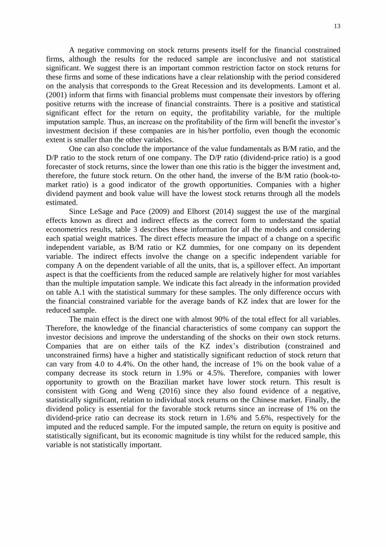
A negative commoving on stock returns presents itself for the financial constrained

firms, although the results for the reduced sample are inconclusive and not statistical

significant. We suggest there is an important common restriction factor on stock returns for

these firms and some of these indications have a clear relationship with the period considered

on the analysis that corresponds to the Great Recession and its developments. Lamont et al.

(2001) inform that firms with financial problems must compensate their investors by offering

positive returns with the increase of financial constraints. There is a positive and statistical

significant effect for the return on equity, the profitability variable, for the multiple

imputation sample. Thus, an increase on the profitability of the firm will benefit the investor’s

investment decision if these companies are in his/her portfolio, even though the economic

extent is smaller than the other variables.

One can also conclude the importance of the value fundamentals as B/M ratio, and the

D/P ratio to the stock return of one company. The D/P ratio (dividend-price ratio) is a good

forecaster of stock returns, since the lower than one this ratio is the bigger the investment and,

therefore, the future stock return. On the other hand, the inverse of the B/M ratio (book-to-

market ratio) is a good indicator of the growth opportunities. Companies with a higher

dividend payment and book value will have the lowest stock returns through all the models

estimated.

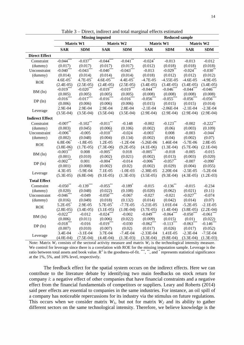
Since LeSage and Pace (2009) and Elhorst (2014) suggest the use of the marginal

effects known as direct and indirect effects as the correct form to understand the spatial

econometrics results, table 3 describes these information for all the models and considering

each spatial weight matrices. The direct effects measure the impact of a change on a specific

independent variable, as B/M ratio or KZ dummies, for one company on its dependent

variable. The indirect effects involve the change on a specific independent variable for

company A on the dependent variable of all the units, that is, a spillover effect. An important

aspect is that the coefficients from the reduced sample are relatively higher for most variables

than the multiple imputation sample. We indicate this fact already in the information provided

on table A.1 with the statistical summary for these samples. The only difference occurs with

the financial constrained variable for the average bands of KZ index that are lower for the

reduced sample.

The main effect is the direct one with almost 90% of the total effect for all variables.

Therefore, the knowledge of the financial characteristics of some company can support the

investor decisions and improve the understanding of the shocks on their own stock returns.

Companies that are on either tails of the KZ index’s distribution (constrained and

unconstrained firms) have a higher and statistically significant reduction of stock return that

can vary from 4.0 to 4.4%. On the other hand, the increase of 1% on the book value of a

company decrease its stock return in 1.9% or 4.5%. Therefore, companies with lower

opportunity to growth on the Brazilian market have lower stock return. This result is

consistent with Gong and Weng (2016) since they also found evidence of a negative,

statistically significant, relation to individual stock returns on the Chinese market. Finally, the

dividend policy is essential for the favorable stock returns since an increase of 1% on the

dividend-price ratio can decrease its stock return in 1.6% and 5.6%, respectively for the

imputed and the reduced sample. For the imputed sample, the return on equity is positive and

statistically significant, but its economic magnitude is tiny whilst for the reduced sample, this

variable is not statistically important.

14

Table 3 – Direct, indirect and total marginal effects estimated

Missing imputed Reduced sample

Matrix W1 Matrix W2 Matrix W1 Matrix W2

SAR SDM SAR SDM SAR SDM SAR SDM

Direct Effect

Constraint

(dummy)

-0.044***

(0.017)

-0.037**

(0.017)

-0.044***

(0.017)

-0.041**

(0.017)

-0.024*

(0.012)

-0.013

(0.018)

-0.013

(0.018)

-0.012

(0.018)

Unconstraint

(dummy)

-0.040***

(0.014)

-0.043***

(0.014)

-0.040***

(0.014)

-0.043***

(0.014)

-0.013

(0.018)

-0.029**

(0.012)

-0.024**

(0.012)

-0.030**

(0.012)

ROE 4.6E-05*

(2.4E-05)

4.7E-05*

(2.5E-05)

4.6E-05***

(2.4E-05)

4.4E-05*

(2.5E-05)

-4.7E-05

(3.4E-05)

-4.55E-05

(3.4E-05)

-4.6E-05

(3.4E-05)

-4.9E-05

(3.4E-05)

BM (ln) -0.019***

(0.005)

-0.020***

(0.005)

-0.019***

(0.005)

-0.019***

(0.005)

-0.044***

(0.008)

-0.046***

(0.008)

-0.044***

(0.008)

-0.046***

(0.008)

DP (ln) -0.016***

(0.006)

-0.017***

(0.006)

-0.016***

(0.006)

-0.016***

(0.006)

-0.056***

(0.015)

-0.055***

(0.015)

-0.056***

(0.015)

-0.056***

(0.014)

Leverage 2.9E-04

(3.5E-04)

2.9E-04

(3.5E-04)

2.9E-04

(3.5E-04)

2.8E-04

(3.5E-04)

-2.1E-04

(2.9E-04)

-2.06E-04

(2.9E-04)

-2.1E-04

(2.9E-04)

-2.3E-04

(2.9E-04)

Indirect Effect

Constraint

(dummy)

-0.007**

(0.003)

-0.102**

(0.045)

-0.011**

(0.006)

-0.148

(0.106)

-0.002

(0.002)

-0.123**

(0.06)

-0.002

(0.003)

-0.222**

(0.109)

Unconstraint

(dummy)

-0.006**

(0.002)

-0.005

(0.048)

-0.010**

(0.004)

-0.024

(0.134)

-0.003*

(0.002)

0.008

(0.04)

-0.003

(0.002)

-0.044*

(0.07)

ROE 6.8E-06*

(3.8E-06)

-1.8E-05

(1.7E-05)

1.2E-05

(7.3E-06)

-1.2E-04

(9.2E-05)

-5.26E-06

(4.1E-06)

1.46E-04

(1.3E-04)

-5.7E-06

(5.7E-06)

2.8E-05

(2.1E-04)

BM (ln) -0.003***

(0.001)

0.008

(0.010)

-0.005**

(0.002)

0.018

(0.021)

-0.005***

(0.002)

-0.018

(0.013)

-0.005

(0.003)

-0.015

(0.020)

DP (ln) -0.002***

(0.001)

0.001

(0.008)

-0.004**

(0.002)

-0.014

(0.02)

-0.006**

(0.002)

-0.057**

(0.029)

-0.007

(0.004)

-0.090*

(0.055)

Leverage 4.3E-05

(5.3E-05)

-5.9E-04

(6.8E-04)

7.1E-05

(9.1E-05)

-1.0E-03

(1.3E-03)

-2.38E-05

(3.5E-05)

2.20E-04

(9.3E-04)

-2.5E-05

(4.3E-05)

-5.2E-04

(1.2E-03)

Total Effect

Constraint

(dummy)

-0.050**

(0.020)

-0.139***

(0.048)

-0.055**

(0.022)

-0.189*

(0.108)

-0.015

(0.020)

-0.136**

(0.062)

-0.015

(0.021)

-0.234

(0.11)

Unconstraint

(dummy)

-0.046***

(0.016)

-0.049

(0.049)

-0.050***

(0.018)

-0.067

(0.132)

-0.027

(0.014)

-0.021

(0.042)

-0.027**

(0.014)

-0.074

(0.07)

ROE 5.2E-05*

(2.8E-05)

2.9E-05

(3.4E-05)

5.7E-05*

(3.1E-05)

-7.7E-05

(1.0E-04)

-5.21E-05

(3.7E-05)

1.01E-04

(1.4E-04)

-5.2E-05

(3.8E-05)

-2.1E-05

(2.2E-04)

BM (ln) -0.022***

(0.006)

-0.012

(0.011)

-0.024***

(0.006)

-0.002

(0.022)

-0.049***

(0.009)

-0.064***

(0.015)

-0.050***

(0.01)

-0.061***

(0.022)

DP (ln) -0.018***

(0.007)

-0.016

(0.010)

-0.019***

(0.007)

-0.030

(0.02)

-0.062***

(0.017)

-0.113***

(0.026)

-0.063***

(0.017)

-0.146***

(0.052)

Leverage 3.4E-04

(4.0E-04)

-3.1E-04

(7.5E-04)

3.7E-04

(4.4E-04)

-7.4E-04

(1.3E-03)

-2.33E-04

(3.3E-04)

1.41E-05

(9.8E-04)

-2.3E-04

(3.3E-04)

-7.5E-04

(1.3E-03)

Note: Matrix W1 consists of the sectoral activity measure and matrix W2 is the technological intensity measure.

We control for leverage since there is a correlation with ROE for the missing imputation sample. Leverage is the

ratio between total assets and book value. R2 is the goodness-of-fit. ***, **, and * represents statistical significance

at the 1%, 5%, and 10% level, respectively.

The feedback effect for the spatial system occurs on the indirect effects. Here we can

contribute to the literature debate by identifying two main feedbacks on stock return for

company i: a negative effect of other companies that have financial constraints and a negative

effect from the financial fundamentals of competitors or suppliers. Leary and Roberts (2014)

said peer effects are essential to companies in the same industries. For instance, an oil spill of

a company has noticeable repercussions for its industry via the stimulus on future regulations.

This occurs when we consider matrix W1, but not for matrix W2 and its ability to gather

different sectors on the same technological intensity. Therefore, we believe knowledge is the

15

key to capture better stock returns for the investors. If a company belongs to a baseline group

consisting of companies that have financial problems, then it may contribute to decrease the

stock return of a competitor on 0.7% for the imputed sample. Already, for the technological

proximity, we conclude that financial problem can be a response for the innovative

investment process and, hence, will bring lower opportunities to growth and lower stock

returns for the short run (a decrease of 1.1% for the imputed sample). The unconstrained

companies have the same problems but with lower values since the period analyzed is critical

to the Brazilian companies listed on Sao Paulo Stock Exchange.

For the second type of feedback, competitors with a higher dividend payment can

negatively influence the stock returns of the companies in the baseline group since the

investor can see the relationship amongst them as an indicator of lower expected stock returns

for the group. This is also the conclusion we make for the B/M ratio. Competitors with a

higher book value – or that lost some market value on the period – can penalize the baseline

group with a decrease from 0.3% to 0.5% on stock returns as an indication of the decrease in

opportunity growth. The reduced sample is responsible for the biggest feedback reductions of

the stock return in baseline groups. This means that 130 companies on the reduced sample,

when aggregate by branch of activity (matrix W1), are more susceptible to have a 0.5% or

0.64% decrease in their stock return if the sectoral group is known as a higher dividend

distributor.

5. Conclusions

In this paper, we have tested for spatial dependence in a panel of 166 Brazilian

companies over the period of 2007-2014. We use two economic distance measures for the

construction of the spatial weight matrices: branch of activity and technological intensity of

the sector. To our knowledge, this is the first time the spatial econometrics is applied to micro

econometric analysis of financial data in Brazil. International empirical literature has shown

the existence of spatial dependence on financial analysis and its importance for the

construction of portfolios.

Our results indicate a spatial dependence in the Brazilian companies listed on the stock

exchange for two distance measures and its positive effect on the stock returns. Hence, the

knowledge of boom periods for the competitors can positively improve the stock return of a

company in the same baseline group. Therefore, companies in the same branch of activity (or

the same technological intensity of it sector) can benefit themselves by the good phase of

competitors, obtaining positively greater stock returns not only for the maintaining of their

financial foundations, but by the interaction with the companies of their group.

Contrariwise, the B/M ratio and the D/P ratio are important financial fundamentals

that need consideration by the investor if a higher stock return is their main decision. This is

also an indication of the risk of a portfolio behavior with the companies from the same group.

Our results reveal that companies with more investment opportunities and less dividend

payment have increases on their stock returns as a result of the spillover of companies with

the same characteristics.

We have two main limitations: the construction of the spatial weight matrices since it

is difficult to create a measure of spatial dependence for financial data, and the period

considered for the analysis. The international crisis from 2008/2009 had great influence on the

stock returns for the Brazilian companies and was able to reduce the Brazilian capital

market’s returns for either the financial constrained and unconstrained companies counted on

this paper. We suggest future studies seek different strategies to identify competitors and

customer/supplier relationships amongst other industries and the inclusion of an extended

period to understand the companies listed on Sao Paulo Stock Exchange.

16

References

Almeida, E. (2012). Econometria Espacial Aplicada. Campinas: Editora Alínea, 498p.

Anselin, L. (1988). Spatial Econometrics: methods and models. Boston: Kluwer Academic.

Arnold, M.; Stahlberg, S.; Wied, D. (2013) Modelling different kinds of spatial dependence in

stock return. Empirical Economics, 44 (2): 761-774.

Asgharian, H.; Hess, W.; Liu, L. (2013). A spatial analysis of international stock market

linkages. Journal of Banking & Finance, v. 37, pp. 4738-4754.

Beck, N.; Gleditsch, K.S.; Beardsley, K. (2006). Space is more than geography: using spatial

econometrics in the study of political economy. International Studies Quarterly, 50: 27-44.

Campbell, J.Y.; Lo, A.W.; Mackinlay, A.C. (1997). The Econometrics of Financial

Markets. Princeton University Press. 611p.

Campello, M.; Graham, J.R. (2013). Do stock prices influence corporate decisions? Evidence

from the technology bubble. Journal of Financial Economics, 107: 89–110.

Cavalcante, L.R. (2014). Classificações tecnológicas: uma sistematização. Nota Técnica

n.17, IPEA: Brasília, mar.

Chagas, L.S. (2014). Estratégia e lobby: uma análise da interação entre grupos econômicos e

contribuições de campanha. Dissertação (Mestrado), Faculdade de Economia, Administração

e Contabilidade, Universidade de São Paulo, 80 p.

Chan, H.; et al (2010). Financial constraints and stock returns: evidence from Australia.

Pacific-Basin Finance Journal, 18: 306-318.

Chen, S.-S.; Wang, Y. (2012). Financial constraints and share repurchases. Journal of

Financial Economics 105: 311–331.

Conley, T.G.; Dupor, B. (2003). A Spatial analysis of sectoral complementarity. Journal of

Political Economy, 111 (2): 311-352.

Cullen, G.; et al. (2014). R&D expenditure volatility and stock return: Earnings management,

adjustment costs or overinvestment? SSRN Discussion Paper 2482827. Available at <

http://ssrn.com/abstract=2482827>.

Czarnitzki, D.; Hottenrott, H. (2012). Collaborative R&D as a Strategy to Attenuate

Financing Constraints. ZEW Discussion Paper No. 12-049. Available on

http://ftp.zew.de/pub/zew-docs/dp/dp12049.pdf.

Elhorst, J.P. (2014). Spatial Econometrics from Cross-Sectional Data to Spatial Panels.

New York: Springer.

Fazzari, S. M.; Hubbard, G.; Petersen, B. (1988). Financing constraints and corporate

investment, Brookings Papers on Economic Activity, 1:141-95.

Fazzari, S., Hubbard, R. G., Peterson, B. C. (2000) Investment-cash flow sensitivities are

useful: a comment of Kaplan e Zingales, Quaterly Journal of Economics, 115: 695-705.

Fernandez, V. (2011). Spatial linkages in international financial markets. Quantitative

Finance, 11 (2): 237-245.

Foucault, T.; Fresard, L. (2014). Learning from peers’ stock prices and corporate investment.

Journal of Financial Economics, 111: 554-577.

17

Gharbi, S.; Sahut, J.M.; Teulon, F. (2014). R&D investments and high-tech firms' stock return

volatility. Technological Forecasting & Social Change, 88: 306–312.

Golez, B. (2014). Expected Returns and Dividend Growth Rates Implied by Derivative

Markets. Review of Financial Studies. 27 (3): 790-822.

Gong, P. Weng, Y. (2016). Value-at-Risk forecasts by a spatiotemporal model in Chinese

stock market. Physica A, 441: 173-191.

Kaplan S., Zingales L. (1997). Do investment-cash flow sensitivities provide useful measures

of financing constraints? Q J Econ 122:169–215.

Kogan, L.; Papanilolaou, D. (2013). Firm characteristics and stock returns: the role of

investment-specific shocks. The Review of Financial Studies, 26 (11): 2718-2759.

Lamont, O.; Polk, C.; Saá-Requejo, J. (2001). Financial Constraints and Stock Returns. The

Review of Financial Studies, 14 (2): 529-554.

Leary, M.T.; Roberts, M.R. (2014). Do peer firms affect corporate financial policy? The

Journal of Finance, v. LXIX, n.1, pp. 139-178.

Lesage, J.; Pace, R.K. (2009). Introduction to Spatial Econometrics. Boca Raton: Chapman

& Hall/CRC.

Lin, .Y-M., et al. (2014). The information content of unexpected stock returns: evidence from

intellectual capital. International Review of Economics and Finance,

<http://dx.doi.org/10.1016/j.iref.2014.11.024>.

Mazzucato, M.; Tancioni, M. (2012). R&D, patents and stock return volatility. Journal of

Evolutionary Economics, 22: 811–832.

Miller, M., Modigliani, F. (1961). Dividend policy, growth, and the valuation of shares.

Journal of Business, 34: 411–432.

Musso, P.; Schiavo, S. (2008). The impact of financial constraints on firm survival and

growth. Journal of Evolutionary Economics, 18:135–149.

Phan, D.H.B.; Sharma, S.S.; Narayan, P.K. (2015). Stock return forecasting: some new

evidence. International Review of Financial Analysis, 40: 38-51.

Schmitt, T.A.; et al. (2013). Spatial dependence in stock returns: Local normalization and

VaR forecasts. Discussion Paper 18, SFB 823.

Suchecka, J.; Laszkiewicz, E. (2011). The influence of spatial and economic distance on

changes in the relationships between European stock markets during the crisis of 2007–2009.

In Acta Universitatis Lodziensis. Folia Oeconomica 252, 2011. Available at

<http://dspace.uni.lodz.pl/xmlui/bitstream/handle/11089/634/69-

84.pdf?sequence=1&isAllowed=y>.

Weng, Y.; Gong, P. (2016). Modeling spatial and temporal dependencies among global stock

markets. Expert Systems with applications. 43: 175-185.

Wied, D. (2013). CUSUM-type testing for changing parameters in a spatial autoregressive

model for stock returns. Journal of Time Series Analysis, 34: 221–229.

18

Appendix A

Table A.1 – Imputation missing data for the spatial analysis

Incomplete data Missing imputation Reduced sample

Mean Std. Dev. Mean Std. Dev. Mean Std. Dev.

KZ index 1.283 0.7976 1.283 0.7976 1.252 0.8272

BM (Ln) 0.6257 1.8561 0.5989 1.8566 0.763 1.653

DP (Ln) -1.2389 1.9496 -1.2213 1.9604 0.368 0.873

Stock return (ln) -0.0163 0.2860 -0.0157 0.2856 -0.0131 0.2727

ROE 4.078 258.105 4.032 258.076 3.65 126.55

Source: database sample.

Table A.2 – Spatial units’ distribution for matrices W1 and W2 for sample with 166 companies

W1 Spatial links 1 2 3 4 6 7 12 18 19 32

Companies 2 6 12 5 7 16 26 19 40 33

W2 Spatial links 21 22 30 36 52

Companies 22 23 31 37 53

Source: database sample.

Table A.3 – Spatial units’ distribution for matrices W1 and W2 for sample with 130 companies

W1 Spatial links 1 2 3 4 5 6 10 14 15 16 18 22

Companies 4 6 4 5 18 7 11 2 14 17 19 23

W2 Spatial links 16 18 22 30 39

Companies 17 19 23 31 40

Source: database sample.