peat8002 - seismology lecture 16: seismic tomography...

PEAT8002 - SEISMOLOGYLecture 16: Seismic Tomography I

Nick Rawlinson

Research School of Earth SciencesAustralian National University

Seismic tomography IIntroduction

Seismic data represent one of the most valuable resourcesfor investigating the internal structure and composition ofthe Earth.One of the first people to deduce Earth structure fromseismic records was Mohorovicic, a Serbian seismologistwho, in 1909, observed two distinct traveltime curves froma regional earthquake.He determined that one curve corresponded to a directcrustal phase and the other to a wave refracted by adiscontinuity in elastic properties between crust and uppermantle. This world-wide discontinuity is now known as theMohorovicic discontinuity or Moho for short.On a larger scale, the method of Herglotz and Wiechartwas first implemented in 1910 to construct a 1-D wholeEarth model.

Seismic tomography IIntroduction

Today, an abundance of methods exist for determiningEarth structure from seismic waves. Different componentsof the seismic record may be used, including traveltimes,amplitudes, waveform spectra, full waveforms or the entirewavefield.Source-receiver configurations also differ - receiver arraysmay be in-line or 3-D, sources may be close or distant tothe receiver array, sources may be natural or artificial, andthe scale of the study may be from tens of meters to thewhole Earth.In this lecture, we will review a particular class of methodfor extracting information on Earth structure from seismicdata, known as seismic tomography.

Seismic tomography IFormulation

Seismic tomography combines data prediction withinversion in order to constrain 2-D and 3-D models of theEarth represented by a significant number of parameters.If we represent some elastic property of the subsurface(e.g. velocity) by a set of model parameters m, then a setof data (e.g. traveltimes) d can be predicted for a givensource-receiver array by line integration through the model.The relationship between data and model parameters,d = g(m), forms the basis of any tomographic method.For an observed dataset dobs and an initial model m0, thedifference dobs − g(m0) gives an indication of how well thecurrent model predictions satisfy the data.


The inverse problem in tomography is then to manipulatem in order to minimise the difference between observedand predicted data subject to any regularisation that maybe imposed.The reliability of the final model will depend on a number offactors including:

how well the observed data are satisfied by the modelpredictionsassumptions made in parameterising the modelerrors in the observed dataaccuracy of the method for determining model predictionsg(m)the extent to which the data constrain the model parameters

The tomographic method therefore depends implicitly onthe general principles of inverse theory.


Seismic tomography in a nutshell

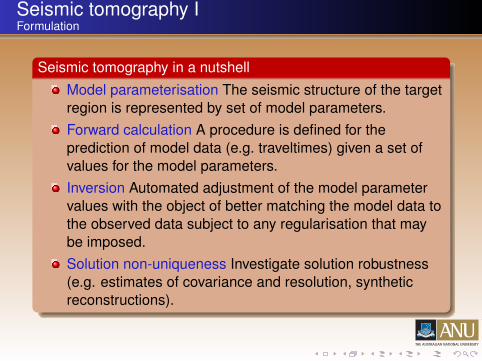
Model parameterisation The seismic structure of the targetregion is represented by set of model parameters.Forward calculation A procedure is defined for theprediction of model data (e.g. traveltimes) given a set ofvalues for the model parameters.Inversion Automated adjustment of the model parametervalues with the object of better matching the model data tothe observed data subject to any regularisation that maybe imposed.Solution non-uniqueness Investigate solution robustness(e.g. estimates of covariance and resolution, syntheticreconstructions).

Seismic tomography IModel parameterisation

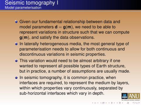
Given our fundamental relationship between data andmodel parameters d = g(m), we need to be able torepresent variations in structure such that we can computeg(m), and satisfy the data observations.In laterally heterogeneous media, the most general type ofparameterisation needs to allow for both continuous anddiscontinuous variations in seismic properties.This variation would need to be almost arbitrary if onewanted to represent all possible types of Earth structure,but in practice, a number of assumptions are usually made.In seismic tomography, it is common practice, wheninterfaces are required, to represent the medium by layers,within which properties vary continuously, separated bysub-horizontal interfaces which vary in depth.


Schematic illustration of a layered parameterisation.

( )x,zv 4

( )x,zv 1

( )x,zv 2

( )x,zv 3

z

x


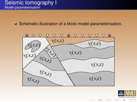
The relative simplicity of this representation makes itamenable to fast and robust data prediction, and alsoallows a variety of later arriving phases to be computedHowever, in exploration seismology, where data coverageis usually dense, and near surface complexities(particularly faults) often need to be accuratelyrepresented, this class of parameterisation can be toorestrictive.An alternative approach is to divide the model region upinto an aggregate of irregularly shaped volume elementswithin which material property varies smoothly, but isdiscontinuous across element boundariesHowever, in the presence of such complexity, the dataprediction problem and inverse problem are much moredifficult to solve.


Schematic illustration of a block-model parameterisation.

( )x,zv 11

( )x,zv ( )x,zv

( )x,z

v 6

( )x,zv

x,zv

( )x,zv 4

( )x,zv 5( )x,z

v 9

( )x,zv 8

( )x,zv 7

10( )

2

3

1


Common parameterisations used to describe wave speedvariations (or other seismic properties) in a continuuminclude constant velocity (or slowness) blocks,triangular/tetrahedral meshes within which velocity isconstant or constant in gradient, and grids of velocitynodes which are interpolated using a predefined function.Constant velocity blocks are conceptually simple, butrequire a fine discretisation in order to subdue theundesirable artifact of block boundaries.These discontinuities also have the potential tounrealisticly distort the wavefield and make the two-pointray tracing problem more unstable.


Triangular/tetrahedral meshes are flexible and allowanalytic ray tracing when velocity is constant or constant ingradient within a cell.However, like constant velocity blocks, they usually requirea fine discretisation, and can also destabilise the dataprediction problem.Velocity grids which describe a continuum using aninterpolant offer the possibility of smooth variations withrelatively few parameters, but are generally morecomputationally intensive to evaluate.


One of the simplest and most popular interpolants ispseudo-linear interpolation, which in 3-D Cartesiancoordinates is:

v(x , y , z) =2∑

i=1

2∑j=1

2∑k=1

V (xi , yj , zk )

(1−

∣∣∣∣ x − xi

x2 − x1

∣∣∣∣)×

(1−

∣∣∣∣ y − yj

y2 − y1

∣∣∣∣) (1−

∣∣∣∣ z − zk

z2 − z1

∣∣∣∣)where V (xi , yj , zk ) are the velocity (or some other seismicproperty) values at eight grid points surrounding (x , y , z).In the above equation v is continuous, but its gradient ∇vis not (i.e. C0 continuity). Despite this limitation, pseudolinear interpolation between nodes is a popular choice inseismic tomography.


Higher order interpolation functions are required if thevelocity field is to have continuous first and secondderivatives, which is usually desirable for schemes whichnumerically solve the ray tracing or eikonal equations.There are many types of spline functions that can be usedfor interpolation, including Cardinal, B-splines and splinesunder tension.Cubic B-splines are particularly useful, as they offer C2

continuity, local control and the potential for an irregulardistribution of nodes.


For a set of velocity values Vi,j,k on a 3-D grid of pointspi,j,k = (xi,j,k , yi,j,k , zi,j,k ), the B-spline for the ijk th volumeelement is

BBBi,j,k (u, v , w) =2∑

l=−1

2∑m=−1

2∑n=−1

bl(u)bm(v)bn(w)qi+l,j+m,k+n,

where qi,j,k = (Vi,j,k , pi,j,k ). Thus, the three independentvariables 0 ≤ u, v , w ≤ 1 define the velocity distribution ineach volume element.The weighting factors bi are the uniform cubic B-splinefunctions.


Rather than use velocity grids in the spatial domain todescribe smooth media, one could also exploit thewavenumber domain by employing a spectralparameterisation.These are often popular for global applications e.g.spherical harmonics, but can also be used for problems ona local or regional scale.One approach (in 2-D) is to use a truncated Fourier seriesexpressed as:

s(r) = a00 +N∑

m=1

[am0 cos(k · r) + bm0 sin(k · r)]

+N∑

m=−N

N∑n=1

[amn cos(k · r) + bmn sin(k · r)],


In the above equation, r = x i + zj and k = mπk0i + nπk0jare the position and wavenumber vector respectively, andamn and bmn are the amplitude coefficients of the (m, n)th

harmonic term.Although the above equation is infinitely differentiable, it isglobally supported in that adjustment of any amplitudecoefficient influences the entire model.Spectral parameterisations have been used in a number oftomographic studies, particularly those involving globaldatasets.


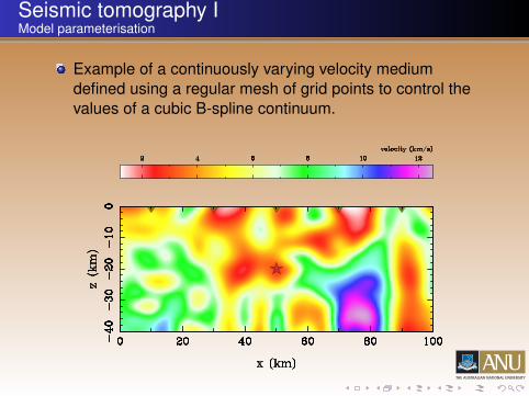
Example of a continuously varying velocity mediumdefined using a regular mesh of grid points to control thevalues of a cubic B-spline continuum.


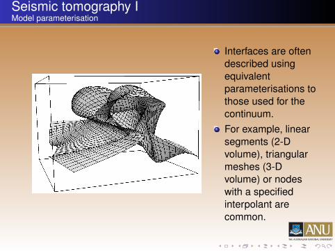
Interfaces are oftendescribed usingequivalentparameterisations tothose used for thecontinuum.For example, linearsegments (2-Dvolume), triangularmeshes (3-Dvolume) or nodeswith a specifiedinterpolant arecommon.


Finally, it is worth noting that irregular parameterisationsare occasionally used.For many large seismic datasets, path distribution can behighly heterogeneous, resulting in a spatial variability inresolving powerThe ability to “tune" a parameterisation to these variationsusing some form of irregular mesh has a range of potentialbenefits, including increased computational efficiency(fewer unknowns), improved stability of the inverseproblem, and improved extraction of structural informationCompletely unstructured meshes, such as those that useDelaunay tetrahedra or Voronoi polyhedra, offer high levelsof adaptability, but have special book-keeping requirementswhen solving the forward problem of data prediction.

Seismic tomography IForward calculation

The forward problem in seismic tomography requires thecalculation of model data, given a set of values for themodel parameters.In the case of traveltime tomography, the aim is to computesource-receiver traveltimes for a given velocity model.For surface wave tomography, on the other hand, the aimis usually to try and compute a long period syntheticwaveform.In the majority of cases, some form of ray tracing orwavefront tracking is used. These techniques werediscussed in detail in Lecture 8.

Seismic tomography IForward calculation

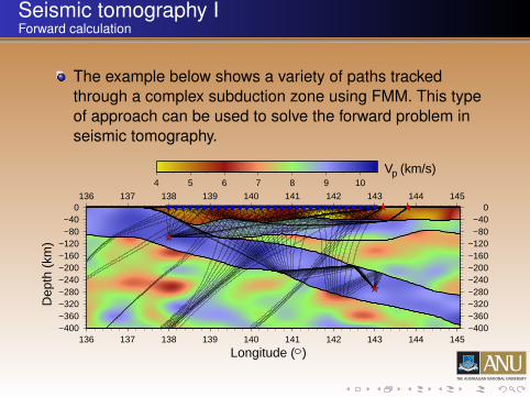
The example below shows a variety of paths trackedthrough a complex subduction zone using FMM. This typeof approach can be used to solve the forward problem inseismic tomography.

−400−360−320−280−240−200−160−120

−80−40

0

−400−360−320−280−240−200−160−120

−80−40

0

136 137 138 139 140 141 142 143 144 145

136 137 138 139 140 141 142 143 144 145

4 5 6 7 8 9 10

Dep

th (

km)

pV (km/s)

Longitude ( )

Seismic tomography IInversion

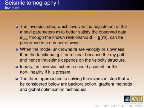
The inversion step, which involves the adjustment of themodel parameters m to better satisfy the observed datadobs through the known relationship d = g(m), can beperformed in a number of ways.When the model unknowns m are velocity or slowness,then the functional g is non-linear because the ray pathand hence traveltime depends on the velocity structure.Ideally, an inversion scheme should account for thisnon-linearity if it is present.The three approaches to solving the inversion step that willbe considered below are backprojection, gradient methodsand global optimisation techniques.

Seismic tomography IBackprojection

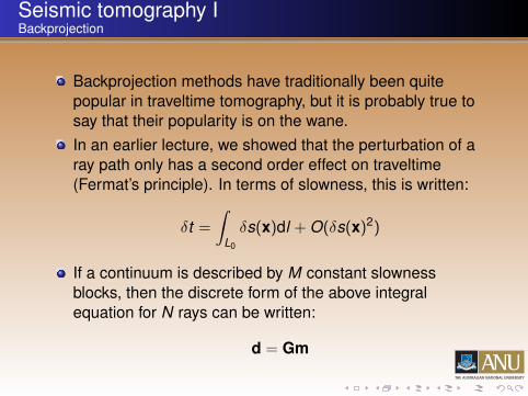
Backprojection methods have traditionally been quitepopular in traveltime tomography, but it is probably true tosay that their popularity is on the wane.In an earlier lecture, we showed that the perturbation of aray path only has a second order effect on traveltime(Fermat’s principle). In terms of slowness, this is written:

δt =

∫L0

δs(x)dl + O(δs(x)2)

If a continuum is described by M constant slownessblocks, then the discrete form of the above integralequation for N rays can be written:

d = Gm


In the above equation, d are the traveltime residuals, m theslowness perturbations and G an N ×M matrix of raylengths lij corresponding to the distance traversed by eachray in each block.Note that for the general case m (e.g. velocity nodes,interface depths etc.) G = ∂g/∂m where g(m) is themodel prediction.Many of the elements of G will be zero since each ray pathwill usually only traverse a small subset of the M blocks.Backprojection methods can be used to solve d = Gm forthe slowness perturbations m by iteratively mappingtraveltime anomalies into slowness perturbations along theray paths until the data are satisfied.


Two well known backprojection techniques for solvingd = Gm are the Algebraic Reconstruction Technique (ART)and the Simultaneous Iterative Reconstruction Technique(SIRT), both of which originate from medical imaging.In ART, the model is updated on a ray by ray basis. Theresidual dn for the nth ray path is distributed along the pathby adjusting each component of m in proportion to thelength lnj of the ray segment in the j th cell:

mk+1j = mk

j +tk+1n lnjM∑

m=1l2nm

In the above equation, tk+1n = dn − tk

n is the differencebetween the residuals at the 0th and k th iteration, mk

j is theapproximation to the j th model parameter at the k th

iteration, m1j = 0 and t1

n = 0.


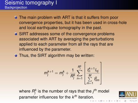
The main problem with ART is that it suffers from poorconvergence properties, but it has been used in cross-holeand local earthquake tomography in the past.SIRT addresses some of the convergence problemsassociated with ART by averaging the perturbationsapplied to each parameter from all the rays that areinfluenced by the parameter.Thus, the SIRT algorithm may be written:

mk+1j = mk

j +1

Rkj

Rkj∑

n=1

tk+1n lnjM∑

m=1l2nm

where Rk

j is the number of rays that the j th modelparameter influences for the k th iteration.


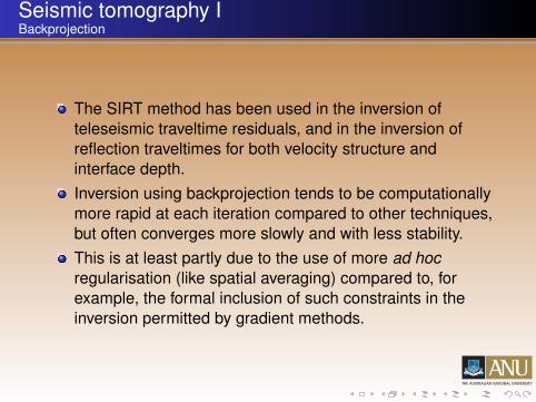
The SIRT method has been used in the inversion ofteleseismic traveltime residuals, and in the inversion ofreflection traveltimes for both velocity structure andinterface depth.Inversion using backprojection tends to be computationallymore rapid at each iteration compared to other techniques,but often converges more slowly and with less stability.This is at least partly due to the use of more ad hocregularisation (like spatial averaging) compared to, forexample, the formal inclusion of such constraints in theinversion permitted by gradient methods.

Seismic tomography IGradient methods

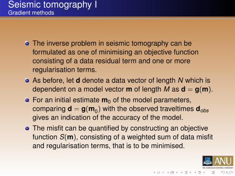
The inverse problem in seismic tomography can beformulated as one of minimising an objective functionconsisting of a data residual term and one or moreregularisation terms.As before, let d denote a data vector of length N which isdependent on a model vector m of length M as d = g(m).For an initial estimate m0 of the model parameters,comparing d = g(m0) with the observed traveltimes dobsgives an indication of the accuracy of the model.The misfit can be quantified by constructing an objectivefunction S(m), consisting of a weighted sum of data misfitand regularisation terms, that is to be minimised.


An essential component of the objective function is a termΨ(m) which measures the difference between theobserved and predicted data.If it is assumed that the error in the relationshipdobs ≈ g(mtrue) is Gaussian, then a least squares or L2measure of this difference is suitable:

Ψ(m) = ‖g(m)− dobs‖2

If uncertainty estimates have been made for the observeddata (usually based on picking error), then more accuratedata are given a greater weight in the objective function bywriting Ψ(m) as:

Ψ(m) = (g(m)− dobs)T C−1

d (g(m)− dobs)

where Cd is a data covariance matrix.


If the errors are assumed to be uncorrelated, thenCd = [δij(σ

jd)2] where σj

d is the uncertainty of the j th datapoint.A common problem with tomographic inversion is that notall model parameters will be well constrained by the dataalone (i.e. the problem may be under-determined ormixed-determined).A regularisation term Φ(m) is often included in theobjective function to provide additional constraints on themodel parameters, thereby reducing the non-uniquenessof the solution.The regularisation term is typically defined as:

Φ(m) = (m−m0)T C−1

m (m−m0)

where Cm is an a priori model covariance matrix.


If uncertainties in the initial model are assumed to beuncorrelated, then Cm = [δij(σ

jm)2] where σj

m is theuncertainty associated with the j th model parameter of theinitial model.The effect of Φ(m) is to encourage solution models m thatare near a reference model m0. The values used in Cm areusually based on prior information.Another approach to regularisation is the minimumstructure solution which attempts to find an acceptabletrade-off between satisfying the data and finding a modelwith the minimum amount of structural variation.One way of including this requirement in the objectivefunction is to use the term:

Ω(m) = mT DT Dm

where Dm is a finite difference estimate of a specifiedspatial derivative.


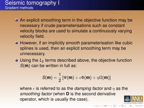
An explicit smoothing term in the objective function may benecessary if crude parameterisations such as constantvelocity blocks are used to simulate a continuously varyingvelocity field.However, if an implicitly smooth parameterisation like cubicsplines is used, then an explicit smoothing term may beunnecessary.Using the L2 terms described above, the objective functionS(m) can be written in full as:

S(m) =12

[Ψ(m) + εΦ(m) + ηΩ(m)]

where ε is referred to as the damping factor and η as thesmoothing factor (when D is the second derivativeoperator, which is usually the case).


ε and η govern the trade-off between how well the solutionmest will satisfy the data, how closely mest is to m0, andthe smoothness of mest .

Model perturbation

ηη

η(b)

smalloptimum

large

small large

low

high

Dat

a fi

t

Model roughness

(a)

small

Dat

a fi

thi

ghlo

w

largesmall

ε

εε

large

optimum


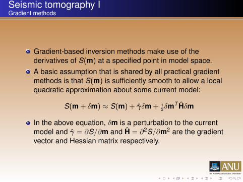
Gradient-based inversion methods make use of thederivatives of S(m) at a specified point in model space.A basic assumption that is shared by all practical gradientmethods is that S(m) is sufficiently smooth to allow a localquadratic approximation about some current model:

S(m + δm) ≈ S(m) + γδm + 12δmT Hδm

In the above equation, δm is a perturbation to the currentmodel and γ = ∂S/∂m and H = ∂2S/∂m2 are the gradientvector and Hessian matrix respectively.


For our chosen form of objective function,

γ = GT C−1d [g(m)− dobs] + εC−1

m (m−m0) + ηDT Dm

H = GT C−1d G +∇mGT C−1

d [g(m)− dobs] + εC−1m + ηDT D

where G = ∂g/∂m is the Fréchet matrix of partialderivatives calculated during the solution of the forwardproblem.Since g is generally non-linear, the minimisation of S(m)requires an iterative approach:

mn+1 = mn + δmn

where m0 is the initial model.


The objective function is minimised for the current ray pathestimate at each step to produce mn+1, after which newray paths are computed for the next iteration.The iterations cease either when the observed traveltimesare satisfied or when the change in S(m) with iterationgets sufficiently small.One approach to estimating δmn is the Gauss-Newtonmethod. It locates the minimum of the tangent paraboloidto S(m) at mn.At the minimum of S, the gradient will vanish, so m isrequired such that:

F(m) = GT C−1d (g(m)−dobs)+εC−1

m (m−m0)+ηDT Dm = 0

where F(m) = γ.


If we are at some point mn, then a more accurate estimatemn+1 can be obtained using a Taylor series expansion:

Fi(m1n+1, . . . , mM

n+1) = Fi(m1n, . . . , mM

n )

+M∑

j=1

(mjn+1 −mj

n)∂Fi

∂mj

∣∣∣∣mn

= 0

This may be rewritten as

mn+1 = mn −[

∂F∂m

]−1

n[Fn] = mn −

[∂2S∂m2

]−1

n

[∂S∂m

]n

where (∂S/∂m)n is the gradient vector and (∂2S/∂m2)n isthe Hessian matrix.


Substitution of the expressions given earlier for (∂S/∂m)nand (∂2S/∂m2)n yields the Gauss-Newton solution:

δmn = −[GTn C−1

d Gn +∇mGTn C−1

d (g(mn)− dobs) + εC−1m + ηDT D]−1

×[GTn C−1

d [g(mn)− dobs] + εC−1m (mn −m0) + ηDT Dmn]

If instead we assume that the relationship d = g(m) islinearisable then

dobs ≈ g(m0) + G(m−m0)

or δd = Gδm with δd = dobs − g(m0) and δm = m−m0.


Because a one-step solution is possible in the linear case,the objective function is sometimes written:

S(m) =12

[(Gδm− δd)T C−1

d (Gδm− δd)

+εδmT C−1m δm + ηδmT DT Dδm

]where last term on the RHS smooths the perturbations tothe prior model.The functional in this case is:

F(m) = GT C−1d (Gδm− δd) + εC−1

m δm + ηDT Dδm = 0


The solution can therefore be written as:

δm = [GT C−1d G + εC−1

m + ηDT D]−1GT C−1d δd

When no smoothing is used (η = 0), then:

δm = [GT C−1d G + C−1

m ]−1GT C−1d δd

which is the maximum likelihood solution to the inverseproblem or the stochastic inverse.The above two expressions are sometimes referred to asthe Damped Least Squares (DLS) solutions to the inverseproblem (particularly when η = 0).


Solutions to the above equations can be obtained usingstandard methods for solving large linear systems ofequations.Techniques such as LU decomposition or SVD can beused to solve small to moderate sized problems.For large problems, conjugate gradients and LSQR aremore appropriate, particular for sparse matrices.Methods for minimisation of the objective function thatdon’t require the solution of a large linear system ofequations include steepest descent, conjugate gradientand subspace methods.

Seismic tomography IFully non-linear inversion

The inversion methods described above are local in thatthey exploit information in regions of model space near aninitial model estimate and thus avoid an extensive searchof model space.Consequently, they cannot guarantee convergence to aglobal minimum solution. Local methods are prone toentrapment in local minima, especially if the subsurfacevelocity structure is complex and the starting model is notclose to the true model.In many realistic applications, particularly at regional andglobal scales, the need for global optimisation techniquesis hard to justify, because the a priori model information isrelatively accurate and lateral heterogeneities are not verylarge


However, the crust and lithosphere are generally less wellconstrained by a priori information and are also much moreheterogeneous. This means that the initial model is likelyto be more distant from the global minimum solution, andentrapment in a local minimum becomes more of aconcern.Two non-linear schemes that have been used in seismictomography are genetic algorithms and simulatedannealing.Genetic algorithms use an analogue to biological evolutionto develop new models from an initial pool of randomlypicked models.Simulated annealing is based on an analogy with physicalannealing in thermodynamic systems to guide variations tothe model parameters.


Global optimisation using stochastic methods is a rapidlydeveloping field of science. However, current applicationsto seismic tomography problems have been limited due tocomputational expense.Hybrid approaches are sometimes implemented, whichinvolve using a non-linear technique to find the globalminimum solution of a coarse model (i.e. few modelparameters). Iterative non-linear schemes are then appliedto refine the solution.Simulated annealing has been used in the inversion ofreflection traveltimes for 2-D velocity structure andinterface geometry.Genetic algorithms have been used in the inversion ofrefraction traveltimes for 2-D velocity structure.

Seismic tomography ISolution non-uniqueness

The process of producing a solution to an inverse problemusing the above methods is not complete until someestimate of solution robustness or quality is made.Simply producing a single solution that minimises anobjective function (i.e. best satisfies the data and a prioriconstraints) without knowledge of resolution ornon-uniqueness is inadequate.In seismic tomography, one common approach toassessing solution robustness is to apply syntheticresolution tests.Alternatively, if the assumption of local linearity isjustifiable, formal estimates of model covariance andresolution can be made.


Parameterisations that describe continuous variations inseismic properties often opt for resolution tests thatattempt to reconstruct a synthetic model using the samesource-receiver geometry as the real experiment.The rationale behind this approach is that if a knownstructure with similar length scales to the solution modelcan be recovered using the same (for linearised solutions)or similar (for iterative non-linear solutions) ray paths, thenthe solution model should be reliableThe quality criterion is the similarity between the recoveredmodel and the synthetic model.The so-called “checkerboard test", in which the syntheticmodel is divided into alternating regions of high and lowvelocity with a length scale equal (or greater) to thesmallest wavelength structure recovered in thesolution model, is a common test model.


velo

city

per

turb

atio

n

0

-

+

dept

h

horizontal distance


For an objective function with no smoothing term, theresolution matrix can be written:

R = I− CMC−1m

The corresponding a posteriori covariance matrix can bewritten

CM = ε[GT C−1d G + εC−1

m ]−1

These quantities are derived from linear theory. Thediagonal elements of CM indicate the posterior uncertaintyassociated with each model parameter.The diagonal elements of R range between zero and 1; intheory, when R = I, the model is perfectly resolved.

peat8002 - seismology lecture 16: seismic tomography...

Documents