The 2006 Federated Logic Conference

The Seattle Sheraton Hotel and Towers

Seattle, Washington

August 10 - 22, 2006

ICLP’06 Workshop

PDPAR’06:Pragmatical Aspects of Decision Procedures

in Automated Reasoning

August 21st, 2006

Proceedings

Editors:

Byron Cook, Roberto Sebastiani

Table of Contents

Table of Contents . . . . . . . . . . . . . . . . . . . . . . . . . . . . . . . . . . . . . . . . . . . . . . . . . . . . . . . . iii

Program Committee . . . . . . . . . . . . . . . . . . . . . . . . . . . . . . . . . . . . . . . . . . . . . . . . . . . . . . iv

Additional Reviewers . . . . . . . . . . . . . . . . . . . . . . . . . . . . . . . . . . . . . . . . . . . . . . . . . . . . . iv

Foreword . . . . . . . . . . . . . . . . . . . . . . . . . . . . . . . . . . . . . . . . . . . . . . . . . . . . . . . . . . . . . . . . . v

Keynote contributions (abstracts)

Proof Procedures for Separated Heap Abstractions

Peter O’Hearn . . . . . . . . . . . . . . . . . . . . . . . . . . . . . . . . . . . . . . . . . . . . . . . . . . . . . . . . . . . . 1

The Power of Finite Model Finding

Koen Claessen . . . . . . . . . . . . . . . . . . . . . . . . . . . . . . . . . . . . . . . . . . . . . . . . . . . . . . . . . . . . 2

Original papers

Mothers of Pipelines

Krstic, Jones, O’Leary . . . . . . . . . . . . . . . . . . . . . . . . . . . . . . . . . . . . . . . . . . . . . . . . . . . . . 3

Applications of hierarchical reasoning in the verification of complex systems

Jacobs, Sofronie-Stokkermans . . . . . . . . . . . . . . . . . . . . . . . . . . . . . . . . . . . . . . . . . . . . . 15

Towards Automatic Proofs of Inequalities Involving Elementary Functions

Akbarpour, Paulson . . . . . . . . . . . . . . . . . . . . . . . . . . . . . . . . . . . . . . . . . . . . . . . . . . . . . . 27

Rewrite-Based Satisfiability Procedures for Recursive Data Structures

Bonacina, Echenim . . . . . . . . . . . . . . . . . . . . . . . . . . . . . . . . . . . . . . . . . . . . . . . . . . . . . . 38

An Abstract Decision Procedure for Satisfiability in the Theory of Recursive Data

Types

Barrett, Shikanian, Tinelli . . . . . . . . . . . . . . . . . . . . . . . . . . . . . . . . . . . . . . . . . . . . . . . . .50

Presentation-only papers (abstracts)

A Framework for Decision Procedures in Program Verification

Strichman, Kroening . . . . . . . . . . . . . . . . . . . . . . . . . . . . . . . . . . . . . . . . . . . . . . . . . . . . . 62

Easy Parameterized Verification of Biphase Mark and 8N1 Protocols

Brown, Pike . . . . . . . . . . . . . . . . . . . . . . . . . . . . . . . . . . . . . . . . . . . . . . . . . . . . . . . . . . . . . 63

Predicate Learning and Selective Theory Deduction for Solving Difference Logic

Wang, Gupta, Ganai . . . . . . . . . . . . . . . . . . . . . . . . . . . . . . . . . . . . . . . . . . . . . . . . . . . . . .64

Deciding Extensions of the Theory of Arrays by Integrating Decision Procedures

and Instantiation Strategies

Ghilardi, Niccolini, Ranise, Zucchelli . . . . . . . . . . . . . . . . . . . . . . . . . . . . . . . . . . . . . . 65

Producing Conflict Sets for Combinations of Theories

Ranise, Ringeissen, Tran . . . . . . . . . . . . . . . . . . . . . . . . . . . . . . . . . . . . . . . . . . . . . . . . . . 66

iii

Program Committee

Byron Cook (Microsoft Research, UK) [co-chair]

Roberto Sebastiani (Universita di Trento, Italy) [co-chair]

Alessandro Armando (Universita di Genova)

Clark Barrett (New York University)

Alessandro Cimatti (ITC-Irst, Trento)

Leonardo de Moura (SRI International)

Niklas Een (Cadence Design Systems)

Daniel Kroening (ETH-Zurich)

Shuvendu Lahiri (Microsoft Research)

Robert Nieuwenhuis (Technical University of Catalonia)

Silvio Ranise (LORIA, Nancy)

Eli Singerman (Intel Corporation)

Ofer Strichman (Technion)

Aaron Stump (Washington University)

Cesare Tinelli (University of Iowa)

Ashish Tiwari (Stanford Research Institute, SRI)

Additional reviewers

Nicolas Blanc

Juergen Giesl

Guillem Godoy

Kalyanasundaram Krishnamani

Michal Moskal

Enrica Nicolini

Albert Oliveras

Zvonimir Rakamaric

Simone Semprini

Armando Tacchella

Francesco Tapparo

Christoph Wintersteiger

Daniele Zucchelli

iv

Foreword

This volume contains the proceedings of the 4th Workshop on Pragmatics of

Decision Procedures in Automated Reasoning (PDPAR’06), held in Seattle, USA,

on August 21st, 2006, as part of the 2006 Federated Logic Conference (FLoC’06)

and affiliated with the 3rd International Joint Conference on Automated Reasoning

(IJCAR’06).

The applicative importance of decision procedures for the validity or the satisfi-

ability problem in decidable first-order theories is being increasingly acknowledged

in the verification community: many interesting and powerful decision procedures

have been developed, and applied to the verification of word-level circuits, hybrid

systems, pipelined microprocessors, and software.

The PDPAR’06 workshop has brought together researchers interested in both

the theoretical and the pragmatical aspects of decision procedures, giving them a

forum for presenting and discussing not only theoretical and algorithmic issues, but

also implementation and evaluation techniques, with the ultimate goal of making

new decision procedures possible and old decision procedures more powerful and

more useful.

In this edition of PDPAR we have allowed not only original papers, but also

“presentation-only papers”, i.e., papers describing work previously published in

non-FLOC’06 forums (which are not inserted in the proceedings). We are allow-

ing the submission of previously published work in order to allow researchers to

communicate good ideas that the PDPAR attendees are potentially unaware of.

The program included:

• two keynote presentations by Peter O’Hearn, University of London, and Koen

Claessen, Chalmers University.

• 10 technical paper presentations, including 5 original papers and 5 “presentation-

only” papers.

• A discussion session.

Additional details for PDPAR’06 (including the program) are available at the

web site http://www.dit.unitn.it/˜rseba/pdpar06/.

We gratefully acknowledge the financial support of Microsoft Research.

Seattle, August 2006

Byron Cook Microsoft Research, Cambridge, UK

Roberto Sebastiani DIT, University of Trento, Italy

v

vi

Proof Procedures for

Separated Heap Abstractions(keynote presentation)

Peter O’Hearn

Queen Mary, University of London

ohearn@dcs.qmul.ac.uk

Abstract

Separation logic is a program logic geared towards reasoning aboutprograms that mutate heap-allocated data structures. This talk de-scribes ideas arising from joint work with Josh Berdine and CristianoCalcagno on proof procedure for a sublogic of separation logic that isoriented to lightweight program verification and analysis. The prooftheory uses ideas from substructural logic together with induction-freereasoning about inductive definitions of heap structures. Substructuralreasoning is used to to infer frame axioms, which describe the portionof a heap that is not altered by a procedure, as well as to discharge ver-ification conditions; more precisely, the leaves of failed proofs can giveus candidate frame axioms. Full automation is achieved through theuse of special axioms that capture properties that would normally beproven using by induction. I will illustrate the proof method throughits use in the Smallfoot static assertion checker, where it is used toprove verification conditions and infer frame axioms, as well as in theSpace Invader program analysis, where it is used to accelerate the con-vergence of fixed-point calculations.

1

The Power of Finite Model Finding(keynote presentation)

Koen Claessen

Chalmers University of Technology and

Jasper Design Automation

koen@cs.chalmers.se

Abstract

Paradox is a tool that automatically finds finite models for first-order logic formulas, using incremental SAT. In this talk, I will presenta new look on the problem of finding finite models for first-order logicformulas. In particular, I will present a novel application of finite modelfinding to the verification of finite and infinite state systems; here,a finite model finder can be used to automatically find abstractionsof systems for use in safety property verification. In this verificationprocess, it turns out to be vital to use typed (or sorted) first-orderformulas. Finding models for typed formulas brings the freedom touse different domain sizes for each type. How to choose these differentdomain sizes is still very much an unexplored problem. We show howa simple extension to a SAT-solver can be used to guide the search fortyped models with several domains of different sizes.

2

Mothers of Pipelines

Sava Krstic, Robert B. Jones, and John W. O’Leary

Strategic CAD Labs, Intel Corporation, Hillsboro, OR, USA

Abstract. We present a novel method for pipeline verification using SMT solvers.It is based on a non-deterministic “mother pipeline” machine (MOP) that abstractsthe instruction set architecture (ISA). The MOP vs. ISA correctness theorem splitsnaturally into a large number of simple subgoals. This theorem reduces proving thecorrectness of a given pipelined implementation of the ISA to verifying that each ofits transitions can be modeled as a sequence of MOP state transitions.

1 Introduction

Proving correctness of microarchitectural processor designs (MA) with respect totheir instruction set architecture (ISA) amounts to establishing a simulation relationbetween the behaviors of MA and ISA. There are different ways in the literature toformulate the correctness theorem that relates the steps of the two machines [1], butthe complexity of the MA’s step function remains the major impediment to practicalverification. The challenge is to find a systematic way to break the verification effortinto manageable pieces.

We propose a solution based on the obvious fact that the execution of anyinstruction can be seen as a sequence of smaller actions (let us call them mini-steps inthis informal overview), and the observation that the mini-steps can be understoodat an abstract level, without mentioning any concrete MA. Examples of mini-stepsare fetching an instruction, getting an operand from the register file, having anoperand forwarded by a previous instruction in the pipeline, writing a result to theregister file, and retiring. We introduce an intermediate specification MOP betweenISA and MA that describes the execution of each instruction as a sequence of mini-steps. By design, our highly non-deterministic intermediate specification admits abroad range of implementations. For example, MOP admits implementations thatare out-of-order or not, speculative or not, superscalar or not, etc. This approachallows us to separate the implementation-independent proof obligations that relateISA to MOP from those that rely upon the details of the MA. This can potentiallyamortize some of the proof effort over several different designs.

The concept of parcels, formalizing partially-executed instructions, will be neededfor a thorough treatment of mini-steps. We will follow the intuition that from anygiven state of any MA one can always extract the current state of its ISA componentsand infer a queue of parcels currently present in the MA pipeline. In Section 2, wegive a precise definition of a transition system MOP whose states are pairs of theform 〈ISA state, queue of parcels〉, and whose transitions are mini-steps as describedabove. Intuitively, it is clear that with a sufficiently complete set of mini-steps we will

be able to model any MA step in this transition system as a sequence of mini-steps.Similarly, it should be possible to express any ISA step as a sequence of mini-stepsof MOP .

Figure 1 indicates that correctness of a microarchitecture MA with respect toISA is implied by correctness results that relate these machines with MOP . InSection 3, we will prove the crucial MOP vs. ISA correctness property: despite itsnon-determinism, all MOP executions correspond to ISA executions. The proof restson the local confluence of MOP . (Proofs are provided in the Appendix.)

MA1

++WWWWWW

... MOP oo //______ ISA

MAn

33gggggg

Fig. 1. With transitions that express atomic steps in instruction execution, a mother of pipelinesMOP simulates the ISA and its multiple microarchitectural implementations. Simulation a laBurch-Dill flushing justifies the arrow from MOP to ISA.

The MA vs. MOP relationship is discussed in Section 4. We will see that all oneneeds to prove here is a precise form of the simulation mentioned above: there existsan abstraction function that maps MA states to MOP states such that for any twostates joined by a MA transition, the corresponding MOP states are joined by asequence of mini-steps.

MA vs. MOP vs. ISA correctness theorems systematically reduce to numeroussubgoals, suitable for automated SMT solvers (“satisfiability modulo theories”). Weused CVC Lite [4] and our initial experience is discussed in Section 5.

2 MOP Definition

The MOP definition depends on the ISA and the class of pipelined implementationsthat we are interested in. The particular MOP described in this section has a simpleload-store ISA and can model complex superscalar implementations with out-of-order execution and speculation.

2.1 The Instruction Set Architecture

ISA is a deterministic transition system with system variables pc : IAddr, rf : RF,mem : MEM, imem : IMEM. We assume the types Reg and Word of registers andmachine words, so that rf can be viewed as a Reg-indexed array with Word values.Similarly, mem can be viewed as a Word-indexed array with values in Word, while

4

instruction imem.pc actions

opc1 dest src1 src2 pc := pc + 4 rf .dest := alu opc1 (rf .src1 ) (rf .src2 )

opc2 dest src1 imm pc := pc + 4 rf .dest := alu opc2 (rf .src1 ) imm

ld dest src1 offset pc := pc + 4 rf .dest := mem.(rf .src1 + offset)

st src1 dest offset pc := pc + 4 mem.(rf .dest + offset) := rf .src1

opc3 reg offset pc :=

target if takenpc + 4 otherwise

, where

target = get target pc offsettaken = get taken (get test opc3 ) (rf .reg)

Fig. 2. ISA instruction classes (left column) and corresponding transitions. The variablesdest , src1 , src2 , reg have type Reg, and imm, offset have type Word. For the three opcodes, wehave opc1 ∈ add, sub,mult, opc2 ∈ addi, subi,multi, opc3 ∈ beqz, bnez, j.

imem is an IAddr-indexed array with values in the type Instr of instructions. Instruc-tions fall into five classes that are identified by the predicates alu reg , alu imm, ld ,st , branch. The form of an instruction of each class is given in Figure 2. The figurealso shows the ISA transitions—the change-of-state equations defined separately foreach instruction class.

2.2 State

Parcels are records with the following fields:

instr : Instr⊥ my pc : IAddr⊥ dest , src1 , src2 : Reg⊥imm : Word⊥AA opc : Opcode⊥ data1 , data2 , res,mem addr : Word⊥tkn : bool⊥ next pc : IAddr⊥AA wb : ⊥,> pc upd : ⊥, , ,>

The subscript ⊥ to a type indicates the addition of the element ⊥ (“undefined”) tothe type. The empty parcel has all fields equal to ⊥. The field wb indicates whetherthe parcel has written back to the register file (for arithmetical parcels and loads)or to the memory (for stores). Similiarly, pc upd indicates whether the parcel hascaused the update of pc. The additional values and are to record that the parcelhas updated pc speculatively and that it mispredicted.

In addition to the architected state components pc, rf , mem, imem, the stateof MOP contains integers head and tail , and a queue of parcels q . The queue isrepresented by an integer-indexed array with head and tail defining its front andback ends. We write idx j as an abbreviation for the predicate head ≤ j ≤ tail ,saying that j is a valid index in q. The jth parcel in q will be denoted q.j.

2.3 Transitions

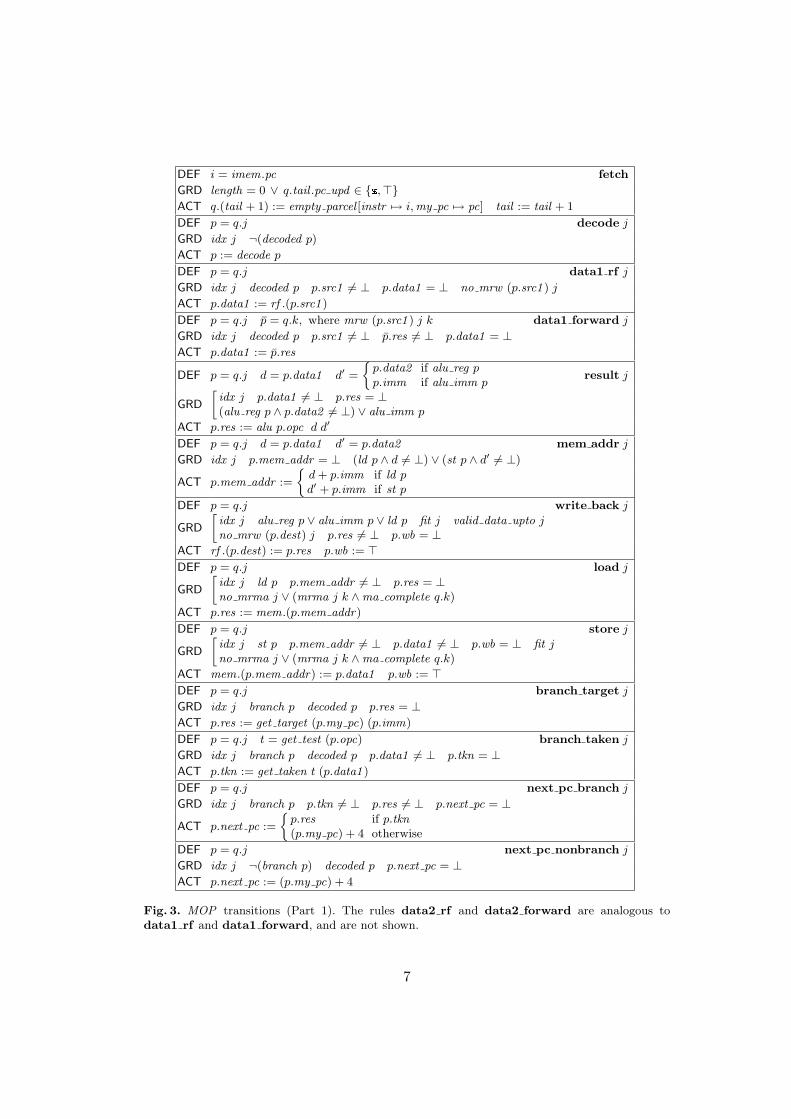
The transitions of MOP are defined by the rules given in Figures 3 and 4. Each ruleis a guarded parallel assignment described in the def/grd/act format, where defcontains local definitions, grd (guard) is the set of predicates defining the rule’s

5

domain, and act are the assignments made when the rule fires. Some rules containadditional predicates and functions, defined next.

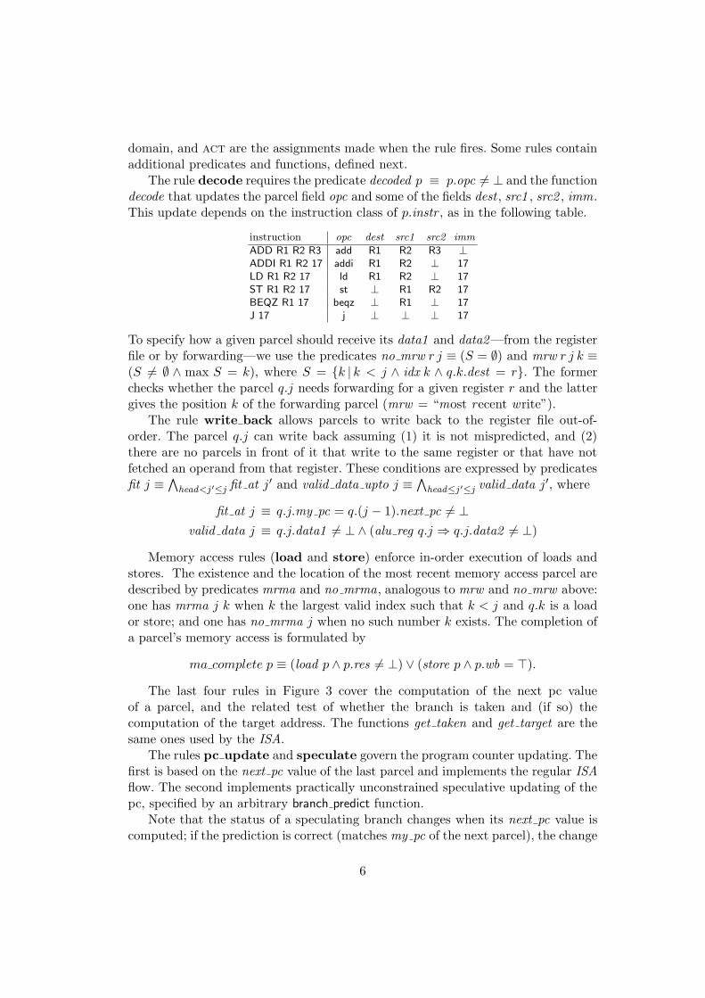
The rule decode requires the predicate decoded p ≡ p.opc 6= ⊥ and the functiondecode that updates the parcel field opc and some of the fields dest , src1 , src2 , imm.This update depends on the instruction class of p.instr , as in the following table.

instruction opc dest src1 src2 imm

ADD R1 R2 R3 add R1 R2 R3 ⊥ADDI R1 R2 17 addi R1 R2 ⊥ 17

LD R1 R2 17 ld R1 R2 ⊥ 17

ST R1 R2 17 st ⊥ R1 R2 17

BEQZ R1 17 beqz ⊥ R1 ⊥ 17

J 17 j ⊥ ⊥ ⊥ 17

To specify how a given parcel should receive its data1 and data2 —from the registerfile or by forwarding—we use the predicates no mrw r j ≡ (S = ∅) and mrw r j k ≡(S 6= ∅ ∧ max S = k), where S = k | k < j ∧ idx k ∧ q.k.dest = r. The formerchecks whether the parcel q.j needs forwarding for a given register r and the lattergives the position k of the forwarding parcel (mrw = “most recent write”).

The rule write back allows parcels to write back to the register file out-of-order. The parcel q.j can write back assuming (1) it is not mispredicted, and (2)there are no parcels in front of it that write to the same register or that have notfetched an operand from that register. These conditions are expressed by predicatesfit j ≡

∧head<j′≤j fit at j′ and valid data upto j ≡

∧head≤j′≤j valid data j′, where

fit at j ≡ q.j.my pc = q.(j − 1).next pc 6= ⊥

valid data j ≡ q.j.data1 6= ⊥ ∧ (alu reg q.j ⇒ q.j.data2 6= ⊥)

Memory access rules (load and store) enforce in-order execution of loads andstores. The existence and the location of the most recent memory access parcel aredescribed by predicates mrma and no mrma, analogous to mrw and no mrw above:one has mrma j k when k the largest valid index such that k < j and q.k is a loador store; and one has no mrma j when no such number k exists. The completion ofa parcel’s memory access is formulated by

ma complete p ≡ (load p ∧ p.res 6= ⊥) ∨ (store p ∧ p.wb = >).

The last four rules in Figure 3 cover the computation of the next pc valueof a parcel, and the related test of whether the branch is taken and (if so) thecomputation of the target address. The functions get taken and get target are thesame ones used by the ISA.

The rules pc update and speculate govern the program counter updating. Thefirst is based on the next pc value of the last parcel and implements the regular ISAflow. The second implements practically unconstrained speculative updating of thepc, specified by an arbitrary branch predict function.

Note that the status of a speculating branch changes when its next pc value iscomputed; if the prediction is correct (matches my pc of the next parcel), the change

6

DEF i = imem.pc fetch

GRD length = 0 ∨ q.tail .pc upd ∈ ,>

ACT q.(tail + 1) := empty parcel [instr 7→ i,my pc 7→ pc] tail := tail + 1 AAAAAA

DEF p = q.j decode j

GRD idx j ¬(decoded p)

ACT p := decode p

DEF p = q.j data1 rf j

GRD idx j decoded p p.src1 6= ⊥ p.data1 = ⊥ no mrw (p.src1 ) j

ACT p.data1 := rf .(p.src1 )

DEF p = q.j p = q.k, where mrw (p.src1 ) j k data1 forward j

GRD idx j decoded p p.src1 6= ⊥ p.res 6= ⊥ p.data1 = ⊥

ACT p.data1 := p.res

DEF p = q.j d = p.data1 d′ =

p.data2 if alu reg pp.imm if alu imm p

result j

GRD

»

idx j p.data1 6= ⊥ p.res = ⊥(alu reg p ∧ p.data2 6= ⊥) ∨ alu imm p

ACT p.res := alu p.opc d d′

DEF p = q.j d = p.data1 d′ = p.data2 mem addr j

GRD idx j p.mem addr = ⊥ (ld p ∧ d 6= ⊥) ∨ (st p ∧ d′ 6= ⊥)

ACT p.mem addr :=

d+ p.imm if ld p

d′ + p.imm if st p

DEF p = q.j write back j

GRD

»

idx j alu reg p ∨ alu imm p ∨ ld p fit j valid data upto jno mrw (p.dest) j p.res 6= ⊥ p.wb = ⊥

ACT rf .(p.dest) := p.res p.wb := >

DEF p = q.j load j

GRD

»

idx j ld p p.mem addr 6= ⊥ p.res = ⊥no mrma j ∨ (mrma j k ∧ma complete q.k)

ACT p.res := mem.(p.mem addr)

DEF p = q.j store j

GRD

»

idx j st p p.mem addr 6= ⊥ p.data1 6= ⊥ p.wb = ⊥ fit jno mrma j ∨ (mrma j k ∧ma complete q.k)

ACT mem.(p.mem addr) := p.data1 p.wb := >

DEF p = q.j branch target j

GRD idx j branch p decoded p p.res = ⊥

ACT p.res := get target (p.my pc) (p.imm)

DEF p = q.j t = get test (p.opc) branch taken j

GRD idx j branch p decoded p p.data1 6= ⊥ p.tkn = ⊥

ACT p.tkn := get taken t (p.data1 )

DEF p = q.j next pc branch j

GRD idx j branch p p.tkn 6= ⊥ p.res 6= ⊥ p.next pc = ⊥

ACT p.next pc :=

p.res if p.tkn(p.my pc) + 4 otherwise

DEF p = q.j next pc nonbranch j

GRD idx j ¬(branch p) decoded p p.next pc = ⊥

ACT p.next pc := (p.my pc) + 4

Fig. 3. MOP transitions (Part 1). The rules data2 rf and data2 forward are analogous todata1 rf and data1 forward, and are not shown.

7

DEF p = q.tail pc update

GRD length > 0 decoded p p.next pc 6= ⊥ p.pc upd 6= >

ACT pc := p.next pc p.pc upd := >

DEF p = q.tail speculate

GRD length > 0 decoded p branch p p.pc upd = ⊥ p.next pc = ⊥AAAAAAAA

ACT pc := branch predict p.my pc p.pc upd :=

DEF p = q.j prediction ok j

GRD idx j idx (j + 1) p.pc upd = fit at (j + 1)

ACT p.pc upd := >

DEF p = q.j squash j

GRD idx j idx (j + 1) p.pc upd = ¬(fit at (j + 1)) p.next pc 6= ⊥

ACT tail := j p.pc upd :=

DEF retire

GRD length > 0 complete (q.head)

ACT head := head+ 1

Fig. 4. MOP transitions (Part 2)

is modeled by rule prediction ok. And if the next pc value turns out wrong, rulesquash becomes enabled, effecting removal of all parcels following the mispredictingbranch.

Rule retire fires only at parcels that have completed their expected modificationof the architected state. complete p is defined by (p.wb = >) ∧ (p.pc upd = >) fornon-branches, and by p.pc upd = > for branches.

3 MOP Correctness

We call MOP states with empty queues flushed and considered them the initialstates of the MOP transition system. The map γ : s 7−→ 〈s, empty queue〉 establishesa bijection from ISA states to flushed MOP states.

Note that MOP simulates ISA: if s and s′ are two consecutive ISA states, thenthere exists a sequence of MOP transitions that leads from γ(s) to γ(s′). The se-quence begins with fetch and proceeds depending on the class of the instructionthat was fetched, keeping the queue size equal to one until the last transition re-

tire. One can prove with little effort that a requisite sequence from γ(s) to γ(s′)can always be found within the set described by the strategy

fetch ; decode ; (data1 rf [] (data1 rf ; data2 rf)) ;

(result [] mem addr [] (branch taken ; branch target)) ; [load [] store] ;

(next pc branch [] next pc nonbranch) ; pc update ; retire

A MOP invariant is a property that holds for all states reachable from initial(flushed) states. Local confluence is MOP ’s fundamental invariant.

Theorem 1. Restricted to reachable states, MOP is locally confluent.

8

We omit the proof of Theorem 1. Note, however, that proof of local confluencebreaks down into lemmas—one for each pair of rules. For MOP , most of the casesare resolved by rule commutation: if m1

ρ1←− m

ρ2−→ m2 (i.e., ρi applies to the

state m and leads from it to mi), then m1

ρ2−→ m′

ρ1←− m2, for some m′. For

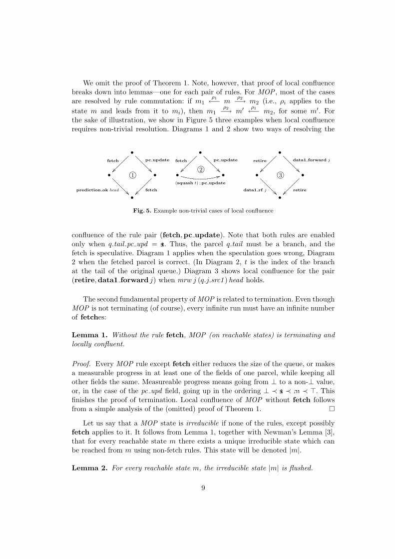
the sake of illustration, we show in Figure 5 three examples when local confluencerequires non-trivial resolution. Diagrams 1 and 2 show two ways of resolving the

•

fetch

ÄÄ~~~~~~~pc update

ÂÂ@@@@@@@

• '&%$Ã!"#1

prediction ok headÂÂ@@@@@@@ •

fetchÄÄ~~~~~~~

•

•

fetch

ÄÄ~~~~~~~pc update

ÂÂ@@@@@@@

•'&%$Ã!"#2

(squash t) ; pc update

44 •

•

retire

ÄÄ~~~~~~~data1 forward j

ÂÂ@@@@@@@

• '&%$Ã!"#3

data1 rf jÂÂ@@@@@@@ •

retireÄÄ~~~~~~~

•

Fig. 5. Example non-trivial cases of local confluence

confluence of the rule pair (fetch,pc update). Note that both rules are enabledonly when q.tail .pc upd = . Thus, the parcel q.tail must be a branch, and thefetch is speculative. Diagram 1 applies when the speculation goes wrong, Diagram2 when the fetched parcel is correct. (In Diagram 2, t is the index of the branchat the tail of the original queue.) Diagram 3 shows local confluence for the pair(retire,data1 forward j) when mrw j (q.j.src1 ) head holds.

The second fundamental property of MOP is related to termination. Even thoughMOP is not terminating (of course), every infinite run must have an infinite numberof fetches:

Lemma 1. Without the rule fetch, MOP (on reachable states) is terminating andlocally confluent.

Proof. Every MOP rule except fetch either reduces the size of the queue, or makesa measurable progress in at least one of the fields of one parcel, while keeping allother fields the same. Measureable progress means going from ⊥ to a non-⊥ value,or, in the case of the pc upd field, going up in the ordering ⊥ ≺ ≺ ≺ >. Thisfinishes the proof of termination. Local confluence of MOP without fetch followsfrom a simple analysis of the (omitted) proof of Theorem 1. ¤

Let us say that a MOP state is irreducible if none of the rules, except possiblyfetch applies to it. It follows from Lemma 1, together with Newman’s Lemma [3],that for every reachable state m there exists a unique irreducible state which canbe reached from m using non-fetch rules. This state will be denoted |m|.

Lemma 2. For every reachable state m, the irreducible state |m| is flushed.

9

Proof. Suppose the queue of |m| is not empty and let p be its head parcel. Weneed to consider separately the cases defined by the instruction class of p. All casesbeing similar, we will give a proof only for one: when p is a conditional branch. Sincedecode does not apply to it, pmust be fully decoded. Since data1 rf does not applyto p, we must have p.data 6= ⊥ (other conditions in the guard of data1 rf are true).Now, since branch taken and branch target do not apply, we can conclude thatp.res 6= ⊥ and p.tkn 6= ⊥. This, together with the fact that next pc branch doesnot apply, implies p.next pc 6= ⊥. Now, if p.pc upd = >, then retire would apply.Thus, we must have p.pc upd 6= >. Since pc update does not apply, the queuemust have length at least 2. If p.pc upd = , then either squash or prediction ok

would apply to the parcel p. Thus, p.pc upd is equal to ⊥ or , and this contradictsthe (easily checked) invariant saying that a parcel with p.pc upd equal to ⊥ or

must be at the tail of the queue. ¤

Define α(m) to be the ISA component of the flushed state |m|. Recall now thefunction γ defined at the beginning of this section. The functions γ and α map ISAstates to MOP states and the other way around. Clearly, α(γ(s)) = s.

The function α is analogous to the pipeline flushing functions of Burch-Dill [5].Indeed, we can prove that MOP satisfies the fundamental Burch-Dill correctnessproperty with respect to this flushing function.

Theorem 2. Suppose a MOP transition leads from m to m′, and m is reachable.Then α(m′) = isa step (α(m)) or α(m′) = α(m).

Proof. We can assume the transition m −→ m′ is a fetch; otherwise, we clearlyhave |m| = |m′|, and so α(m) = α(m′). The proof is by induction on the minimumlength k of a chain of (non-fetch) transitions from m to |m|. If k = 0, then m isflushed, so m = γ(s) for some ISA state s. By the discussion at the beginning ofSection 3, the fetch transition m −→ m′ is the first in a sequence that, without usingany further fetches, leads from γ(s) to γ(s′), where s′ = isa step s. It follows that|m′| = |γ(s′)|, so α(m′) = α(γ(s′)) = s′, as required.

mρ

//

fetch

²²

m1 // • . . . • // |m|

m′

σ

>>||||||||

mρ

//

fetch

²²

m1

fetch

²²

// • . . . • // |m|

m′σ // m′1

Fig. 6. Two cases for the inductive step in the proof of Theorem 2

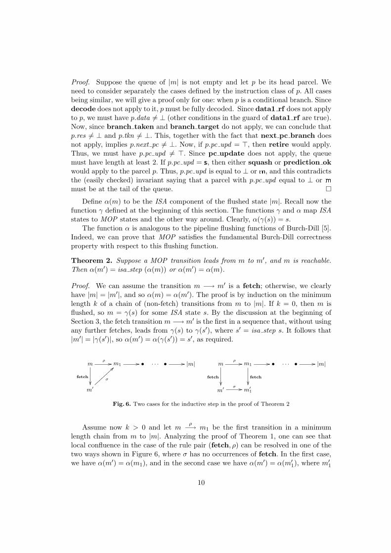
Assume now k > 0 and let mρ−→ m1 be the first transition in a minimum

length chain from m to |m|. Analyzing the proof of Theorem 1, one can see thatlocal confluence in the case of the rule pair (fetch, ρ) can be resolved in one of thetwo ways shown in Figure 6, where σ has no occurrences of fetch. In the first case,we have α(m′) = α(m1), and in the second case we have α(m′) = α(m′1), where m′1

10

is as in Figure 6. In the first case, we have α(m′) = α(m1) = α(m). In the secondcase, the proof follows from α(m) = α(m1), α(m′) = α(m′1), and the inductionhypothesis: α(m′1) = α(m1) or α(m′1) = isa step(α(m′1)). ¤

4 Simulating Microarchitectures in MOP

Suppose MA is a microarchitecture purportedly implementing the ISA. We will saythat a state-to-state map β from MA to MOP is a MOP-simulation if for every MAtransition s −→MA s′, the state β(s′) is reachable in MOP from β(s). Existence of aMOP -simulation proves (the safety part of) the correctness of MA. Indeed, for everyexecution sequence s1 −→MA s2 −→MA . . . , we have β(s1) −→+

MOPβ(s2) −→+

MOP

. . ., and then by Theorem 2, α(β(s1)) −→∗ISA

α(β(s2)) −→∗ISA

. . ., demonstratingthe crucial simulation relation between MA and ISA.

For a given MA, the MOP -simulation function β should be easy to guess. Thedifficult part is to verify that it satisfies the required property: the existence ofa chain of MOP transitions β(s) −→+

MOPβ(s′) for each transition s −→MA s′.

Somewhat simplistically, this verification task can be partitioned as follows.Suppose MA’s state variables are v1, . . . , vn. (Among them are the ISA state

variables, of course.) The MA transition function

s = 〈v1, . . . , vn〉 7−→ s′ = 〈v′1, . . . , v′n〉

is given by n functions next v i such that v′i = next v i 〈v1, . . . , vn〉. The n-step se-quence s = s0 Ã s1 Ã . . . Ã sn−1 Ã sn = s′ where si = 〈v′1, . . . , v

′i, vi+1, . . . , vn〉

conveniently serializes the parallel computation that MA does when it makes atransition from s to s′. These n steps are not MA transitions themselves since theintermediate si need not be legitimate MA states at all. However, it is reasonable toexpect that the progress described by this sequence is reflected in MOP by actualtransitions:

β(s) = m0 −→∗MOP m1 −→

∗MOP . . . −→∗MOP mn = β(s′). (1)

Defining the intermediate MOP states mi will usually be straightforward. Oncethey have been identified, the task of proving that β(s′) is reachable from β(s) isbroken down into n tasks of proving that mi+1 is reachable from mi. Effectively,the correctness of the MA next-state function is reduced to proving a correctnessproperty for each state component update function next v i.

5 Mechanization

Our method is intended to be used with a combination of interactive (or manual)and automated theorem proving. The correctness of the MOP system (Theorem 2)rests largely on its local confluence (Theorem 1), which is naturally and easily splitinto a large number of cases that can be individually verified by an automated SMT

11

solver. The solver needs decision procedures for uninterpreted functions, a fragmentof arithmetic, and common datatypes auch as arrays, records and enumeration types.Once the MA-simulation function β of Section 4 has been defined and the intermedi-ate MOP states mi in the chain (1) identified, it should also be possible to generatethe proof of reachability of mi+1 from mi with the aid of the same solver.

We have used manual proof decomposition and CVC Lite to implement theproof procedure just described. Our models for ISA, MOP , and MA are all writtenin the reflective general-purpose functional language reFLect [7]. In this convenientframework we can execute specifications and—through a HOL-like theorem proveron top of reFLect or an integrated CVC Lite—formally reason about them at thesame time. Local confluence of MOP is (to some extent automatically) reduced toabout 400 goals, which are individually proved with CVC Lite. For MA we used thetextbook DLX model [9] and proved it is simulated in MOP by constructing thechains (1) and verifying them with CVC Lite. This proof is sketched in some detailin the Appendix.

Mechanization of our method is still in progress. Clean and efficient use of SMTsolvers to prove properties of executable high-level models written in another lan-guage comes with challenges, some of which were discussed in [8]. For us, particularlyexigent is the demand for heuristics for deciding when to expand occurrences of func-tion symbols in goals passed to the SMT solver with the functions’ definitions, andwhen to treat them as uninterpreted.

6 Related Work

The idea of flushing a pipeline automatically was introduced in a seminal paper byBurch and Dill [5]. In the original approach, all in-flight instructions in the imple-mentation state are flushed out of the pipeline by inserting bubbles—NOPs that donot affect the program counter. Pipelines that use a combination of super-scalar exe-cution, out-of-order execution, variable-latency execution units, etc. are too complexto flush directly. In response, researchers have invented a variety of ways, many basedon flushing, to relate the implementation pipeline to the specification. We cover hereonly those approaches that are most closely related. The interested reader is referedto [1] for a relatively complete survey of pipeline verification approaches.

Damm and Pnueli [6] use a non-deterministic specification that generates allprogram traces that satisfy data dependencies. They use an intermediate abstractionwith auxiliary variables to relate the specification and an implementation with out-of-order retirement based on Tomasulo’s algorithm. In each step of the specificationmodel, an entire instruction is executed atomically and its result written back. Inthe MOP approach, the execution of each instruction is broken into a sequence ofmini-steps in order to relate to a pipelined implementation.

Skakkebæk et al. [16, 11] introduce incremental flushing and use a non-determini-stic intermediate model to prove correctness of a simple out-of-order core with in-order retirement. Like us, they rely on arguments about re-ordering transactions.

12

While incremental flushing must deal with transactions as they are defined for thepipeline, we decompose pipeline transactions into much simpler “atomic” transac-tions. This facilitates a more general abstraction and should require significantlyless manual proof effort than the incremental flushing approach.

Sawada and Hunt [14] use an intermediate model with an unbounded history ta-ble called a micro-architectural execution trace table. It contains instruction-specificinformation similar to that found in the MOP queue. Arons [2] follows a similarpath, augmenting an implementation model with history variables that record thepredicted results of instruction execution. In these approaches, auxiliary state is—like the MOP queue—employed to derive and prove invariants about the implemen-tation’s relation to the specification. While their auxiliary state is derived directlyfrom the MA, MOP is largely independent of MA and has fine-grained transitions.

Arvind and Shen [15] use term rewriting to model an out-of-order processor andits specification. Similar to our approach, multiple rewrite rules may be requiredto complete an implementation step. As in the current approach, branch predictionis modeled by non-determinism. In contrast with the current approach, a singleprocessor implementation is related directly to its in-order specification.

Hosabettu et al. [10] devised a method to decompose the Burch-Dill correctnessstatement into lemmas, one per pipeline stage. This inspired the decomposition wedescribe in Section 4.

Lahiri and Bryant [12], and Manolios and Srinivasan [13] verified complex mi-croprocessor models using the SMT solver UCLID. Some consistency invariants in[12] occur naturally in our confluence proofs as well, but the overall approach isnot closely related. The WEB-refinement method used in [13] produces proofs ofstrong correspondence between ISA and MA (stuttering bisimulation) that impliesliveness. We have proved that MOP with a bounded queue and ISA are stutteringequivalent, also establishing liveness. The proof is contained in the Appendix.

7 Conclusion

We have presented a new approach for verifying a pipelined system P against itsspecification S by using an intermediate “pipeline mother” systemM that explicatesatomic computations occurring in steps of S. For definiteness, we assumed that P isa microprocessor model and S is its ISA, but the method can potentially be appliedto verify pipelined hardware components in general, or in protocol verification. Thiscan all be seen as a refinement of the classical Burch-Dill method, but with thedifficult flushing-based simulation pushed to theM vs. S level, where it amounts toproving local confluence of M—a conjunction of easily-stated properties of limitedsize, readily verifiable by SMT solvers.

As an example, we specified a concrete intermediate model MOP for a simpleload-store architecture and proved its correctness. We also verified the textbookmachine DLX against it. However, our MOP contains more than is needed forverifying DLX : it is designed for simulation of microprocessor models with complex

13

out-of-order execution that cannot be handled by currently available methods. Thiswill be addressed in future work. Also left for future work are improvements toour methodology (manual decomposition of verification goals into subgoals whichwe prove with CVC Lite [4]) and performance comparison with other publishedmethods.

Acknowledgment. We thank Jesse Bingham for his comments.

References

1. M. D. Aagaard, B. Cook, N. A. Day, and R. B. Jones. A framework for superscalar micropro-cessor correctness statements. Software Tools for Technology Transfer, 4(3):298–312, 2003.

2. T. Arons. Verification of an advanced MIPS-type out-of-order execution algorithm. In Com-puter Aided Verification (CAV’04), volume 3114 of LNCS, pages 414–426, 2004.

3. F. Baader and T. Nipkow. Term Rewriting and All That. Cambridge University Press, 1998.4. C. Barrett and S. Berezin. CVC Lite: A new implementation of the cooperating validity checker.

In R. Alur and D. A. Peled, editors, Computer Aided Verification (CAV’04), volume 3114 ofLNCS, pages 515–518, 2004.

5. J. Burch and D. Dill. Automatic verification of pipelined microprocessor control. In D. L. Dill,editor, Computer Aided Verification (CAV’94), volume 818 of LNCS, pages 68–80, 1994.

6. W. Damm and A. Pnueli. Verifying out-of-order executions. In H. F. Li and D. K. Probst,editors, Correct Hardware Design and Verification Methods (CHARME’97), pages 23–47. Chap-man and Hall, 1997.

7. J. Grundy, T. Melham, and J. O’Leary. A reflective functional language for hardware designand theorem proving. J. Functional Programming, 16(2):157–196, 2006.

8. J. Grundy, T. F. Melham, S. Krstic, and S. McLaughlin. Tool building requirements for anAPI to first-order solvers. Electr. Notes Theor. Comput. Sci., 144(2):15–26, 2006.

9. J. Hennessy and D. Patterson. Computer Architecture: A Quantitative Approach. MorganKaufmann, 1995.

10. R. Hosabettu, G. Gopalakrishnan, and M. Srivas. Verifying advanced microarchitectures thatsupport speculation and exceptions. In E. A. Emerson and A. P. Sistla, editors, ComputerAided Verification (CAV’00), volume 1855 of LNCS, pages 521–537, 2000.

11. R. B. Jones. Symbolic Simulation Methods for Industrial Formal Verification. Kluwer, 2002.12. S. K. Lahiri and R. E. Bryant. Deductive verification of advanced out-of-order microprocessors.

In W. A. Hunt Jr. and F. Somenzi, editors, Computer Aided Verification (CAV’03), volume2725 of LNCS, pages 341–354, 2003.

13. P. Manolios and S. K. Srinivasan. A complete compositional reasoning framework for the effi-cient verification of pipelined machines. In IEEE/ACM International conference on Computer-aided design (ICCAD’05), pages 863–870. IEEE Computer Society, 2005.

14. J. Sawada and W. Hunt. Processor verification with precise exceptions and speculative exe-cution. In Alan J. Hu and Moshe Y. Vardi, editors, Computer Aided Verification (CAV’98),volume 1427 of LNCS, pages 135–146, 1998.

15. X. Shen and Arvind. Design and verification of speculative processors. In Workshop on FormalTechniques for Hardware, Maarstrand, Sweden, June 1998.

16. J. Skakkebæk, R. Jones, and D. Dill. Formal verification of out-of-order execution using in-cremental flushing. In Alan J. Hu and Moshe Y. Vardi, editors, Computer Aided Verification(CAV’98), volume 1427 of LNCS, pages 98–109, 1998.

14

Applications of hierarchical reasoning in

the verification of complex systems

Swen Jacobs and Viorica Sofronie-Stokkermans

Max-Planck-Institut fur Informatik, Stuhlsatzenhausweg 85, Saarbrucken, Germany

e-mail: sjacobs, sofronie@mpi-sb.mpg.de

Abstract

In this paper we show how hierarchical reasoning can be used toverify properties of complex systems. Chains of local theory extensionsare used to model a case study taken from the European Train ControlSystem (ETCS) standard, but considerably simplified. We show howtesting invariants and bounded model checking can automatically bereduced to checking satisfiability of ground formulae over a base theory.

1 Introduction

Many problems in computer science can be reduced to proving satisfiabilityof conjunctions of (ground) literals modulo a background theory. This theorycan be a standard theory, the extension of a base theory with additionalfunctions (free or subject to additional conditions), or a combination oftheories. In [8] we showed that for special types of theory extensions, whichwe called local, hierarchic reasoning in which a theorem prover for the basetheory is used as a “black box” is possible. Many theories important forcomputer science are local extensions of a base theory. Several examples(including theories of data structures, e.g. theories of lists (or arrays cf. [3]);but also theories of monotone functions or of functions satisfying semi-Galoisconditions) are given in [8] and [9]. Here we present additional examples oflocal theory extensions occurring in the verification of complex systems.

In this paper we address a case study taken from the specification ofthe European Train Control System (ETCS) standard [2], but considerablysimplified, namely an example of a communication device responsible fora given segment of the rail track, where trains may enter and leave. Wesuppose that, at fixed moments in time, all knowledge about the currentpositions of the trains is available to a controller which accordingly imposesconstraints on the speed of some trains, or allows them to move freely withinthe allowed speed range on the track. Related problems were tackled beforewith methods from verification [2].

The approach we use in this paper is different from previously usedmethods. We use sorted arrays (or monotonely decreasing functions) forstoring the train positions. The use of abstract data structures allows us to

15

pass in an elegant way from verification of several finite instances of problems(modeled by finite-state systems) to general verification results, in which setsof states are represented using formulae in first-order logic, by keeping thenumber of trains as a parameter. We show that for invariant or boundedmodel checking the specific properties of “position updates” can be expressedin a natural way by using chains of local theory extensions. Therefore we canuse results in hierarchic theorem proving both for invariant and for boundedmodel checking1. By using locality of theory extensions we also obtainedformal arguments on possibilities of systematic “slicing” (for bounded modelchecking): we show that for proving (disproving) the violation of the safetycondition we only need to consider those trains which are in a ’neighborhood’of the trains which violate the safety condition2.

Structure of the paper. Section 2 contains the main theoretical results neededin the paper. In Section 3 we describe the case study we consider. In Sec-tion 4 we present a method for invariant and bounded model checking basedon hierarchical reasoning. Section 5 contains conclusions and perspectives.

2 Preliminaries

Theories and models. Theories can be regarded as sets of formulae oras sets of models. Let T be a theory in a (many-sorted) signature Π =(S,Σ,Pred), where S is a set of sorts, Σ is a set of function symbols andPred a set of predicate symbols (with given arities). A Π-structure is a tuple

M = (Mss∈S , fMf∈Σ, PMP∈Pred),

where for every s ∈ S, Ms is a non-empty set, for all f ∈ Σ with aritya(f)=s1. . .sn → s, fM :

∏ni=1

Msi→Ms and for all P ∈ Pred with aritya(P ) = s1. . .sn, PM ⊆Ms1× . . .×Msn . We consider formulae over variablesin a (many-sorted) family X = Xs | s ∈ S, where for every s ∈ S, Xs is aset of variables of sort s. A model of T is a Π-structure satisfying all formulaeof T . In this paper, whenever we speak about a theory T we implicitly referto the set Mod(T ) of all models of T , if not otherwise specified.

Partial structures. Let T0 be a theory with signature Π0 = (S0,Σ0,Pred).We consider extensions T1 of T0 with signature Π = (S,Σ,Pred), whereS = S0 ∪ S1,Σ = Σ0 ∪ Σ1 (i.e. the signature is extended by new sortsand function symbols) and T1 is obtained from T0 by adding a set K of(universally quantified) clauses. Thus, Mod(T1) consists of all Π-structureswhich are models of K and whose reduct to Π0 is a model of T0.

A partial Π-structure is a structureM = (Mss∈S , fMf∈Σ, PMP∈Pred),where for every s ∈ S, Ms is a non-empty set and for every f ∈ Σ with arity

1Here we only focus on one example. However, we also used this technique for othercase studies (among which one is mentioned – in a slightly different context – in [9]).

2In fact, it turns out that slicing (locality) results with a similar flavor presented byNecula and McPeak in [6] have a similar theoretical justification.

16

s1 . . . sn → s, fM is a partial function from Ms1 × · · · ×Msn to Ms. Thenotion of evaluating a term t with variables X = Xs | s ∈ S w.r.t. anassignment βs:Xs →Ms | s ∈ S for its variables in a partial structure Mis the same as for total many-sorted algebras, except that this evaluationis undefined if t = f(t1, . . . , tn) with a(f) = (s1 . . . sn → s), and at leastone of βsi(ti) is undefined, or else (βs1(t1), . . . , βsn(tn)) is not in the domainof fM. In what follows we will denote a many-sorted variable assignmentβs:Xs → Ms | s ∈ S as β : X →M. Let M be a partial Π-structure, Ca clause and β : X →M. We say that (M, β) |=w C iff either (i) for someterm t in C, β(t) is undefined, or else (ii) β(t) is defined for all terms t of C,and there exists a literal L in C s.t. β(L) is true in M. M weakly satisfiesC (notation: M |=w C) if (M, β) |=w C for all assignments β. M weaklysatisfies (is a weak partial model of) a set of clauses K (notation: M |=w K,M is a w.p.model of K) if M |=w C for all C ∈ K.

Local theory extensions. Let K be a set of (universally quantified) clausesin the signature Π = (S,Σ,Pred), where S = S0 ∪ S1 and Σ = Σ0 ∪ Σ1. Inwhat follows, when referring to sets G of ground clauses we assume they arein the signature Πc = (S,Σ ∪ Σc,Pred) where Σc is a set of new constants.An extension T0 ⊆ T0 ∪ K is local if satisfiability of a set G of clauses withrespect to T0∪K, only depends on T0 and those instances K[G] of K in whichthe terms starting with extension functions are in the set st(K, G) of groundterms which already occur in G or K. Formally,

K[G] = Cσ |C ∈ K, for each subterm f(t) of C, with f ∈ Σ1,

f(t)σ ∈ st(K, G), and for each variable x which does notoccur below a function symbol in Σ1, σ(x) = x,

and T0 ⊆ T1=T0 ∪ K is a local extension if it satisfies condition (Loc):

(Loc) For every set G of ground clauses G |=T1⊥ iff there is no partialΠc-structure P such that P|Π0

is a total model of T0, all terms

in st(K, G) are defined in P , and P weakly satisfies K[G] ∧G.

In [8, 9] we gave several examples of local theory extensions: e.g. any ex-tension of a theory with free function symbols; extensions with selectorfunctions for a constructor which is injective in the base theory; extensionsof several partially ordered theories with monotone functions. In Section 4.2we give additional examples which have particular relevance in verification.

Hierarchic reasoning in local theory extensions. Let T0 ⊆ T1=T0 ∪Kbe a local theory extension. To check the satisfiability of a set G of groundclauses w.r.t. T1 we can proceed as follows (for details cf. [8]):

Step 1: Use locality. By the locality condition, G is unsatisfiable w.r.t. T1 iffK[G] ∧G has no weak partial model in which all the subterms of K[G] ∧Gare defined, and whose restriction to Π0 is a total model of T0.

17

Step 2: Flattening and purification. We purify and flatten K[G] ∧ G byintroducing new constants for the arguments of the extension functions aswell as for the (sub)terms t = f(g1, . . . , gn) starting with extension functionsf ∈ Σ1, together with new corresponding definitions ct ≈ t. The set ofclauses thus obtained has the form K0 ∧G0 ∧D, where D is a set of groundunit clauses of the form f(c1, . . . , cn) ≈ c, where f ∈ Σ1 and c1, . . . , cn, c areconstants, and K0, G0 are clause sets without function symbols in Σ1.

Step 3: Reduction to testing satisfiability in T0. We reduce the problem totesting satisfiability in T0 by replacing D with the following set of clauses:

N0 =∧

n∧

i=1

ci≈di→c≈d | f(c1, . . . , cn) = c, f(d1, . . . , dn) = d ∈ D.

Theorem 1 ([8]) With the notations above, the following are equivalent:

(1) T0 ∧ K ∧G has a model.

(2) T0∧K[G]∧G has a w.p.model (where all terms in st(K,G) are defined).

(3) T0∧K0∧G0∧D has a w.p.model (with all terms in st(K,G) defined).

(4) T0∧K0∧G0∧N0 has a (total) Σ0-model.

3 The RBC Case Study

The case study we discuss here is taken from the specification of the Eu-ropean Train Control System (ETCS) standard: we consider a radio blockcenter (RBC), which communicates with all trains on a given track segment.Trains may enter and leave the area, given that a certain maximum numberof trains on the track is not exceeded. Every train reports its position tothe RBC in given time intervals and the RBC communicates to every trainhow far it can safely move, based on the position of the preceding train. Itis then the responsibility of the trains to adjust their speed between givenminimum and maximum speeds.

For a first try at verifying properties of this system, we have considerablysimplified it: we abstract from the communication issues in that we alwaysevaluate the system after a certain time ∆t, and at these evaluation pointsthe positions of all trains are known. Depending on these positions, thepossible speed of every train until the next evaluation is decided: if thedistance to the preceding train is less than a certain limit lalarm, the trainmay only move with minimum speed min (otherwise with any speed betweenmin and the maximum speed max).

3.1 Formal Description of the System Model

We present two formal system models. In the first one we have a fixednumber of trains; in the second we allow for entering and leaving trains.

Model 1: Fixed Number of Trains. In this simpler model, any state ofthe system is characterized by the following functions and constants:

18

• ∆t > 0, the time between evaluations of the system.

• min and max, the minimum and maximum speed of trains. We assumethat 0 ≤ min ≤ max.

• lalarm, the distance between trains which is deemed secure.

• n, the number of trains.

• pos, a function which maps indices (between 0 and n−1) associated totrains on the track to the positions of those trains on the track. Herepos(i) denotes the current position of the train with index i.

We use a new function pos′ to model the evolution of the system: pos′(i)denotes the position of i at the next evaluation point (after ∆t time units).The way positions change (i.e. the relationship between pos and pos′) isdefined by the following set Kf = F1,F2,F3,F4 of axioms:

(F1) ∀i (i = 0 → pos(i) + ∆t∗min ≤R pos′(i) ≤R pos(i) + ∆t∗max)

(F2) ∀i (0 < i < n ∧ pos(i− 1) >R 0 ∧ pos(p(i))− pos(i) ≥R lalarm

→ pos(i) + ∆t ∗min ≤R pos′(i) ≤R pos(i) + ∆t∗max)

(F3) ∀i (0 < i < n ∧ pos(i− 1) >R 0 ∧ pos(p(i))− pos(i) <R lalarm

→ pos′(i) = pos(i) + ∆t∗min)

(F4) ∀i (0 < i < n ∧ pos(i− 1) ≤R 0 → pos′(i) = pos(i)),

Note that the train with number 0 is the train with the greatest position,i.e. we count trains from highest to lowest position.

Axiom F1 states that the first train may always move at any speedbetween min and max. F2 states that the other trains can do so if theirpredecessor has already started and the distance to it is larger than lalarm.If the predecessor of a train has started, but is less than lalarm away, thenthe train may only move at speed min (axiom F3). F4 requires that a trainmay not move at all if its predecessor has not started.

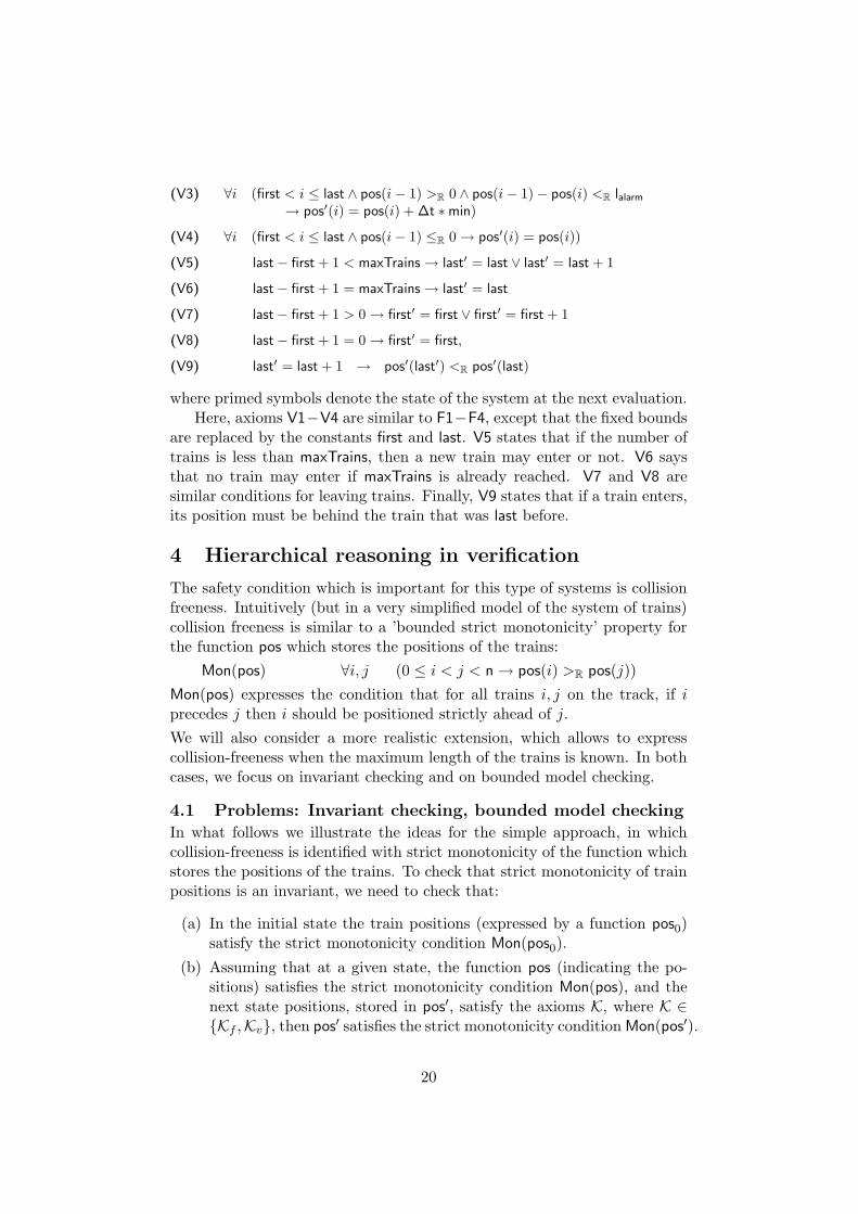
Model 2: Incoming and leaving trains. If we allow incoming andleaving trains, we additionally need a measure for the number of trains onthe track. This is given by additional constants first and last, which at anytime give the number of the first and last train on the track (again, the firsttrain is supposed to be the train with the highest position). Furthermore, themaximum number of trains that is allowed to be on the track simultaneouslyis given by a constant maxTrains. These three values replace the number oftrains n in the simpler model, the rest of it remains the same except that thefunction pos is now defined for values between first and last, where before itwas defined between 0 and n − 1. The behavior of this extended system isdescribed by the following set Kv consisting of axioms (V1)− (V9):

(V1) ∀i (i = first→ pos(i) + ∆t ∗min ≤R pos′(i) ≤R pos(i) + ∆t ∗max)

(V2) ∀i (first < i ≤ last ∧ pos(i− 1) >R 0 ∧ pos(i− 1)− pos(i) ≥R lalarm

→ pos(i) + ∆t ∗min ≤R pos′(i) ≤R pos(i) + ∆t ∗max)

19

(V3) ∀i (first < i ≤ last ∧ pos(i− 1) >R 0 ∧ pos(i− 1)− pos(i) <R lalarm

→ pos′(i) = pos(i) + ∆t ∗min)

(V4) ∀i (first < i ≤ last ∧ pos(i− 1) ≤R 0→ pos′(i) = pos(i))

(V5) last− first + 1 < maxTrains→ last′ = last ∨ last′ = last + 1

(V6) last− first + 1 = maxTrains→ last′ = last

(V7) last− first + 1 > 0→ first′ = first ∨ first′ = first + 1

(V8) last− first + 1 = 0→ first′ = first,

(V9) last′ = last + 1 → pos′(last′) <R pos′(last)

where primed symbols denote the state of the system at the next evaluation.Here, axioms V1−V4 are similar to F1−F4, except that the fixed bounds

are replaced by the constants first and last. V5 states that if the number oftrains is less than maxTrains, then a new train may enter or not. V6 saysthat no train may enter if maxTrains is already reached. V7 and V8 aresimilar conditions for leaving trains. Finally, V9 states that if a train enters,its position must be behind the train that was last before.

4 Hierarchical reasoning in verification

The safety condition which is important for this type of systems is collisionfreeness. Intuitively (but in a very simplified model of the system of trains)collision freeness is similar to a ’bounded strict monotonicity’ property forthe function pos which stores the positions of the trains:

Mon(pos) ∀i, j (0 ≤ i < j < n→ pos(i) >R pos(j))

Mon(pos) expresses the condition that for all trains i, j on the track, if iprecedes j then i should be positioned strictly ahead of j.

We will also consider a more realistic extension, which allows to expresscollision-freeness when the maximum length of the trains is known. In bothcases, we focus on invariant checking and on bounded model checking.

4.1 Problems: Invariant checking, bounded model checking

In what follows we illustrate the ideas for the simple approach, in whichcollision-freeness is identified with strict monotonicity of the function whichstores the positions of the trains. To check that strict monotonicity of trainpositions is an invariant, we need to check that:

(a) In the initial state the train positions (expressed by a function pos0)satisfy the strict monotonicity condition Mon(pos0).

(b) Assuming that at a given state, the function pos (indicating the po-sitions) satisfies the strict monotonicity condition Mon(pos), and thenext state positions, stored in pos′, satisfy the axioms K, where K ∈Kf ,Kv, then pos′ satisfies the strict monotonicity condition Mon(pos′).

20

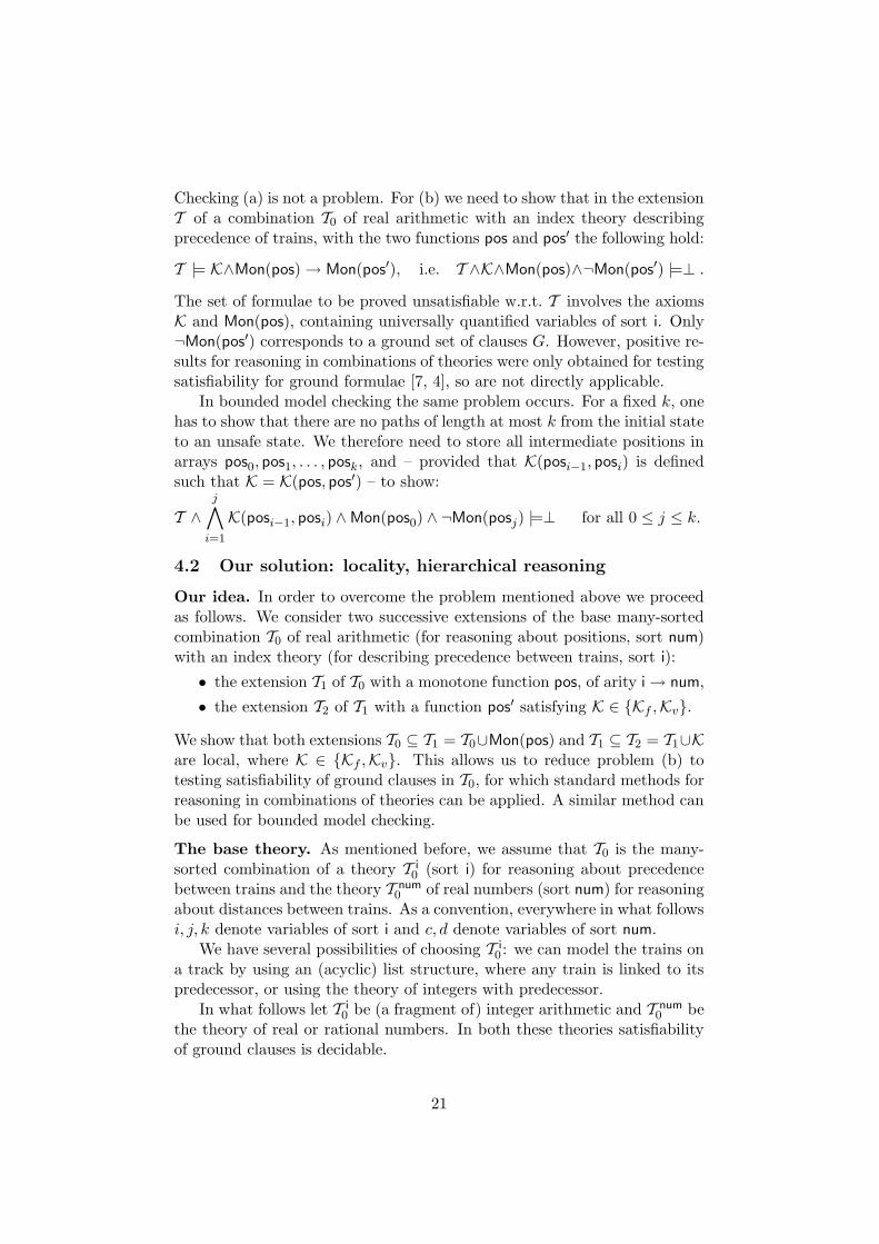
Checking (a) is not a problem. For (b) we need to show that in the extensionT of a combination T0 of real arithmetic with an index theory describingprecedence of trains, with the two functions pos and pos′ the following hold:

T |= K∧Mon(pos)→ Mon(pos′), i.e. T ∧K∧Mon(pos)∧¬Mon(pos′) |=⊥ .

The set of formulae to be proved unsatisfiable w.r.t. T involves the axiomsK and Mon(pos), containing universally quantified variables of sort i. Only¬Mon(pos′) corresponds to a ground set of clauses G. However, positive re-sults for reasoning in combinations of theories were only obtained for testingsatisfiability for ground formulae [7, 4], so are not directly applicable.

In bounded model checking the same problem occurs. For a fixed k, onehas to show that there are no paths of length at most k from the initial stateto an unsafe state. We therefore need to store all intermediate positions inarrays pos0, pos1, . . . , posk, and – provided that K(posi−1, posi) is definedsuch that K = K(pos, pos′) – to show:

T ∧

j∧

i=1

K(posi−1, posi) ∧Mon(pos0) ∧ ¬Mon(posj) |=⊥ for all 0 ≤ j ≤ k.

4.2 Our solution: locality, hierarchical reasoning

Our idea. In order to overcome the problem mentioned above we proceedas follows. We consider two successive extensions of the base many-sortedcombination T0 of real arithmetic (for reasoning about positions, sort num)with an index theory (for describing precedence between trains, sort i):

• the extension T1 of T0 with a monotone function pos, of arity i→ num,

• the extension T2 of T1 with a function pos′ satisfying K ∈ Kf ,Kv.

We show that both extensions T0 ⊆ T1 = T0∪Mon(pos) and T1 ⊆ T2 = T1∪Kare local, where K ∈ Kf ,Kv. This allows us to reduce problem (b) totesting satisfiability of ground clauses in T0, for which standard methods forreasoning in combinations of theories can be applied. A similar method canbe used for bounded model checking.

The base theory. As mentioned before, we assume that T0 is the many-sorted combination of a theory T i

0(sort i) for reasoning about precedence

between trains and the theory T num0

of real numbers (sort num) for reasoningabout distances between trains. As a convention, everywhere in what followsi, j, k denote variables of sort i and c, d denote variables of sort num.

We have several possibilities of choosing T i0: we can model the trains on

a track by using an (acyclic) list structure, where any train is linked to itspredecessor, or using the theory of integers with predecessor.

In what follows let T i0

be (a fragment of) integer arithmetic and T num0

bethe theory of real or rational numbers. In both these theories satisfiabilityof ground clauses is decidable.

21

Collision freeness as monotonicity. Let T0 be the (disjoint, many-sorted) combination of T i

0and T num

0. Then classical methods on combina-

tions of decision procedures for (disjoint, many-sorted) theories can be usedto give a decision procedure for satisfiability of ground clauses w.r.t. T0. LetT1 be obtained by extending T0 with a function pos of arity i→ num mappingtrain indices to the real numbers, which satisfies condition Mon(pos):

Mon(pos) ∀i, j (first ≤ i < j ≤ last→ pos(i) >R pos(j)),

where i and j are indices, < is the ordering on indices and >R is the usualordering on the real numbers. (For the case of a fixed number of trains, wecan assume that first = 0 and last = n− 1.)

A more precise axiomatization of collision-freeness. The monotonic-ity axiom above is, in fact, an oversimplification. A more precise model, inwhich the length of trains is considered can be obtained by replacing themonotonicity axiom for pos with the following axiom:

∀i, j, k (first ≤ j ≤ i ≤ last∧ i− j = k → pos(j)−pos(i) ≥ k ∗LengthTrain),

where LengthTrain is the standard (resp. maximal) length of a train.As base theory we consider the combination T ′

0of the theory of inte-

gers and reals with a multiplication operation ∗ of arity i × num → num(multiplication of k with the constant LengthTrain in the formula above)3.

Let T ′1

be the theory obtained by extending the combination T ′0

of thetheory of integers and reals with a function pos satisfying the axiom above.

Theorem 2 The following extensions are local theory extensions:

(1) The theory extension T0 ⊆ T1.

(2) The theory extension T ′0⊆ T ′

1.

Proof : We prove that every model of T1 in which the function pos is partiallydefined can be extended to a model in which pos is totally defined. Localitythen follows by results in [8]. To define pos at positions where it is undefinedwe use the density of real numbers and the discreteness of the index theory(between two integers there are only finitely many integers). 2

We now extend the resulting theory T1 again in two different ways, withthe axiom sets for one of the two system models, respectively. A similarconstruction can be done starting from the theory T ′

1.

Theorem 3 The following extensions are local theory extensions:

(1) The extension T1 ⊆ T1 ∪ Kf(2) The extension T1 ⊆ T1 ∪ Kv.

3In the light of locality properties of such extensions (cf. Theorem 2), k will always beinstantiated by values in a finite set of concrete integere, all within a given, concrete range;thus the introduction of this many-sorted multiplication does not affect decidability.

22

Proof : (1) Clauses in Kf are flat and linear w.r.t. pos′, so we again prove lo-cality of the extension by showing that weak partial models can be extendedto total ones. The proof proceeds by a case distinction. We use the fact thatthe left-hand sides of the implications in Kf are mutually exclusive. (2) isproved similarly. 2

Let K ∈ Kv,Kf. By the locality of T1 ⊆ T2 = T1 ∪ K and by Theorem 1,the following are equivalent:

(1) T0 ∧Mon(pos) ∧ K ∧ ¬Mon(pos′) |=⊥,

(2) T0 ∧Mon(pos) ∧ K[G] ∧G |=w⊥, where G = ¬Mon(pos′),

(3) T0 ∧Mon(pos) ∧ K0 ∧G0 ∧N0(pos′) |=⊥,

where K[G] consists of all instances of the rules in K in which the terms start-ing with the function symbols pos′ are ground subterms already occurringin G or K, K0 ∧G0 is obtained from K[G]∧G by introducing new constantsfor the arguments of the extension functions as well as for the (sub)termst = f(g1, . . . , gn) starting with extension functions f ∈ Σ1, and N0(pos′) isthe set of instances of the congruence axioms for pos′ which correspond tothe definitions for these newly introduced constants.

It is easy to see that, due to the special form of the rules in K (all freevariables in any clause occur as arguments of pos′ both in Kf and in Kv),K[G] (hence also K0) is a set of ground clauses. By the locality of T0 ⊆ T1 =T0 ∪Mon(pos), the following are equivalent:

(1) T0 ∧Mon(pos) ∧ K0 ∧G0 ∧N0(pos′) |=⊥,

(2) T0 ∧Mon(pos)[G′] ∧G′ |=w⊥, where G′ = K0 ∧G0 ∧N0(pos′),

(3) T0 ∧Mon(pos)0 ∧G′0∧N0(pos) |=⊥,

where Mon(pos)[G′] consists of all instances of the rules in Mon(pos) inwhich the terms starting with the function symbol pos are ground subtermsalready occurring inG′, Mon(pos)0∧G

′0

is obtained from Mon(pos)[G′]∧G′ bypurification and flattening, and N0(pos) corresponds to the set of instancesof congruence axioms for pos which need to be taken into account.

This allows us to use hierarchical reasoning on properties of the system, i.e.to reduce the verification of system properties to deciding satisfiability ofconstraints in T0. An advantage is that, after the reduction of the problem toa satisfiability problem in the base theory, one can automatically determinewhich constraints on the parameters (e.g. ∆t,min,max, ...) guarantee truthof the invariant. This can be achieved, e.g. using quantifier elimination. Themethod is illustrated in Section 4.3; more details can be found in [5].

Similar results can be established for bounded model checking. In this casethe arguments are similar, but one needs to consider chains of extensionsof length 1, 2, 3, . . . , k for a bounded k, corresponding to the paths from

23

the initial state to be analyzed. An interesting side-effect of our approach(restricting to instances which are similar to the goal) is that it provides apossibility of systematic “slicing”: for proving (disproving) the violation ofthe safety condition we only need to consider those trains which are in a’neighborhood’ of the trains which violate the safety condition.

4.3 Illustration

In this section we indicate how to apply hierarchical reasoning on the casestudy given in Section 3, Model 1. We follow the steps given at the end ofSection 2 and show how the sets of formulas are obtained that can finallybe handed to a prover of the base theory T0.

To check whether T1 ∪ Kf |= ColFree(pos′), where

ColFree(pos′) ∀i (0 ≤ i < n− 1 → pos′(i) >R pos′(i+ 1)),

we check whether T1 ∪ Kf ∪ G |= ⊥, where G = 0 ≤ k < n − 1, k′ =k + 1, pos′(k) ≤R pos′(k′) is the (skolemized) negation of ColFree(pos′),flattened by introducing a new constant k′. This problem is reduced to asatisfiability problem over T1 as follows:

Step 1: Use locality. We construct the set Kf [G]: There are no groundsubterms with pos′ at the root in Kf , and only two ground terms with pos′

in G, pos′(k) and pos′(k′). This means that Kf [G] consists of two instancesof Kf : one with i instantiated to k, the other instantiated to k′. E.g., thetwo instances of F2 are:

(F2[G]) (0 < k < n ∧ pos(k − 1) >R 0 ∧ pos(k − 1)− pos(k) ≥R lalarm

→ pos(k) + ∆t ∗min ≤R pos′(k) ≤R pos(k) + ∆t∗max)(0 < k′ < n ∧ pos(k′ − 1) >R 0 ∧ pos(k′ − 1)− pos(k′) ≥R lalarm

→ pos(k′) + ∆t ∗min ≤R pos′(k′) ≤R pos(k′) + ∆t∗max)

The construction of (F1[G]), (F3[G]) and (F4[G]) is similar. In addition, wespecify the known relationships between the constants of the system:(Dom) ∆t > 0 ∧ 0 ≤ min ∧ min ≤ max

Step 2: Flattening and purification. Kf [G] ∧ G is already flat w.r.t.pos′. We replace all ground terms with pos′ at the root with new constants:we replace pos′(k) by c1 and pos′(k′) by c2. We obtain a set of definitionsD = pos′(k) = c1, pos′(k′) = c2 and a set Kf0

of clauses which do notcontain occurrences of pos′, consisting of (Dom) together with:

(G0) 0 ≤ k < n− 1 ∧ k′ = k + 1 ∧ c1 ≤R c2

(F20) (0 < k < n ∧ pos(k − 1) >R 0 ∧ pos(k − 1)− pos(k) ≥R lalarm

→ pos(k) + ∆t ∗min ≤R c1 ≤R pos(k) + ∆t∗max)

(0 < k′ < n ∧ pos(k′ − 1) >R 0 ∧ pos(k′ − 1)− pos(k′) ≥R lalarm

→ pos(k′) + ∆t ∗min ≤R c2 ≤R pos(k′) + ∆t∗max)

The construction can be continued similarly for F1, F3 and F4.

24

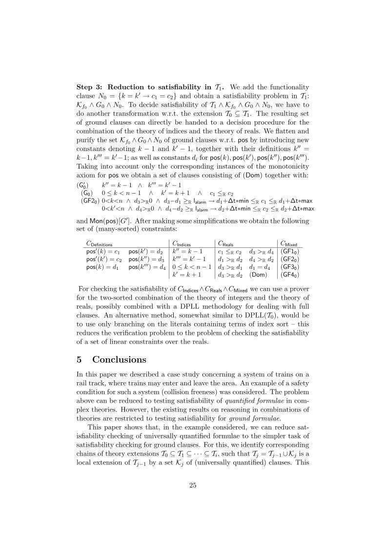
Step 3: Reduction to satisfiability in T1. We add the functionalityclause N0 = k = k′ → c1 = c2 and obtain a satisfiability problem in T1:Kf0∧ G0 ∧ N0. To decide satisfiability of T1 ∧ Kf0

∧ G0 ∧ N0, we have todo another transformation w.r.t. the extension T0 ⊆ T1. The resulting setof ground clauses can directly be handed to a decision procedure for thecombination of the theory of indices and the theory of reals. We flatten andpurify the set Kf0

∧G0∧N0 of ground clauses w.r.t. pos by introducing newconstants denoting k − 1 and k′ − 1, together with their definitions k′′ =k−1, k′′′ = k′−1; as well as constants di for pos(k), pos(k′), pos(k′′), pos(k′′′).Taking into account only the corresponding instances of the monotonicityaxiom for pos we obtain a set of clauses consisting of (Dom) together with:

(G′0) k′′ = k − 1 ∧ k′′′ = k′ − 1

(G0) 0 ≤ k < n− 1 ∧ k′ = k + 1 ∧ c1 ≤R c2(GF20) 0<k<n ∧ d3>R0 ∧ d3−d1 ≥R lalarm → d1+∆t∗min ≤R c1 ≤R d1+∆t∗max

0<k′<n ∧ d4>R0 ∧ d4−d2 ≥R lalarm → d2+∆t∗min ≤R c2 ≤R d2+∆t∗max

and Mon(pos)[G′]. After making some simplifications we obtain the followingset of (many-sorted) constraints:

CDefinitions CIndices CReals CMixed

pos′(k) = c1 pos(k′) = d2 k′′ = k − 1 c1 ≤R c2 d3 >R d4 (GF10)pos′(k′) = c2 pos(k′′) = d3 k′′′ = k′ − 1 d1 >R d2 d4 >R d2 (GF20)pos(k) = d1 pos(k′′′) = d4 0 ≤ k < n− 1 d3 >R d1 d1 = d4 (GF30)

k′ = k + 1 d3 >R d2 (Dom) (GF40)

For checking the satisfiability of CIndices∧CReals∧CMixed we can use a proverfor the two-sorted combination of the theory of integers and the theory ofreals, possibly combined with a DPLL methodology for dealing with fullclauses. An alternative method, somewhat similar to DPLL(T0), would beto use only branching on the literals containing terms of index sort – thisreduces the verification problem to the problem of checking the satisfiabilityof a set of linear constraints over the reals.

5 Conclusions

In this paper we described a case study concerning a system of trains on arail track, where trains may enter and leave the area. An example of a safetycondition for such a system (collision freeness) was considered. The problemabove can be reduced to testing satisfiability of quantified formulae in com-plex theories. However, the existing results on reasoning in combinations oftheories are restricted to testing satisfiability for ground formulae.

This paper shows that, in the example considered, we can reduce sat-isfiability checking of universally quantified formulae to the simpler task ofsatisfiability checking for ground clauses. For this, we identify correspondingchains of theory extensions T0 ⊆ T1 ⊆ · · · ⊆ Ti, such that Tj = Tj−1∪Kj is alocal extension of Tj−1 by a set Kj of (universally quantified) clauses. This

25

allows us to reduce, for instance, testing collision freeness in theories con-taining arrays to represent the train positions, to checking the satisfiabilityof a set of sets of ground clauses over the combination of the theory of realswith a theory which expresses precedence between trains. The applicabilityof the method is however general: the challenge is, at the moment, to recog-nize classes of local theories occurring in various areas of application. Theimplementation of the procedure described here is in progress, the method isclearly easy to implement. At a different level, our results open a possibilityof using abstraction-refinement deductive model checking in a whole class ofapplications including the examples presented here – these aspects are notdiscussed in this paper, and rely on results we obtained in [9].

The results we present here also have theoretical implications: In oneof the models we considered here, collision-freeness is expressed as a mono-tonicity condition. Limits of decidability in reasoning about sorted arrayswere explored in [1]. The decidability of satisfiability of ground clauses inthe fragment of the theory of sorted arrays which we consider here is an easyconsequence of the locality of extensions with monotone functions.

Acknowledgements. This work was partly supported by the German Research

Council (DFG) as part of the Transregional Collaborative Research Center “Auto-

matic Verification and Analysis of Complex Systems” (SFB/TR 14 AVACS). See

www.avacs.org for more information.

References

[1] A. Bradley, Z. Manna, and H. Sipma. What’s decidable about arrays? In E. Emersonand K. Namjoshi, editors, Verification, Model-Checking, and Abstract-Interpretation,7th Int. Conf. (VMCAI 2006), LNCS 3855, pp. 427–442. Springer, 2006.

[2] J. Faber. Verifying real-time aspects of the European Train Control System. In Pro-ceedings of the 17th Nordic Workshop on Programming Theory, pp. 67–70. Universityof Copenhagen, Denmark, October 2005.

[3] H. Ganzinger, V. Sofronie-Stokkermans, and U. Waldmann. Modular proof systemsfor partial functions with weak equality. In D. Basin and M. Rusinowitch, editors,Automated reasoning : 2nd Int. Joint Conference, IJCAR 2004, LNAI 3097, pp. 168–182. Springer, 2004. An extended version will appear in Information and Computation.

[4] S. Ghilardi. Model theoretic methods in combined constraint satisfiability. Journal ofAutomated Reasoning, 33(3–4):221–249, 2004.

[5] S. Jacobs and V. Sofronie-Stokkermans. Applications of hierarchical reasoningin the verification of complex systems (extended version). Available online athttp://www.mpi-sb.mpg.de/∼sofronie/papers/jacobs-sofronie-pdpar-extended.ps

[6] S. McPeak and G. Necula. Data structure specifications via local equality axioms.In K. Etessami and S. Rajamani, editors, Computer Aided Verification, 17th Interna-tional Conference, CAV 2005, LNCS 3576, pp. 476–490, 2005.

[7] G. Nelson and D. Oppen. Simplification by cooperating decision procedures. ACMTrans. on Programming Languages and Systems, 1(2):245–257, 1979.

[8] V. Sofronie-Stokkermans. Hierarchic reasoning in local theory extensions. CADE’2005:Int. Conf. on Automated Deduction, LNCS 3632, pp. 219–234. Springer, 2005.

[9] V. Sofronie-Stokkermans. Interpolation in local theory extensions. In Proceedings ofIJCAR 2006, LNAI 4130, pp. 235–250. Springer, 2006.

26

Towards Automatic Proofs of Inequalities Involving

Elementary Functions

Behzad Akbarpour and Lawrence C. Paulson

Computer Laboratory, University of Cambridge

Abstract

Inequalities involving functions such as sines, exponentials and log-arithms lie outside the scope of decision procedures, and can only besolved using heuristic methods. Preliminary investigations suggest thatmany such problems can be solved by reduction to algebraic inequali-ties, which can then be decided by a decision procedure for the theoryof real closed fields (RCF). The reduction involves replacing each oc-currence of a function by a lower or upper bound (as appropriate)typically derived from a power series expansion. Typically this re-quires splitting the domain of the function being replaced, since mostbounds are only valid for specific intervals.

1 Introduction

Decision procedures are valuable, but too many problems lie outside of theirscope. Linear arithmetic restricts us to the language of =, <, ≤, + and mul-tiplication by integer constants, combined by Boolean connectives. In theirformalization of the Prime Number Theorem [2], Avigad and his colleaguesspent much time proving simple facts involving logarithms. We would liketo be able to prove inequalities involving any of the so-called elementaryfunctions: sine, cosine, arctangent, logarithm and exponential. Richard-son’s theorem tells us that this problem is undecidable [11], so we are leftwith heuristic methods.

In this paper, we outline preliminary work towards such heuristics. Wehave no implementation nor even a definite procedure, but we do have meth-ods that we have tested by hand on about 30 problems. Our starting point isthat the theory of real closed fields—that is, the real numbers with additionand multiplication—is decidable. Our idea is to replace each occurrence ofan elementary function by an algebraic expression that is known to be anupper or lower bound, as appropriate. If this results in a purely algebraic in-equality, then we supply the problem to a decision procedure for the theoryof real closed fields.

27

Complications include the need for case analysis on the arguments ofelementary functions, since many bounds are only valid over restricted in-tervals. If these arguments are complex expressions, then identifying theirrange requires something like a recursive application of the method. Theresulting algebraic inequalities may be too difficult to be solved efficiently.Even so, the method works on many problems.

Paper outline. We begin by reviewing the basis of our work, namelyexisting decision procedures for polynomials and prior work on verifying in-equalities involving the elementary functions (Sect. 2). To illustrate the idea,we present a simple example involving the exponential function (Sect. 3) andthen a more complex example involving the logarithm function (Sect. 4). Weconclude by presenting a list of solved problems and outlining our next steps(Sect. 5).

2 Background

Our work relies on the existence of practical, if not always efficient, decisionprocedures for the theory of real closed fields (RCF). According to Dolz-mann et al. [3], Tarski found the first quantifier elimination procedure in the1930s, while Collins introduced the first feasible method in 1975. His cylin-drical algebraic decomposition is still doubly exponential in the worst case.Dolzmann et al. proceed to survey several quantifier elimination algorithmsand their applications. One freely-available implementation is QEPCAD [5],a decision procedure that performs partial cylindrical algebraic decomposi-tion. The prover HOL Light provides a simpler quantifier elimination pro-cedure for real closed fields [8]. Also in HOL Light is an implementationof Parrilo’s method [10] for deciding polynomials using sum-of-squares de-compositions; less general than any quantifier elimination procedure, it isdramatically more efficient.1 Some polynomial inequalities can also be tack-led using heuristic procedures such as those of Hunt et al. [6] and Tiwari [12].

Our second starting point is the work of Munoz and Lester [9], on provingreal number inequalities that may contain the elementary functions, but novariables. The example they give is

3π

180≤g

vtan

(

35π

180

)

,

where g and v are constants. Their method for proving such ground inequal-ities relies on upper and lower bounds for the elementary functions, coupledwith interval arithmetic. The absence of variables makes the problem muchsimpler; in particular, if we need to establish the range of the argument xin tan(x), we simply call the procedure recursively.

1Harrison has mentioned this implementation [4], but as yet no documentation exists.

28

These methods might be expected to work for some problems containingvariables. Interval arithmetic should be able to prove some inequalitiesinvolving a variable x say, if we know that 0 ≤ x ≤ 1. However, themethod fails on some easy-looking problems; as Munoz and Lester note,interval arithmetic can lose information rapidly. For example, if x ∈ [0, 1],interval arithmetic cannot prove the trivial x−x ≥ 0: we get [0, 1]− [0, 1] =[0, 1] + [−1, 0] = [−1, 1], and neither [−1, 1] ≤ 0 nor [−1, 1] ≥ 0 hold. This isa well-known issue and there are some techniques that can reduce its impact,such as (obviously) reducing x− x to 0 before applying interval arithmetic.But, in some cases, when we wanted to prove E ≤ 0, the best we could dowith interval arithmetic was to prove that E ≤ ε for an arbitrary small, butpositive, ε. A method based on a decision procedure for real closed fieldsought to be more general and effective.

3 A Simple Example Concerning Exponentials

Figure 1 presents a family of upper and lower bounds for the exponentialfunction. Munoz and Lester [9] give similar bounds, but we have correctederrors in the first two and altered the presentation. All conventions are asin the original paper. The lower bound is written exp(x, n) and the upperbound is written exp(x, n), where n is a non-negative integer. For all x andn, they satisfy

exp(x, n) ≤ ex ≤ exp(x, n).

As n increases, the bounds converge monotonically to the target function,here exp. As n increases, the bounds get tighter and the RCF problems thatmust be decided get harder; in return, we should be able to prove harderinequalities involving exponentials.

Case analysis on the value of x in ex cannot be avoided. Clearly nopolynomial could serve as an upper bound, or as an accurate lower bound,of the exponential function. The role of m in these bounds is to segment thereal line into integers, with separate bounds in each segment. These caseanalyses will complicate our proofs. In particular, unless the argument ofthe exponential function has a finite range, these bounds are useless, sincethey would require the examination of infinitely many cases.

For a simple demonstration of our idea, let us prove the theorem

0 ≤ x ≤ 1 =⇒ ex ≤ 1 + x+ x2.

Here it suffices to replace the function e by an upper bound:

0 ≤ x ≤ 1 =⇒ exp(x, n) ≤ 1 + x+ x2.

We have a lower bound if 0 < x ≤ 1, so we need to perform a simple caseanalysis.

29

exp(x, n) =

2(n+1)+1∑

i=0

xi

i!if −1 ≤ x < 0 (1)

exp(x, n) =

2(n+1)∑

i=0

xi

i!if −1 ≤ x < 0 (2)

exp(0, n) = exp(0, n) = 1 (3)

exp(x, n) =1

exp(−x, n)if 0 < x ≤ 1 (4)

exp(x, n) =1

exp(−x, n)if 0 < x ≤ 1 (5)

exp(x, n) = exp(x/m, n)m if x < −1, m = −bxc (6)

exp(x, n) = exp(x/m, n)m if x < −1, m = −bxc (7)

exp(x, n) = exp(x/m, n)m if 1 < x, m = b−xc (8)

exp(x, n) = exp(x/m, n)m if 1 < x, m = b−xc (9)

Figure 1: Bounds for the Exponential Function

30

• If x = 0 then exp(0, n) = 1 ≤ 1 + 0 + 02 = 1, trivially.

• If 0 < x ≤ 1, then by equations (5) and (1)

exp(x, n) =

2(n+1)+1∑

i=0

(−x)i

i!

−1

and putting n = 0, it suffices to prove

(

1 + (−x) +(−x)2

2+

(−x)3

6

)

−1

≤ 1 + x+ x2.

This last inequality is non-trivial, but as it falls within RCF, it can beproved automatically. Existing tools require us first to eliminate the division,reducing the problem to the two inequalities

0 < 1− x+x2

2−x3

6and 1 ≤

(

1 + x+ x2

)(

1− x+x2

2−x3

6

)

.

HOL Light has two separate tools that can prove these. Sean McLaugh-lin’s quantifier elimination package [8] can prove the pair of inequalities in351 seconds, while John Harrison’s implementation of the sum-of-squaresmethod [10] needs only 0.48 seconds.2

Let us check these inequalities ourselves. The first one is clear, sincexk+1 ≤ xk for all k. Multiplying out the second inequality reduces it to

0 ≤x2

2−

2x3

3+x4

3−x5

6.

Multiplying both sides by 6 and factoring reduces this inequality to

0 ≤ x2(1− x)(3− x+ x2)

when it is obvious that all of the factors are non-negative.This proof is not obvious, and its length shows that we have much to gain

by automating the procedure. That involves performing the case analysis,substituting the appropriate bounds, calling an RCF decision procedure,and in case of failure, retrying with a larger value of n.

4 An Extended Example Concerning Logarithms

Figure 2 presents the bounds for the logarithm function. They are againtaken from Munoz and Lester [9], while correcting several errata. The next

2All timings were done on a dual 3GHz Pentium equipped with 4GB of memory.

31

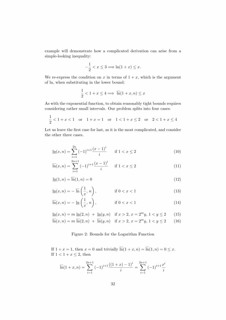
example will demonstrate how a complicated derivation can arise from asimple-looking inequality:

−1

2< x ≤ 3 =⇒ ln(1 + x) ≤ x.

We re-express the condition on x in terms of 1 + x, which is the argumentof ln, when substituting in the lower bound:

1

2< 1 + x ≤ 4 =⇒ ln(1 + x, n) ≤ x

As with the exponential function, to obtain reasonably tight bounds requiresconsidering rather small intervals. Our problem splits into four cases:

1

2< 1 + x < 1 or 1 + x = 1 or 1 < 1 + x ≤ 2 or 2 < 1 + x ≤ 4

Let us leave the first case for last, as it is the most complicated, and considerthe other three cases.

ln(x, n) =2n∑

i=1

(−1)i+1 (x− 1)i

iif 1 < x ≤ 2 (10)

ln(x, n) =2n+1∑

i=1

(−1)i+1 (x− 1)i

iif 1 < x ≤ 2 (11)

ln(1, n) = ln(1, n) = 0 (12)

ln(x, n) = − ln

(

1

x, n

)

, if 0 < x < 1 (13)

ln(x, n) = − ln

(

1

x, n

)

, if 0 < x < 1 (14)

ln(x, n) = m ln(2, n) + ln(y, n) if x > 2, x = 2my, 1 < y ≤ 2 (15)

ln(x, n) = m ln(2, n) + ln(y, n) if x > 2, x = 2my, 1 < y ≤ 2 (16)

Figure 2: Bounds for the Logarithm Function

If 1 + x = 1, then x = 0 and trivially ln(1 + x, n) = ln(1, n) = 0 ≤ x.If 1 < 1 + x ≤ 2, then

ln(1 + x, n) =2n+1∑

i=1

(−1)i+1 ((1 + x)− 1)i

i=

2n+1∑

i=1

(−1)i+1xi

i

32

by equation (11). Setting n = 0 yields ln(1 + x, n) = x and reduces ourinequality to the trivial x ≤ x.

If 2 < 1 + x ≤ 4, then we have to apply equation (16). That requiresfinding a positive integer m and some y such that 1+x = 2my and 1 < y ≤ 2.Clearly m = 1. In this case, putting n = 0, we have

2n+1∑

i=1

(−1)i+1 (2− 1)i

i+

2n+1∑

i=1

(−1)i+1 (y − 1)i

i= 1 + (y − 1)

= y

≤ 2y − 1

= x.

Now, let us turn to that postponed first case. If 12 < 1 + x < 1, then

1 < 1/(1 + x) < 2. Putting n = 1, we have

ln(1 + x, n) = − ln

(

1

1 + x, n

)

= −2n∑

i=1

(−1)i+1( 1

1+x − 1)i

i

=

2n∑

i=1

(−1)i

i

(

−x

1 + x

)i

=

(

x

1 + x

)

+

(

1

2

)(

−x

1 + x

)2

.

Now(

x

1 + x

)

+

(

1

2

)(

−x

1 + x

)2

≤ x ⇐⇒

x(1 + x) +1

2x2 ≤ x(1 + x)2 ⇐⇒

x+3

2x2 ≤ x+ 2x2 + x3 ⇐⇒

−1

2x2 ≤ x3 ⇐⇒

−1

2≤ x

which holds because 12 < 1+x. Note that putting n = 0 would have required

us to prove 0 ≤ x, which fails.This derivation reveals some limitations. We should have been able

to prove this result with looser bounds on x, since ln(1 + x) ≤ x holds forx > −1. We could not do this because our upper bound, ln(x, n), introducesthe value m in equation (16). This formulation allows the upper bound to

33

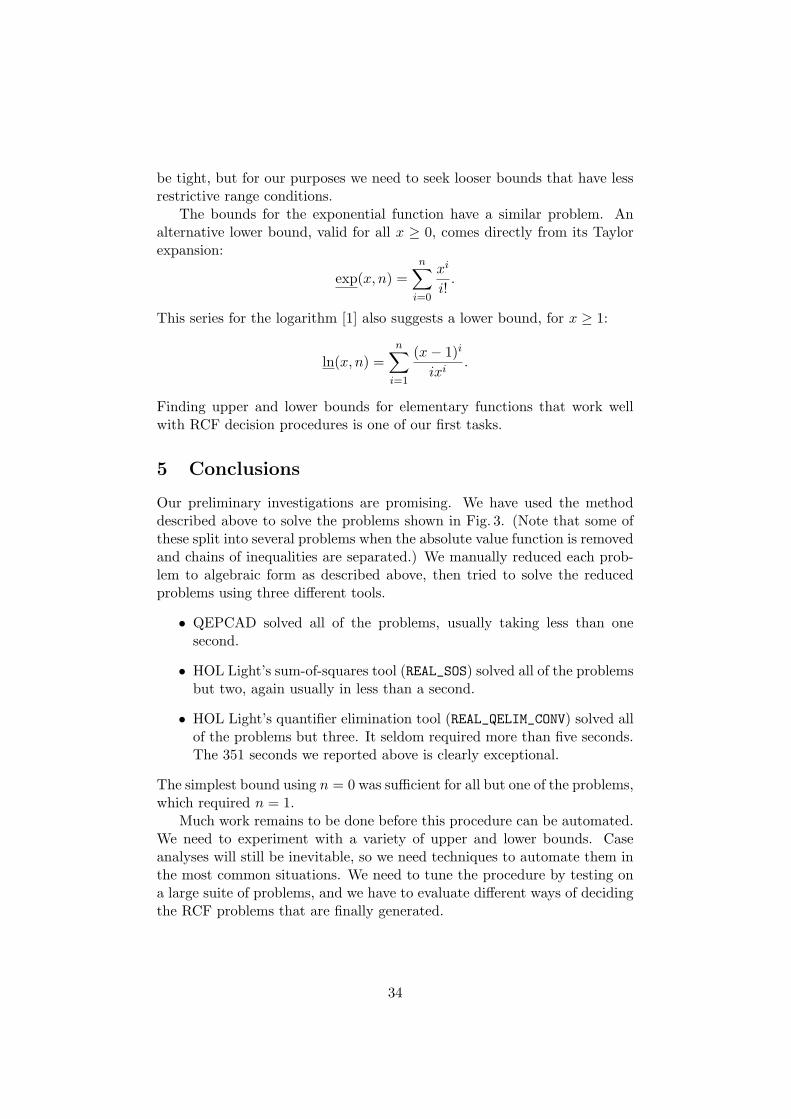
be tight, but for our purposes we need to seek looser bounds that have lessrestrictive range conditions.

The bounds for the exponential function have a similar problem. Analternative lower bound, valid for all x ≥ 0, comes directly from its Taylorexpansion:

exp(x, n) =

n∑

i=0

xi

i!.

This series for the logarithm [1] also suggests a lower bound, for x ≥ 1:

ln(x, n) =n∑

i=1

(x− 1)i

ixi.

Finding upper and lower bounds for elementary functions that work wellwith RCF decision procedures is one of our first tasks.

5 Conclusions

Our preliminary investigations are promising. We have used the methoddescribed above to solve the problems shown in Fig. 3. (Note that some ofthese split into several problems when the absolute value function is removedand chains of inequalities are separated.) We manually reduced each prob-lem to algebraic form as described above, then tried to solve the reducedproblems using three different tools.

• QEPCAD solved all of the problems, usually taking less than onesecond.

• HOL Light’s sum-of-squares tool (REAL_SOS) solved all of the problemsbut two, again usually in less than a second.

• HOL Light’s quantifier elimination tool (REAL_QELIM_CONV) solved allof the problems but three. It seldom required more than five seconds.The 351 seconds we reported above is clearly exceptional.

The simplest bound using n = 0 was sufficient for all but one of the problems,which required n = 1.

Much work remains to be done before this procedure can be automated.We need to experiment with a variety of upper and lower bounds. Caseanalyses will still be inevitable, so we need techniques to automate them inthe most common situations. We need to tune the procedure by testing ona large suite of problems, and we have to evaluate different ways of decidingthe RCF problems that are finally generated.

34

−1

2≤ x ≤ 3 =⇒

x

1 + x≤ ln(1 + x) ≤ x

−3 ≤ x ≤1

2=⇒

−x

1− x≤ ln(1− x) ≤ −x

0 ≤ x ≤ 3 =⇒ |ln(1 + x)− x| ≤ x2

−3 ≤ x ≤ 0 =⇒ |ln(1− x) + x| ≤ x2

|x| ≤1

2=⇒ |ln(1 + x)− x| ≤ 2x2

|x| ≤1

2=⇒ |ln(1− x) + x| ≤ 2x2

0 ≤ x ≤ 0.5828 =⇒ |ln(1− x)| ≤3x

2

−0.5828 ≤ x ≤ 0 =⇒ |ln(1 + x)| ≤ −3x

21

2≤ x ≤ 4 =⇒ lnx ≤ x− 1

0 ≤ x ≤ 1 =⇒ e(x−x2) ≤ 1 + x

−1 ≤ x ≤ 1 =⇒ 1 + x ≤ ex

−1 ≤ x ≤ 1 =⇒ 1− x ≤ e−x

−1 ≤ x ≤ 1 =⇒ ex ≤1

1− x

−1 ≤ x ≤ 1 =⇒ e−x ≤1

1 + x

x ≤1

2=⇒ e−x/(1−x) ≤ 1− x

−1

2≤ x =⇒ ex/(1+x) ≤ 1 + x

0 ≤ x ≤ 1 =⇒ e−x ≤ 1−x

2

−1 ≤ x ≤ 0 =⇒ ex ≤ 1 +x

2

0 ≤ |x| ≤ 1 =⇒1

4|x| ≤ |ex − 1| ≤

7

4|x|

Figure 3: Problems Solved

35

Acknowledgements

The research was funded by the epsrc grant EP/C013409/1, Beyond Lin-ear Arithmetic: Automatic Proof Procedures for the Reals. R. W. Butler,D. Lester, J. Harrison and C. Munoz answered many questions. A. Chaieband the referees commented on this paper.

References

[1] M. Abramowitz and I. A. Stegun. Handbook of Mathematical Functionswith Formulas, Graphs, and Mathematical Tables. Wiley, 1972.

[2] J. Avigad, K. Donnelly, D. Gray, and P. Raff. A formally verified proofof the prime number theorem. ACM Trans. Comput. Logic, in press.

[3] A. Dolzmann, T. Sturm, and V. Weispfenning. Real quantifier elim-ination in practice. Technical Report MIP-9720, Universitat Passau,D-94030, Germany, 1997.

[4] J. Harrison. A HOL theory of Euclidean space. In Hurd and Melham[7], pages 114–129.

[5] H. Hong. QEPCAD — quantifier elimination by partial cylin-drical algebraic decomposition. Available on the Internet athttp://www.cs.usna.edu/~qepcad/B/QEPCAD.html.

[6] W. A. Hunt, Jr., R. B. Krug, and J. Moore. Linear and nonlineararithmetic in ACL2. In D. Geist and E. Tronci, editors, Correct Hard-ware Design and Verification Methods (CHARME), LNCS 2860, pages319–333, 2003.

[7] J. Hurd and T. Melham, editors. Theorem Proving in Higher OrderLogics: TPHOLs 2005, LNCS 3603. Springer, 2005.

[8] S. McLaughlin and J. Harrison. A proof-producing decision procedurefor real arithmetic. In R. Nieuwenhuis, editor, Automated Deduction— CADE-20 International Conference, LNAI 3632, pages 295–314.Springer, 2005.

[9] C. Munoz and D. Lester. Real number calculations and theorem prov-ing. In Hurd and Melham [7], pages 195–210.

[10] P. A. Parrilo. Semidefinite programming relaxations for semialgebraicproblems. Mathematical Programming, 96(2):293–320, 2003.

[11] D. Richardson. Some undecidable problems involving elementary func-tions of a real variable. Journal of Symbolic Logic, 33(4):514–520, Dec.1968.

36

[12] A. Tiwari. Abstraction based theorem proving: An example from thetheory of reals. In C. Tinelli and S. Ranise, editors, PDPAR: Workshopon Pragmatics of Decision Procedures in Automated Deduction, pages40–52. INRIA, Nancy, 2003.

37

Rewrite-Based Satisfiability Procedures for

Recursive Data Structures

Maria Paola Bonacina and Mnacho Echenim

Dipartimento di InformaticaUniversita degli Studi di Verona, Italy

Abstract

If a rewrite-based inference system is guaranteed to terminate onthe axioms of a theory T and any set of ground literals, then anytheorem-proving strategy based on that inference system is a rewrite-based decision procedure for T -satisfiability. In this paper, we considerthe class of theories defining recursive data structures, that might ap-pear out of reach for this approach, because they are defined by aninfinite set of axioms. We overcome this obstacle by designing a prob-lem reduction that allows us to prove a general termination result forall these theories. We also show that the theorem-proving strategy de-cides satisfiability problems in any combination of these theories withother theories decided by the rewrite-based approach.

1 Introduction

Most state-of-the-art verification tools rely on built-in satisfiability proce-dures for specific theories. These satisfiability procedures can be quite com-plicated to design and combine, and significant effort is devoted to provingthem correct and complete, and implementing them. A new approach todefining satisfiability procedures was introduced in [3], where the authorsshowed that a sound and complete first-order theorem-proving strategy canbe used to solve satisfiability problems for several theories of data structures.The idea behind this approach is that since such a strategy is a semi-decisionprocedure for first-order validity, if one proves that it terminates on a pre-sentation of the theory of interest T and any set of ground literals, thenit is a decision procedure for T -satisfiability. In [3], this idea was appliedto a standard inference system, the superposition calculus SP , and severaltheories, including those of arrays and possibly cyclic lists.

Since most verification problems involve more than one theory, a signif-icant advantage of an approach based on generic reasoning is that it makesit conceptually simple to combine theories, by considering the union of theirpresentations. Along with several experimental results that showed the prac-ticality of the rewrite-based approach, the authors of [1] defined the notion

38

of variable-inactive theories. This variable-inactivity condition guaranteesthat SP terminates on a combination of theories, provided it terminates oneach individual theory. The authors showed that an SP-based strategy is asatisfiability procedure for any combination of the theories of [3] and thosethey considered.

Several of the theories for which SP has been shown to yield satisfiabilityprocedures involve lists. The superposition calculus yields satisfiability pro-cedures for the theories of lists a la Shostak and a la Nelson and Oppen (see[3]), and for the theory of lists with nil (see [2]). A theory of lists that wasnot yet considered is that of acyclic lists, where formulae such as car(x) ' xare unsatisfiable. This theory, along with that of integer offsets consideredin [6, 1], belong to the general class of theories of recursive data structures,that we denote RDS. Each member of this class is denoted RDSk, wherek represents the number of selectors in the theory. We shall see that thetheory of integer offsets is RDS1, and the theory of acyclic lists is RDS2.In this paper, we investigate how a rewrite-based inference system can beused to solve any RDSk-satisfiability problem, for any k. The contributionsof the paper are the following:

• Every theory in the classRDS is presented by an infinite set of axioms,which cannot be given as an input to a theorem prover. Here, wepresent a reduction that conquers this infinite presentation problem.

• We prove that for any fair search plan, the inference system terminateson any reduced RDSk-satisfiability problem.

• We show that for every k, the theory RDSk can be combined with allthe theories considered in [3, 1, 2], namely those of lists a la Shostakand a la Nelson and Oppen, arrays and records with or without ex-tensionality, sets with extensionality, possibly empty lists and integeroffsets modulo.

Related work. Theories of recursive data structures were studied by Op-pen in [8], where he described a linear satisfiability procedure for the casewhere uninterpreted function symbols are excluded. In [9], Zhang et al.investigated quantifier-elimination problems for an extension of the theoryconsidered by Oppen: their setting includes atoms (constants) and severaldifferent constructors. However, their setting also excludes uninterpretedfunction symbols. They provided a satisfiability procedure for this theorythat “guesses” a so-called type completion, to determine which constructorwas used on each term, or whether the term is an atom, and then callsOppen’s algorithm.

In this paper, we consider the recursive data structures as defined in [8],since our aim was to investigate how to apply the rewrite-based method-ology to theories defined by infinite sets of axioms. Similar to any other

39

theory for which the superposition calculus can be used as a satisfiabilityprocedure, all these theories can be combined with the theory of equalitywith uninterpreted functions. For instance, it can be used to prove theRDSk-unsatisfiability of a set such as

S = cons(c1, . . . , ck) ' c, cons(c1, . . . , ck) ' c′, f(c) 6' f(c′),

where f is an uninterpreted function symbol.Due to space restrictions, the proofs were not included in this paper.

They can all be found in [5].

Preliminaries

In the following, given a signature Σ, we consider the standard definitionsof Σ-terms, Σ-literals and Σ-theories. The symbol ' denotes unorderedequality, and ./ is either ' or 6'. Unless stated otherwise, the letters xand y will denote variables, d and e elements of an interpretation domain,and all other lower-case letters will be constants or function symbols in Σ.Given a term t, Var(t) denotes the set of variables appearing in t. If t is aconstant or a variable, then the depth of t is depth(t) = 0, and otherwise,depth(f(t1, . . . , tn)) = 1 + maxdepth(ti) | i = 1, . . . , n. The depth of aliteral is defined by depth(l ./ r) = depth(l) + depth(r). A positive literal isflat if its depth is 0 or 1, and a negative literal is flat if its depth is 0. Wewill make use of the following standard result: given a signature Σ and aΣ-theory T , let S be a finite set of Σ-literals. Then there exists a signatureΣ′ obtained from Σ by adding a finite number of constants, and a finite setS′ of flat Σ′-literals such that S′ is T -satisfiable if and only if S is.

A simplification ordering  is an ordering that is stable, monotonic andcontains the subterm ordering : if s  t, then c[s]σ  c[t]σ for any contextc and substitution σ, and if t is a subterm of s then s  t. A completesimplification ordering, or CSO, is a simplification ordering that is totalon ground terms. We write t ≺ s if and only if s  t. More details onorderings can be found, e.g., in [4]. A CSO is extended to literals andclauses by multiset extension as usual, and when no confusion is possible,we will mention maximal literals without any reference to Â.

The superposition calculus, or SP , is a rewrite-based inference systemwhich is refutationally complete for first-order logic with equality (see, e.g.,[7]). It consists of expansion and contraction rules, and is based on a CSOon terms which is extended to literals and clauses in a standard way. Givena CSO Â, we write SPÂ for SP with Â. An SPÂ-derivation is a sequence

S0 `SPÂ S1 `SPÂ . . . Si `SPÂ . . . ,

each Si being a set of clauses obtained by applying an expansion or a con-traction rule to clauses in Si−1. Such a derivation yields a set of persistent

40

clauses :S∞ =

⋃

j≥0

⋂

i≥j

Si,

which can of course be infinite. Given a finite set of ground literals S, inorder to prove that the set of persistent clauses obtained by a fair SPÂ-derivation from T ∪S is finite, we may impose additional restrictions on theCSO Â. Any CSO verifying these restrictions will be termed as T -good. Wealso say that an SPÂ-strategy is T -good if the CSO Â is T -good.

A clause C is variable-inactive for  if no maximal literal in C is anequation t ' x, where x /∈ Var(t). A set of clauses is variable-inactive for if all its clauses are variable-inactive for Â. A theory presentation Tis variable-inactive for  if the limit S∞ of any fair SPÂ-derivation fromS0 = T ∪ S is variable-inactive. When no confusion is possible, we will saythat a clause (resp. a set of clauses or a theory presentation) is variable-inactive, without any mention of Â.

2 The theory of recursive data structures

The theory RDSk of recursive data structures is based on the followingsignature:

ΣRDSk = cons ∪ Σsel ,

Σsel = sel1, . . . , selk,

where cons has arity k, and the seli’s all have arity 1. The function symbolssel1, . . . , selk stand for the selectors, and cons stands for the constructor.This theory is axiomatized by the following (infinite) set of axioms, denotedAx(RDSk):

seli(cons(x1, . . . , xi, . . . , xk)) ' xi for i = 1, . . . , k

cons(sel1(x), . . . , selk(x)) ' x,

t[x] 6' x,

where x and the xi’s are (implicitly) universally quantified variables and t[x]is any compound Σsel -term where the variable x occurs. The axioms t[x] 6' xare acyclicity axioms that prevent the theory from entailing equations suchas sel1(sel2(sel3(x))) ' x.

For the sake of clarity, we also define

Ac = t[x] 6' x | t[x] is a Σsel -term,

Ac[n] = t[x] 6' x | t[x] is a Σsel -term and depth(t[x]) ≤ n.

41

Example 1 Consider the case where k = 2. If we write car(x) instead ofsel1(x) and cdr(x) instead of sel2(x), then our axioms become:

car(cons(x, y)) ' x,

cdr(cons(x, y)) ' y,

cons(car(x), cdr(x)) ' x,

t[x] 6' x,

and for example, we have:

Ac[2] = car(car(x)) 6' x, cdr(cdr(x)) 6' x,car(cdr(x)) 6' x, cdr(car(x)) 6' x.

We consider the problem of checking the RDSk-satisfiability of a set Sof ground (equational) literals built out of the symbols in ΣRDSk and a setof finitely many constant symbols. This is done by checking the satisfiabilityof the following set of clauses:

Ax(RDSk) ∪ S.

According to the methodology of [3, 1, 2], this problem is solved in threephases:

Flattening: flatten all ground literals in the original problem, thus obtain-ing an equisatisfiable set of flat literals,

RDSk-reduction: transform the flattened problem into an equisatisfiableRDSk-reduced problem consisting of a finite set of clauses,

Termination: prove that any fair SPÂ-strategy terminates on the RDSk-reduced problems.

The flattening step is straightforward, and we now focus on the RDSk-reduction step.

3 RDSk-reduction

The aim of a reduction is to transform a formula into another one which isequisatisfiable and easier to work on. Here, given a formula S, we want totransform it into a formula which is equisatisfiable in a theory that does notaxiomatize the relationship between the constructor and the selectors. Webegin by observing that S can be transformed by suppressing either everyoccurrence of cons, or every occurrence of the seli’s.

42

Example 2 Consider the case where k = 2, and let

S = cons(c1, c2) ' c, sel1(c) ' c′1.

If we remove the occurrence of cons, S would become

S1 = sel1(c) ' c1, sel2(c) ' c2, sel1(c) ' c′1.

If we remove the occurrence of sel1, S would become

S2 = cons(c1, c2) ' c, c1 ' c′1.

We choose to remove every occurrence of cons because it is easier to workwith function symbols of arity 1:

Definition 3 A set of ground flat literals is RDSk-reduced if it contains nooccurrence of cons. 3

Given a set S of ground flat literals, the symbol cons may appear only inliterals of the form cons(c1, . . . , ck) ' c for constants c, c1, . . . , ck. Negativeground flat literals are of the form c 6' c′ and therefore do not containany occurrence of cons. The RDSk-reduction of S is obtained by replacingevery literal cons(c1, . . . , ck) ' c appearing in S by the literals sel1(c) 'c1, . . . , selk(c) ' ck. The resulting RDSk-reduced form S′ of S is denotedRedRDSk(S), and it is obviously unique.

It is not intuitive in which theory the RDSk-reduced form of S is equi-satisfiable to S, and we need the following definition:

Definition 4 Let (ext) denote the following “extensionality lemma”:

k∧

i=1

(selk(x) ' selk(y)) ⇒ x ' y. 3

Proposition 5 The extensionality lemma is logically entailed by the axiomcons(sel1(x), . . . , selk(x)) ' x.

We can then show that RDSk-reduction reduces satisfiability w.r.t.Ax(RDSk) to satisfiability w.r.t. Ac ∪ (ext).

Lemma 6 Let S be a set of ground flat literals, then Ax(RDSk) ∪ S issatisfiable if and only if Ac ∪ (ext) ∪ RedRDSk(S) is.

The first implication of this lemma is quite simple to prove, we show onan example the idea behind the proof of the converse implication.

43

Example 7 Consider the case where k = 1 and S = cons(c′) ' c, theRDS1-reduced form of S is therefore S′ = sel1(c) ' c′. We consider themodel M = (N, I) of Ac∪(ext)∪S′, where I interprets c as 0, c′ as 1, andsel1 as the successor function on natural numbers. We construct a modelM ′ = (D′, I ′) of Ax(RDS1) ∪ S, such that D ⊆ D′ and I ′ is identical to Ion D, as follows.

Intuitively, since M ′ must satisfy the axiom cons(sel1(x)) ' x, I ′ willinterpret cons as the predecessor function. Hence, for every d ∈ N \ 0,cons

I′(d) is the predecessor of d.However, the predecessor function on natural numbers is not defined

for 0. In order to define correctly the value of consI′(0), we augment D

with a new element, say −1, and obtain a new set D1. Then we definecons

I′(0) = −1, and selI′

1 (−1) = 0. We now need to define the value ofcons

I′(−1), so we augment D1 with a new element, say −2, and definecons

I′(−1) = −2, and selI′

1 (−2) = −1.By iterating this process, we obtain the model M ′ = (D′, I ′), where

D′ = Z, I ′ interprets sel1 as the standard successor function on integers,and cons as the standard predecessor function on integers. It is clear thatM ′ is a model of Ax(RDS1) ∪ S.

It is also possible to define a notion of RDSk-reduction where every oc-currence of the seli’s is removed. However, no additional property is gainedby using this other alternative, and the corresponding reduction is less in-tuitive.

4 From Ac to Ac[n]

The set Ac being infinite, SP cannot be used as a satisfiability procedureon any set of the form Ac ∪ (ext) ∪ S. Thus, the next move is to boundthe number of axioms in Ac needed to solve the satisfiability problem, andtry to consider an Ac[n] instead of Ac. It is clear that for any n and anyset S, a model of Ac ∪ (ext) ∪ S is also a model of Ac[n] ∪ (ext) ∪ S,the difficulty is therefore to determine an n for which a model of Ac ∪ S isguaranteed to exist, provided Ac[n]∪(ext)∪S is satisfiable. The followingexample provides the intuition that this bound depends on the number ofselectors in S.

Example 8 Let S = sel1(c1) ' c2, sel2(c2) ' c3, sel3(c3) ' c4, c1 ' c4.Then:

Ac[1] ∪ (ext) ∪ S and Ac[2] ∪ (ext) ∪ S are satisfiable,Ac[3] ∪ (ext) ∪ S and Ac ∪ (ext) ∪ S are unsatisfiable.

The following lemma allows us prove that having n occurrences of selec-tors implies that it is indeed sufficient to consider Ac[n] instead of Ac.

44

Lemma 9 Let S be an RDSk-reduced set of ground flat literals and let lbe the number of occurrences of selectors in S. For n ≥ l, suppose thatAc[n] ∪ (ext) ∪ S is satisfiable. Then Ac[n+ 1] ∪ (ext) ∪ S is alsosatisfiable.

A simple induction using Lemma 9 shows that for every k ≥ 0, if Ac[n]∪Sis satisfiable, then so is Ac[n+ k] ∪ S. We can therefore deduce:

Corollary 10 Let S be an RDSk-reduced set of ground flat literals and letn be the number of occurrences of selectors in S. Then, Ac ∪ (ext) ∪ S issatisfiable if and only if Ac[n] ∪ (ext) ∪ S is.

5 SPÂ as a satisfiability procedure

We now show that only a finite number of clauses are generated by thesuperposition calculus on any set Ac[n] ∪ (ext) ∪ S, where S is RDSk-reduced. This will be the case provided we use an RDSk-good CSO:

Definition 11 A CSO  is RDSk-good if t  c for every ground compoundterm t and every constant c. 3

Lemma 12 Let S0 = Ac[n]∪(ext)∪S, where S is a finite RDSk-reducedset of ground flat literals. Consider the limit S∞ of the derivation S0 `SPÂS1 `SPÂ . . . generated by a fair RDSk-good SPÂ-strategy; every clause inS∞ belongs to one of the categories enumerated below:

i) the empty clause;

ii) the clauses in Ac[n] ∪ (ext), i.e.

a) t[x] 6' x, where t is a Σsel -term of depth at most n,

b) x ' y ∨

(

∨ki=1

(seli(x) 6' seli(y))

)

;

iii) ground clauses of the form

a) c ' c′ ∨ (∨mj=1

dj 6' d′j) where m ≥ 0,

b) f(c) ' c′ ∨ (∨mj=1

dj 6' d′j) where m ≥ 0,

c) t[c] 6' c′ ∨ (∨mj=1

dj 6' d′j), where t is a compound Σsel -term ofdepth at most n− 1 and m ≥ 0,

d)∨mj=1

dj 6' d′j, where m ≥ 1;

iv) clauses of the form

c ' x ∨

(

∨jp=1

selip(c) 6' selip(x)

)

∨

(

∨kp=j+1

cip 6' selip(x)

)

∨(

∨mj=1

dj 6' d′j

)

45

where i1, . . . , ik is a permutation of 1, . . . , k, 0 ≤ j ≤ k and m ≥ 0;

v) clauses of the form

c ' c′ ∨

(

∨j1p=1

(selip(c) 6' selip(c′))

)

∨

(

∨j2p=j1+1

(selip(c) 6' c′ip

)

)

∨(

∨j3p=j2+1

(cip 6' selip(c′))

)

∨

(

∨kp=j3+1

(cip 6' c′ip

)

)

∨(

∨mj=1

dj 6' d′j

)

where i1, . . . , ik is a permutation of 1, . . . , k, 0 ≤ j1 ≤ j2 ≤ j3 ≤ k,j3 > 0 and m ≥ 0.

This lemma is proved by induction on the length l of the derivations.The result is true for l = 0: the clauses in S0 are in (ii) or (iii) with m = 0.A case analysis shows that if the result is true for l − 1, then it is also truefor l. We give an example of such a derivation:

Example 13 Consider the case where k = 3, and suppose we want to testthe unsatisfiability of the following set:

S = sel1(c) ' d1, sel2(c′) ' d′2, sel2(c) ' d2,sel1(c′) ' d′1, sel3(c) ' d3, sel3(c′) ' d′3,

d1 ' d′1, d2 ' d′2, d3 ' d′3,c 6' c′ .

• A superposition of sel1(c) ' d1 into (ext) yields a clause in (iv)(with m = 0):

c ' x ∨(

sel2(c) 6' sel2(x) ∨ sel3(c) 6' sel3(x))

∨(

d1 6' sel1(x))

,

• A superposition of sel2(c′) ' d′2 into the underlined literal of this clauseyields a clause in (v):

c ' c′ ∨(

sel3(c) 6' sel3(c′))

∨(

sel2(c) 6' d′2

)

∨(

d1 6' sel1(c′))

,

• A simplification of this clause by sel2(c) ' d2 yields a clause in (v):

c ' c′ ∨(

sel3(c) 6' sel3(c′))

∨(

d1 6' sel1(c′))

∨(

d2 6' d′2

)

,

• Further simplifications by sel1(c′) ' d′1, sel3(c) ' d3 and sel3(c′) ' d′3yield the clause

c ' c′ ∨

( 3∨

i=1

di 6' d′i

)

.

46

• The simplifications by di ' d′i for i = 1, . . . , 3 yield the clause c ' c′,which together with c 6' c′ produces the empty clause.

Since the signature is finite, there are finitely many clauses such as thoseenumerated in Lemma 12. We therefore deduce:

Corollary 14 Any fair RDSk-good SPÂ-strategy terminates when appliedto Ac[n] ∪ (ext) ∪ S, where S is a finite RDSk-reduced set of ground flatliterals.

We can also evaluate the complexity of this procedure by determiningthe number of clauses in each of the categories defined in Lemma 12.

Theorem 15 Any fair RDSk-good SPÂ-strategy is an exponential satisfi-ability procedure for RDSk.

Proof. Let n be the number of literals in S, both the number of constantsand the number of selectors appearing in S are therefore in O(n). Weexamine the cardinalities of each of the categories defined in Lemma 12.

• Category (ii) contains O(n) clauses if k = 1 and O(kn) clauses if k ≥ 2.

• Clauses in categories (iii), (iv) or (v) can contain any literal of theform d 6' d′ where d and d′ are constants, thus, these categories allcontain O(2n

2

) clauses.

Hence, the total number of clauses generated is bound by a constant whichis O(2n

2

), and since each inference step is polynomial, the overall procedureis in O(2n

2

).

Although this complexity bound is exponential, it measures the size ofthe saturated set. Since a theorem prover seeks to generate a proof, asopposed to a saturated set, the relevance of this result with respect to pre-dicting the performance of a theorem prover can therefore be quite limited.

One could actually have expected this procedure to be exponential fork ≥ 2, since in that case Ac[n] contains an exponential number of axioms.However the procedure is also exponential when k = 1, and a more care-ful analysis shows that this complexity is a consequence of the presence of(ext). In fact, it was shown in [2] that any fair SPÂ-strategy is a polyno-mial satisfiability procedure for the theory presented by the set of acyclicityaxioms Ac when k = 1.

We finally address combination by proving that RDSk is variable-inactive for SPÂ.

Theorem 16 Let S0 = Ac[n] ∪ S ∪ (ext), where S is an RDSk-reducedset of ground flat literals, and n is the number of occurrences of selectors inS. Then S∞ is variable-inactive.

47

Proof. The clauses in S∞ belong to one of the classes enumerated inLemma 12. Thus, the only clauses of S∞ that may contain a literal t ' xwhere x /∈ Var(t) are in class (iv). Since  is a CSO, the literals t ' xcannot be maximal in those clauses.

This shows that the rewrite-based approach to satisfiability procedurescan be applied to the combination of RDSk with any number of the theoriesconsidered in [3, 1], including those of arrays and records with or withoutextensionality.

6 Conclusion

In this paper, we considered a class of theories representing recursive datastructures, each of which is defined by an infinite set of axioms. We showedthat the superposition calculus can be used as the basis of a satisfiabilityprocedure for any theory in this class, and this result was obtained by defin-ing a reduction that permits to restrict the number of acyclicity axioms tobe taken into account.

A main issue we plan to investigate is complexity, since the basic pro-cedure is exponential. A linear algorithm for such structures was obtainedin [8], but it excludes uninterpreted function symbols. The setting of [6]includes uninterpreted function symbols, but the authors gave a polynomialalgorithm only for the case where k = 1 (the theory of integer offsets). Weintend to investigate making the complexity of the rewrite-based proceduredependent on k, and improving the bound for k = 1.

From the point of view of practical efficiency, we plan to test the per-formance of a state-of-the-art theorem prover on problems featuring thistheory, possibly combined with those of [3, 1], and compare it with systemsimplementing decision procedures from other approaches. In this context,we may work on designing specialized search plans for satisfiability prob-lems. Another direction for future work is to examine how the rewrite-based approach applies to recursive data structures with an atom predicate,or multiple constructors.

Acknowledgments

The authors wish to thank Silvio Ranise for bringing this class of theoriesto their attention and for his encouragement.

References

[1] Alessandro Armando, Maria Paola Bonacina, Silvio Ranise, and StephanSchulz. On a rewriting approach to satisfiability procedures: Extension,combination of theories and an experimental appraisal. In Bernhard

48

Gramlich, editor, Frontiers of Combining Systems, 5th InternationalWorkshop, FroCoS 2005, Vienna, Austria, September 19-21, 2005, Pro-ceedings, volume 3717 of Lecture Notes in Computer Science, pages 65–80. Springer, 2005.

[2] Alessandro Armando, Maria Paola Bonacina, Silvio Ranise, and StephanSchulz. On a rewriting approach to satisfiability procedures: Theoriesof data structures, modularity and experimental appraisal. TechnicalReport RR 36/2005, Dipartimento di Informatica, Universita degli Studidi Verona, 2006.

[3] Alessandro Armando, Silvio Ranise, and Michael Rusinowitch. A rewrit-ing approach to satisfiability procedures. Inf. Comput., 183(2):140–164,2003.

[4] Franz Baader and Tobias Nipkow. Term Rewriting and All That. Cam-bridge University Press, 1998.

[5] Maria Paola Bonacina and Mnacho Echenim. Generic theorem prov-ing for decision procedures. Technical report, Universita degli studi diVerona, 2006. Available at http:profs.sci.univr.it/~echenim/.

[6] Robert Nieuwenhuis and Albert Oliveras. Congruence closure with inte-ger offsets. In Moshe Y. Vardi and Andrei Voronkov, editors, Logic forProgramming, Artificial Intelligence, and Reasoning, 10th InternationalConference, LPAR 2003, Almaty, Kazakhstan, September 22-26, 2003,Proceedings, volume 2850 of Lecture Notes in Computer Science, pages78–90. Springer, 2003.

[7] Robert Nieuwenhuis and Albert Rubio. Paramodulation-based theoremproving. In John Alan Robinson and Andrei Voronkov, editors, Handbookof Automated Reasoning, pages 371–443. Elsevier and MIT Press, 2001.

[8] Derek C. Oppen. Reasoning about recursively defined data structures.J. ACM, 27(3):403–411, 1980.

[9] Ting Zhang, Henny B. Sipma, and Zohar Manna. Decision proceduresfor recursive data structures with integer constraints. In David A. Basinand Michael Rusinowitch, editors, Automated Reasoning - Second Inter-national Joint Conference, IJCAR 2004, Cork, Ireland, July 4-8, 2004,Proceedings, volume 3097 of Lecture Notes in Computer Science, pages152–167. Springer, 2004.

49

An Abstract Decision Procedure for Satisfiability in the

Theory of Recursive Data Types

Clark Barrett1 Igor Shikanian1 Cesare Tinelli2

1New York University, barrett|igor@cs.nyu.edu2The University of Iowa, tinelli@cs.uiowa.edu

Abstract

The theory of recursive data types is a valuable modeling tool for software verifica-tion. In the past, decision procedures have been proposed for both the full theory andits universal fragment. However, previous work has been limited in various ways. Inthis paper, we present a general algorithm for the universal fragment. The algorithmis presented declaratively as a set of abstract rules which are terminating, sound, andcomplete. We show how other algorithms can be realized as strategies within ourgeneral framework. Finally, we propose a new strategy and give experimental resultsshowing that it performs well in practice.

1 Introduction

Recursive data types are commonly used in programming. The same notion is also aconvenient abstraction for common data types such as records and data structures suchas linked lists used in more conventional programming languages. The ability to reasonautomatically and efficiently about recursive data types thus provides an important toolfor the analysis and verification of programs.

Perhaps the best-known example of a simple recursive data type is the list type used inLISP. Lists are either the null list or are constructed from other lists using the constructor

cons. This constructor takes two arguments and returns the result of prepending its firstargument to the list in its second argument. In order to retrieve the elements of a list, apair of selectors is provided: car returns the first element of a list and cdr returns the restof the list.

More generally, we are interested in any set of (possibly mutually) recursive data types,each of which contains one or more constructors. Each constructor has selectors that canbe used to retrieve the original arguments as well as a tester which indicates whether agiven term was constructed using that constructor. As an example of the more generalcase, suppose we want to model lists of trees of natural numbers. Consider a set of threerecursive data types: nat, list, and tree. nat has two constructors: zero, which takes noarguments (we call such a constructor a nullary constructor or constant); and succ, whichtakes a single argument of type nat and has the corresponding selector pred. The list typeis as before except that we now specify that the elements of the list are of type tree. Thetree type in turn has two constructors: node, which takes an argument of type list andhas the corresponding selector children, and leaf, which takes an argument of type nat andhas the corresponding selector data. We can represent this set of types using the followingconvenient notation based on that used in functional programming languages:

50

nat := succ(pred : nat) | zero;list := cons(car : tree, cdr : list) | null;tree := node(children : list) | leaf(data : nat);

The testers for this set of data types are is succ, is zero, is cons, is null, is node, andis leaf.

Propositions about a set of recursive data types can be captured in a sorted first-order language which closely resembles the structure of the data types themselves in thatit has function symbols for each constructor and selector, and a predicate symbol foreach tester. For instance, propositions that we would expect to be true for the exampleabove include: (i) ∀x : nat. succ(x) 6= zero; (ii) ∀x : list. x = null ∨ is cons(x); and (iii)∀x : tree. is leaf(x)→ (data(x) = zero ∨ is succ(data(x))).

In this paper, we discuss a procedure for deciding such formulas. We focus on satis-fiability of a set of literals, which (through well-known reductions) can be used to decidethe validity of universal formulas.

There are three main contributions of this work over earlier work on the topic. First,our setting is more general: we allow mutually recursive types and multiple constructors.The second contribution is in presentation. We present the theory itself in terms of aninitial model rather than axiomatically as is often done. Also, the presentation of thedecision procedure is given as abstract rewrite rules, making it more flexible and easier toanalyze than if it were given imperatively. Finally, as described in Section 4, the flexibilityprovided by the abstract algorithm allows us to describe a new strategy with significantlyimproved practical efficiency.

Related Work. Term algebras over constructors provide the natural intended modelfor recursive data types. In [7] two dual axiomatizations of term algebras are presented,one with constructors only, the other with selectors and testers only.

An often-cited reference for the quantifier-free case is the treatment by Nelson andOppen in 1980[11, 12] (where the problem is also shown to be NP-complete). In particular,Oppen’s algorithm in [12] gives a detailed decision procedure for a single recursive datatype with a single constructor; however, the case of multiple constructors is discussed onlybriefly and not rigorously.

More recently, several papers by Zhang et al. [14, 15] explore decision procedures for asingle recursive data type. These papers focus on ambitious schemes for quantifier elimina-tion and combinations with other theories. A possible extension of Oppen’s algorithm tothe case of multiple constructors is discussed briefly in [14]. A comparison of our algorithmwith that of [14] is made in Section 4.

Finally, another approach based on first-order reasoning with the superposition calculusis described in [5]. This work shows how a decision procedure for a recursive data type canbe automatically inferred from the first-order axioms, even though the axiomatization isinfinite. Although the results are impressive from a theoretical point of view, the scope islimited to theories with a single constructor and the practical efficiency of such a schemehas yet to be shown.

2 The Theory of Recursive Data Types

Previous work on recursive data types (RDTs) uses first-order axiomatizations in an at-tempt to capture the main properties of a recursive data type and reason about it. Wefind it simpler and cleaner to use a semantic approach instead, as is done in algebraic

51

specification. A set of RDTs can be given a simple equational specification over a suitablesignature. The intended model for our theory can be formally, and uniquely, defined asthe initial model of this specification. Reasoning about a set of RDTs then amounts toreasoning about formulas that are true in this particular initial model.

2.1 Specifying RDTs

We formalize RDTs in the context of many-sorted equational logic (see [9] among others).We will assume that the reader is familiar with the basic notions in this logic, and alsowith basic notions of term rewriting.

We start with the theory signature. We assume a many-sorted signature Σ whose setof sorts consists of a distinguished sort bool for the Booleans, and p ≥ 1 sorts τ1, . . . , τpfor the RDTs. We also allow r ≥ 0 additional (non-RDT) sorts σ1, . . . , σr. We will denoteby s, possibly with subscripts and superscripts, any sort in the signature other than bool,and by σ any sort in σ1, . . . , σr.

As mentioned earlier, the function symbols in our theory signature correspond to theconstructors, selectors, and testers of the set of RDTs under consideration. We assumefor each τi (1 ≤ i ≤ p) a set of mi ≥ 1 constructors of τi. We denote these symbols as Cij ,

where j ranges from 1 to mi. We denote the arity of Cij as nij (0-arity constructors are also

called nullary constructors or constants) and its sort as sij,1 × · · · × sij,nij→ τi. For each

constructor Cij , we have a set of selectors, which we denote as Sij,k, where k ranges from 1

to nij , of sort τi → sij,k. Finally, for each constructor, there is a tester1 isCij : τi → bool.In addition to these symbols, we also assume that the signature contains two constants,

true and false of sort bool, and an infinite number of distinct constants of each sort σ. Theconstants are meant to be names for the elements of that sort, so for instance if σ1 werea sort for the natural numbers, we could use all the numerals as the constants of sort σ1.Having all these constants in the signature is not necessary for our approach, but in thefollowing exposition it provides an easy way of ensuring that the sorts in σ are infinite.Section 5.1 shows that our approach can be easily extended to the case in which someof these sorts are finite. To summarize, the set of function symbols of the signature Σconsists of:

Cij : sij,1 × · · · × sij,nij→ τi, for i = 1, . . . , p, j = 1, . . . ,mi,

Sij,k : τi → sij,k, for i = 1, . . . , p, j = 1, . . . ,mi, k = 1, . . . , nij ,

isCij : τi → bool, for i = 1, . . . , p, j = 1, . . . ,mi,true : bool, false : bool,An infinite number of constants for each σl, for l = 1, . . . , r.

As usual in many-sorted equational logic, we also have p+ r+ 1 equality symbols (one foreach sort mentioned above), all written as ≈.

Our procedure requires one additional constraint on the set of RDTs: It must be well-

founded. Informally, this means that each sort must contain terms that are not cyclic orinfinite. More formally, we have the following definitions by simultaneous induction overconstructors and sorts: (i) a constructor Cij is well-founded if all of its argument sorts arewell-founded; (ii) the sorts σ1, . . . , σr are all well-founded; (iii) a sort τi is well-founded ifat least one of its constructors is well-founded. We require that every sort be well-foundedaccording to the above definition.

1To simplify some of the proofs, and without loss of generality, we use functions to bool instead ofpredicates for the testers.

52

In some cases, it will be necessary to distinguish between finite and infinite τ -sorts: (i)a constructor is finite if it is nullary or if all of its argument sorts are finite; (ii) a sort τi isfinite if all of its constructors are finite, and is infinite otherwise; (iii) the sorts σ1, . . . , σrare all infinite. As we will see, consistent with the above terminology, our semantics willinterpret finite, resp. infinite, τ -sorts indeed as finite, resp. infinite, sets.

We denote by T (Σ) the set of well-sorted ground terms of signature Σ or, equivalently,the (many-sorted) term algebra over that signature. The RDTs with functions and pred-icates denoted by the symbols of Σ are specified by the following set E of (universallyquantified) equations. For reasons explained below, we assume that associated with everyselector Sij,k : τi → sij,k is a distinguished ground term of sort sij,k containing no selectors

(or testers), which we denote by tij,k.

Equational Specification of the RDT: for i = 1, . . . , p:

∀x1, . . . , xnij. isCij(C

ij(x1, . . . , xnij

)) ≈ true (for j = 1, . . . ,mi)

∀x1, . . . , xnij′. isCij(C

ij′(x1, . . . , xni

j′)) ≈ false (for j, j′ = 1, . . . ,mi, j 6= j′)

∀x1, . . . , xnij. Sij,k(C

ij(x1, . . . , xnij

)) ≈ xk (for k = 1, . . . , nij , j = 1, . . . ,mi)

∀x1, . . . , xnij′. Sij,k(C

ij′(x1, . . . , xni

j′)) ≈ tij,k (for j, j′ = 1, . . . ,mi, j 6= j′)

The last axiom specifies what happens when a selector is applied to the “wrong”constructor. Note that there is no obviously correct thing to do in this case since it wouldcorrespond to an error condition in a real application. Our axiom specifies that in thiscase, the result is the designated ground term for that selector. This is different from othertreatments (such as [7, 14, 15]) where the application of a wrong selector is treated as theidentity function. The main reason for this difference is that identity function would notalways be well-sorted in multi-sorted logic.

By standard results in universal algebra we know that E admits an initial model R andwe can show the following result:2 Let Ω be the signature obtained from Σ by removingthe selectors and the testers; then, the reduct of R to Ω is isomorphic to T (Ω). Informally,this means that R does in fact capture the set of RDTs in question, as we can take thecarrier of R to be the term algebra T (Ω).

3 The Decision Procedure

In this section, we present a decision procedure for the satisfiability of sets of literalsover R. Our procedure builds on the algorithm by Oppen [12] for a single type witha single constructor. As an example of Oppen’s algorithm, consider the list data typewithout the null constructor and the following set of literals: cons(x, y) ≈ z, car(w) ≈x, cdr(w) ≈ y, w 6≈ z. Oppen’s algorithm uses a graph which relates terms accordingto their meaning in the intended model. Thus, cons(x, y) is a parent of x and y andcar(w) and cdr(w) are children of w. The equations induce an equivalence relation on thenodes of the graph. The Oppen algorithm proceeds by performing upwards (congruence)and downwards (unification) closure on the graph and then checking for cycles3 or for aviolation of any disequalities. For our example, upwards closure results in the conclusionw ≈ z, which contradicts the disequality w 6≈ z.

2Proofs of all results in this paper can be found in [4].3A simple example of a cycle is: cdr(x) ≈ x.

53

As another example, consider the following set of literals: cons(x, y) ≈ z, car(w) ≈x, cdr(w) ≈ y, v ≈ w, y 6≈ cdr(v). The new graph has a node for v, with cdr(v) asits right child. The Oppen algorithm requires that every node with at least one childhave a complete set of children, so car(v) is added as a left child of v. Now, downwardsclosure forces car(v) ≈ car(w) ≈ x and cdr(v) ≈ cdr(w) ≈ y, contradicting the disequalityy 6≈ cdr(v).

An alternative algorithm for the case of a single constructor is to introduce new termsand variables to replace variables that are inside of selectors. For example, for the first setof literals above, we would introduce w ≈ cons(s, t) where s, t are new variables. Now, bysubstituting and collapsing applications of selectors to constructors, we get cons(x, y) ≈z, w ≈ cons(s, t), x ≈ s, t ≈ y, w 6≈ z. In general, this approach only requires downwardsclosure.

Unfortunately, with the addition of more than one constructor, things are not quite assimple. In particular, the simple approach of replacing variables with constructor termsdoes not work because one cannot establish a priori whether the value denoted by agiven variable is built with one constructor or another. A simple extension of Oppen’salgorithm for the case of multiple constructors is proposed in [14]. The idea is to firstguess a type completion, that is, a labeling of every variable by a constructor, which ismeant to constrain a variable to take only values built with the associated constructor.Once all variables are labeled by a single constructor, the Oppen algorithm can be used todetermine if the constraints can be satisfied under that labeling. Unfortunately, the typecompletion guess can be very expensive in practice.

Our presentation combines ideas from all of these algorithms as well as introducingsome new ones. There is a set of upward and downward closure rules to mimic Oppen’salgorithm. The idea of a type completion is replaced by a set of labeling rules that canbe used to refine the set of possible constructors for each term (in particular, this allowsus to delay guessing as long as possible). And the notion of introducing constructors andeliminating selectors is captured by a set of selector rules. In addition to the presentation,one of our key contributions is to provide precise side-conditions for when case splitting isnecessary as opposed to when it can be delayed. The results given in Section 4 show thatwith the right strategy, significant gains in efficiency can be obtained.

We describe our procedure formally in the following, as a set of derivation rules. Webuild on and adopt the style of similar rules for abstract congruence closure [1] and syn-tactic unification [8].

3.1 Definitions and Notation

In the following, we will consider well-sorted formulas over the signature Σ above and aninfinite set X of variables. To distinguish these variables, which can occur in formulasgiven to the decision procedure described below, from other internal variables used by thedecision procedure, we will sometimes call the elements of X input variables.

Given a set Γ of literals over Σ and variables from X, we wish to determine thesatisfiability of Γ in the algebra R. We will assume for simplicity, and with no lossof generality, that the only occurrences of terms of sort bool are in atoms of the formisCjk(t) ≈ true, which we will write just as isCjk(t).

Following [1], we will make use of the sets Vτi (Vσi) of abstraction variables of sort τi(σi); abstraction variables are disjoint from input variables (variables in Γ) and functionas equivalence class representatives for the terms in Γ. We assume an arbitrary, but fixed,well-founded ordering  on the abstraction variables that is total on variables of the same

54

sort. We denote the set of all variables (both input and abstraction) in E as Var(E). Wewill use the expression lbls(τi) for the set Ci

1, . . . , Cimi and define lbls(σl) to be the empty

set of labels for each σl. We will write sort(t) to denote the sort of the term t.The rules make use of three additional constructs that are not in the language of Σ:

→, 7→, and Inst.The symbol → is used to represent oriented equations. Its left-hand side is a Σ-term

t and its right-hand side is an abstraction variable v. The symbol 7→ denotes labellings ofabstraction variables with sets of constructor symbols. It is used to keep track of possibleconstructors for instantiating a τi variable.4 Finally, the Inst construct is used to trackapplications of the Instantiate rules given below. It is needed to ensure termination bypreventing multiple applications of the same Instantiate rule. It is a unary predicatethat is applied only to abstraction variables.

Let ΣC denote the set of all constant symbols in Σ, including nullary constructors. Wewill denote by Λ the set of all possible literals over Σ and input variables X. Note thatthis does not include oriented equations (t→ v), labeling pairs (v 7→ L), or applications ofInst. In contrast, we will denote by E multisets of literals of Λ, oriented equations, labelingpairs, and applications of Inst. To simplify the presentation, we will consistently use thefollowing meta-variables: c, d denote constants (elements of ΣC) or input variables fromX; u, v, w denote abstraction variables; t denotes a flat term—i.e., a term all of whoseproper sub-terms are abstraction variables—or a label set, depending on the context.u,v denote possibly empty sequences of abstraction variables; and u → v is shorthandfor the set of oriented equations resulting from pairing corresponding elements from u

and v and orienting them so that the left hand variable is greater than the right handvariable according to Â. Finally, v ./ t denotes any of v ≈ t, t ≈ v, v 6≈ t, t 6≈ v, orv 7→ t. To streamline the notation, we will sometimes denote function application simplyby juxtaposition.

Each rule consists of a premise and one or more conclusions. Each premise is madeup of a multiset of literals, oriented equations, labeling pairs, and applications of Inst.Conclusions are either similar multisets or ⊥, where ⊥ represents a trivially unsatisfiableformula. The soundness of our rule-based procedure depends on the fact that the premiseE of a rule is satisfied in R by a valuation α of Var(E) iff one of the conclusions E′ of therule is satisfied in R by an extension of α to Var(E′).

3.2 The derivation rules

Our decision procedure consists of the following derivation rules on multisets E.

Abstraction rules

Abstract 1p[c], E

c→ v, v 7→ lbls(s), p[v], Eif

p ∈ Λ, c : s,v fresh from Vs

Abstract 2p[Ciju], E

Ciju→ v, p[v], v 7→ Cij, Eif p ∈ Λ, v fresh from Vτi

Abstract 3

p[Sij,ku], E

Sij,1u→ v1, . . . , Sij,nij

u→ vnij, p[vk],

v1 7→ lbls(s1), . . . , vnij7→ lbls(snij

), E

ifp ∈ Λ, Sij,k : τi → sk,

each vι fresh from Vsι

4To simplify the writing of the rules, some rules may introduce labeling pairs for variables with a non-τsort, even though these play no role.

55

The abstraction or flattening rules assign a new abstraction variable to every sub-term in the original set of literals. Abstraction variables are then used as place-holdersor equivalence class representatives for those sub-terms. While we would not expect apractical implementation to actually introduce these variables, it greatly simplifies thepresentation of the remaining rules. Notice that in each case, a labeling pair for theintroduced variables is also created. This corresponds to labeling each sub-term with theset of possible constructors with which it could have been constructed. Also notice thatin the Abstract 3 rule, whenever a selector Sij,k is applied, we effectively introduce allpossible applications of selectors associated with the same constructor. This simplifies thelater selector rules and corresponds to the step in the Oppen algorithm which ensures thatin the term graph, any node with children has a complete set of children.

Literal level rules

Orientu ≈ v, E

u→ v, Eif u  v

Inconsistentv 6≈ v, E

⊥

Remove 1isCij v, E

v 7→ Cij, E

Remove 2¬isCij v, E

v 7→ lbls(sort(v)) \ Cij, E

The simple literal level rules are mostly self-explanatory. The Orient rule is used toreplace an equation between abstraction variables (which every equation eventually be-comes after applying the abstraction rules) with an oriented equation. Oriented equationsare used in the remaining rules below. The Remove rules remove applications of testersand replace them with labeling pairs that impose the same constraints.

Upward (i.e., congruence) closure rules

Simplify 1u ./ t, u→ v, E

v ./ t, u→ v, E

Simplify 2fuuv→ w, u→ v, E

fuvv→ w, u→ v, E

Superposet→ u, t→ v, E

u→ v, t→ v, Eif u  v

Composet→ v, v → w, E

t→ w, v → w, E

These rules are modeled after similar rules for abstract congruence closure in [1]. TheSimplify and Compose rules essentially provide a way to replace any abstraction variablewith a smaller (according to Â) one if the two are known to be equal. The Superpose

rule merges two equivalence classes if they contain the same term. Congruence closure isachieved by these rules because if two terms are congruent, then after repeated applicationsof the first set of rules, they will become syntactically identical. Then the Superpose rulewill merge their two equivalence classes.

Downward (i.e., unification) closure rules

DecomposeCiju→ v, Cijv→ v, E

Ciju→ v, u→ v, E

Clashc→ v, d→ v, E

⊥if c, d ∈ ΣC, c : σ, d : σ, c 6= d

56

CycleCinjnunuvn→un−1, . . . , C

i2j2

u2u2v2→u1, Ci1j1

u1u1v1→u,E

⊥if n ≥ 1

The main downward closure rule is the Decompose rule: whenever two terms withthe same constructor are in the same equivalence class, their arguments must be equal.The Clash rule detects instances of terms that are in the same equivalence class thatmust be disequal in the intended model. The Cycle rule detects the (inconsistent) casesin which a term would have to be cyclical.

Selector rules

Instantiate 1Sij,1u→ u1, . . . , S

ij,nij

u→ unij, u 7→ Cij, E

Ciju1 · · ·unij→ u, u 7→ Cij, Inst(u), E

if Inst(u) 6∈ E

Instantiate 2

v 7→ Cij, E

Ciju1 · · ·unij→ v, Inst(v), E

u1 7→ lbls(sij,1), . . . , unij7→ lbls(si

j,nij)

if

Inst(v) 6∈ E,v 7→ L 6∈ E,Cij finite constructor,

Sab,c(v)→ v′ 6∈ E,

uk fresh from Vsij,k

Collapse 1Ciju1 · · ·unij

→ u, Sij,ku→ v, E

Ciju1 · · ·unij→ u, uk ≈ v, E

Collapse 2Sij,ku→ v, u 7→ L, E

tij,k ≈ v, u 7→ L, Eif Cij /∈ L

Rule Instantiate 1 is used to eliminate selectors by replacing the argument of theselectors with a new term constructed using the appropriate constructor. Notice thatonly terms that have selectors applied to them can be instantiated and then only oncethey are unambiguously labeled. Rule Instantiate 2 is used for finite constructors. Forcompleteness, terms labeled with finite constructors must be instantiated even when noselectors are applied to them. The Collapse rules eliminate selectors when the result oftheir application can be determined. In Collapse 1, a selector is applied to a term knownto be equal to a constructor of the “right” type. In this case, the selector expression isreplaced by the appropriate argument of the constructor. In Collapse 2, a selector isapplied to a term which must have been constructed with the “wrong” constructor. Inthis case, the designated term tij,k for the selector replaces the selector expression.

Labeling rules

Refinev 7→ L1, v 7→ L2, E

v 7→ L1 ∩ L2, EEmpty

v 7→ ∅, E

⊥if v : τi

Split 1Sij,k(u)→ v, u 7→ Cij ∪ L, E

Sij,k(u)→ v, u 7→ Cij, E Sij,k(u)→ v, u 7→ L, Eif L 6= ∅

Split 2u 7→ Cij ∪ L, E

u 7→ Cij, E u 7→ L, Eif

L 6= ∅,Cij ∪ L all finite constructors

57

The Refine rule simply combines labeling constraints that may arise from differentsources for the same equivalence class. Empty enforces the constraint that every τ -termmust be constructed by some constructor. The splitting rules are used to refine the setof possible constructors for a term and are the only rules that cause branching. If a termlabeled with only finite constructors cannot be eliminated in some other way, Split 2 mustbe applied until it is labeled unambiguously. For other terms, the Split 1 rule only needsto be applied to distinguish the case of a selector being applied to the “right” constructorfrom a selector being applied to the “wrong” constructor. On either branch, one of theCollapse rules will apply immediately. We discuss this further in Section 4, below. Therules are proved sound, complete and terminating in our full report [4].

4 Strategies and Efficiency

It is not difficult to see that the problem of determining the satisfiability of an arbitraryset of literals is NP-complete. The problem was shown to be NP-hard in [12]. To seethat it is in NP, we note that given a type completion, no additional splits are necessary,and the remaining rules can be carried out in polynomial time. However, as with otherNP-complete problems (Boolean satisfiability being the most obvious example), the rightstrategy can make a significant difference in practical efficiency.

4.1 Strategies

A strategy is a predetermined methodology for applying the rules. Before discussing ourrecommended strategy, it is instructive to look at the closest related work. Oppen’s originalalgorithm is roughly equivalent to the following: After abstraction, apply the selector rulesto eliminate all instances of selector symbols. Next, apply upward and downward closurerules (the bidirectional closure). As you go, check for conflicts using the rules that canderive ⊥. We will call this the basic strategy. Note that it excludes the splitting rules:because Oppen’s algorithm assumes a single constructor, the splitting rules are never used.A generalization of Oppen’s algorithm is mentioned in [14]. They add the step of initiallyguessing a “type completion”. To model this, consider the following simple Split rule:

Splitu 7→ Cij ∪ L, E

u 7→ Cij, E u 7→ L, Eif L 6= ∅

Now consider a strategy which invokes Split greedily (after abstraction) until it no longerapplies and then follows the basic strategy. We will call this strategy the greedy splitting

strategy. One of the key contributions of this paper is to recognize that the greedy splittingstrategy can be improved in two significant ways. First, the simple Split rule should bereplaced with the smarter Split 1 and Split 2 rules. Second, these rules should be delayedas long as possible. We call this the lazy splitting strategy. The lazy strategy reduces thesize of the resulting derivation in two ways. First, notice that Split 1 is only enabled whensome selector is applied to u. By itself, this eliminates many needless case splits. Second,by applying the splitting rules lazily (in particular by first applying selector rules), it maybe possible to avoid splitting completely in many cases.

Example. Consider the following simple tree data type: tree := node(left : tree, right :tree) | leaf with leaf as the designated term for both selectors. Suppose we receive theinput formula leftn(Z) ≈ X ∧ is node(Z) ∧ Z ≈ X. After applying all available rulesexcept for the splitting rules, the result will look something like this:

58

Worst Case Greedy LazyNumber of Splits Benchmarks Sat Unsat Splits Time (s) Splits Time (s)

0 4416 306 4110 0 24.6 0 24.6

1-5 2520 2216 304 6887 16.8 2414 17.0

6-10 692 571 121 4967 5.8 1597 5.7

11-20 178 112 66 2422 2.3 517 1.6

21-100 145 73 72 6326 4.5 334 1.1

101+ 49 11 38 16593 9.8 73 0.3

Table 1: Greedy vs. Lazy Splitting

Z → u0, X → u0, u0 7→ node,node(u1, v1)→ u0, un → u0,left(u1)→ u2, . . . , left(un−1)→ un, u1 7→ leaf,node, . . . , un 7→ leaf,node,right(u1)→v2,. . ., right(un−1)→vn, v1 7→ leaf,node, . . . , vn 7→ leaf,node,

Notice that there are 2n abstraction variables labeled with two labels each. If we eagerlyapplied the naive Split rule at this point, the derivation tree would reach size O(22n).

Suppose, on the other hand, that we use the lazy strategy. First notice that Split

1 can only be applied to n of the abstraction variables (ui, 1 ≤ i ≤ n). Thus the morerestrictive side-conditions of Split 1 already reduce the size of the problem to at worstO(2n) instead of O(22n). However, by only applying it lazily, we do even better: supposewe split on ui. The result is two branches, one with ui 7→ node and the other withui 7→ leaf. The second branch induces a cascade of (at most n) applications of Collapse2 which in turn results in uk 7→ leaf for each k > i. This eventually results in ⊥ viathe Empty and Refine rules. The other branch contains ui 7→ node and results in theapplication of the Instantiate rule, but little else, and so we will have to split again, thistime on a different ui. This process will have to be repeated until we have split on all ofthe ui. At that point, there will be a cycle from u0 back to u0, and so we will derive ⊥ viathe Cycle rule. Because each split only requires at most O(n) rules and there are n − 1splits, the total size of the derivation tree will be O(n2).

4.2 Experimental Results

We have implemented both the lazy and the greedy splitting strategies in the theoremprover CVC Lite [2]. Using the mutually recursive data types nat, list, and tree mentionedin the introduction, we randomly generated 8000 benchmarks.5

As might be expected with a large random set, most of the benchmarks are quite easy.In fact, over half of them are solved without any case splitting at all. However, a fewof them did prove to be somewhat challenging (at least in terms of the number of splitsrequired). Table 1 shows the total time and case splits required to solve the benchmarks.The benchmarks are divided into categories based on the the maximum number of casesplits required to solve the benchmark.

For easy benchmarks that don’t require many splits, the two algorithms perform almostidentically. However, as the difficulty increases, the lazy strategy performs much better.For the hardest benchmarks, the lazy strategy outperforms the greedy strategy by morethan an order of magnitude.

5See http://www.cs.nyu.edu/~barrett/datatypes for details on the benchmarks and results.

59

5 Extending the Algorithm

In this section we briefly discuss several ways in which our algorithm can be used as acomponent in solving a larger or related problem.

5.1 Finite Sorts

Here we consider how to lift the limitation imposed before that each of σ ∈ σ1, . . . , σr isinfinite valued. Since we have no such restrictions on sorts τi, the idea is to simply replacesuch a σ by a new τ -like sort τσ, whose set of constructors (all of which will be nullary)will match the domain of σ. For example, if σ is a finite scalar of the form 1, . . . , n,then we can let τσ ::== null1 | . . . | nulln. We then proceed as before, after replacing alloccurrences of σ by τσ and each i by nulli.

5.2 Simulating Partial Function Semantics

As mentioned earlier, it is not clear how best to interpret the application of a selector to thewrong constructor. One compelling approach is to interpret selectors as partial functions.An evaluation of a formula then has three possible outcomes: true, false, or undefined.This approach may be especially valuable in a verification application in which applicationof selectors is required to be guarded so that no formula should ever be undefined. Thiscan easily be implemented by employing the techniques described in [6]: given a formula tocheck, a special additional formula called a type-correctness condition is computed (whichcan be done in time and space linear in the size of the input formula). These two formulascan then be checked using a decision procedure that interprets the partial functions (inthis case, the selectors) in some arbitrary way over the undefined part of the domain. Theresult can then be interpreted to reveal whether the formula would have been true, false,or undefined under the partial function semantics.

5.3 Cooperating with other Decision Procedures

A final point is that that our procedure has been designed to integrate easily into a Nelson-Oppen-style framework for cooperating decision procedures [10]. In the many-sorted case,the key theoretical requirements (see [13]) for two decision procedures to be combinedare that the signatures of their theories share at most sort symbols and each theory isstably infinite over the shared sorts.6 A key operational requirement is that the decisionprocedure is also able to easily compute and communicate equality information.

The theory of R (i.e., the set of sentences true in R) is trivially stably infinite over thesorts σ1, . . . , σr and over any τ -sort containing a non-finite constructor—as all such sortsdenote infinite sets in R. Also, in our procedure the equality information is eventuallycompletely captured by the oriented equations produced by the derivation rules, and soentailed equalities can be easily detected and reported.

For a detailed and formal discussion of how to integrate a rule-based decision proceduresuch as this one into a general framework combining Boolean reasoning and multipledecision procedures, we refer the reader to our related work in [3]. Note that, in particular,this work shows how the internal theory case splits can be delegated on demand to theBoolean engine; this is the implementation strategy followed in CVC Lite.

6A many-sorted theory T is stably infinite over a subset S of its sorts if every quantifier-free formulasatisfiable in T is satisfiable in a model of T where the sorts of S denote infinite sets.

60

References

[1] L. Bachmair, A. Tiwari, and L. Vigneron. Abstract congruence closure. JAR, 31:129–168,2003.

[2] C. Barrett and S. Berezin. CVC Lite: A new implementation of the cooperating validitychecker. In Proceedings of CAV, pages 515–518, July 2004.

[3] C. Barrett, R. Nieuwenhuis, A. Oliveras, and C. Tinelli. Splitting on demand in sat-isfiability modulo theories. Technical report, University of Iowa, 2006. Available atftp://ftp.cs.uiowa.edu/pub/tinelli/papers/BarNOT-RR-06.pdf.

[4] C. Barrett, I. Shikanian, and C. Tinelli. An abstract decision procedure for satisfiability inthe theory of recursive data types. Technical Report TR2005-878, Department of ComputerScience, New York University, Nov. 2005.

[5] M. P. Bonacina and M. Echenim. Generic theorem proving for decision proce-dures. Technical report, Universita degli studi di Verona, 2006. Available athttp://profs.sci.univr.it/∼echenim/.

[6] S. B. et al. A practical approach to partial functions in CVC Lite. In W. A. et al., editor,Selected Papers from PDPAR ’04, volume 125(3) of ENTCS, pages 13–23. Elsevier, July 2005.

[7] W. Hodges. A Shorter Model Theory. Cambridge University Press, 1997.

[8] A. Martelli and U. Montanari. An efficient unification algorithm. ACM Transactions on

Programming Languages and Systems, 4(2):258–282, 1982.

[9] K. Meinke and J. V. Tucker. Universal algebra. In S. Abramsky, D. V. Gabbay, and T. S. E.Maibaum, editors, Handbook of Logic in Computer Science, volume 1. Claredon Press, 1992.

[10] G. Nelson and D. Oppen. Simplification by cooperating decision procedures. ACM Transac-

tions on Programming Languages and Systems, 1(2):245–57, 1979.

[11] G. Nelson and D. C. Oppen. Fast decision procedures based on congruence closure. JACM,27(2):356–364, April 1980.

[12] D. C. Oppen. Reasoning about recursively defined data structures. JACM, 27(3):403–411,July 1980.

[13] C. Tinelli and C. Zarba. Combining decision procedures for sorted theories. In J. Alferes andJ. Leite, editors, Proceedings of JELIA ’04, volume 3229 of LNAI, pages 641–653. Springer,2004.

[14] T. Zhang, H. B. Sipma, and Z. Manna. Decision procedures for term algebras with integerconstraints. In Proceedings of IJCAR ’04 LNCS 3097, pages 152–167, 2004.

[15] T. Zhang, H. B. Sipma, and Z. Manna. Term algebras with length function and boundedquantifier alternation. In Proceedings of TPHOLs, 2004.

61

A Framework for Decision Procedures in

Program Verification(presentation-only paper)

Ofer Strichman1 and Daniel Kroening2

1 Technion, Haifa, Israel2 ETH Zurich, Switzerland

ofers@ie.technion.ac.il, daniel.kroening@inf.ethz.ch

Abstract

Program analysis tools for modern programming languages requirea very rich logic to reason about constructs such as bit-vector oper-ators or dynamic data structures. We propose a generic frameworkfor reducing decidable decision problems to propositional logic thatstarts with an axiomatization of the logics. Instantiating the frame-work for a specific logic requires a deductive decision procedure thatfulfills several conditions. Linear arithmetic, the theory of arrays andother logics useful for verification, have such a decision procedure, aswe show. Further, the framework allows to reduce combined theoriesto a unified propositional formula, which enables learning across the-ories. We conclude by presenting several challenges that need to bemet for making the framework more general and useful for programverification.

62

Easy Parameterized Verificaton of

Biphase Mark and 8N1 Protocols(presentation-only paper)

Geoffrey Brown1 and Lee Pike 2

1 Indiana University2 Galois Connections

geobrown@cs.indiana.edu, leepike@galois.com

Abstract

The Biphase Mark Protocol (BMP) and 8N1 Protocol are physicallayer protocols for data transmission. We present a generic model inwhich timing and error values are parameterized by linear constraints,and then we use this model to verify these protocols. The verificationsare carried out using SRI’s SAL model checker that combines a sat-isfiability modulo theories decision procedure with a bounded modelchecker for highly-automated induction proofs of safety properties overinfinite-state systems. Previously, parameterized formal verification ofreal-time systems required mechanical theorem-proving or specializedreal-time model checkers; we describe a compelling case-study demon-strating a simpler and more general approach. The verification revealsa significant error in the parameter ranges for 8N1 given in a publishedapplication note.

63

Predicate Learning and Selective Theory

Deduction for Solving Difference Logic(presentation-only paper)

Chao Wang, Aarti Gupta, Malay Ganai

NEC Labs America, Princeton, USA

chaowang|agupta|malay@nec-labs.com

Abstract

Design and verification of systems at the Register-Transfer (RT) orbehavioral level require the ability to reason at higher levels of abstrac-tion. Difference logic consists of an arbitrary Boolean combination ofpropositional variables and difference predicates and therefore providesan appropriate abstraction. In this paper, we present several new op-timization techniques for efficiently deciding difference logic formulas.We use the lazy approach by combining a DPLL Boolean SAT proce-dure with a dedicated graph-based theory solver, which adds transitiv-ity constraints among difference predicates on a “need-to” basis. Ournew optimization techniques include flexible theory constraint prop-agation, selective theory deduction, and dynamic predicate learning.We have implemented these techniques in our lazy solver. We demon-strate the effectiveness of the proposed techniques on public bench-marks through a set of controlled experiments.

64

Deciding Extensions of the Theory of

Arrays by Integrating Decision

Procedures and Instantiation Strategies(presentation-only paper)

Silvio Ghilardi1, Enrica Nicolini1,

Silvio Ranise2 and Daniele Zucchelli1

1 Universita degli Studi di Milano, Italy2 LORIA and INRIA-Lorraine, Nancy, France

ghilardi@dsi.unimi.it, nicolini@mat.unimi.it,

silvio.ranise@loria.fr, zucchelli@dsi.unimi.it

Abstract

The theory of arrays, introduced by McCarthy in his seminal pa-per “Toward a mathematical science of computation”, is central toComputer Science. Unfortunately, the theory alone is not sufficientfor many important verification applications such as program analysis.Motivated by this observation, we study extensions of the theory ofarrays whose satisfiability problem (i.e. checking the satisfiability ofconjunctions of ground literals) is decidable. In particular, we considerextensions where the indexes of arrays has the algebraic structure ofPresburger Arithmetic and the theory of arrays is augmented with ax-ioms characterizing additional symbols such as dimension, sortedness,or the domain of definition of arrays.

We provide methods for integrating available decision proceduresfor the theory of arrays and Presburger Arithmetic with automatic in-stantiation strategies which allow us to reduce the satisfiability problemfor the extension of the theory of arrays to that of the theories decidedby the available procedures. Our approach aims to reuse as much aspossible existing techniques so to ease the implementation of the pro-posed methods. To this end, we show how to use both model-theoreticand rewriting-based theorem proving (i.e., superposition) techniquesto implement the instantiation strategies of the various extensions.

65

Producing Conflict Sets

for Combinations of Theories(presentation-only paper)

Silvio Ranise, Christophe Ringeissen and Duc-Khanh Tran

LORIA and INRIA-Lorraine, Nancy, France

ranise|ringeiss|tran@loria.fr

Abstract

Recently, it has become evident that the capability of computingconflict sets is of paramount importance for the efficiency of systems forSatisfiability Modulo Theories (SMT). In this paper, we consider theproblem of modularly constructing conflict sets for a combined theory,when this is obtained as the disjoint union of many component theoriesfor which satisfiability procedures capable of computing conflict setsare assumed available. The key idea of our solution to this problemis the concept of explanation graph, which is a labelled, acyclic andundirected graph capable of recording the entailment of some elemen-tary equalities. Explanation graphs allow us to record the explanationscomputed by, for instance, a proof-producing congruence closure andto extend the well-known Nelson-Oppen combination method to mod-ularly build conflict sets for disjoint unions of theories. We study howthe computed conflict sets relate to an appropriate notion of minimal-ity.

66