towards the integration of theory and practice in ...anderson/diss/bastonidiss.pdfuniversita degli...
TRANSCRIPT

UNIVERSITA DEGLI STUDI DI ROMA
“TOR VERGATA”
Facolta di Ingegneria
Dipartimento di Informatica, Sistemi, e Produzione
Towards the Integration of Theory and Practicein Multiprocessor Real-Time Scheduling
by
Andrea Bastoni
Ph.D. program in Computer Science and Automation Engineering
Course: XXIII
A.A. 2010/2011
Advisor: Dott. Marco Cesati
Co-Advisor: Prof. James H. Anderson
Coordinator: Prof. Daniel P. Bovet

Abstract
Nowadays, multicore and multiprocessor platforms are the standard computing plat-
forms for desktop and server systems. Manufacturers of traditionally uniprocessor
embedded systems are also shifting towards multicore platforms. This deeply in-
fluences the design of real-time systems, where timing constraints must be met.
In the industrial world, the design of such systems largely relies on porting well-
established uniprocessor real-time scheduling algorithms to multicore platforms,
and practical factors related to the implementation of real-time systems are actually
the main focus. Conversely, academic institutions mainly focus on the theoretical
properties of multicore scheduling algorithms and on the development of new mul-
ticore scheduling policies; practical issues that arise in the implementation of such
policies on real multicore systems are seldomly considered.
Questions related to which multicore real-time scheduling policies are better
suited to support real-world workloads on multicore platforms are still largely unan-
swered, and overhead- and implementation-related issues pertaining to newly devel-
oped multicore scheduling algorithms have been largely ignored. Particularly, prior
work on the practical viability of multiprocessor real-time scheduling algorithms
has only partially tackled the challenges of the effects of complex interaction among
cache memories. Furthermore, detailed runtime overheads and cache-related delays
affecting recently developed multicore real-time scheduling algorithms have never
been measured before within a real operating system, and their schedulability under
consideration of overheads has never been evaluated.
ii
iii
This dissertation adds to prior work on the practical viability of multicore and
multiprocessor scheduling algorithms by devising methodologies for empirically
approximating cache-related overheads on multicore platforms with complex cache
hierarchies. To bridge the gap between multiprocessor real-time scheduling theory
and practical implementations of scheduling algorithms, we further investigate the
practical merits of recently proposed multicore scheduling algorithms that specif-
ically target the impacts of cache-related delays. In the proposed evaluations, the
effects of measured kernel overheads and cache-related delays are explicitly ac-
counted for.

Never worry about theory as long as
the machinery does what it’s supposed to do.
(R. A. Heinlein)

Acknowledgments
My graduate school career and this dissertation would not have been possible with-
out the help and the support of many people.
I am profoundly indebted with my advisor Marco Cesati and with Daniel Bovet
for giving me the chance to enroll in the graduate school and for supporting me ever
since I started the Ph.D. program. It has been a pleasure and a privilege working
with them and learning from them. I am thankful to Marco and Daniele for the
freedom they have always left me in the choice of research topics, and, at the same
time, for the help and suggestions on how to pursue my research objectives. I would
like to thank them for the precious advices related to kernel programming issues and
for leading me to understand how to write proper kernel code. I also owe Marco and
Daniele the chances to challenge myself into several teaching activities, which have
helped fostering my knowledge and improving my relational skills.
I am particularly grateful to my co-advisor Jim Anderson. He has always made
me feel as one of his students during my stay at UNC, and I am very thankful to him
for the great experience (both at academic and personal levels) it has been working
with him, and with the students of the Real-Time Group. I am indebted with Jim for
his patience with my poor language skills, for fixing my repetitive errors, and for
teaching me how to write and how to improve my presentation skills. I have always
been amazed by the concern and care Jim shows towards his students, and, although
the confidence Jim posed on me was sometimes overwhelming, it has greatly helped
me in improving and making progress in all of my works. I am also thankful to him
v

vi
for sponsoring the trips to several conferences, which have helped creating a better
knowledge of the real-time community.
Thanks also go to MBDA, and, in particular, to Christian Di Biagio, for the
Ph.D. fellowship that sponsored my graduate school.
I would like to thank all my colleagues in the SPRG group and all the graduate
students that have shared with me these graduate school years. I am particularly
thankful to Emiliano Betti, Paolo Palana, Roberto Gioiosa, and Gianluca Grilli for
their ingenious ideas and their prompt support. During these years, I have received
many useful feedbacks and I have had many productive discussions with all the
friends of the “S4ALab,” and I would like to thank particularly Antonio Grillo,
Alessandro Lentini, Vittorio Ottaviani, Francesco Piermaria, Diego De Cao, and
Danilo Croce. Special thanks go to Antonio for the constructive discussions during
the writing of this dissertation, and to his wife Sonia, for bearing with us while we
were discussing.
This dissertation would not have been possible without the feedbacks, the “real-
time lunches,” and the help of all the colleagues of the Real-Time Group at UNC,
and particularly Bjorn Brandenburg, Christopher Kenna, Glenn Elliot, Cong Liu,
and Alex Mills. Of them, Bjorn deserves a very special thank, not only for the
cooperation when we co-authored papers, but also for his friendship, his construc-
tive criticism, his hard work and his never-ending support when the road before the
deadline was all but easy. Special thanks go to Nora, for bearing with me discussing
with Bjorn (not infrequently) in the middle of the night, and over many many din-
ners. I would like to thank them, and all the people that have changed my experience
in the US into a very special experience.
The Residenti-in-the-US and the SPRG-in-the-US deserve my gratitude for ex-
changing ideas and talking with friends in not-necessarily-the-same timezone. Thanks
Laura, Cecilia, Paolo, and Emiliano for hosting me and for contributing to spread
the idea that Italians always know someone. Many friends have contributed (in
several different ways) to this dissertation. I especially owe Giuseppe, Luigi, and

vii
Andrea for their support and their always interesting ideas.
I am profoundly grateful to my caring family that has always trusted and sup-
ported me, and to my sister for her always positive personality.
Above all, I am profoundly thankful to Dani, for her constant presence even
when we were not physically close, for her support during these years, for her infi-
nite patience during all the week-ends and nights I spent writing this dissertation. I
owe her more than what can be written in words.

Contents
List of Abbreviations xi
1 Introduction 11.1 Real-Time Systems . . . . . . . . . . . . . . . . . . . . . . . . . . 2
1.2 Motivation . . . . . . . . . . . . . . . . . . . . . . . . . . . . . . . 4
1.3 Contributions . . . . . . . . . . . . . . . . . . . . . . . . . . . . . 6
1.4 Organization . . . . . . . . . . . . . . . . . . . . . . . . . . . . . . 11
2 Background and Related Work 122.1 Real-Time System Model . . . . . . . . . . . . . . . . . . . . . . . 12
2.1.1 Task Model . . . . . . . . . . . . . . . . . . . . . . . . . . 13
2.1.2 Hard and Soft Real-Time Constraints . . . . . . . . . . . . 14
2.1.3 Resource Model . . . . . . . . . . . . . . . . . . . . . . . 15
2.2 Real-Time Scheduling . . . . . . . . . . . . . . . . . . . . . . . . 17
2.2.1 Uniprocessor Scheduling . . . . . . . . . . . . . . . . . . . 18
2.2.2 Multiprocessor Scheduling . . . . . . . . . . . . . . . . . . 19
2.2.3 Global, Partitioned, and Clustered EDF . . . . . . . . . . . 22
2.2.4 Semi-Partitioned Multiprocessor Algorithms . . . . . . . . 25
2.3 Operating System and Hardware Capabilities . . . . . . . . . . . . 26
2.3.1 Run Queues . . . . . . . . . . . . . . . . . . . . . . . . . . 27
2.3.2 Inter-Processor Interrupts (IPIs) . . . . . . . . . . . . . . . 27
viii

Contents ix
2.3.3 Timers and Time Resolution . . . . . . . . . . . . . . . . . 28
2.4 Kernel Overheads and Caches . . . . . . . . . . . . . . . . . . . . 28
2.5 Related Work . . . . . . . . . . . . . . . . . . . . . . . . . . . . . 31
2.5.1 Prior Work on Cache-Related Delays . . . . . . . . . . . . 31
2.5.2 Evaluation of Multiprocessor EDF Scheduling Algorithms . 34
2.5.3 Evaluation of Semi-Partitioned Algorithms . . . . . . . . . 35
3 Real-Time Operating Systems 373.1 OS Latency and Jitter . . . . . . . . . . . . . . . . . . . . . . . . . 37
3.2 Problems of Predictability in Linux . . . . . . . . . . . . . . . . . . 39
3.3 LITMUSRT . . . . . . . . . . . . . . . . . . . . . . . . . . . . . . 42
4 Semi-Partitioned Multiprocessor Scheduling Algorithms 474.1 EDF-fm . . . . . . . . . . . . . . . . . . . . . . . . . . . . . . . . 47
4.2 EDF-WM . . . . . . . . . . . . . . . . . . . . . . . . . . . . . . . 48
4.3 NPS-F . . . . . . . . . . . . . . . . . . . . . . . . . . . . . . . . 51
4.4 Implementation Concerns . . . . . . . . . . . . . . . . . . . . . . . 53
4.4.1 Timing Concerns . . . . . . . . . . . . . . . . . . . . . . . 53
4.4.2 Migration-related Concerns . . . . . . . . . . . . . . . . . 54
5 Measuring Overheads 555.1 Kernel Overheads . . . . . . . . . . . . . . . . . . . . . . . . . . . 56
5.1.1 Kernel Overheads under Multiprocessor EDF Algorithms . 57
5.1.2 Kernel Overheads under Semi-Partitioned Algorithms . . . 60
5.2 Cache-Related Delays . . . . . . . . . . . . . . . . . . . . . . . . . 61
5.2.1 Measuring Cache-Related Preemption and Migration Delays 63
5.2.2 Evaluation . . . . . . . . . . . . . . . . . . . . . . . . . . 68
6 Experimental Evaluation of Multiprocessor Scheduling Algorithms 796.1 Accounting for Overheads . . . . . . . . . . . . . . . . . . . . . . 80
Contents x
6.2 Schedulability Experiments . . . . . . . . . . . . . . . . . . . . . . 82
6.2.1 Task Set Generation . . . . . . . . . . . . . . . . . . . . . 82
6.2.2 Performance Metric . . . . . . . . . . . . . . . . . . . . . 83
6.3 Evaluation of Multiprocessor EDF Scheduling Algorithms . . . . . 86
6.4 Evaluation of Semi-Partitioned Algorithms . . . . . . . . . . . . . 95
6.4.1 NPS-F, C-NPS-F, and Choosing δ . . . . . . . . . . . . . 97
6.4.2 HRT and SRT Schedulability Results . . . . . . . . . . . . 99
6.4.3 Design Principles . . . . . . . . . . . . . . . . . . . . . . . 103
7 Conclusions 1067.1 Summary of Results . . . . . . . . . . . . . . . . . . . . . . . . . . 107
7.2 Future Work . . . . . . . . . . . . . . . . . . . . . . . . . . . . . . 109
A CPMD Data 111
B Overheads and Weighted Schedulability Resultsfor Multiprocessor EDF Scheduling Algorithms 116B.1 Measured Overheads . . . . . . . . . . . . . . . . . . . . . . . . . 116
B.2 Weighted Schedulability Results . . . . . . . . . . . . . . . . . . . 123
C Overheads and Weighted Schedulability Resultsfor Semi-partitioned Algorithms 137C.1 Measured Overheads . . . . . . . . . . . . . . . . . . . . . . . . . 137
C.2 Weighted Schedulability Results . . . . . . . . . . . . . . . . . . . 145
Bibliography 165
List of Abbreviations
C-EDF Clustered EDF
C-NPS-F Clustered variant of NPS-F
CPMD Cache-Related Preemption and Migration Delay
EDF Earliest Deadline First
EDF-fm EDF– Fixed/Migrating
EDF-WM EDF with Window-constraint Migration
FIFO First-In First-Out
G-EDF Global EDF
GPOS General Purpose Operating System
HRT Hard Real-Time
IRQ Interrupt ReQuest
LITMUSRT LInux Testbed for MUltiprocessor Scheduling in Real-
Time systems
NPS-F Notional Processor Scheduling – Fractional capacity
NUMA Non-Uniform Memory Access
OS Operating System
P-EDF Partitioned EDF
RM Rate Monotonic
RTOS Real-Time Operating System
xi

Contents xii
SRT Soft Real-Time
TSS Task Set Size
UMA Uniform Memory Access
WCET Worst-Case Execution Time
WS Working Set
WSS Working Set Size
Chapter 1
Introduction
The goal of this dissertation is to complement theoretical research on multiprocessor
real-time scheduling by measuring, evaluating and discussing the impact of practical
factors (such as implementation strategies and overheads) on multiprocessor real-
time scheduling algorithms. This work is motivated by the widespread diffusion of
multicore platforms as computing platforms for embedded, mobile, and ruggedized
real-time systems. Such systems were traditionally based on uniprocessor single-
board computers, where well-established uniprocessor real-time scheduling algo-
rithms could be employed. Instead, many scheduling-related theoretical results for
multiprocessor systems were obtained only recently. Furthermore, the optimiza-
tion of real-time performance on multicore systems poses new challenges, which
are specifically related to the effects of complex interaction among cache memo-
ries. Unfortunately, in theoretical work on multiprocessor and multicore real-time
scheduling algorithms, implementation-oriented issues and the impact of operating-
system and cache overheads have seldomly been considered. The work presented in
this thesis is therefore useful in order to evaluate how well the theoretical scheduling-
related properties of multiprocessor scheduling algorithms translate into practice
and which multiprocessor scheduling algorithms are better suited for different work-
loads.
1

1.1 Real-Time Systems 2
1.1 Real-Time Systems
Real-time systems are systems whose correctness depends not only on the results
of their computation, but also on the time at which the results are produced [43]. In
other words, real-time systems are subject to timing constraints. Examples of real-
time systems include automotive systems, command-and-control systems, radar sig-
nal processing and tracking systems, and air traffic control systems. Timing require-
ments are commonly characterized by deadlines, which specify the maximum time
an activity is allowed to complete its execution.
Real-time systems are not necessarily fast systems: the main objective of a fast
system is to minimize the average response time (i.e., the time interval from the
invocation of a task to its completion) of a set of tasks, while the objective of a real-
time system is to meet the timing requirements of each task. In a real-time system,
timing and functional requirements must be met under all possible circumstances,
and therefore, average response times and average performance provide little infor-
mation on the correct behavior of a real-time system. Instead, the most important
property of a real-time system is predictability [111]. Predictability means that it
should always be possible to prove that the behavior of the system will satisfy sys-
tem specifications. Nonetheless, a real-time system may be a fast system: for exam-
ple, a flight control real-time system must be able to quickly react to sudden changes
in the environment (e.g., crosswind gusts). The idea of time is strictly coupled with
the environment where the system operates. The environment is therefore an essen-
tial component of any real-time system, as it defines requirements and constraints
that must be met by the system.
Hard and soft real-time systems. Depending on the consequences that may oc-
cur because timing constraints are not satisfied, real-time systems are usually cat-
egorized in two classes: hard and soft. Hard real-time (HRT) systems are systems
where missing a deadline may cause catastrophic consequences: flight control sys-

1.1 Real-Time Systems 3
tems, automotive systems, and nuclear-plant control systems are example of hard
real-time systems. Instead, in soft real-time (SRT) systems, missing deadlines is
undesirable for performance reasons, but does not cause serious problems to the
environment and does not prevent the correct behavior of the system. Multimedia
applications are typical examples of soft real-time systems: a high-definition video
application playing a Blu-ray Disk must be able to process one video frame every
16ms for the playback to look “smooth” to the end user; missing deadlines in this
context only produces a degraded viewing experience.
Real-time operating systems. Once a real-time application’s functional-require-
ments and deadlines have been defined according to the constraints imposed by
the environment, the primary objective of a real-time operating system (RTOS) in
supporting the application is to ensure that hard real-time task deadlines will be
met [43, 85]. Soft real-time tasks and non-real-time tasks are commonly handled
using best-effort and heuristic strategies that attempt to reduce or minimize their
average response times.1 Clearly, real-time operating systems (as all operating sys-
tems) should also fulfill the objectives of interacting with the hardware components
of a system by abstracting applications from low-level platform details, and of mul-
tiplexing the execution of multiple applications in order to improve the utilization
of the hardware platform.
Since interacting with the environment is crucial in real-time systems, interrupt-
and time-management functionalities provided by real-time operating systems play
a fundamental role. Predictability of interrupt- and time-management routines (and
often fast response times and reduced latencies — see Ch. 3), as well as scheduling-
related functionalities, are among the most important features real-time operating
systems should provide. The critical role played by these routines can be seen in1Since the definition of “soft real-time systems” is not a clear-cut, several strategies may be adopted
in order to meet soft-real-time deadlines. As presented in Sec. 2.1.2, this thesis focuses on a schedule-centric definition of soft real-time where deadline tardiness is bounded. Under such definition, optimalSRT scheduling algorithms will be presented.

1.2 Motivation 4
“drive-by-wire” cars [97, 120] where, for instance, commands given to the steering
wheel are converted into a series of inputs to the car computer, which receives them
as external interrupts. Such interrupts are processed by the operating system and are
timely delivered to the real-time process that calculates how the wheels should turn
in order to achieve the desired direction change, in the context of the current road-
surface conditions. Furthermore, the road-surface conditions are monitored through
the aid of sensors that communicate with the system by triggering additional inter-
rupts. These interrupts should be serviced while performing other time-constrained
activities such as the precise control of fuel injection (i.e., to minimize fuel con-
sumption). Since the major focus of this thesis is on scheduling-related issues,
aspects related to interrupt latencies and time management will not be covered in
detail (an overview of these topics will be presented in Ch. 3).
1.2 Motivation
Given the heat and thermal limitations that affect single-core chip designs [100,
101], most chip manufacturers have shifted towards multicore architectures, where
multiple processing cores that share some levels of cache memories are placed on
the same chip. Nowadays, quad-, six-, and eight-cores architectures are a common-
place in the desktop/server computer market (e.g., AMD’s “Bulldozer” processors,
Intel’s “Beckton” processors, etc.), and manufacturers of traditionally uniprocessor
semi-embedded and embedded systems are also shifting towards multicore plat-
forms [14, 41, 49, 50]. Such trends are likely to continue in the future (for ex-
ample, Intel has recently presented a many-core platform that features more than
50 cores per chip [68]). Furthermore, multicore platforms are expected to be the
standard computing platforms also in those settings that have traditionally been
based on uniprocessor systems (Marvell recently unveiled an ARMv7 quad-core
platform [90] and ARM’s Cortex-A15 processor natively supports quad-core con-
figurations [87]).

1.2 Motivation 5
When implementing real-time systems on multicore platforms, the predomi-
nant problems are scheduling-related issues and the interference of shared caches
in the evaluation of execution times.2 Concerning scheduling-related issues, parti-
tioned fixed-priority scheduling schemes (see Ch. 2), which are adopted in indus-
trial real-time systems and are supported by the major commercial RTOSs (e.g.,
Wind River [122], LynuxWorks [88], MontaVista [96], etc.), do not scale well when
employed on multiprocessor and multicore systems. Although such schemes are
straightforward to implement and only require a coarse-grained prior knowledge of
the workload of a system, they impose restrictive and often unacceptable caps on
the total utilization of platforms in order to ensure timing constraints for both HRT
and SRT systems [10, 47, 53]. On the other hand, while theoretically optimal (i.e.,
with no utilization loss) multicore real-time scheduling algorithms exist [7, 21, 108],
their design entails very high overheads that result in impractical implementations
on real-world operating systems and multicore platforms [39].
Between these two ends, several real-time multiprocessor scheduling schemes
have been proposed to cope with the above-mentioned limitations (an in-depth sur-
vey of multiprocessor real-time scheduling algorithms can be found in [52]). Un-
fortunately, the industrial world pays little attention to multicore scheduling-related
issues and tends to focus almost exclusively on practical factors related to the imple-
mentation of real-time systems (timing issues, ensuring low jitters and reduced la-
tencies of critical kernel paths, etc.). On the other hand, the major focus of academic
institutions is on the theoretical properties of multicore scheduling algorithms and
on the development of new multicore scheduling policies; little attention is payed
to the issues of practicality that inevitably arise when such scheduling policies are
implemented on real multicore systems. Therefore, questions related to which real-
time scheduling policies are better suited to support real-world workloads on multi-
core platforms, and questions regarding implementation-related overheads entailed
by newly developed scheduling policies are still largely unanswered.2These topics will be discussed in Sec. 2.2 and Sec. 2.4.

1.3 Contributions 6
1.3 Contributions
The work presented in this thesis pursues the objective of building a bridge between
real-time scheduling reasoning and practical implementations of scheduling algo-
rithms. To achieve such an objective, we present empirical comparisons of multi-
processors real-time scheduling algorithms where real measured overheads are con-
sidered. Evaluations are based on real-time schedulability (as defined in Ch. 2, and
in Sec.6.2.2), a metric commonly used in the field of scheduling theory to compare
the performance of scheduling algorithms. In this dissertation, standard schedula-
bility analysis is extended to account for real measured overheads. Such overheads
are empirically measured in implementations of the evaluated scheduling policies
within a real-world operating system. The scheduling algorithms presented in this
thesis were implemented within LITMUSRT (LInux Testbed for MUltiprocessor
Scheduling in Real-Time systems) [119], a real-time extension of the Linux kernel
that allows different (multiprocessor) scheduling policies to be implemented as plu-
gin components. (LITMUSRT will be described in Sec. 3.3.) The main objective
of the aforementioned evaluations is to determine how well the desirable theoretical
schedulability-related properties of the evaluated algorithms translate into practice.
The number of complex issues that have to be considered in the empirical eval-
uation of each scheduling algorithm is considerable, and much time is needed to
evaluate and compare different scheduling algorithms. This thesis thus adds to the
set of research works that investigate how practical implementation issues affect the
theoretical performance of multiprocessor scheduling algorithms (related work is
discussed in Ch. 2).
In particular, the main contributions of this thesis are:
• the development of two methodologies to empirically approximate cache-
related preemption and migration delays on multicore systems (Sec. 5.2);
• the empirical evaluation of multiprocessor earliest-deadline-first (EDF) real-
1.3 Contributions 7
time scheduling algorithms,3 and particularly the comparison of global, par-
titioned, and clustered EDF schedulers (Sec. 6.3);
• the analysis of the practical merits of semi-partitioned multiprocessor schedul-
ing algorithms, and the definition of design guidelines to aid the development
of practical schedulers (Sec. 6.4).
The presented evaluations of multiprocessor real-time scheduling algorithms em-
ploy a new weighted schedulability performance metric (Sec. 6.2.2) that enables the
evaluation of an algorithm’s schedulability for wide ranges of cache-related pre-
emption and migration delays. In the presented comparisons, we consider task sets
whose timing constraints may be either hard or soft. While HRT constraints must al-
ways be met, as explained in Ch. 2, the scheduler-related SRT constraint considered
in this thesis is that deadline tardiness be bounded.
Cache-related preemption and migration delay (CPMD). A job (i.e., task in-
vocation) experiences a preemption or a migration when its execution is temporarily
paused before it has completed (see Sec.2.1.3). A preemption (migration) occurs if
the job restarts its execution on the same (a different) processor with respect to the
one where it was paused. CPMDs are overheads incurred by a job on a multicore
platform when it resumes execution after a preemption or a migration.4 Such over-
heads are caused by additional cache misses due to the perturbation of caches while
the job was not scheduled. Contrary to other sources of overheads (e.g., kernel over-
heads), the measurement of CPMD is a difficult problem [39]. Despite advances
made in recent years to bound migration delays and analyze interferences due to
shared hardware resources [106, 123], it is currently very difficult to determine ver-
ifiable worst-case overhead bounds. In fact, on multicore platforms with a complex
hierarchy of shared caches, current timing analysis tools are not yet able to analyze3Needed background is discussed in Ch. 2.4These delays are incurred by jobs on multiprocessor platforms as well, but they are particularly
relevant on multicore platforms due to the shared nature of caches on such platforms.

1.3 Contributions 8
complex interactions between tasks that arise due to atomic operations, bus lock-
ing, and bus and cache contention [121]. Thus, on complex multicore platforms,
CPMDs must be determined experimentally.
In Sec. 5.2, we propose two methods (the schedule-sensitive method and the
synthetic method) to empirically determine CPMDs. We present an investigation
of average and worst-case CPMDs on a large 24-core platform with a two-level
cache hierarchy (Ch. 5) that (i) refutes the widespread belief that migrations are
always more costly than preemptions (migrations were found not to cause signifi-
cantly more delay than preemptions in a system under load), (ii) shows that CPMD
is ill-defined if there is heavy contention for shared caches, and (iii) shows that
CPMD is strongly dependent on the length of preemptions, but (iv) not dependent
on the task set size.
The methodologies described in Sec. 5.2 were presented and discussed at the 6th
International Workshop on Operating Systems Platforms for Embedded Real-Time
Applications [24].
Multiprocessor EDF scheduling. The scheduling of real-time tasks on multipro-
cessor platforms classically follows two basic approaches. In the partitioned ap-
proach, each task is statically assigned to a single processor and migration is not
allowed; in the global approach, tasks can freely migrate and execute on any pro-
cessor. On large multiprocessor platforms, both approaches suffer drawbacks that
limit achievable processor utilizations (Sec. 2.2.2). As a compromise that aims to
alleviate such limitations, clustered scheduling has been proposed [19, 45]. Clus-
tered approaches exploit the grouping of cores around different levels of shared
caches: the platform is partitioned into clusters of cores that share a cache and tasks
are statically assigned to clusters (like in partitioning), but are globally scheduled
within each cluster.
Cluster-size guidelines have been given in [45], but these guidelines refer to SRT
systems only and are based on measurements taken using an architecture simulator.
1.3 Contributions 9
Indeed, when implementing clustered algorithms on real systems, many unanswered
questions exist. What is the best shared cache level to use for clustering? Will the
chosen cluster size perform equally well for HRT and SRT systems? How does the
impact of various preemption- and migration-related overheads compare to schedul-
ing overheads? In Sec. 6.3, by explicitly considering overheads and CPMDs in the
comparison of global, partitioned, and cluster EDF scheduling algorithms on a large
multicore platform, we give guidelines on the scheduling policy to be preferred in
HRT and SRT scenarios, and on range of CPMDs where a particular scheduling al-
gorithm is competitive. Our results suggest that partitioned EDF is preferable over
global EDF and clustered EDF for HRT systems (even assuming unrealistically
high preemption costs), while the performance of global EDF is heavily constraints
by overheads. Clustered EDF proved to be particularly effective for SRT systems.
Our results also suggests that the limitations on the achievable processor utilization
of partitioned approaches can be practically solved by using clustered approaches
with a small cluster size (four to eight cores). In contrast to previous studies (see
Sec. 2.5.2), the real-time schedulability tests proposed in Sec. 6.3 are compared to
“brute-force” tests to assess their pessimism. Furthermore, the study presented in
Sec. 6.3 is the first in-depth study to use a new approach for addressing preemp-
tion/migration costs that allows a wide range of tradeoffs involving such costs to be
considered.
The comparison proposed in Sec. 6.3 was presented at the 31st IEEE Real-Time
Systems Symposium [25].
Semi-partitioned scheduling. Semi-partitioned schedulers are a category of mul-
tiprocessor real-time scheduling algorithms that have been the subject of intense the-
oretical research in recent years. As in the abovementioned clustered approaches,
semi-partitioned scheduling algorithms are designed to overcome limitation of par-
titioned and global scheduling approaches (Sec. 2.2.2). In particular, in each semi-
partitioned algorithm, a few tasks (migratory tasks) are allowed to migrate (like in

1.3 Contributions 10
global approaches) and the rest (fixed tasks) are statically assigned to processors
(like in partitioned approaches). The classification between fixed and migratory
tasks is performed during an initial assignment phase. The goal of semi-partitioned
approaches is to achieve low schedulability-related capacity loss while limiting mi-
grations.
At first glance, semi-partitioned algorithms seem rather challenging to imple-
ment, as they require separate per-processor run queues, but still require frequent
migrations. The resulting cross-processor coordination could yield high scheduling
costs. Worse, our CPMD experiments proposed in Sec. 5.2 suggest that on some
recent multicore platforms, (worst-case) preemption and migration costs do not dif-
fer substantially, which calls into question the value of favoring preemptions over
migrations.
The premise of semi-partitioned scheduling is fundamentally driven by prac-
tical concerns, yet its practical viability is virtually unexplored (Sec. 2.5.3). Are
complex semi-partitioned algorithms still preferable over straightforward partition-
ing (Sec. 6.3) when overheads are factored in? Do semi-partitioned schedulers actu-
ally incur significantly less overhead than global ones? In short, are the scheduling-
theoretic gains of semi-partitioned scheduling worth the added implementation com-
plexity? We address these issues of practicality in Sec. 6.4 through a schedulability
study (which explicitly considers measured overheads) where three semi-partitioned
scheduling algorithms (EDF-fm, EDF-WM, and NPS-F)5 are compared. Our find-
ings show that semi-partitioned scheduling is a sound and practical approach for
both HRT and SRT systems. However, we also identify several shortcomings in the
evaluated algorithms, in particular with regard to when and how migrations occur,
and how tasks are assigned to processors. Based on these observations, we distill
several design principles to aid in the future development of practical schedulers.
Since in Sec. 6.3 and in previous studies [25, 37, 39], partitioned EDF proved to be
a very effective algorithm for HRT workloads and clustered EDF proved to be very5These algorithms are described in detail in Ch. 4.
1.4 Organization 11
effective for SRT workloads, we used partitioned EDF and clustered EDF as a basis
of comparison in the evaluation of semi-partitioned scheduling algorithms.
The evaluation of semi-partitioned algorithms discussed in Sec. 6.4 is presented
in a paper which has been accepted for publication at the 23rd Euromicro Confer-
ence on Real-Time Systems [26].
1.4 Organization
The reminder of this dissertation is organized as follows. Chapter 2 discusses
needed notation and background and reviews prior work on cache-related delays
and on the evaluation of multiprocessor real-time schedulers. Chapter 3 provides
an overview of the main predictability-related issues in RTOSs and describes the
prominent characteristics of LITMUSRT, the real-time Linux variant used in the
evaluations presented in this dissertation. Chapter 4 reviews and describes the key
properties of the semi-partitioned algorithms evaluated in this thesis. Chapter 5
describes the hardware platform employed in our experiments and details how ker-
nel overheads and cache-related preemption and migration delays were determined
on this platform. Chapter 6 introduces the performance metric employed in our
evaluations and reports on multiprocessor EDF and semi-partitioned schedulability
experiments. In these experiments, the overheads measured in Ch. 5 are explicitly
accounted for. Chapter 7 concludes with a summary of the work presented in this
dissertation and with the discussion of how future work could extend the results
presented in this thesis.

Chapter 2
Background and Related Work
2.1 Real-Time System Model
When reasoning about timing requirements of real-time systems (e.g., during the
initial phases of the development of a real-time system, or during its analysis), it
is common to abstract those details (for example, implementation- or deployment-
related) that may obscure relevant predictability-related issues of the system. Focus-
ing only on the fundamental characteristics of a system allows to better understand
the timing- and resource-related properties of each component and of the whole
system.
A real-time system is typically represented by (e.g., in [85]): (i) a real-time task
model that describes the workload of the system and the timing constraints of the
real-time applications; (ii) a resource model that describes the resources available to
the applications; and (iii) a scheduling algorithm that defines how the resources are
allocated to applications at all times. We note that, in order to ensure the predictabil-
ity of the real-time system, a priori knowledge of the workload of the system and
of resource requirements is generally needed.
In this chapter we first introduce the real-time task model assumed in this the-
sis. We then present the adopted resource model and present background on the
scheduling policies discussed in this thesis.
12

2.1 Real-Time System Model 13
2.1.1 Task Model
Many real-time systems are composed by units of work (sequential segments of
code) that are repeatedly invoked (or released). Each repeatedly-released segment
of code (typically implemented as a separate process or thread) is called a task and
needs to complete its execution within a specified amount of time. Tasks can be
invoked in response to events in the external environment, events triggered by other
tasks, or time-related events determined using timers. Each invocation of a task is
called a job of that task, and a task can be invoked an infinite number of times, i.e.,
a task can generate an infinite sequence of jobs.
In this thesis, we focus on a set τ of n sequential tasks T1, . . . , Tn. Each task
Ti is specified by its worst-case execution time (WCET) ei, its period pi, and its
(relative) deadline Di ≥ ei. The jth job of task Ti is denoted T ji . Such a job T jibecomes available for execution at its release time rji and should complete by its
(absolute) deadline di = (rji + Di). The completion time of T ji is denoted f ji ,
and its response time is f ji − rji (i.e., the length of time from T ji ’s release to its
completion). The maximum response time of Ti is the maximum of the response
times of any of its jobs. Unless otherwise stated, jobs can be preempted at any time.
A task Ti is called an implicit-deadline (resp., constrained-deadline) task if
Di = pi (resp., Di ≤ pi). If neither of these conditions applies, then Ti is called
an arbitrary deadline task. For conciseness, we sometimes use Ti = (ei, pi, Di) to
denote the parameters of constrained- and arbitrary-deadline tasks, and Ti = (ei, pi)
for the parameters of implicit-deadline tasks.
In the sporadic task model [47, 83], the invocation frequency of a task Ti is
governed by its period pi, which specifies the minimum time between its consecutive
job releases: the spacing between two jobs T ji and T j+1i released at rji and rj+1
i
satisfies rj+1i ≥ rji + pi. The periodic task model is a special case of the sporadic
task model where consecutive job releases of a sporadic task Ti are separated by
exactly pi time units. Unless otherwise specified, the systems considered in this

2.1 Real-Time System Model 14
dissertation are sporadic task systems.
A job T ji that does not complete by its deadline di in a schedule S is said to
be tardy, and its tardiness measures how late it completes after its deadline. More
formally, the tardiness of T ji in the schedule S is defined as tardiness(T ji ,S) =
max(0, f ji − dji ). A tardy job T ji does not alter rj+1i , but T j+1
i cannot execute
until T ji completes. The maximum tardiness of Ti in S is tardiness(Ti,S) =
maxj(tardiness(Tji ,S)).
The utilization of a task Ti is defined as ui = ei/pi and reflects the total proces-
sor share required by Ti; the sum U(τ) =∑n
i=1 ui denotes the total utilization of
the system.
2.1.2 Hard and Soft Real-Time Constraints
A task Ti is a hard real-time (HRT) task if no job deadline should be missed (i.e.,
tardiness(Ti,S) = 0). HRT systems are comprised of HRT tasks only.
In contrast, a task Ti is a soft real-time (SRT) task if deadline misses are allowed.
Systems that contain one or more SRT tasks are called soft real-time (SRT) systems.
Contrary to the notion of HRT correctness, since jobs can miss deadlines in
a SRT system, there is no single notion of SRT correctness. In fact, the extent
of the tardiness of a permissible deadline violation in a SRT system is inevitably
application-dependent. In previous years, several different notions of SRT correct-
ness have been proposed (see, for example, [1, 15, 76, 102]). In this thesis, we focus
on a recent notion of SRT correctness where tardiness is required to be bounded (i.e.,
each job is allowed to complete within some bounded amount of time after its dead-
line) [53]. In SRT systems with bounded deadline tardiness, a tardiness threshold
is associated with each task in the system. If ε is the tardiness threshold (or bound)
of a SRT task Ti, then any job T ji of Ti may be tardy by at most ε time units. SRT
systems with bounded (deadline) tardiness are particularly important because each
SRT task with bounded tardiness is guaranteed in the long run to receive a processor
share proportional to its utilization. Furthermore, as noted in Sec. 2.2.2, tardiness is

2.1 Real-Time System Model 15
bounded (i.e., it is possible to analytically derive bounds for the tardiness of tasks)
under many global scheduling algorithms [79, 80]. We note that the above definition
of HRT correctness is a special case of the bounded deadline tardiness SRT correct-
ness. In fact, if the maximum response time for a task Ti should be its deadline Di,
then Ti is a HRT task. In contrast, if the maximum response time of Ti is required
to be its deadline plus the maximum allowed tardiness ε, then Ti is a SRT task.
2.1.3 Resource Model
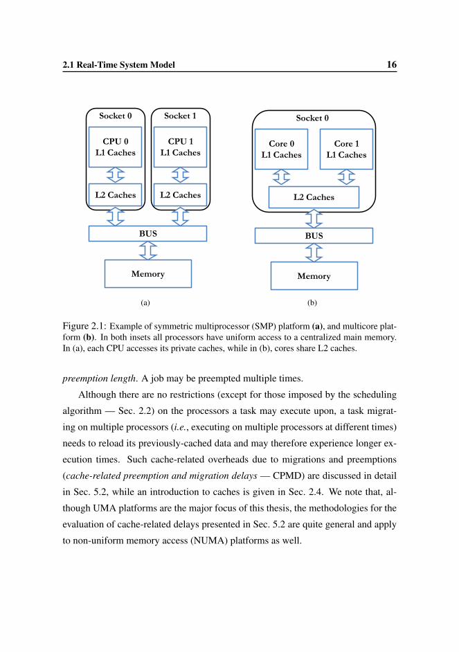
In this thesis, we consider the scheduling of real-time tasks on m (≥ 2) processors
P1, . . . , Pm. Specifically, we mainly focus on identical multiprocessor platforms,
where all processors have the same characteristics, such as speed and uniform access
time to memory (uniform memory access — UMA). In UMA platforms, all proces-
sors share a centralized memory that can be accessed by processors through a shared
interconnection bus. To alleviate high memory latencies, modern processors employ
a hierarchy of fast cache memories that contain recently-accessed instructions and
operands. These caches (more details on caches will be provided in Sec. 2.4) can be
exclusively accessed by single processors (as in symmetric multiprocessor –SMP–
platforms; Fig. 2.1(a)), or may be shared among two or more cores (i.e., processing
units placed within the same socket that share some resources such as caches, inter-
connection buses, etc.). Fig. 2.1(b) shows an example of a multicore platform with
shared caches.1
Tasks are equally capable to run on any processor, but the parallel execution
of the same task on multiple processors is not allowed. We say that a job T ji is
preempted if its execution is temporarily paused before it is completed, e.g., in favor
of another job with higher priority. Suppose Ti is preempted at time tp on processor
P and resumes execution at time tr on processor R. T ji is said to have incurred a
preemption if P = R, and a migration otherwise. In either case, we call tr − tp the
1In most of the thesis, we use the terms processor and core interchangeably; we explicitly disam-biguate the terms when such a distinction is important.
2.1 Real-Time System Model 16
CPU 0
L1 Caches
CPU 1
L1 Caches
L2 Caches L2 Caches
BUS
Memory
Socket 0 Socket 1
Core 0
L1 Caches
Core 1
L1 Caches
L2 Caches
BUS
Memory
Socket 0
(a)
CPU 0
L1 Caches
CPU 1
L1 Caches
L2 Caches L2 Caches
BUS
Memory
Socket 0 Socket 1
Core 0
L1 Caches
Core 1
L1 Caches
L2 Caches
BUS
Memory
Socket 0
(b)
Figure 2.1: Example of symmetric multiprocessor (SMP) platform (a), and multicore plat-form (b). In both insets all processors have uniform access to a centralized main memory.In (a), each CPU accesses its private caches, while in (b), cores share L2 caches.
preemption length. A job may be preempted multiple times.
Although there are no restrictions (except for those imposed by the scheduling
algorithm — Sec. 2.2) on the processors a task may execute upon, a task migrat-
ing on multiple processors (i.e., executing on multiple processors at different times)
needs to reload its previously-cached data and may therefore experience longer ex-
ecution times. Such cache-related overheads due to migrations and preemptions
(cache-related preemption and migration delays — CPMD) are discussed in detail
in Sec. 5.2, while an introduction to caches is given in Sec. 2.4. We note that, al-
though UMA platforms are the major focus of this thesis, the methodologies for the
evaluation of cache-related delays presented in Sec. 5.2 are quite general and apply
to non-uniform memory access (NUMA) platforms as well.
2.2 Real-Time Scheduling 17
2.2 Real-Time Scheduling
Scheduling algorithms are the third component of the real-time system model in-
troduced in Sec. 2.1. A scheduling algorithm defines the allocation of tasks to re-
sources at all time, defining therefore which jobs should run next on the available
processors. Ensuring that all jobs complete before their deadlines clearly depends
on the employed scheduling algorithm. In a system, the scheduler is the module that
implements a scheduling algorithm. A schedule is the assignment (produced by a
scheduler) of all the jobs in the system on the available processors. We assume that
the scheduler only produces valid schedules, i.e., schedules that are in agreement
with the task and resource models described above. Particularly, in a valid sched-
ule: (i) every processor is assigned to at most one job at any time, (ii) every job is
scheduled on at most one processor at any time, (iii) jobs are not scheduled before
their release time, and (iv) precedence constraints among jobs are satisfied.
A task set τ is feasible on a given hardware platform if there exists a sched-
ule (feasible schedule) in which every job of τ complete by its deadline. A HRT
system τ is said to be (HRT) schedulable on a hardware platform by algorithm Aif A always produces a feasible schedule for τ (i.e., no job of τ misses its dead-
line under A). A is an optimal scheduling algorithm if A correctly schedules every
feasible task system. When SRT systems are considered, a SRT system τ is (SRT)
schedulable under the scheduling algorithmA if the maximum deadline tardiness is
bounded.
The schedulable utilization bound (or utilization bound) is a metric commonly
used to compare different scheduling algorithms with respect to their effectiveness
in correctly scheduling task systems on hardware platforms. If Ub(A) is a utilization
bound for the scheduling algorithm A, then A can correctly schedule every task
system τ with U(τ) ≤ Ub(A). We note that, unless an optimal utilization bound is
known for A (e.g., in the EDF case below), using the schedulable utilization bound
to evaluate whether all jobs in a task set τ will meet their deadlines under A is a

2.2 Real-Time Scheduling 18
sufficient, but not necessary, schedulability test. In fact, there may exist a task set τ
with U(τ) > Ub(A) that is schedulable using A.
Given a set Γ of feasible task sets, the performance of a scheduling algorithm
A can be characterized as the fraction of task sets in Γ that are schedulable (HRT
or SRT) using A. This fraction is the schedulability of A and can be measured by
applying an appropriate schedulability test to each task set in Γ. Schedulability is
an interesting metric because it estimates the probability (for Γ with a sufficiently
large cardinality) that a set of tasks similar (with respect to their parameters) to
those in Γ is schedulable. “Good” scheduling algorithms should therefore have
high schedulability (ideally, 1.0, i.e., each tested task set in Γ is schedulable).
2.2.1 Uniprocessor Scheduling
Several approaches have been developed to schedule task systems on single-processor
platforms. In this section we only focus on two prominent scheduling algorithms
(RM and EDF) that have been the subject of intense research in the uniprocessor
scheduling field. Under the well known rate-monotonic (RM) scheduling algorithm,
tasks are statically prioritized according to their periods (tasks with smaller periods
have higher priority), while under earliest-deadline-first (EDF) scheduling algo-
rithm, jobs with earlier deadlines have higher priority (task priorities are dynami-
cally determined by the priorities of currently-released jobs).
In [83], Liu and Layland showed that RM is optimal among fixed-priority al-
gorithms and they derived a schedulable utilization bound for RM for periodic task
systems (this bound was later improved by Bini et al., [31]). RM has been particu-
larly important in real implementations since its (utilization-bound-based) schedu-
lability tests have polynomial complexity, and RM can be easily implemented on
top of FIFO scheduling policy, which is available in virtually all operating systems.
The EDF scheduling algorithm can schedule every feasible task system on a
single-processor platform (i.e., EDF is optimal on uniprocessor systems). In fact,
an implicit-deadline task system τ is schedulable under EDF on a uniprocessor plat-
2.2 Real-Time Scheduling 19
T1
T2
T3
0 5 10 15 20 25
T 11 T 2
1 T 31 T 4
1 T 51 T 6
1 T 71 T 8
1 T 91
T 12 T 2
2 T 32 T 4
2
T 13 T 2
3 T 33
T 52
(a)
T1
T2
T3
0 5 10 15 20 25
T 11 T 2
1 T 31 T 4
1 T 51 T 6
1 T 71 T 8
1 T 91
T 12 T 2
2 T 32 T 4
2 T 52
T 13 T 2
3 T 33T 1
3
T 22
T 33
T 52
(b)
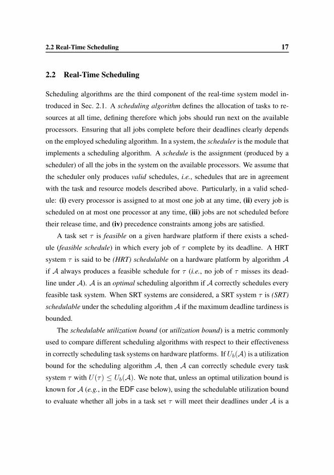
Figure 2.2: Example of uniprocessor schedules under (a) EDF, and (b) RM for a tasksystem with three tasks T1 = (1, 3), T2 = (2, 5), and T3 = (2, 8). Note that T3 missesits deadline at time 8 under RM. In this and in the following schedule examples, up-arrowsdenote job releases, and down-arrows indicate job deadlines. Deadline misses are indicatedby lightning bolt-shaped arrows.
form if U(τ) ≤ 1 = Ub(EDF) [83]. Despite its optimality, EDF scheduling policy
is employed in few real-world operating systems [56, 57, 58, 119], mainly because
mapping task priorities to task deadlines is thought to be somewhat complicated.
Partial schedules under RM and EDF are shown in Fig. 2.2 for the first few jobs
of a task system with three tasks T1 = (1, 3), T2 = (2, 5), and T3 = (2, 8).
2.2.2 Multiprocessor Scheduling
Extending uniprocessor scheduling algorithms to multiprocessor platforms is not as
straightforward as it may seem. Perhaps surprisingly, in the real-time computing

2.2 Real-Time Scheduling 20
Core 0 Core 1L2
L3
Core 2 Core 3L2
Socket 0
Figure 2.3: Partitioned scheduling on a quad-core platform with a two-level cache hier-archy. Tasks are statically assigned to cores and cannot migrate (this is indicated by thecircular arrow — compare to Fig. 2.4 and 2.5).
field an increase in the number of available processors does not always cause an
improvement in the performance of a task set. As described by Graham in 1976 [62],
adding resources (e.g., an extra processor) or relaxing constraints (e.g., removing
task precedence constraints or reducing execution time requirements) of a task set
that is optimally scheduled on a multiprocessor platform can increase the length of
the schedule.
Two basic approaches exist for scheduling real-time tasks on multiprocessor
platforms. In the partitioned approach, each task is statically assigned to a single
processor and migration is not allowed; in the global approach, tasks can freely
migrate and execute on any processor. Unfortunately, both approaches suffer draw-
backs that limit the achievable processor utilization.
Partitioned scheduling algorithms (Fig. 2.3) have the advantage that uniproces-
sor scheduling algorithms can be separately used on each processor, and such poli-
cies generally entail low preemption/migration costs. The disadvantage of parti-
tioned algorithms is that they require a bin-packing-like problem to be solved to as-
2.2 Real-Time Scheduling 21
L2
L3
L2
Socket 0
Core 0 Core 1
Core 2 Core 3
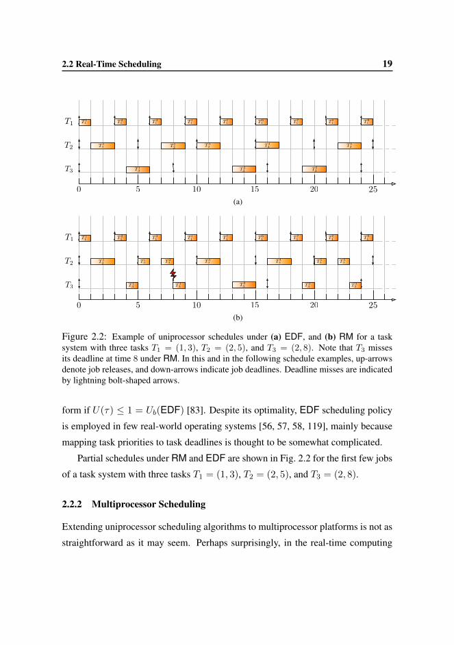
Figure 2.4: Global scheduling on a quad-core platform with a two-level cache hierarchy.Tasks can freely migrate on all the cores.
sign tasks to processors. Because of such bin-packing connections,2 the assignment
of tasks to processors is usually performed using heuristics (e.g., first-fit, best-fit,
next-fit, worst-fit), but restrictive caps on total utilization are generally required to
ensure timing constraints for both HRT and SRT systems.
Under global approaches, tasks are selected from a single run queue and may
migrate among processors (Fig. 2.4). Contrary to partitioning, restrictive caps on
total utilization can be avoided under global approaches for both HRT [7] and
SRT [80] systems. In HRT systems, if tasks can freely migrate among processors,
Pfair algorithms [7, 21, 81, 109] such as PD2 can optimally schedule a task sys-
tem τ if U(τ) ≤ m.3 In SRT systems, a wide variety of (dynamic-priority) global
real-time scheduling algorithms ensure bounded tardiness for implicit-deadline task
systems [79, 80] (i.e., such systems can be optimally scheduled on multiprocessors
by dynamic-priority global scheduling algorithms). However, due to contention for
the global run queue and non-negligible migration overheads among processors,2The bin-packing problem is NP-hard in the strong sense [59].3Some Pfair algorithms may pose some restrictions on deadlines, periods, and execution times
(e.g., PD2 [7] requires implicit-deadline task systems, with integral periods and execution times).
2.2 Real-Time Scheduling 22
L2
L3
L2
Socket 0
Core 0 Core 1
Core 2 Core 3
L2 Cluster
L2 Cluster
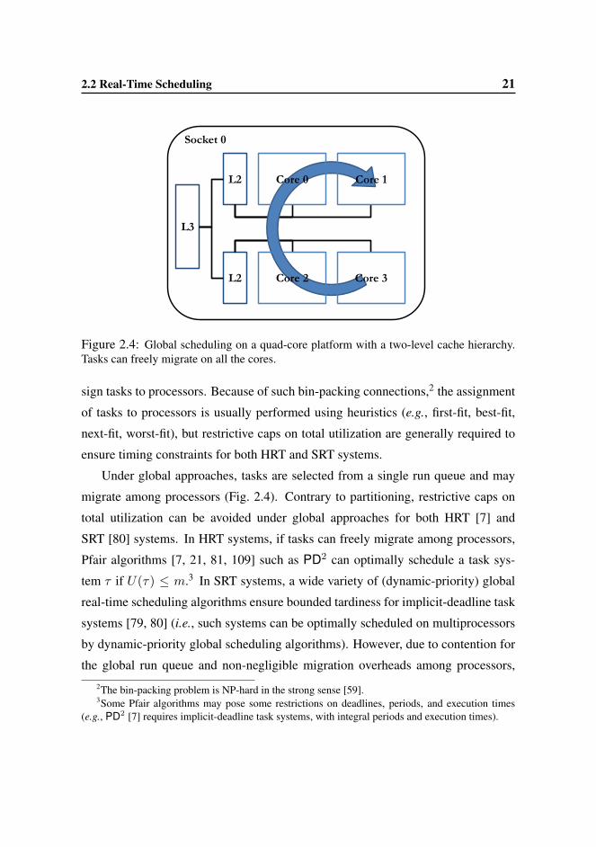
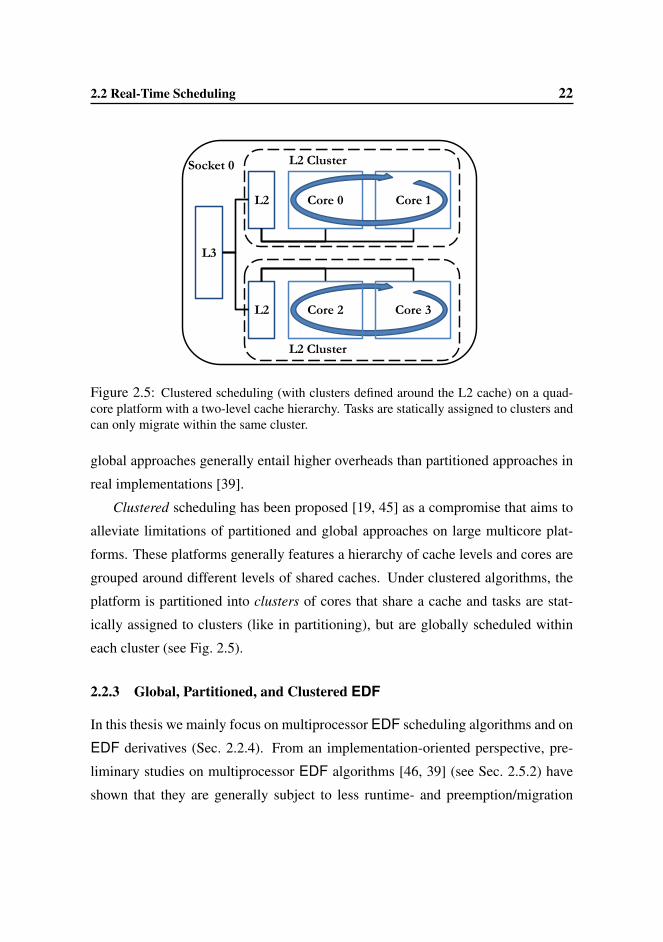
Figure 2.5: Clustered scheduling (with clusters defined around the L2 cache) on a quad-core platform with a two-level cache hierarchy. Tasks are statically assigned to clusters andcan only migrate within the same cluster.
global approaches generally entail higher overheads than partitioned approaches in
real implementations [39].
Clustered scheduling has been proposed [19, 45] as a compromise that aims to
alleviate limitations of partitioned and global approaches on large multicore plat-
forms. These platforms generally features a hierarchy of cache levels and cores are
grouped around different levels of shared caches. Under clustered algorithms, the
platform is partitioned into clusters of cores that share a cache and tasks are stat-
ically assigned to clusters (like in partitioning), but are globally scheduled within
each cluster (see Fig. 2.5).
2.2.3 Global, Partitioned, and Clustered EDF
In this thesis we mainly focus on multiprocessor EDF scheduling algorithms and on
EDF derivatives (Sec. 2.2.4). From an implementation-oriented perspective, pre-
liminary studies on multiprocessor EDF algorithms [46, 39] (see Sec. 2.5.2) have
shown that they are generally subject to less runtime- and preemption/migration

2.2 Real-Time Scheduling 23
overheads than Pfair algorithms. Furthermore, from the standpoint of schedulability,
dynamic-priority multiprocessor algorithms are generally superior to fixed-priority
algorithms [47]. In fact, the set of task sets that are schedulable by the class of mul-
tiprocessor fixed-priority algorithms is a proper subset of the set of task sets that are
schedulable by the class of multiprocessor dynamic-priority algorithms (as long as
such a comparison is performed with respect to the same migration class) [47]. In
addition, global multiprocessor EDF algorithms are optimal for SRT systems [54].
Under partitioned EDF (P-EDF), once tasks have been assigned to proces-
sors, EDF scheduling algorithm is employed as uniprocessor scheduling algorithm.
Given the bin-packing connections noted above, not all task sets can be success-
fully partitioned under P-EDF and caps on total utilization are required to ensure
timing constraints. Particularly, to schedule an implicit-deadline task system τ up
to (2 ·U(τ)−1) processors may be required [86]. This means that, to ensure timing
constraints, up to half of the available processors may be unused by P-EDF in the
long run.
Similarly to P-EDF, in a HRT system, the global EDF (G-EDF) scheduling
algorithm also requires up to (2 · U(τ) − 1) processors to feasibly schedule a task
system τ where the maximum per-task utilization is max(ui) ≤ 1/2 [22]. (More
processors may be required if max(ui) > 1/2 [61].) In 1978, Dhall and Liu noted
that on multiprocessor platforms (m ≥ 2) there exist task sets with total utiliza-
tion close to 1.0 that cannot be scheduled (HRT) by G-EDF or global RM [55].
Mainly because of this observation (the so-called “Dhall effect”), in early research
on multiprocessor scheduling algorithms, global approaches did not receive much
attention, and most results concerning G-EDF and global scheduling algorithms are
quite recent. As already noted above, when SRT systems are considered, G-EDF
ensures bounded deadline tardiness as long as the system is not overutilized [54].
Partial schedules for the first few jobs under P-EDF, and G-EDF for a task
system with four tasks T1 = (2, 3), T2 = (3, 8), T3 = (1, 7), and T4 = (5, 7) are
shown in Fig. 2.6.

2.2 Real-Time Scheduling 24
T1
T2
T3
T4
P1 P2
0 5 10 15 20 25
T 24 T 3
4T 14
T 11 T 2
1 T 31 T 4
1 T 51 T 6
1 T 71
T 12 T 3
2
T 13 T 2
3 T 33
T 22
(a)
T1
T2
T3
T4
P1 P2
0 5 10 15 20 25
T 24 T 3
4T 14
T 11 T 2
1 T 31 T 4
1 T 51 T 6
1 T 71
T 12 T 3
2
T 13 T 2
3 T 33
T 22T 2
2
(b)
Figure 2.6: Example of multiprocessor schedules under (a) P-EDF, and (b) G-EDF for atask system τ with four tasks T1 = (2, 3), T2 = (3, 8), T3 = (1, 7), and T4 = (5, 7). Notethat for any partitioning of τ onto two processors, the total utilization of the tasks assignedto one processor is greater than one. Therefore τ cannot be scheduled under P-EDF on twoprocessors in such a way that all tasks meet their deadlines. In fact, in inset (a), T1 missesits deadline at time 9 and 18, and T2 misses its deadline at time 16. Note that under G-EDF(b), T 2
2 migrates from processor P1 to processor P2.

2.2 Real-Time Scheduling 25
Clustered EDF (C-EDF) was proposed [19, 45] as a compromise between P-
EDF and G-EDF for large multicore platforms where a hierarchy of cache mem-
ories is employed. On such platforms, caches are organized in levels where the
fastest (and usually smallest) caches are denoted as level-1 (L1) caches, with deeper
caches (L2, L3, etc.) being successively larger and slower. Generally, L1 caches are
private per-core caches, while L2 and L3 caches are shared among a progressively
larger number of cores. In C-EDF, all cores that share a specific cache level (L2 or
L3) are defined to be a cluster; tasks are allowed to migrate within a cluster, but not
across clusters. Clustering lowers migration costs and lessens run-queue contention
in comparison to G-EDF, and eases bin-packing problems associated with P-EDF.
In particular, bin packing becomes easier because clustering results in fewer, larger
bins. Under C-EDF, deadline tardiness is bounded if the total utilization of the
tasks assigned to each cluster is at most the number of cores per cluster. We use the
notation C-EDF-L2 (C-EDF-L3) when we wish to specifically indicate that each
cluster is defined to include all cores that share an L2 (L3) cache.
We note that P-EDF and G-EDF can be seen as special cases of C-EDF: in
P-EDF, each cluster consists of only one core, while in G-EDF, all cores form one
cluster.
2.2.4 Semi-Partitioned Multiprocessor Algorithms
Semi-partitioned multiprocessors scheduling algorithms are another compromise
between pure partitioning and global scheduling. Semi-partitioning extends par-
titioned scheduling by allowing a small number of tasks to migrate, improving
schedulability. Such tasks are called migratory, in contrast to fixed tasks that do
not migrate. Semi-partitioned scheduling was originally proposed by Anderson et
al. [5] for SRT systems. Subsequently, other authors developed semi-partitioned al-
gorithms for HRT systems [8, 9, 33, 72, 75]. The common goal in all of this work is
to circumvent the algorithmic limitations and resulting capacity loss of partitioning
while avoiding the overhead of global scheduling by limiting migrations.

2.3 Operating System and Hardware Capabilities 26
Among the semi-partitioned scheduling algorithms that have been proposed,
this thesis focuses on three algorithms, each of which uses earliest-deadline-first
(EDF) prioritizations in some way: EDF-fm, EDF-WM, and NPS-F (and its “clus-
tered” variant C-NPS-F). These algorithms are described in detail in Ch. 4. EDF-
fm, EDF-WM, and NPS-F are subject to less schedulability-related capacity loss
than static-priority semi-partitioned algorithms and other related dynamic-priority
semi-partitioned algorithms (many of which were precursors to these algorithms).
Related work and an overview of other semi-partitioned algorithms are discussed in
Sec. 2.5.3.
In the semi-partitioned algorithms considered in this thesis, a task Ti may be
assigned fractions (shares) of its utilization on multiple processors. We denote with
si,j the share that a task Ti requires on processor Pj . If Ti has non-zero shares on
the processors in the set Π, then we require∑
Pj∈Π si,j = ui. Letting τj be the set
of tasks assigned to processor Pj , the assigned capacity on Pj is cj =∑
Ti∈τj si,j .
The available capacity on Pj is thus 1 − cj . We denote with T xi,j the x-th job of a
task Ti that is assigned to Pj .
2.3 Operating System and Hardware Capabilities
This section offers an introduction of common services provided by OSs and by
hardware platforms. Such services play an important role in understanding the de-
sign of the algorithms investigated in this thesis.
The algorithms evaluated in this dissertation were implemented and evaluated
within LITMUSRT [119], which is a real-time extension of the Linux kernel that
allows schedulers to be developed as plugin components. LITMUSRT will be de-
scribed in details in Ch. 3.

2.3 Operating System and Hardware Capabilities 27
2.3.1 Run Queues
Many modern operating systems (including Linux) provide a scheduling framework
that employs per-processor run queues. Accesses to the state of a task are syn-
chronized by acquiring the lock of the run queue that currently contains that task.
Therefore, holding a run-queue lock gives the owner the right to modify not only
the run-queue state, but also the state of all tasks in the run queue.
Migrating a task under this locking rule requires local and remote run-queue
locks to be acquired. Under scheduling algorithms that allow concurrent migra-
tions, complex coordination is required to ensure that deadlocks do not occur. This
has drawbacks for the implementation of global scheduling algorithms that may mi-
grate tasks when making a scheduling decision (i.e., while holding the run-queue
lock). In Linux (and in LITMUSRT) to avoid deadlock during a migration, the
current run-queue lock has to be released,4 opening a dangerous windows of time
where the state of the migrating task may be modified. In such a context, when con-
current scheduling decisions happen, ensuring that migratory tasks will be executed
by a single processor only (i.e., only one processor may use a task’s process stack)
is quite challenging. Algorithms where the likelihood of simultaneous scheduling
decisions is high may thus entail rather high scheduling overheads.
2.3.2 Inter-Processor Interrupts (IPIs)
IPIs are the only way to programmatically notify a remote processor of a local event
(such as a job release) and are used to invoke the scheduler. Despite their small
latencies, IPIs are not “instantaneous” and task preemptions based on IPIs incur an
additional delay.4Consider a task migration from CPU A to CPU B. CPU A needs to acquire the run-queue lock of
CPU B before the migration can occur. If CPU B is performing the same operation (migrating a taskfrom CPU A) and neither CPU releases its local run-queue lock, then deadlock occurs.

2.4 Kernel Overheads and Caches 28
2.3.3 Timers and Time Resolution
Modern hardware platforms feature several clock devices and timers that can be
used to enforce real-time requirements. While such devices typically offer high
resolutions (≤ 1µs), hardware latencies and the OS’s timer management overheads
considerably decrease the timer resolutions available both within the kernel and at
the application level [66, 104]. Furthermore, in Linux (for the x86 architecture),
high-resolution timers are commonly implemented based on per-processor devices.
As some of the evaluated algorithms require timers to be programmed on remote
processors, LITMUSRT uses a two-step timer transfer operation: an IPI is sent to
the remote CPU where the timer should be armed; after receiving the IPI, the remote
CPU programs an appropriate local timer (see Sec. 2.4 and Fig. 2.7). Therefore, as
two operations are needed to set up remote timers, scheduling algorithms that make
frequent use of such timers incur higher overheads.
2.4 Kernel Overheads and Caches
In actual implementations of scheduling policies, tasks are delayed by seven major
sources of system overhead, five of which are illustrated in Fig 2.7.5 When a job
is released, release overhead is incurred, which is the time needed to service the
interrupt routine that is responsible for releasing jobs at the correct times. When-
ever a scheduling decision is made, scheduling overhead is incurred while select-
ing the next process to execute and re-queuing the previously-scheduled process.
Context-switch overhead is incurred while switching the execution stack and pro-
cessor registers. These overhead sources occur in sequence in Fig. 2.7, on processor
P1 at times 0 and 4.2 when T x1,1 and T z3 are released, and again on processor P2 at
times 0.5 and 7 when T y2 and T x+11,2 are released. IPI latency is a source of overhead
that occurs when a job is released on a processor that differs from the one that will5Fig 2.7 depicts a schedule for EDF-fm. This semi-partitioned algorithm is described in detail in
Sec. 4.1.

2.4 Kernel Overheads and Caches 29
P1
P2
0 5 10 15
csr
csr
csr
csr cst
rT1,1
T4
T3
T1,2T2
IPI latencytimer transfer
context switchrelease schedule
Figure 2.7: Example EDF-fm schedule with overheads for five jobs T x1,1 = T x+1
1,2 =(2.7, 7), T y
2 = (5, 10), T z3 = (6, 11), and Tw
4 = (3, 5) on two processors (P1, P2). T x1,1
and T x+11,2 belong to a migratory task T1 whose shares are assigned on P1 and P2. Large
up-arrows denote interrupts, small up-arrows denote job releases, down-arrows denote jobdeadlines, T-shaped arrows denote job completions, and wedged boxes denote overheads(which are magnified for clarity). Job releases occur at rx1,1 = 0, rx+1
1,2 = rx1,1 + p1 =7, ry2 = 0.5, rz3 = 4.2, and rw4 = 11.
schedule it. This situation is depicted in Fig. 2.7, where at time 11, Tw4 is released on
P1, which triggers a preemption on P2 by sending an IPI. Timer-transfer overhead
is the overhead incurred when programming a timer on a remote CPU (see Sec. 2.3).
In Fig. 2.7, this overhead is incurred on processor P2 at time 4.5 when the comple-
tion of the job T x1,1 (on processor P1) of the migratory task T1 triggers a request to
program a timer on processor P2 to enable the release of the next job T x+11,2 . We
note that timer-transfer overheads are only incurred under semi-partitioned schedul-
ing algorithms such as EDF-fm and EDF-WM (discussed in Ch. 4). Under multi-
processor EDF scheduling algorithms such as P-EDF, G-EDF, and C-EDF, tasks
program timers on the local CPU where they are residing and therefore, no timer-
transfer overheads are incurred. The same holds under the NPS-F semi-partitioned
algorithm, where each task always executes within its server. Tick overhead is the
time needed to manage periodic scheduler-tick timer interrupts; such interrupts have
limited impact under event-driven scheduling (such as EDF) and, for clarity, they
are not not shown in Fig. 2.7. Finally, cache-related preemption and migration de-
lay (CPMD) accounts for additional cache misses that a job incurs when resuming

2.4 Kernel Overheads and Caches 30
execution after a preemption or migration. The temporary increase in cache misses
is caused by the perturbation of caches while the job was not scheduled.
Contrary to the other kernel overheads, measuring CPMD is a difficult prob-
lem [39]: CPMD can only be observed indirectly and is heavily dependent on the
working set size (WSS) of each task. In Sec. 5.2 we present two methods to empiri-
cally measure CPMD, while in the following section we provide some background
on caches.
Caches. Modern processors employ a hierarchy of fast cache memories that con-
tain recently-accessed instructions and operands to alleviate high off-chip memory
latencies. Caches are organized in layers (or levels), where the fastest (and usu-
ally smallest) caches are denoted level-1 (L1) caches, with deeper caches (L2, L3,
etc.) being successively larger and slower. A cache contains either instructions or
data, and may contain both if it is unified. In multiprocessors, shared caches serve
multiple processors, in contrast to private caches, which serve only one.
Caches operate on blocks of consecutive addresses called cache lines with com-
mon sizes ranging from 8 to 128 bytes. In direct mapped caches, each cache line
may only reside in one specific location in the cache. In fully associative caches,
each cache line may reside at any location in the cache. In practice, most caches are
set associative, wherein each line may reside at a fixed number of locations.
The set of cache lines accessed by a job is called the working set (WS) of the
job; workloads are often characterized by their working set sizes (WSSs). A cache
line present in a cache is useful if it is going to be accessed again. If a job references
a cache line that cannot be found in a level-X cache, then it suffers a level-X cache
miss. This can occur for several reasons. Compulsory misses are triggered the
first time a cache line is referenced. Capacity misses result if the WSS of the job
exceeds the size of the cache. Further, in direct mapped and set associative caches,
conflict misses arise if useful cache lines were evicted to accommodate mapping
constraints of other cache lines. If a shared cache does not exceed the combined

2.5 Related Work 31
WS of all jobs accessing it, frequent capacity and conflict misses may arise due to
cache interference. Jobs that incur frequent level-X capacity and conflict misses
even if executing in isolation are said to be thrashing the level-X cache.
Cache affinity describes the effect that a job’s overall cache miss rate tends to
decrease with increasing execution time (unless it thrashes all cache levels)—after
an initial burst of compulsory misses, most useful cache lines have been brought
into a cache and do not cause further misses. This explains cache-related preemp-
tion delays: when a job resumes execution after a preemption, it is likely to suffer
additional capacity and conflict misses as the cache was perturbed [84]. Migrations
may further cause affinity for some levels to be lost completely (depending on cache
sharing), thus adding compulsory misses to the penalty.
A job’s memory references are cache-warm after cache affinity has been estab-
lished; conversely, cache-cold references imply a lack of cache affinity.
In this thesis, we restrict our focus to cache-consistent shared-memory ma-
chines: when updating a cache line that is present in multiple caches, inconsisten-
cies are avoided by a cache consistency protocol, which either invalidates outdated
copies or propagates the new value.
2.5 Related Work
In this section we summarize previous studies on the topics that are the subject of
this thesis. In particular, we provide related work regarding the estimation of cache-
related preemption and migration delays, related work concerning the evaluation of
multiprocessor scheduling policies under consideration of measured overheads, and
prior work on semi-partitioned algorithms.
2.5.1 Prior Work on Cache-Related Delays
Accurately assessing cache-related delays is a classical component of worst-case
execution time (WCET) analysis [121], in which an upper bound on the maximum
2.5 Related Work 32
resource requirements of a real-time task is derived a priori based on control- and
data-flow analysis. Unfortunately, predicting cache contents and hit rates is no-
toriously difficult: even though there has been some initial success in bounding
cache-related preemption delays (CPDs) caused by simple data [103] and instruc-
tion caches [113], analytically determining preemption costs on uniprocessors with
private caches is still generally considered to be an open problem [121]. Thus,
on multicore platforms with a complex hierarchy of shared caches, we must—
at least for now—resort to empirical approximation. However, given recent ad-
vances in bounding migration delays [65] and analyzing interference due to shared
caches [48, 123, 106], we expect multicore WCET analysis to be developed eventu-
ally.
Trace-driven memory simulation [118], in which memory reference traces col-
lected from actual program executions are interpreted with a cache simulator, has
been applied to count cache misses after context switches [93, 112]. Using traces
from throughput-oriented workloads, Mogul and Borg [93] estimated CPDs to lie
within 10µs to 400µs on an early ’90s RISC-like uniprocessor with caches ranging
in size from 64 to 2048 kilobytes. In work on real-time systems, Starner and As-
plund [112] used trace-driven memory simulation to study CPDs in benchmark tasks
on a MIPS-like uniprocessor with small caches. As the simulation environment is
fully controlled, this method allows cache effects to be studied in great detail, but it
is also limited by its reliance on accurate architectural models (which may not al-
ways be available) and representative memory traces (which are difficult to collect
due to complex instrumentation requirements).
Several probabilistic models have been proposed to predict expected cache misses
on uniprocessors [3, 84, 115]. In the context of evaluating (hard) real-time sched-
ulers, such models apply only to a limited extent because it is difficult to extract
bounds on the worst-case number of cache misses. Further, they rely on task pa-
rameters that are difficult to obtain or predict (e.g., cache access profiles [84]), and
do not predict cache misses after migrations.
2.5 Related Work 33
Closely related to the approach adopted in this thesis are several recent CPD mi-
crobenchmarks [51, 82, 117]. Li et al. [82] measured the cost of switching between
two processes that alternate between accessing a data array and communicating via
a pipe on an Intel Xeon processor with a 512 KB L2 cache, and found that average
case CPDs can range from around 100µs to 1500µs, depending on array size and
access pattern. In the context of real-time systems, Li et al.’s experimental setup is
limited because it can only estimate average-case, but not worst-case, delays. David
et al. [51] measured preemption delays in Linux kernel threads on an embedded
ARM processor with comparably small caches and observed CPDs in the range of
60µs to 120µs. Tsafrir [117] investigated the special case in which the scheduled
job is not preempted, but cache contents are perturbed by periodic clock interrupts,
and found that slowdowns vary heavily among workloads. None of the cited empir-
ical studies considered job migrations.
Once bounds on cache-related delays are known for a given task set, they must
be accounted for during schedulability analysis. This is typically accomplished
by inflating task parameters to reflect the time lost to reloading cache contents.
Straightforward methods are known for common uniprocessor schedulers [27, 42,
69] and have also been derived for global schedulers [53, 109]; we use this approach
in Sec 6.3. Other methods that yield tighter bounds by analyzing per-task cache use
and the instant at which each preemption occurs have been developed for static-
priority uniprocessor schedulers [78, 98, 113]. However, similar to WCET analysis,
these methods have not yet been generalized to multiprocessors since they require
useful cache contents to be predicted accurately. Stamatescu et al. [110] propose
including average memory access costs in specific analysis, but do not report mea-
sured costs.
Several research directions orthogonal to this thesis are concerned with avoid-
ing, or at least reducing, cache-related delays in multiprocessor real-time systems.
On an architectural level, Sarkar et al. [105] have proposed a scheduler-controlled
cache management scheme that enables cache contents to be transferred in bulk in-

2.5 Related Work 34
stead of relying on normal cache-consistency updates. This can be employed to
lessen migration costs by transferring useful cache contents before a migrated job
resumes [105]. Likewise, Suhendra and Mitra [114] have considered cache locking
and partitioning policies to isolate real-time tasks from timing interference due to
shared caches. While promising, neither technique is supported in current multicore
architectures.
In work on real-time scheduling, cache-aware schedulers [44, 63], which make
shared caches an explicitly-managed resource, have been proposed to both prevent
interference in HRT systems [63] and to encourage data reuse in SRT systems [44].
2.5.2 Evaluation of Multiprocessor EDF Scheduling Algorithms
Most prior studies concerning the viability of supporting sporadic real-time work-
loads on symmetric multi-processor (SMP) and multicore platforms under consider-
ation of real-world overheads have been conducted at The University of North Car-
olina at Chapel Hill (UNC), (NC, USA). To facilitate this line of research, the UNC’s
“Real-Time Group” has developed LITMUSRT (LInux Testbed for MUltiprocessor
Scheduling in Real-Time systems— see Sec. 3.3 and [119]), a real-time Linux ex-
tension that was used in the related work presented in this section, and that was em-
ployed to obtain the results presented in this thesis (chapters. 5 and 6). To the best
of our knowledge, LITMUSRT is the only (published) real-time OS where global,
clustered and semi-partitioned real-time schedulers are supported.
In [46], Calandrino et al. evaluated five well-known multiprocessor real-time
scheduling algorithms on a four-processor (non-multicore) 32-bit 2.7 GHz Intel
Xeon SMP platform. On this small SMP platform, with relatively large private L2
caches, each tested algorithm proved to be the preferred choice in some of the tested
scenarios. In particular, global algorithms outperformed partitioned algorithms in
supporting SRT workloads.
In [39], Brandenburg et al. analyzed the scalability of several global, parti-
tioned, and clustered algorithms (including the EDF variants presented in Sec. 2.2).

2.5 Related Work 35
This evaluation was conducted on a much larger and slower multicore platform: a
SUN Niagara with a small single shared L2 cache and 32 logical processors, each
with an effective speed of 300 MHz. As before, each tested algorithm was found
to perform better than the others for some subset of the considered scenarios. Par-
ticularly, it was observed that global algorithms are heavily affected by run-queue-
related overheads. C-EDF exhibited schedulability in the HRT case that is interme-
diate between G-EDF and P-EDF. In the SRT case, C-EDF generally exhibited the
best schedulability, as well as lower tardiness than G-EDF.
In [37], Brandenburg and Anderson evaluated seven possible implementations
of G-EDF in LITMUSRT on the above-mentioned Niagara platform. Tradeoffs
involving implementation approaches were found to significantly impact schedula-
bility.
The idea of a clustered approach to ameliorate limitations of partitioned and
global approaches on large multiprocessor platforms was introduced by Calandrino et
al. [45] and Baker and Baruah [19]. Notably, Calandrino et al. presented guidelines
for defining clusters for SRT workloads. Empirical results were obtained by them
using the SESC architecture simulator for a 64-core platform.
Shin et al. [107] presented a study concerning virtual clusters. Virtual clusters
can share processors of the underlying platform, while physical clusters are com-
pletely independent. In this thesis, we focus on physical clusters only.
2.5.3 Evaluation of Semi-Partitioned Algorithms
This dissertation considers three semi-partitioned algorithms: EDF-fm, EDF-WM,
and NPS-F. EDF-fm is the original SRT semi-partitioned algorithm proposed by
Anderson et al. [5]. EDF-WM and NPS-F are HRT algorithms proposed by Kato et
al. [72] and Bletsas and Andersson [33], respectively. We further consider a “clus-
tered” variant of NPS-F that was proposed [33] to eliminate entirely off-chip migra-
tions in multi-socket systems (all cores on one chip are considered to be a “cluster”).
These algorithms are described in detail in Ch. 4.

2.5 Related Work 36
Other EDF-based semi-partitioned algorithms have also been proposed. These
include algorithms that were precursors to NPS-F [32, 8, 9, 12] and to EDF-
WM [72, 71].
To the best of our knowledge, detailed runtime overheads affecting semi-partitioned
algorithms have never been measured before within a real operating system, and the
schedulability of these algorithms under consideration of overheads has never been
evaluated. Nonetheless, some simulation-based studies (without consideration of
overheads) have been done. In [75], an algorithm called EDF-SS [9] (which is
a precursor of NPS-F) is compared to EDF-WM. In that study, EDF-SS exhib-
ited less schedulability-related capacity loss than EDF-WM in the majority of the
tested cases, at the cost of many more context switches (five to twenty times more,
in heavily utilized systems). For this reason, we believe that EDF-WM is a bet-
ter candidate than EDF-SS for an implementation-oriented study. Additionally, a
variant of EDF-WM called EDF-WMR that supports reservations has been imple-
mented within a framework called AIRS [70]. A proof-of-concept implementation
of an algorithm called EKG-sporadic [8], which is precursor of NPS-F, also has
been proposed in a technical report [13] and guidelines for implementing semi-
partitioned approaches in ADA have been recently given in [11]. DP-WRAP [81]
shares commonalities with EKG [12] (a precursor of NPS-F), but its design is not
implementation-oriented.
Although the focus of this dissertation is on EDF-based algorithms, fixed-priority
semi-partitioned scheduling has also been an active research topic [64, 73, 74, 77].
From a schedulability perspective they are generally inferior to EDF-based algo-
rithms and their evaluation is therefore deferred to future work.

Chapter 3
Real-Time Operating Systems
This chapter provides an overview of the most important predictability-related is-
sues tackled by real-time operating systems (RTOSs) and describes the major char-
acteristics of LITMUSRT, the real-time Linux variant employed in the evaluations
presented in this thesis.
The main focus of this chapter (and of this thesis in general) are Linux-based
real-time operating systems. In fact, given the availability of the source code and
the support of a wide range of architectures and devices, Linux has become a natu-
ral starting point to experiment and evaluate real-time features within a real-world
operating system (e.g., [89, 124, 30, 91, 57, 119]). In addition, real-time character-
istics of Linux have been recently enhanced with the incorporation of features such
as high-resolution timers, shortened non-preemptable sections, and priority inheri-
tance.
3.1 OS Latency and Jitter
As noted in Sec. 1.1, the objectives of an RTOS are to effectively support real-time
applications, by ensuring that application requirements will be met. Furthermore,
an RTOS should provide the infrastructure (interrupt handling routines, time man-
agement functions, etc.) to allow real-time applications to interact with the envi-
37
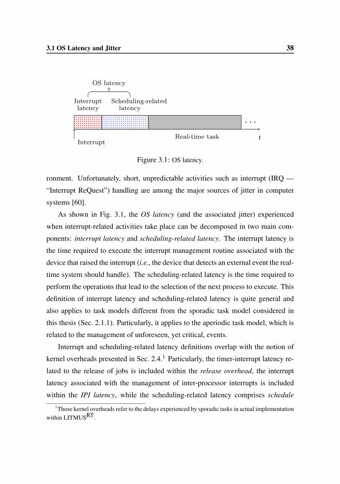
3.1 OS Latency and Jitter 38
tInterrupt
Interruptlatency
Scheduling-relatedlatency
OS latency
Real-time task
Real-time task
· · ·
1
Figure 3.1: OS latency.
ronment. Unfortunately, short, unpredictable activities such as interrupt (IRQ —
“Interrupt ReQuest”) handling are among the major sources of jitter in computer
systems [60].
As shown in Fig. 3.1, the OS latency (and the associated jitter) experienced
when interrupt-related activities take place can be decomposed in two main com-
ponents: interrupt latency and scheduling-related latency. The interrupt latency is
the time required to execute the interrupt management routine associated with the
device that raised the interrupt (i.e., the device that detects an external event the real-
time system should handle). The scheduling-related latency is the time required to
perform the operations that lead to the selection of the next process to execute. This
definition of interrupt latency and scheduling-related latency is quite general and
also applies to task models different from the sporadic task model considered in
this thesis (Sec. 2.1.1). Particularly, it applies to the aperiodic task model, which is
related to the management of unforeseen, yet critical, events.
Interrupt and scheduling-related latency definitions overlap with the notion of
kernel overheads presented in Sec. 2.4.1 Particularly, the timer-interrupt latency re-
lated to the release of jobs is included within the release overhead, the interrupt
latency associated with the management of inter-processor interrupts is included
within the IPI latency, while the scheduling-related latency comprises schedule1Those kernel overheads refer to the delays experienced by sporadic tasks in actual implementation
within LITMUSRT.

3.2 Problems of Predictability in Linux 39
overhead and context-switch overhead (see Sec. 2.4 and Fig. 2.7).
Jitter related to the OS latency (but also to the non-deterministic behavior of
commercial off-the-shelf — COTS — hardware platforms where many RTOSs ex-
ecute) conflicts with predictability, which is the most important feature that RTOSs
should provide. Most of the attention in the design of RTOSs is therefore directed
at increasing the predictability of critical OS execution paths (such as IRQ man-
agement routines) in such a way that the impact of OS latency jitter is bounded or
limited. This problem is particularly difficult on multiprocessor and multicore plat-
forms, because the activities performed by the OS are much more complicated and
because bounding the effects of shared caches is difficult (see Sec. 2.5.1).
3.2 Problems of Predictability in Linux
Considering its root as a general purpose operating system (GPOS), Linux is not
specifically designed for HRT. Particularly, the main issues of predictability under
Linux are related to:
• Non-preemptable critical sections. Several components of the kernel cannot
be preempted and interrupts are disabled during the execution of several IRQ
management routines. These factors lead to priority inversions and cause
unpredictability in the execution of critical real-time paths.
• Non-predictable duration of IRQ management routines. Even though Linux
employs a split-interrupt management schema,2 the duration of IRQ manage-
ment routines is non predictable (partially because of the non-preemptable
critical section issues mentioned above, and partially because IRQ manage-
ment routines can be nested in a last-in-first-out order), thus affecting the
predictability of the system.2Split-interrupt management provides a fast-acknowledgment to the hardware device that raised
the interrupt, while it may defer slower software interrupt management routines.

3.2 Problems of Predictability in Linux 40
• Throughput-oriented scheduling. The design of Linux is throughput oriented
and scheduling decisions on multiprocessor systems evenly distribute the work-
load on all available CPUs, regardless of process priorities. This may cause
unneeded migrations and additional overheads that impact the predictability
of the system.3
Despite these limitations, it has been claimed that Linux can handle a large and
important subset of real-time applications. As noted by McKenney [92] in 2005,
I believe that Linux is ready to handle applications requiring sub-
millisecond process-scheduling and interrupt latencies with 99.99+ per-
cent probabilities of success. No, that does not cover every imaginable
real-time application, but it does cover a very large and important sub-
set.
Despite this claim, there exist applications where the above-mentioned predictabil-
ity issues are critical, and that require microsecond process-scheduling and interrupt
latencies. In order to support these applications, mono- and dual-kernel approaches
have been proposed.4
Mono-kernel approach. Under this approach, higher predictability is achieved
by addressing the culprits noted above through modifications of the Linux ker-
nel. This approach is followed by some commercial RTOSs (e.g., MontaVista
Linux [96], timesys [116], etc.) and by the open-source CONFIG PREEMPT -
RT Patch of the Linux kernel [91, 95]. Particularly, the CONFIG PREEMPT RT
Patch enables the “full preemption” of the kernel, by de-facto removing all non-
preemptable critical sections, thus bounding priority inversions. Furthermore, un-
der the CONFIG PREEMPT RT Patch, IRQ management routines run in process3The impacts of this predictability issue can be limited through the use of partitioned multiproces-
sor scheduling policies.4Even though mono- and dual-kernel approaches particularly target Linux-based systems, dual-
kernel and micro-kernel concepts also apply to other non-Linux-based RTOSs (e.g., VxWorks [122]).

3.2 Problems of Predictability in Linux 41
RTOS
High Prio
HAL
Hardware
RT Apps.
RTOS
Low Prio
RT Apps.
GPOS
Apps.
Figure 3.2: Example of dual-kernel approach. The HAL layer virtualizes the hardwarefor the three OSs that concurrently execute on top of the HAL. Interrupts are dispatchedaccording to OS priorities: the high priority RTOS is the first to manage them, followed bythe low priority RTOS, and finally by the GPOS.
context (IRQ threading), thus limiting the unpredictability related to their execu-
tion (IRQ routines are assigned a priority and are scheduled like normal real-time
tasks). In addition, under the CONFIG PREEMPT RT Patch, the fixed-priority real-
time scheduling policy employed by Linux is modified to take into account process
priorities during load-balancing operations on multiprocessor platforms.
Dual-kernel approach. Under this approach, a virtualization layer is employed
to concurrently execute two (or more) operating systems (which can be considered
virtual machines with different priorities) on the same hardware. The virtualization
layer (hardware abstraction layer — HAL) delivers interrupts (raised by hardware
devices) according to the priority of the concurrent OSes, and ensures isolation
among OSs (see Fig. 3.2). Although the abstraction layer may introduce addi-
tional latencies, the dual-kernel approach allows to isolate GPOSs like Linux from
RTOSs, thus avoiding the predictability issues mentioned above. Therefore, under
dual-kernel approaches, actual real-time guarantees are not based on Linux itself,
but on the abstraction layer and on the real-time capabilities of the RTOS execut-

3.3 LITMUSRT 42
ing on top of the HAL.5 Linux-derived RTOSs like RTAI [56], RTLinux [124], and
L4Linux [67] employ a dual-kernel approach to meet the requirements of HRT tasks
(even under strict timing requirements). Dual-kernel approaches are also employed
by commercial RTOSs like VxWorks [122] to meet HRT application requirements
and to comply with the partitioning requirements needed by safety certification stan-
dards such as ARINC 653 [4].
3.3 LITMUSRT
As noted above, in works that add real-time support within Linux, much attention is
directed at increasing the predictability of certain system components to reduce the
impact of OS latencies and jitter. Instead, the UNC’s LITMUSRT project (LInux
Testbed for MUltiprocessor Scheduling in Real-Time systems) [119] pursues the
objectives to provide the scheduling support (and particularly the multiprocessor
scheduling support) needed by real-time tasks to meet their timing constraints [38].
Therefore, while reducing OS latency is admittedly important and will eventually
improve the real-time guarantees that can be made, the objectives of LITMUSRT
are in agreement with the early-noted observation made by McKenney [92], and the
focus of LITMUSRT is restricted to the implementation of scheduling and synchro-
nization algorithms for which formal analysis exists.
Since the objectives of this thesis (Sec. 1.3) are to investigate the practical-
ity and the performance (in terms of real-time schedulability) of real-world im-
plementations of multiprocessor real-time scheduling algorithms, it seems natural
to choose LITMUSRT as base RTOS. However, since LITMUSRT (as any Linux-
based RTOS) is affected by the above-mentioned predictability issues, we acknowl-
edge that guaranteeing real-time correctness with certainty is not feasible. To this
end, in the evaluations proposed in Ch. 6, we provide task system parameters us-
ing experimentally-determined worst-case (average-case) execution costs, kernel5Under dual-kernel schemes, real-time tasks are not actually proper Linux tasks, but tasks that
exclusively belong to the RTOS.
3.3 LITMUSRT 43
and cache-related overheads in hard (soft) real-time case, instead of using verified,
analytically-determined values.6 Therefore, as noted in [38], within LITMUSRT,
“the term hard real-time means that deadlines are almost never missed, while soft
real-time (under the bounded-deadline-tardiness definition given in Sec. 2.1.2) means
that deadline tardiness is almost always bounded.”
Design of LITMUSRT. Since the design of LITMUSRT has been described in
several previous works (e.g., [38, 46, 39]), here we only focus on its main design
features, and on the activities that have been performed to extend LITMUSRT to
support the scheduling algorithms evaluated within this thesis.
LITMUSRT adds real-time features to the Linux kernel following a mono-kernel
approach. Specifically, since LITMUSRT objectives are related to real-time schedul-
ing, most kernel modifications affect the scheduler and timer-related code. LITMUSRT
makes use of a modular architecture that decouples the development of scheduling
policies from the changes made in the kernel. The LITMUSRT core infrastructure
consists of modifications in the Linux scheduler and in the timer-interrupt code, and
it provides the structures and services (tracing, fast-merging binomial heaps, etc.)
that can be used in the implementation of scheduling policies. Scheduling algo-
rithms are developed as scheduler plugins by implementing the scheduler plugin
interface exported by the LITMUSRT core. Plugins can be activated at runtime. To
allow interaction with real-time tasks, LITMUSRT provides a collection of system
calls and a user-space API library.
We note that Linux real-time tasks (tasks that run with static priority under
the SCHED FIFO or SCHED RR scheduling policies) are not considered real-time
tasks in LITMUSRT. Linux real-time tasks do not follow the sporadic task model
(Sec. 2.1.1) and are simply considered best-effort tasks with static priority. The pri-
oritization between LITMUSRT tasks and Linux tasks is achieved by installing the
6This methodology is in agreement with the one employed in previous LITMUSRT based studies(the interested reader can refer to [119] for a list of publications that make use of LITMUSRT as thebase RTOS).

3.3 LITMUSRT 44
LITMUSRT core interface as the topmost scheduling class within Linux scheduling-
class mechanism. Therefore, independently of the LITMUSRT scheduling plugin,
LITMUSRT real-time tasks that are eligible to execute will preempt any Linux task.
Regarding timer-related code, LITMUSRT integrates within the Linux high-
resolution timer framework and adds support to program high-resolution timers
on remote CPUs (see timer-transfer in Sec. 2.3 and Sec. 2.4). Furthermore, un-
der LITMUSRT, the maximum allowed execution time of tasks can be precisely
enforced (such enforcing is needed by the EDF-WM scheduling algorithm — see
Sec. 4.2).
LITMUSRT provides two main tracing functionalities: a debugging functional-
ity (TRACE) that employs polling to avoid the recursive locking problem that af-
fects printk (TRACE can therefore be used even inside scheduling-related func-
tions), and Feather-Trace [36]. Feather-Trace is a cycle-counter-based tracer, and
allows direct measurement (through low-level light-weight code instrumentation)
of the overhead sources described in Sec. 2.4. Feather-Trace is also used within
LITMUSRT to export to user-space a stream of per-processor scheduling events that
can be used to debug and visualize LITMUSRT scheduling policies [94].
The current version of LITMUSRT (2011.1) is based on the 2.6.36 Linux ker-
nel and supports x86, x86 64, and ARMv6 architectures (the porting to Sparc64 is
currently on-going and there are plans to support PowerPC platforms). The porting
of LITMUSRT to the x86 64 architecture was performed as part of the work de-
scribed in this thesis to support the hardware platforms presented in Ch. 5. Also, the
rebasing of LITMUSRT on the Linux 2.6.32 kernel (from 2.6.24), and the porting
on kernels 2.6.34 and 2.6.36 were performed, in collaboration with the LITMUSRT
development team [119], as part of this thesis research.
Currently, there are plans to integrate LITMUSRT with the CONFIG PRE-
EMPT RT Patch described above. Although such integration will improve the real-
time performance of LITMUSRT tasks and will add valuable (multiprocessor) schedul-
ing support to the Linux kernel, the IRQ threading employed in the CONFIG PRE-

3.3 LITMUSRT 45
EMPT RT Patch poses non-trivial challenges that require major modifications of the
LITMUSRT code.
Supporting C-EDF and semi-partitioned algorithms. LITMUSRT already sup-
ports several multiprocessor real-time scheduling algorithms (P-EDF, G-EDF, C-
EDF, PD2 [7]) and real-time synchronization protocols (such as the FMLP [35]
and the SRP [16]). In this thesis, to evaluate multiprocessor EDF scheduling algo-
rithms (see Sec. 6.3), we introduced several modifications in the C-EDF plugin to
better support clustering around specific cache levels. In the current version, C-EDF
can automatically detect the cache hierarchy of the majority of recent CPU models
and can automatically identify which cores share a specific cache level. Identifying
this topology is non-trivial in Linux as the assignment of cpu-id numbers does not
necessarily reflect the system’s cache layout. The current C-EDF implementation
supports runtime cluster-size changes (when no real-time workload is present).
The semi-partitioned scheduling algorithms (EDF-fm, EDF-WM, NPS-F, and
C-NPS-F) evaluated in Ch. 4 were also implemented in LITMUSRT as part of
this thesis.7 Implementation concerns emerging from the development of semi-
partitioned algorithms in LITMUSRT are summarized in Sec. 4.4. Furthermore,
Sec. 6.4.3 reports several design principles that are derived from our experiences
(and from our experimental results) in implementing the semi-partitioned algo-
rithms listed above.
Related Work. The SCHED DEADLINE project [57, 58] shares commonalities
with the objectives of LITMUSRT as it aims to add multiprocessor EDF scheduling
support under Linux. Interestingly, under SCHED DEADLINE, in order to simplify
the assignment of deadlines to tasks (see Sec. 2.2.1), tasks are assigned a guaranteed
execution time and a period (equal to their deadline). A CBS [2] server abstraction
is then used to schedule such defined tasks. Contrary to LITMUSRT, the main7The implementation of the semi-partitioned plugins is available as a patch against version 2010.2
(based on kernel 2.6.34) at [119].

3.3 LITMUSRT 46
objective of SCHED DEADLINE is to effectively support (soft) real-time tasks and
applications within Linux using a multiprocessor EDF scheduling policy.

Chapter 4
Semi-Partitioned Multiprocessor Scheduling Al-
gorithms
In the following sections, we describe some of the key properties of EDF-fm, EDF-
WM, and NPS-F (and its “clustered” variant C-NPS-F) semi-partitioned algo-
rithms. Being EDF derivatives, each semi-partitioned algorithm analyzed in this
thesis was designed to overcome limitations of P-EDF and G-EDF. In each algo-
rithm, a few tasks are allowed to migrate (like in G-EDF) and the rest are statically
assigned to processors (like in P-EDF). The classification of tasks (fixed vs. migra-
tory) and the assignment of per-processor task shares are performed during an initial
assignment phase.
4.1 EDF-fm
EDF-fm [6] was designed for SRT implicit-deadline sporadic task systems. In EDF-
fm, there are at most m− 1 migratory tasks. Each such task migrates between two
specific processors, and only at job boundaries. The total utilization of migratory
tasks assigned to a processor cannot exceed one, but there are no restrictions on
the total system utilization. Tasks are sequentially assigned to processors using a
next-fit heuristic. Suppose that Ti is the next task to be mapped and Pj is the current
processor under consideration (i.e., P1, . . . , Pj−1 have no remaining capacity). If
47
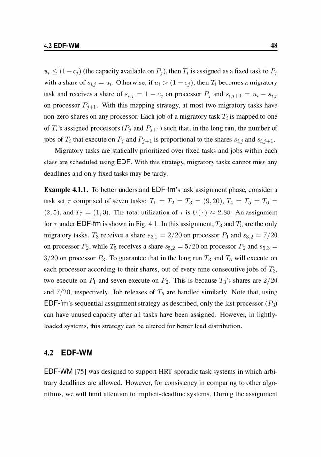
4.2 EDF-WM 48
ui ≤ (1− cj) (the capacity available on Pj), then Ti is assigned as a fixed task to Pjwith a share of si,j = ui. Otherwise, if ui > (1− cj), then Ti becomes a migratory
task and receives a share of si,j = 1 − cj on processor Pj and si,j+1 = ui − si,jon processor Pj+1. With this mapping strategy, at most two migratory tasks have
non-zero shares on any processor. Each job of a migratory task Ti is mapped to one
of Ti’s assigned processors (Pj and Pj+1) such that, in the long run, the number of
jobs of Ti that execute on Pj and Pj+1 is proportional to the shares si,j and si,j+1.
Migratory tasks are statically prioritized over fixed tasks and jobs within each
class are scheduled using EDF. With this strategy, migratory tasks cannot miss any
deadlines and only fixed tasks may be tardy.
Example 4.1.1. To better understand EDF-fm’s task assignment phase, consider a
task set τ comprised of seven tasks: T1 = T2 = T3 = (9, 20), T4 = T5 = T6 =
(2, 5), and T7 = (1, 3). The total utilization of τ is U(τ) ≈ 2.88. An assignment
for τ under EDF-fm is shown in Fig. 4.1. In this assignment, T3 and T5 are the only
migratory tasks. T3 receives a share s3,1 = 2/20 on processor P1 and s3,2 = 7/20
on processor P2, while T5 receives a share s5,2 = 5/20 on processor P2 and s5,3 =
3/20 on processor P3. To guarantee that in the long run T3 and T5 will execute on
each processor according to their shares, out of every nine consecutive jobs of T3,
two execute on P1 and seven execute on P2. This is because T3’s shares are 2/20
and 7/20, respectively. Job releases of T5 are handled similarly. Note that, using
EDF-fm’s sequential assignment strategy as described, only the last processor (P3)
can have unused capacity after all tasks have been assigned. However, in lightly-
loaded systems, this strategy can be altered for better load distribution.
4.2 EDF-WM
EDF-WM [75] was designed to support HRT sporadic task systems in which arbi-
trary deadlines are allowed. However, for consistency in comparing to other algo-
rithms, we will limit attention to implicit-deadline systems. During the assignment
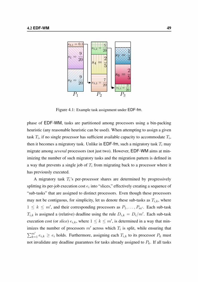
4.2 EDF-WM 49
s3,1 = 0.1
s2 =9
20
s1 =9
20
s5,2 =5
20
s4 =2
5
s3,2 =7
20s5,3 =
3
20
s6 =2
5
s7 =1
3
P1 P2 P3
Figure 4.1: Example task assignment under EDF-fm.
phase of EDF-WM, tasks are partitioned among processors using a bin-packing
heuristic (any reasonable heuristic can be used). When attempting to assign a given
task Ti, if no single processor has sufficient available capacity to accommodate Ti,
then it becomes a migratory task. Unlike in EDF-fm, such a migratory task Ti may
migrate among several processors (not just two). However, EDF-WM aims at min-
imizing the number of such migratory tasks and the migration pattern is defined in
a way that prevents a single job of Ti from migrating back to a processor where it
has previously executed.
A migratory task Ti’s per-processor shares are determined by progressively
splitting its per-job execution cost ei into “slices,” effectively creating a sequence of
“sub-tasks” that are assigned to distinct processors. Even though these processors
may not be contiguous, for simplicity, let us denote these sub-tasks as Ti,k, where
1 ≤ k ≤ m′, and their corresponding processors as P1, . . . , Pm′ . Each sub-task
Ti,k is assigned a (relative) deadline using the rule Di,k = Di/m′. Each sub-task
execution cost (or slice) ei,k, where 1 ≤ k ≤ m′, is determined in a way that min-
imizes the number of processors m′ across which Ti is split, while ensuring that∑m′
k=1 ei,k ≥ ei holds. Furthermore, assigning each Ti,k to its processor Pk must
not invalidate any deadline guarantees for tasks already assigned to Pk. If all tasks
4.2 EDF-WM 50
s2 =9
20
s1 =9
20
s4 =2
5
s3 =9
20 s5 =2
5
s6 =2
5
s7,3 = 0.167
P1 P2 P3
S7 =1
3
S7,2 = 0.144
123
S7,1 = 0.02
Figure 4.2: Example task assignment under EDF-WM.
in a task system τ can be successfully assigned (either completely or in a split way),
then τ is schedulable. Contrary to EDF-fm, the jobs of both fixed tasks and sub-
tasks on each processor are scheduled using EDF (no static prioritization). The
“job” of a sub-task Ti,k cannot execute before the corresponding “job” of the pre-
vious sub-task Ti,k−1 has finished execution. To enforce this precedence constraint,
EDF-WM assigns release times such that rji,k = rji,k−1 +Dji,k−1, where rji,k (rji,k−1)
is the release time of the j-th job of Ti,k (Ti,k−1), and Dji,k−1 is the relative deadline
of Ti,k−1.
Example 4.2.1. Fig. 4.2 shows an example task assignment (using the first-fit bin-
packing heuristic) for EDF-WM for the same task set of Example 4.1.1. In EDF-
WM, only task T7 = (1, 3) is migratory. Each job of T7 executes on processors
P3, P2, and P1 in sequence. For each sub-task T7,k of T7 (k ∈ {3, 2, 1}), D7,k =
D7/3 = 1.0. Assuming that the first job of the first sub-task of T7, T7,3, is released
on processor P3 at time 0, the first job of the sub-task T7,2 would be released on
P2 at time 1, and that of T7,1 at time 2 on P1. The shares assigned to each sub-
task are shown in the figure and correspond to execution times e7,3 = 0.5, e7,2 =
0.43, and e7,1 = 0.07. These execution times (which are determined during the
assignment phase) are computed in a way that ensures that no deadlines will be
4.3 NPS-F 51
missed (see [75]). Contrary to EDF-fm, more than one processor may have unused
capacity once all tasks have been assigned.
4.3 NPS-F
NPS-F [33, 34] was designed to schedule HRT implicit-deadline sporadic task sys-
tems. The algorithm employs a parameter δ that allows its utilization bound to be
increased at the cost of more-frequent preemptions. In comparison to earlier algo-
rithms [8, 32], NPS-F achieves a higher utilization bound, with a lower or compara-
ble preemption frequency. The assignment phase for NPS-F is a two-step process.
In the first step, the set of all n tasks is partitioned (using the first-fit heuristic) among
as many unit-capacity servers as needed. (A server in this context can be viewed as
a virtual uniprocessor.) Since n is finite and no tasks are split, the first step results
in the creation of m servers (for some m ∈ {1, . . . , n}). In the second step, the
capacity ci of each server Ni is increased by means of an inflation function I(δ, ci)
to ensure schedulability, i.e., a certain amount of over-provisioning is required to
avoid deadline misses. The m servers of inflated capacity I(δ, ci) (called notional
processors of fractional capacity—NPS-F—in [33]) are mapped onto the m physi-
cal processors of the platform. Such a mapping is feasible iff∑m
i=1 I(δ, ci) ≤ m.
The mapping of servers to physical processors is similar to the sequential as-
signment performed by EDF-fm: a server Ni is assigned to a processor Pj as long
as the capacity of Pj is not exhausted. The fraction of the capacity of Ni that does
not fit on Pj is assigned to Pj+1. A second mapping strategy is described in [33] as
well, but both yield identical schedulability bounds and, on our platform (which will
be described in Ch. 5), the one considered here reduces the number of cross-socket
server and task migrations.
During execution, each server Ni is selected to run every S time units, where S
is a time slot length that is inversely proportional to δ and dependent on the mini-
mum period of the task set. Whenever a server is selected for execution, it schedules

4.3 NPS-F 52
N4
s5 =2
5
s6 =2
5
s7 =1
3
s2 =9
20
s1 =9
20s3 =
9
20
s4 =2
5
N1 N2 N3
(a)
Inflated N1
Inflated N2
Inflated N3 Inf.N4
Inflated N1
Inflated N2
Inflated N3
P1
P2
P3 Inf.N4
S = 0.6 t(b)
Figure 4.3: Example task assignment under NPS-F for δ = 5 and S = 0.6. The arrowsin inset (b) denote that, in the first slot, N2 first executes on P2, then migrates to P1; at theend of the slot, it migrates back to P2 (similarly for N3). Execution requirements for theinflated servers are: N1 ≈ 0.55, N2 ≈ 0.52, N3 ≈ 0.50, and N4 ≈ 0.22.
(using uniprocessor EDF) the tasks assigned to it. Thus, abstractly, NPS-F is a two-
level hierarchical scheduler.
As noted earlier, there exists a clustered variant of NPS-F, denoted C-NPS-F,
that was designed to entirely eliminate off-chip server (and task) migrations. Con-
trary to NPS-F, in C-NPS-F the physical layout of the platform is already con-
sidered during the first step of the assignment phase, and therefore, off-chip server
(and task) migrations can be explicitly forbidden. Compared to NPS-F, the bin-
packing-related problem to be solved in C-NPS-F during the assignment phase is
harder (there are additional constraints at the server and cluster level), and therefore
the schedulable utilization of C-NPS-F is inferior to that of NPS-F.
Example 4.3.1. Fig. 4.3 illustrates the two steps of the NPS-F assignment process
using the task system τ from Example 4.1.1. Inset (a) depicts the assignment of
tasks to servers. m = 4 servers are sufficient to partition τ without splitting any
task. Before mapping the servers to physical processors, the capacity ci of each
serverNi is inflated using the function I . Then, the servers are sequentially mapped
(using their inflated capacities) onto the three physical processors P1–P3. As seen

4.4 Implementation Concerns 53
in the resulting mapping inset (b), N2 is split between P1 and P2, while N3 is split
between P2 and P3.
Inset (b) also shows how servers periodically execute. In this example, S = 0.6
(and δ = 5), so every 0.6 time units, the depicted server execution pattern repeats.
At time t = S = 0.6, server N2 migrates from processor P1 to processor P2, while
server N3 migrates to processor P3. Tasks T3 and T4 (assigned to N2), and T5 and
T6 (assigned to N3) also migrate with their respective servers. As in the EDF-fm
sequential assignment strategy, NPS-F’s mapping of servers to processors leaves
only the last processor (P3) with unallocated capacity after all servers have been
mapped.
4.4 Implementation Concerns
Timing and migration-related problems are the major issues that need to be ad-
dressed when implementing the semi-partitioned scheduling algorithms mentioned
above.
4.4.1 Timing Concerns
In each of the algorithms above, timers are needed in order to perform various
scheduling-related activities. For example, in EDF-WM, timers must be programmed
to precisely enforce sub-task execution costs, and in NPS-F, timers are needed to
execute servers periodically and to enforce their execution budgets. Furthermore, in
both EDF-fm and EDF-WM, timers must be programmed on remote CPUs in order
to guarantee that future job releases will occur on the correct processors. As noted
in Sec. 2.3, programming a timer on a remote CPU entails additional costs that must
be considered when checking schedulability.
A second timing concern is related to timer precision and the resolution of
time available within the OS. In theory, algorithms like EDF-WM and NPS-F
may reschedule tasks very frequently. For example, assuming 1 ms corresponds
4.4 Implementation Concerns 54
to one time unit, T7,1 needs to execute for 0.07 ms in Fig. 4.2, while, in Fig. 4.3,
the unused capacity (idle time) after N4 on processor P3 is 0.007 ms. In reality,
policing such small time intervals is not possible without incurring prohibitive over-
heads, and reasonable minimum interval lengths must be assumed. In Linux, even
if high-resolution timers are used, the very high resolutions needed in these exam-
ples would be difficult, if not impossible, to achieve. Furthermore, the execution of
timer-triggered events may be delayed by, for example, interrupt-disabled sections;
the exact enforcement of a strict interval of time is therefore not possible.
4.4.2 Migration-related Concerns
In theoretical analysis, it is common to assume that job migrations take zero time.
In practice, several activities (acquiring locks, making a scheduling decision, per-
forming a context switch, etc.) need to be performed before a job that is currently
executing on one CPU can be scheduled and executed on a different CPU. Such
activities have a cost. Furthermore, given the coarse-grained protection mecha-
nism of tasks and run queues explained in Sec. 2.3, when tasks may migrate as
part of the scheduling process, extra care must be taken in order to avoid inconsis-
tent scheduling decisions (e.g., scheduling a migrating task on two CPUs simulta-
neously). This problem is exacerbated in scheduling algorithms such as NPS-F,
where—by design—concurrent scheduling decisions are likely to happen. For ex-
ample, in Fig. 4.3 at time S = 0.6, P2 races with P1 to schedule tasks of N2, and
(at the same time) P3 races with P2 to schedule tasks of N3. To cope with this
problem, our LITMUSRT implementation of NPS-F and C-NPS-F delegates the
control of task migrations to the CPU that is currently executing the migrating task:
this CPU will inform the target CPU (using an IPI) when the migrating task has
become available for execution.

Chapter 5
Measuring Overheads
This chapter describes how kernel overheads and cache-related preemption and mi-
gration delays were determined on the platform employed in our experiments. In
Ch. 6, we report on multiprocessor EDF and semi-partitioned schedulability exper-
iments; in these experiments the overheads measured in this chapter are explicitly
accounted for.
After describing the hardware platform that was used in the experiments, we
detail the measurement process and experimental results of kernel overheads under
multiprocessor EDF algorithms and semi-partitioned algorithms implemented un-
der LITMUSRT (Sec. 3.3). We further present the two methodologies employed to
empirically assess CPMD, and we compare the results emerging from the applica-
tion of these methodologies on an experimental case study.
Hardware platform. Kernel overheads and preemption/migration delays detailed
in the following sections were measured in LITMUSRT on an Intel Xeon L7455
“Dunnington” system. The L7455 is a 24-core 64-bit uniform memory access
(UMA) machine with four physical sockets. Each socket contains six cores running
at 2.13 GHz. All cores in a socket share a unified 12-way set associative 12 MB L3
cache, while groups of two cores share a unified 12-way set associative 3 MB L2
cache. Each core also includes an 8-way set associative 32 KB L1 data cache and an
55
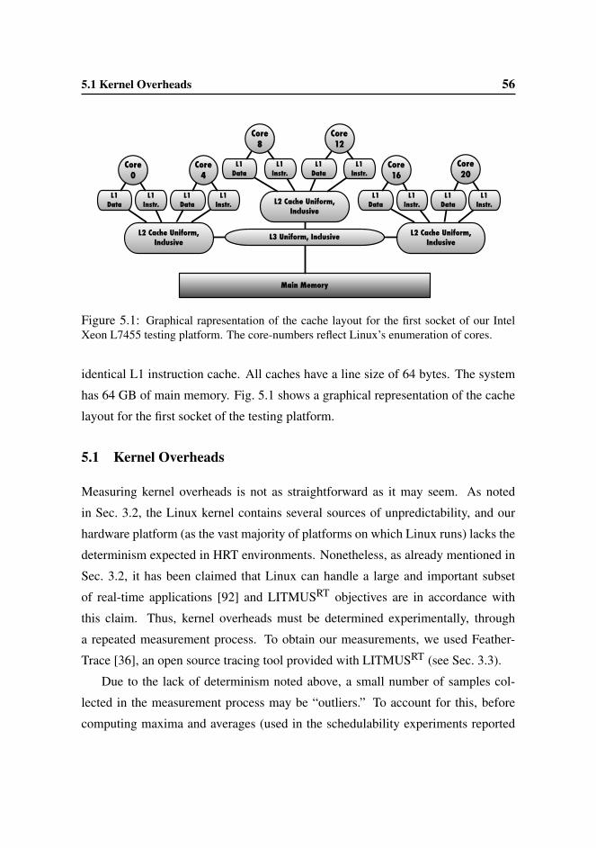
5.1 Kernel Overheads 56
Main Memory
L3 Uniform, Inclusive
L1 Data
Core 4
L2 Cache Uniform, Inclusive
L1 Instr.
L1 Data
Core 0
L1 Instr.
L1 Data
Core 12
L2 Cache Uniform, Inclusive
L1 Instr.
L1 Data
Core 8
L1 Instr.
L1 Data
Core 20
L2 Cache Uniform, Inclusive
L1 Instr.
L1 Data
Core 16
L1 Instr.
Figure 5.1: Graphical rapresentation of the cache layout for the first socket of our IntelXeon L7455 testing platform. The core-numbers reflect Linux’s enumeration of cores.
identical L1 instruction cache. All caches have a line size of 64 bytes. The system
has 64 GB of main memory. Fig. 5.1 shows a graphical representation of the cache
layout for the first socket of the testing platform.
5.1 Kernel Overheads
Measuring kernel overheads is not as straightforward as it may seem. As noted
in Sec. 3.2, the Linux kernel contains several sources of unpredictability, and our
hardware platform (as the vast majority of platforms on which Linux runs) lacks the
determinism expected in HRT environments. Nonetheless, as already mentioned in
Sec. 3.2, it has been claimed that Linux can handle a large and important subset
of real-time applications [92] and LITMUSRT objectives are in accordance with
this claim. Thus, kernel overheads must be determined experimentally, through
a repeated measurement process. To obtain our measurements, we used Feather-
Trace [36], an open source tracing tool provided with LITMUSRT (see Sec. 3.3).
Due to the lack of determinism noted above, a small number of samples col-
lected in the measurement process may be “outliers.” To account for this, before
computing maxima and averages (used in the schedulability experiments reported

5.1 Kernel Overheads 57
in Ch. 6), we applied a 1.5 interquartile range (IQR) outliers removal technique.
According to this technique, an outlier is a sample that falls more than 1.5 IQR be-
low the first quartile or above the third quartile. The National Institute of Standards
and Technology (NIST) [99] suggests the use of IQR as a standard technique for
removing outliers.
For each analyzed algorithm, we used monotonic piecewise linear interpolation
to derive upper bounds for each overhead as a function of the task set size. These
upper bounds were used in the schedulability experiments described in Ch. 6. For
the few overheads where the measurements did not reveal a conclusive trend, we
assumed a constant value equal to the maximum observed value.
5.1.1 Kernel Overheads under Multiprocessor EDF Algorithms
In the evaluation of P-EDF, G-EDF, and C-EDF, the three-level cache hierarchy of
our machine allowed us to set two cluster sizes for C-EDF. In the first configuration,
C-EDF-L2, cores are grouped around L2 caches and the platform is partitioned into
12 clusters of two cores each. The second configuration, C-EDF-L3, groups cores
around L3 caches, partitioning the platform into four six-core clusters.
For each algorithm, kernel overheads were obtained by measuring the system’s
behavior for periodic task sets. As G-EDF and P-EDF are a special case of C-EDF,
task sets were defined per-cluster, using a single cluster of size 24 for G-EDF, and
24 clusters of size one for P-EDF. Per-cluster task-set sizes were defined to range
over [10, 350] for G-EDF (task-set sizes are equal to the total number of tasks in
this case), over [1, 15] for P-EDF, over [3, 50] for C-EDF-L3, and over [1, 20]
for C-EDF-L2. The granularity of each range is defined by steps that were sized
variably to achieve higher resolution when the total number of tasks is at most 60
(the majority for task sets for the distributions presented in Sec. 6.3 have sizes in the
range [1,60]).
For each task-set size, we measured 10 task sets generated randomly with uni-
form light utilizations and moderate periods (see Sec. 6.2.1 for details on the ranges

5.1 Kernel Overheads 58
corresponding to light utilizations and moderate periods), for a total of 550 task sets.
We further verified that overheads measured using task sets generated with uniform
medium utilizations yielded similar results. Generated task sets are composed by
CPU-bound tasks that run (under the evaluated scheduling policy) according to their
generated parameters. To evaluate the impact of cache and memory accesses on ker-
nel overheads, each task reads and writes data from and to memory according to a
pre-specified pattern. Each task set was traced for 60 seconds. In total, more than
35 GB of trace data and 500 million individual overhead measurements where ob-
tained during more than 20 hours of tracing. After removing outliers as discussed
above, we computed average- and worst-case overheads for each plugin as a func-
tion of task-set size, which resulted in 12 graphs. In this section, we only discuss
the two representative graphs shown in Fig. 5.2, while a complete set of graphs for
all measured kernel overheads can be found in Appendix B.1 and in [23].
Inset (a) of Fig. 5.2 shows worst-case scheduling overheads (measured in µs)
as a function of the total number of tasks. The most notable trend here is the high
scheduling overhead (up to 200 µs) incurred by G-EDF compared to the overhead
experienced by C-EDF and P-EDF (less than 30 µs). Scheduling overhead for G-
EDF sharply increases with the number of tasks, as the contention and the length of
the global run queue increases. Such overhead is likely due to the cost of frequent
cache line migrations (“cache-line bouncing”) and heavy contention for the global
run-queue lock among all cores. Interestingly, scheduling overhead for the C-EDF
variants and P-EDF are similar.
Fig. 5.2 (b) shows worst-case release overheads as a function of the total number
of tasks. As before, G-EDF overhead is remarkably higher than those of the other
plugins. Again, this is mostly due to cache-line-bouncing effects and to the higher
contention for the global run queue. Interestingly, P-EDF overhead is markedly
lower than C-EDF overhead and C-EDF-L3 overhead is slightly more dependent
on the number of tasks.

5.1 Kernel Overheads 59
P-EDF C-EDF-L2 C-EDF-L3 G-EDF[1] [2] [3] [4]
0
50
100
150
200
250
0 50 100 150 200 250 300 350 400
over
head
(us
)
number of tasks
worst-case scheduling overhead
[4]
[3][2][1]
(a)
0
50
100
150
200
250
0 50 100 150 200 250 300 350 400
over
head
(us
)
number of tasks
worst-case release overhead
[4]
[3][1] [2]
(b)
Figure 5.2: Sample worst-case overhead measurements for P-EDF, G-EDF, C-EDF-L2,and C-EDF-L3. The graphs show worst-case measured overheads (in µs) as function oftask set size. (a) Scheduling overhead. (b) Release overhead. A complete set of graphs forall measured kernel overheads can be found in Appendix B.1.
5.1 Kernel Overheads 60
5.1.2 Kernel Overheads under Semi-Partitioned Algorithms
We measured kernel overheads incurred by tasks under semi-partitioned schedul-
ing algorithms using the same methodology presented above. In the evaluation of
semi-partitioned algorithms, for both assessing measured kernel overheads and an-
alyzing schedulability results (discussed in Sec. 6.4), we used P-EDF and C-EDF
as a basis for comparison. In fact, as shown in Sec. 6.3 and [25, 37, 39], P-EDF
proved to be very effective for HRT workloads, whereas C-EDF excelled at SRT
workloads. Under C-EDF, we opted to group cores around L3 caches (four clusters
of six cores each). This cluster size was selected based on the guidelines presented
in Sec. 6.3 and also discussed in [25, 45]. The same cluster size was also used for
C-NPS-F, as it yields the highest possible utilization bound given the topology of
our platform [33].
We traced workloads consisting of implicit-deadline periodic tasks under each
of the six evaluated algorithms (EDF-fm, EDF-WM, NPS-F, C-NPS-F, P-EDF,
and C-EDF). Task set sizes ranged over [10, 350] with a granularity of 10 in the
range [10, 200], and 50 in the range (200, 350]. These granularities allow for a
higher resolution when the number of tasks is less than 200 (which is the prevalent
range of task set sizes for the distributions presented in Sec. 6.4). For each task set
size, we measured ten randomly generated task sets (with uniform light utilizations
and moderate periods; see Secs. 6.2.1). As in Sec. 5.1.1, generated task sets are
composed by CPU-bound tasks that run according to their generated parameters.
To evaluate the impact of cache and memory accesses on kernel overheads, each
task reads and writes data from and to memory according to a pre-specified pattern.
Each task set was traced for 60 seconds. Due to the timing concerns mentioned in
Sec. 4.4, we enforced a minimum sub-task execution cost of 50 µs under EDF-WM,
and imposed a minimum server size of 150 µs under NPS-F to allow some room
for tasks to execute within their servers. We further used task sets with S ≥ 2.5 ms
(and δ = 2) to limit the number of server-switches.

5.2 Cache-Related Delays 61
In total, more than 1,300 task sets were traced, and more than 200 GB of over-
head samples were collected. In Appendix C.1 and in the extended version of [26],
this overhead data is given in 14 graphs; similarly to Sec. 5.1.1, in this section only
the two representative graphs plotted in Fig. 5.3 are discussed.
Fig. 5.3(a) shows worst-case scheduling overheads (measured in µs) as a func-
tion of the total number of tasks, while Fig. 5.3(b) shows worst-case release over-
heads as a function of the total number of tasks. The most notable trends in both
insets (and particularly in Fig. 5.3(b)) are the higher overheads of C-EDF in com-
parison with the other algorithms, and the low overheads (within 5 – 10 µs from
P-EDF) of all semi-partitioned algorithms. Under semi-partitioned approaches, mi-
grations are push-based: semi-partitioned algorithms statically determine the next
processor that should schedule a job (i.e., the job is “pushed” to the processor where
it should execute next when it finishes execution on the previous processor). In-
stead, under C-EDF (and under global approaches), migrations are pull-based: the
next processor is dynamically determined at runtime (the job is “pulled” by the
processor that dequeues it first from the run queue). Pull-migrations imply much
higher overheads as they require global state and shared run queues that foster lock
contention, which is reflected in Fig. 5.3. Instead, push-migrations yield lower over-
heads as most state-updates are local within per-CPU run queues, thus reducing lock
contention for shared run queues.
5.2 Cache-Related Delays
In this section, we describe the general setup and the two methodologies developed
to empirically approximate cache-related delays. We also present (Sec. 5.2.2) a case
study where the results of the two methodologies are compared and discussed. We
conclude this section with the interpretation of relevant observations arising from
results of the case study.

5.2 Cache-Related Delays 62
C-EDF C-NPS-F EDF-fm EDF-WM NPS-F P-EDF[1] [2] [3] [4] [5] [6]
0
5
10
15
20
25
30
0 50 100 150 200 250 300 350number of tasks
worst-case scheduling overhead
over
head
(us)
[1]
[2][3]
[4]
[6]
[5]
(a)
0
5
10
15
20
25
30
35
40
0 50 100 150 200 250 300 350
over
head
(us)
number of tasks
worst-case release overhead
[1]
[2, 3, 4, 5]
[6]
(b)
Figure 5.3: Sample worst-case overhead measurements under P-EDF, C-EDF, EDF-fm,EDF-WM, NPS-F, and C-NPS-F. The graphs show worst-case measured overheads (inµs) as function of task set size. (a) Scheduling overhead. (b) Release overhead. A completeset of graphs for all measured kernel overheads can be found in Appendix C.1.

5.2 Cache-Related Delays 63
T ji
t
t0
Cold
t1
Warm
t2 t3
Preemption
t4
After Preempt.
t5
Warm Delay
1
Figure 5.4: Cache-delay measurement.
5.2.1 Measuring Cache-Related Preemption and Migration Delays
Recall that a job is delayed after a preemption or a migration due to a (partial) loss
of cache affinity. To measure such delays, we consider jobs that access their WS as
illustrated in Fig. 5.4: a job T ji starts executing cache-cold at time t0 and experiences
compulsory misses until time t1, when its WS is completely loaded into cache. After
t1, each subsequent memory reference by T ji is cache-warm. At time t2, the job has
successfully referenced its entire WS in a cache-warm context. From t2 onward,
the job repeatedly accesses single words of its WS (to maintain cache affinity) and
checks after each access if a preemption or migration has occurred. Suppose that the
job is preempted at time t3 and not scheduled until time t4. As T ji lost cache affinity
during the interval [t3, t4], the length of the interval [t4, t5] (i.e., the time needed to
reference again its entire WS) reflects the time lost to additional cache misses.
Let dc denote the cache-related delay suffered by T ji . After the WS has been
fully accessed for the third time (at time t5), dc is given by the difference dc =
(t5− t4)− (t2− t1). (The interval [t2, t3] is not reflected in dc since jobs are simply
waiting to be preempted while maintaining cache affinity during this interval.) After
collecting a trace of samples dc,0, dc,1, . . . , dc,k from a sufficiently large number of
jobs k, maxl{dc,l} can be used to approximate D, the bound on the maximum
CPMD incurred by any job. Similarly, average delay and standard deviation can be
5.2 Cache-Related Delays 64
readily computed from such a trace during off-line analysis.
On multiprocessors with a hierarchy of shared caches, migrations are catego-
rized according to the level of cache affinity that is preserved (e.g., a job migration
between two processors sharing an L2 cache is an L2-migration). A memory migra-
tion does not preserve any level of cache affinity. Migrations can be identified by
recording at time t3 the processor P on which T ji was executing and at time t4 the
processor R on which T ji resumes execution.
Each sample dc,l can be obtained either directly or indirectly. A low-overhead
clock device can be used to directly measure the WS access times [t1, t2] and [t4, t5],
which immediately yield dc. Alternatively, some platforms include hardware per-
formance counters that can be used to indirectly measure dc by recording the num-
ber of cache misses. The number of cache misses experienced in each interval is
then multiplied by the time needed to service a single cache miss. Here, we focus
on the direct measure of WS access times, as reliable and precise clock devices
are present on virtually all (embedded) platforms. In contrast, the availability of
suitable performance counters varies greatly among platforms.
Cache-related preemption and migration delays clearly depend on the WSS of
a job and possibly on the scheduling policy [39] and on the task set size (TSS).
Hence, to detect such dependencies (if any), each trace dc,0, dc,1, . . . , dc,k should
ideally be collected on-line, i.e., as part of a task set that is executing under the
scheduler that is being evaluated without altering the implemented policy. We next
describe a method that realizes this idea.
Schedule-Sensitive Method
With this method, the dc samples are recorded on-line while scheduling task sets
under the algorithm of interest. Performing these measurements without changing
the regular scheduling of a task set poses the question of how to efficiently distin-
guish between a cold, warm, and post-preemption (or migration — post-pm) WS
access. In particular, detecting a post-pm WS access is subtle, as jobs running un-

5.2 Cache-Related Delays 65
der OSs with address space separation (e.g., Linux) are generally not aware of being
preempted or migrated. Solving this issue requires a low-overhead mechanism that
allows the kernel to inform a job of every preemption and migration. Note that the
schedule-sensitive method crucially depends on the presence of such a mechanism
(a suitable implementation is presented in Sec. 5.2.1 below).
Delays should be recorded by executing test cases with a wide range of TSSs
and WSSs. This likely results in traces with a variable number of valid samples. To
obtain an unbiased estimator for the maximum delay, the same number of samples
should be used in the analysis of each trace. In practice, this implies that only (the
first) kmin from each trace can be used, where kmin is the minimum number of valid
samples among all traces.
Since samples are collected from a valid schedule, the advantage of this method
is that it can identify dependencies (if any) of CPMD on scheduling decisions and
on the number of tasks. However, this implies that it is not possible to control when
a preemption or a migration will happen, since these decisions depend exclusively
on the scheduling algorithm (which is not altered). Therefore, the vast majority of
the collected samples are likely invalid, e.g., a job may not be preempted at all or
may be preempted prematurely, and only samples from jobs that execute exactly as
shown in Fig. 5.4 can be used in the analysis. Thus, large traces are required to
obtain few samples. Worse, for a given scheduling algorithm, not all combinations
of WSS and TSS may be able to produce the execution pattern needed in the analysis
(e.g., this is the case with G-EDF, as discussed in Sec. 5.2.2).
Hence, we developed a second method that achieves finer control over the mea-
surement process by artificially triggering preemptions and migrations of a single
task.
Synthetic Method
In this approach, CPMD measures are collected by a single task that repeatedly ac-
cesses WSs of different sizes. The task is assigned the highest priority and therefore
5.2 Cache-Related Delays 66
it cannot be preempted by other tasks.
In contrast to the schedule-sensitive method, preemptions and migrations are ex-
plicitly triggered in the synthetic method. In particular, the destination core and the
preemption length are chosen randomly (preemptions arise if the same core is cho-
sen twice in a row). In order to trigger preemptions, L2-migrations, L3-migrations,
etc. with the same frequency (and thus to obtain an equal number of samples),
proper probabilities must be assigned to each core. Furthermore, as the task execu-
tion is tightly controlled, post-pm WS accesses do not need to be detected, and no
kernel interaction is needed.
The synthetic method avoids the major drawback of the previous approach, as
it generates only valid post-pm data samples. This allows a statistically meaning-
ful number of samples to be obtained rapidly. However, as preemption and migra-
tion scheduling decision are externally imposed, this methodology cannot determine
possible dependencies of CPMD on scheduling decisions or on the TSS.
Implementation Concerns
Both methods were implemented using version 2010.1 of LITMUSRT, which is
based on Linux 2.6.32.
Precise time measures of WS access times were obtained on the x86 Intel plat-
form used in our experiments (see Ch. 5) by means of the time-stamp counter (TSC),
a per-core counter that can be used as high-resolution clock device. The direct mea-
sure of CPMD on a multiprocessor platform should take into account the imperfect
alignment of per-processor clock devices (clock skew). Clock skew errors can be
avoided if WS access times are evaluated only based on samples obtained on the
same processor (e.g., in Fig. 5.4, t1 and t2 should be measured on the same pro-
cessor, which may differ from the processor where t4 and t5 are measured).1 In
addition, to improve the predictability of our measures and to avoid the impact of1Since measured CPMDs are in the micro- and milli-second ranges, the impact of clock drift due
to (small) clock skew errors is limited.

5.2 Cache-Related Delays 67
power saving policies on the TSC (power saving policies may dynamically modify
the CPU frequency, and thus TSC resolution), we disabled cache-line prefetching
and we disabled power management and frequency scaling.
In most OSs, time interval measurements can be further perturbed by interrupt
handling. These disturbances can be avoided by disabling interrupts while mea-
suring WS access times. Although this does not prevent non-maskable interrupts
(NMIs) from being serviced, NMIs are infrequent events that likely only have a
minor impact on CPMD approximations. We note, however, that our methodology
currently cannot detect interference from NMIs.
Disabling interrupts under the schedule-sensitive method is a tradeoff between
accuracy and the rate at which samples are collected. On the one hand, disabling
interrupts increases the number of valid samples, but on the other hand, it implicitly
alters the scheduling policy by introducing non-preemptive sections. We chose to
disable interrupts to reduce the length of the experiments.
Within LITMUSRT, we implemented the low-overhead kernelspace–userspace
communication mechanism required by the schedule-sensitive method by sharing a
single per-task memory page (the control page) between the kernel and each task. A
task can infer whether it has been preempted or migrated based on the control page:
when it is selected for execution, the kernel updates the task’s control page by in-
creasing a preemption counter and the job sequence number, storing the preemption
length, and recording on which core the task will start its execution.
Given our empirical methods to measure delays, computing maxima and av-
erages needs some observations. In the schedule-sensitive method, each post-pm
sample does not represent the main behavior of the system, but the behavior of
infrequent carefully-selected events among several WSS accesses. These post-pm
samples may be wrongly considered as outliers by outliers removal techniques such
as the IRQ technique employed in Sec. 5.1. Therefore, we considered all these post-
pm samples as valid samples. However, for a given WSS, the number of collected

5.2 Cache-Related Delays 68
preemption and migration samples for different TSSs may change.2 To evaluate
statistics on a non-biased sample set for each type of overhead measure, we reduced
the number samples used to compute each preemption/migration type statistic, to
the minimum number of samples (per preemption/migration types) recorded among
all TSS.
The synthetic method allows to collect a high number of samples that present the
desired WSS access pattern. Visual inspection revealed that these samples are prac-
tically not affected by unpredictabilities related to interrupt management. Therefore,
we consider all samples to be valid for this method, too.
5.2.2 Evaluation
To verify and compare results of the two presented methods, we measured CPMDs
using both methodologies on the testing platform described at the beginning of this
chapter.
Experimental Setup
We used the G-EDF algorithm to measure CPMD with the schedule-sensitive method,
but we emphasize that the method can be applied to other algorithms as well. For
this method, we measured the system behavior of periodic task sets consisting of
25 to 250 tasks in steps of variable sizes (from 20 to 30, with smaller steps where
we desired a higher resolution). Task WSSs were varied over {4, 32, 64, . . . , 2048}KB. Per-WSS write ratios of 1/2 and 1/4 were assessed. In preliminary tests with
different write ratios, 1/2 and 1/4 showed the highest worst-case overheads, with
1/4 performing slightly worse. All write ratios are given with respect to individual
words, not cache lines. There are eight words in each cache line, thus each task up-
dated every cache line in its WS multiple times. Tests with write ratios lower than
1/8, under which some cache lines are only read, exhibited reduced overheads. For2In the schedule-sensitive method, the occurrence of valid post-pm samples cannot be explicitly
controlled and depends on the scheduling decisions taken by the employed scheduling algorithm.
5.2 Cache-Related Delays 69
each WSS and TSS, we measured ten randomly-generated task sets using parameter
ranges from [37, 39]. Each task set was traced for 60 seconds and each experiment
was carried out once in an otherwise idle system and once in a system loaded with
best-effort cache-polluter tasks. Each of these tasks was statically assigned to a core
and continuously thrashed the L1, L2, and L3 caches by accessing large arrays.
In total, more than 50 GB of trace data with 600 million overhead samples were
obtained during more than 24 hours of tracing.
We used a single SCHED FIFO task running at the highest priority to measure
CPMD with the synthetic method. The WSS was chosen from {4, 8, 16, . . . , 8192}KB. We further tested WSSs of 3 and 12 MB, as they correspond to the sizes of the
L2 and L3 cache respectively. In these experiments, several per-WSS write ratios
were used. In particular, we considered write ratios ranging over {0, 1/128, 1/64,
1/16, 1/4, 1/2, 1}. For each WSS we ran the test program until 5,000 valid after-
pm samples were collected (for each preemption/migration category). Preemption
lengths were uniformly distributed in [0ms, 50ms]. As with the schedule-sensitive
method, experiments were repeated in an idle system and in a system loaded with
best-effort cache-polluter tasks. More than 3.5 million valid samples were obtained
during more than 50 hours of tracing.
Results
Fig. 5.5 and Fig. 5.6 show preemption and migration delays that were measured
using the synthetic method (the data is given numerically in Appendix A). In both
figures, each inset indicates CPMD values for preemptions and all different kinds
of migrations (L2, L3, memory) as a function of WSS, assuming a write ratio of
1/4. Fig. 5.5(a) and Fig. 5.6(a) give delays obtained when the system was loaded
with cache-polluter tasks, while Fig. 5.5(b) and Fig. 5.6(b) give results that were
recorded in an otherwise idle system. Fig. 5.5 presents worst-case overheads, and
Fig. 5.6 shows average overheads; the error bars depict one standard deviation. In
all graphs, both axes are in logarithmic scale. Note that these graphs display the

5.2 Cache-Related Delays 70
600
800
1000
1200
1400
1600
1800
2000
2200
2400
60 80 100 120 140 160 180 200 220 240 260
over
head
(us
)
number of tasks
measured maximum overhead (25.00% writes)
a preemptiona migration through a shared L2 cache
a migration through a shared L3 cachea migration through main memory
10
100
1000
10000
100000
4 16 64 256 1024 4096 16384
cach
e-re
late
d de
lays
(us
)
working set size (kilobytes)
measured maximum overhead (25.00% writes)
(a)
0.1
1
10
100
1000
10000
4 16 64 256 1024 4096 16384
cach
e-re
late
d de
lays
(us
)
working set size (kilobytes)
measured maximum overhead (25.00% writes)
(b)
Figure 5.5: CPMD approximations obtained with the synthetic method. The graphs showmaximum CPMD (in µs) for preemptions and different types of migrations as a function ofWSS (in KB). (a) Worst-case delay under load. (b) Worst-case delay in an idle system.
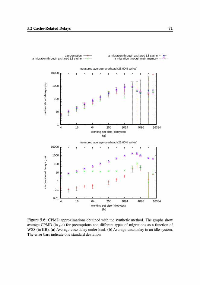
5.2 Cache-Related Delays 71
600
800
1000
1200
1400
1600
1800
2000
2200
2400
60 80 100 120 140 160 180 200 220 240 260
over
head
(us
)
number of tasks
measured maximum overhead (25.00% writes)
a preemptiona migration through a shared L2 cache
a migration through a shared L3 cachea migration through main memory
1
10
100
1000
10000
4 16 64 256 1024 4096 16384
cach
e-re
late
d de
lays
(us
)
working set size (kilobytes)
measured average overhead (25.00% writes)
(a)
0.01
0.1
1
10
100
1000
10000
4 16 64 256 1024 4096 16384
cach
e-re
late
d de
lays
(us
)
working set size (kilobytes)
measured average overhead (25.00% writes)
(b)
Figure 5.6: CPMD approximations obtained with the synthetic method. The graphs showaverage CPMD (in µs) for preemptions and different types of migrations as a function ofWSS (in KB). (a) Average-case delay under load. (b) Average-case delay in an idle system.The error bars indicate one standard deviation.

5.2 Cache-Related Delays 72
difference between a post-pm and a cache-warm WS access. Therefore, declining
trends with increasing WSSs (Fig. 5.5(b), Fig. 5.6(a,b)) indicate that the cache-warm
WS access cost is increasing more rapidly than the post-pm WS access.
Observation 5.2.1. The predictability of overhead measures is heavily influenced
by the size of L1 and L2 caches. This can be seen in Fig. 5.6(a): as the WSS
approaches the size of the L2 cache (3072 KB, shared among 2 cores), the standard
deviation of average delays becomes very large (the same magnitude of the measure
itself) and therefore overhead estimates are very imprecise. This unpredictability
arises because jobs with large WSSs suffer frequent L2- and L3-cache misses in a
system under load due to thrashing and cache interference, and thus become exposed
to memory bus contention. Due to the thrashing cache-polluter tasks, bus access
times are highly unpredictable and L3 cache interference is very pronounced. In
fact, our traces show that jobs frequently incur “negative CPMD” in such cases
because the “cache-warm” access itself is strongly interfered with. This implies
that, from the point of view of schedulability analysis, CPMD is not well-defined
for such WSSs, since a true WCET must account for worst-case cache interference
and thus is already more pessimistic than CPMD, i.e., actual CPMD effects are
likely negligible compared to the required bounds on worst-case interference.
Observation 5.2.2. In a system under load, there are no substantial differences
between preemption and migration costs, both in the case of worst-case (Fig. 5.5(a))
and average-case (Fig. 5.6(a)) delays. When a job is preempted or migrated in the
presence of heavy background activity, its cache lines are likely evicted quickly
from all caches and thus virtually every post-pm access reflects the high overhead
of refetching the entire WS from memory. Fig. 5.5(a) shows that, in a system under
load, the worst-case delay for a 256 KB WSS exceeds 1ms, while the cost for a
1024 KB WSS is around 5ms. Average-case delays (Fig. 5.6(a)) are much lower,
but still around 1ms for a 1024 KB WSS.
Observation 5.2.3. In an idle system, preemptions always cause less delay than

5.2 Cache-Related Delays 73
migrations, whereas L3- and memory migrations have comparable costs. This be-
havior can be observed in Fig. 5.5(b) and Fig. 5.6(b). In particular, if the WS fits
into the L1 cache (32 KB), then preemptions are negligible (around 1µs), while
they have a cost that is comparable with that of an L2 migration when the WSS
approaches the size of the L2 cache (still, they remain less than 1ms). Fig. 5.6(b)
clearly shows that L2 migrations cause less delay than L3 migrations for WSSs
that exceed the L1 cache size (about 10µs for WSSs between 32 and 1024 KB).
In contrast, L3 and memory migrations have comparable costs, with a maximum
around 3ms with 3072 KB WSS (Fig. 5.5(b)). Interestingly, memory migrations
cause slightly less delay than L3 cache migrations. As detailed below, this is most
likely related to the cache consistency protocol.
Observation 5.2.4. The magnitude of CPMD is strongly related to preemption
length (unless cache affinity is lost completely, i.e., in the case of memory migra-
tions). This trend is apparent from the plots displayed in Fig. 5.7. Inset (a) shows in-
dividual preemption delay measurements arranged by increasing preemption length,
inset (b) similarly shows L3 migration delay. The samples were collected using the
synthetic method with a 64 KB WSS and a write ratio of 1/4 in a system under load
(similar trends were observed with all WSSs ≤ 3072 KB). In both insets, CPMD
converges to around 50µs for preemption lengths exceeding 10ms. This value is
the delay experienced by a job when its WSS is reloaded entirely from memory. In
contrast, for preemption lengths ranging in [0ms, 10ms], average preemption de-
lay increases with preemption length (inset (a)), while L3 migrations (in the range
[0ms, 5ms]) progressively decrease in magnitude (inset (b)). The observed L3 mi-
gration trend is due to the cache consistency protocol: if a job resumes quickly after
being migrated, parts of its WS are still present in previously-used caches and thus
need to be evicted. In fact, if the job does not update its WS (i.e., if the write ratio
is 0), then the trend is not present.
L2 migrations (Fig. 5.8(a)) reveal a trend that is similar to the preemption case,

5.2 Cache-Related Delays 74
0 25 50 75
100 125 150 175 200 225 250 275
0 3000 6000 9000 12000 15000 18000 21000 24000
cach
e-re
late
d de
lay
(us)
preemption length (us)
post-preemption samples (WSS=64kB, 25% writes)
(a)
0 25 50 75
100 125 150 175 200 225 250 275
0 3000 6000 9000 12000 15000 18000 21000 24000
cach
e-re
late
d de
lay
(us)
preemption length (us)
post-L3-migration samples (WSS=64kB, 25% writes)
(b)
Figure 5.7: Scatter plot of observed dc samples vs. preemption length in a system underload. (a) Samples recorded after a preemption. (b) Samples recorded after an L3-migration.The plots have been truncated at 25ms; there are no trends apparent in the range from 25msto 50ms.
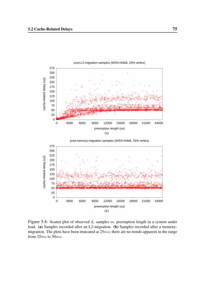
5.2 Cache-Related Delays 75
0 25 50 75
100 125 150 175 200 225 250 275
0 3000 6000 9000 12000 15000 18000 21000 24000
cach
e-re
late
d de
lay
(us)
preemption length (us)
post-L2-migration samples (WSS=64kB, 25% writes)
(a)
0 25 50 75
100 125 150 175 200 225 250 275
0 3000 6000 9000 12000 15000 18000 21000 24000
cach
e-re
late
d de
lay
(us)
preemption length (us)
post-memory-migration samples (WSS=64kB, 25% writes)
(b)
Figure 5.8: Scatter plot of observed dc samples vs. preemption length in a system underload. (a) Samples recorded after an L2-migration. (b) Samples recorded after a memory-migration. The plots have been truncated at 25ms; there are no trends apparent in the rangefrom 25ms to 50ms.

5.2 Cache-Related Delays 76 600
800
1000
1200
1400
1600
1800
2000
2200
2400
60 80 100 120 140 160 180 200 220 240 260
over
head
(us)
number of tasks
measured maximum overhead (25.00% writes)
a preemptiona migration through a shared L2 cache
a migration through a shared L3 cachea migration through main memory
600
800
1000
1200
1400
1600
1800
2000
2200
2400
60 80 100 120 140 160 180 200 220 240 260
over
head
(us)
number of tasks
measured maximum overhead (25.00% writes)
a preemptiona migration through a shared L2 cache
a migration through a shared L3 cachea migration through main memory
500
1000
1500
2000
2500
3000
3500
4000
4500
5000
5500
60 80 100 120 140 160 180 200 220 240 260
cach
e-re
late
d de
lay
(us)
number of tasks
measured maximum overhead (25.00% writes)
Figure 5.9: Worst-case CPMD approximations as function of TSS in a system under load(obtained with the schedule-sensitive method). Lines are grouped by WSS: from top: WSS= 1024 KB, WSS = 512 KB, WSS = 256 KB.
while memory migrations (Fig. 5.8(b)) do not show a trend (samples are clustered
around 50µs delay regardless of preemption length).
Observation 5.2.5. Preemption and migration delays do not depend significantly on
the task set size. This can be observed in Fig. 5.9, which depicts worst-case delay
for the schedule-sensitive method in a system under load as function of TSS. The
plot indicates CPMD for preemptions and all migration types for WSSs of 1024,
512 and 256 KB (from top to bottom).
Note that Fig. 5.9 is restricted to TSSs from 75 to 250 because, under G-EDF,
only few task migrations occur for small TSSs (see Sec. 5.2.1). Thus, the number
of collected valid delays for small TSSs is not statistically meaningful.
Furthermore, Fig. 5.9 shows that worst-case preemption and migrations delays
for the same WSS have comparable magnitudes, thus confirming that, in a sys-
tem under load, preemption and migration costs do not differ substantially (recall

5.2 Cache-Related Delays 77
Fig. 5.5(a) and Observation 5.2.2).
Interpretation. The setup used in the experiments depicted in Fig. 5.5(a) and
Fig. 5.6(a), simulate worst-case scenarios in which a job is preempted by a higher-
priority job with a large WSS that (almost) completely evicts the preempted job’s
WS while activity on other processors generates significant memory bus contention.
In contrast, Fig. 5.5(b) and Fig. 5.6(b) correspond to situations in which the pre-
empting job does not cause many evictions (which is the case if it has a virtually
empty WS or its WS is already cached) and the rest of the system is idle, i.e.,
Fig. 5.5(b) and Fig. 5.6(b) depict best-case scenarios. Hence, Fig. 5.5(a) (resp.,
Fig. 5.6(a)) shows the observed worst-case (resp., average) cost of reestablishing
cache affinity in a worst-case situation, whereas Fig. 5.5(b) (resp., Fig. 5.6(b)) shows
the worst-case (resp., average) cost of reestablishing cache affinity in a best-case sit-
uation.
Further note that, even though the synthetic method relies on a background
workload to generate memory bus contention, the data shown in Fig. 5.5(a) and
Fig. 5.6(a) also applies to scenarios where the background workload is absent if the
real-time workload itself generates significant memory bus contention.
This has profound implications for empirical comparisons of schedulers. If it is
possible that a job’s WS is completely evicted by an “unlucky” preemption, then this
(possibly unlikely) event must be reflected in the employed schedulability test(s).
Thus, unless it can be shown (or assumed) that all tasks have only small WSSs and
there is no background workload (including background OS activity), then bounds
on CPMD should be estimated based on the high-contention scenario depicted in
Fig. 5.5(a) and Fig. 5.6(a).
Therefore, based on our data, it is not warranted to consider migrations to be
more costly than preemptions when making worst-case assumptions (e.g., when
applying HRT schedulability tests). Further, unless memory bus contention is guar-
anteed to be absent, this is the case even when using average case overheads (e.g.,

5.2 Cache-Related Delays 78
when applying SRT schedulability tests).

Chapter 6
Experimental Evaluation of Multiprocessor Sched-
uling Algorithms
In this chapter, we present and discuss the results of the comparison of multipro-
cessor EDF scheduling policies (P-EDF, G-EDF, and C-EDF) and of the compar-
ison of semi-partitioned scheduling algorithms (EDF-fm, EDF-WM, NPS-F, and
C-NPS-F). Relative performance of the evaluated algorithms are based on schedu-
lability (see. Sec. 2.2), i.e., on the ability of each algorithm to ensure timing con-
straints for sporadic task sets on our testing platform (which is described in Ch. 5).
In the experiments that follow, kernel overheads and cache-related delays as mea-
sured in Ch. 5 are explicitly considered.
In this chapter, we first discuss how system overheads and cache-related over-
heads can be accounted for in the schedulability analysis and we detail the spe-
cial considerations that are needed when accounting for overheads under semi-
partitioned algorithms. Afterwards, we describe the methodology employed in the
comparisons and we introduce our performance metrics. Finally, we discuss the
results of our evaluation.
79

6.1 Accounting for Overheads 80
6.1 Accounting for Overheads
Schedulability analysis that assumes ideal (i.e., without overheads) event-driven
scheduling can be extended to account for runtime overheads and cache-related pre-
emption and migration delays by inflating task execution costs.
Overheads that occur before or after a job is scheduled can be accounted for by
extending the job’s execution. A job T ji incurs two scheduling and two context-
switching overheads [85] and two preemption/migration overhead (one to account
for the lack of cache affinity at the beginning of T ji ’s execution, and one to account
for the cost of disrupting the cache affinity of the job preempted by T ji ). Similar
inflation can be done for IPI latencies and a job’s own release overhead. Instead, ac-
counting for overheads (release and timer-transfer overheads) that are due to other
jobs and for tick overheads is more complicated. While the general idea of inflating
job execution costs to account for overheads is conceptually simple, inflating cor-
rectly is challenging. A detailed survey of such overhead accounting techniques can
be found in several previous studies (e.g., [25, 37, 39, 40, 53]).
These standard techniques can be applied without changes to account for over-
heads in multiprocessor EDF scheduling algorithms, and for many of the overheads
considered under semi-partitioned scheduling algorithms. However, under semi-
partitioned scheduling policies, specific properties of these algorithms have to be
accounted for. For example, as semi-partitioned approaches distinguish between
migratory and fixed tasks, migration and preemption overheads always need to be
separately considered. Further, additional IPI latencies have to be accounted for in
EDF-WM to reflect the operations performed to guarantee sub-task precedence con-
straints, and in NPS-F to ensure consistent scheduling decisions when switching be-
tween servers (which occurs when the fraction of a timeslot allocated to one server
is exhausted and another server continues). In addition, NPS-F’s server-switching
imposes an additional overhead on all tasks executed within a server. These over-
heads can be accounted for by reducing the effective server capacity available to

6.1 Accounting for Overheads 81
tasks.
Bin-packing issues under semi-partitioning. In all of the evaluated semi-parti-
tioned algorithms, problematic issues (that we were the first to address in [26]) arise
when accounting for overheads during the assignment phase. Standard bin-packing
heuristics assume that item sizes (i.e., task utilizations) are constant. However, when
overheads are accounted for, the effective utilization of already-assigned tasks may
inflate when an additional task is added to their partition (i.e., bin) due to an in-
crease in overheads. Thus, ignoring overheads when assigning tasks may cause
over-utilization. To deal with this, we accounted for overheads after each task as-
signment and extended prior bin-packing heuristics to allow “rolling back” to the
last task assignment if the current one causes over-utilization. Without these exten-
sions, any task set exceeding the capacity of one processor would be unschedulable
by the commonly-used next-fit, best-fit, and first-fit heuristics (which try to fully
utilize one processor before considering others). In contrast, the worst-fit heuristic
(used in [25, 37, 39, 70]) partially hides this problem since it tends to distribute
unallocated capacity evenly among processors.
Considering overheads in the assignment phase of NPS-F exposes an addi-
tional issue that was not considered by the designers of that algorithm. If over-
heads are only accounted for after the mapping of servers to physical processors,
then a server’s allocation may grow beyond the slot length S. This would render
the mapping unschedulable, as it would essentially require servers and tasks to be
simultaneously scheduled on two processors. However, if overheads are already ac-
counted for during the first bin-packing phase, i.e., before the mapping to physical
processors, then it is unknown which servers (and hence tasks) will be migratory.
We resolve this circular dependency by making worst-case assumptions with regard
to the magnitude of overheads during the first bin-packing phase. Particularly, dur-
ing this phase, we consider each job as if it were a migrating job (and we account
for overheads accordingly). In the second phase, when the actual physical assign-

6.2 Schedulability Experiments 82
ment occurs, we recompute the overheads and we remove the additional pessimism.
Nonetheless, this approach adds pessimism during the first phase, but it is required
to prevent servers from becoming overloaded.
6.2 Schedulability Experiments
Recall that an algorithm’s schedulability (HRT or SRT) is defined as the fraction
of task sets that are schedulable (HRT or SRT) under it. In the real-time literature,
comparisons on the basis of schedulability have been widely used. Particularly, in
our investigations we seek to identify which of the considered algorithms is more
likely to successfully schedule a given workload when system overheads are con-
sidered.
6.2.1 Task Set Generation
The core of a schedulability study is a parametrized task set generation procedure
that is used to repeatedly create (and test) task sets while varying the parameters over
their respective domains. When creating a task set τ , such procedure determines the
number of tasks n in τ and each task Ti’s execution time ei and period pi. In both the
evaluation of multiprocessor EDF schedulers and semi-partitioned schedulers, we
generated implicit-deadline periodic tasks employing an experimental setup similar
to previous studies [37, 39, 46]. In our experiments, the generation procedures use
distributions that are similar to those proposed by Baker in [18].
In the comparison of multiprocessor EDF algorithms, task utilizations were
generated using three uniform and three bimodal distributions. The ranges for the
uniform distributions were [0.001, 0.1] (light), [0.1, 0.4] (medium), and [0.5, 0.9]
(heavy). For the three bimodal distributions, utilizations uniformly ranged over ei-
ther [0.001, 0.5) or [0.5, 0.9] with respective probabilities of 8/9 and 1/9 (light), 6/9
and 3/9 (medium), and 4/9 and 5/9 (heavy).
In the comparison of semi-partitioned scheduling algorithms, task utilizations

6.2 Schedulability Experiments 83
were generated using the three uniform and three bimodal distributions listed above,
and also using three exponential distributions. For the exponential distributions,
utilizations were generated with a mean of 0.10 (light), 0.25 (medium), and 0.50
(heavy). With exponential distributions, we discarded any points that fell outside
the allowed range of [0, 1].
In both the evaluations, task periods were generated using three uniform distri-
butions with ranges [3ms, 33ms] (short), [10ms, 100ms] (moderate), and [50ms,
250ms] (long). All periods were chosen to be integral.
Tasks were created by choosing utilizations and periods from their respective
distributions and computing execution costs. Each task set was generated by cre-
ating tasks until the total utilization exceeded a specified cap (varied between 1
and 24, the total number of cores on our test platform) and by then discarding the
last-added task, to allow for some slack for overheads.
6.2.2 Performance Metric
Prior to testing schedulability, task parameters were inflated to account for the over-
heads described in Ch. 5, using the techniques presented above (Sec. 6.1). As noted
in [37, 39, 46], kernel overheads should be accounted for after a task set has been
generated, as such overheads are mostly TSS-dependent.
This is in stark contrast to CPMD, which our experiments revealed to be inde-
pendent of TSS, as discussed in Sec. 5.2.2 (Observation 5.2.5). Instead, bounding
CPMD requires knowledge of a task’s WSS. Thus, either a specific WSS must be
assumed throughout the study, or a WSS must be chosen randomly during task set
generation. Anticipating realistic WSS distributions is a non-trivial challenge, hence
prior studies [37, 39, 46] focused on selected WSSs.
Implicit WSS. CPMD should instead be an additional parameter of the task set
generation procedure, thus removing the need for WSS assumptions. In this WSS-
agnostic setup [24], schedulability is a function of two variables: the cap U on total
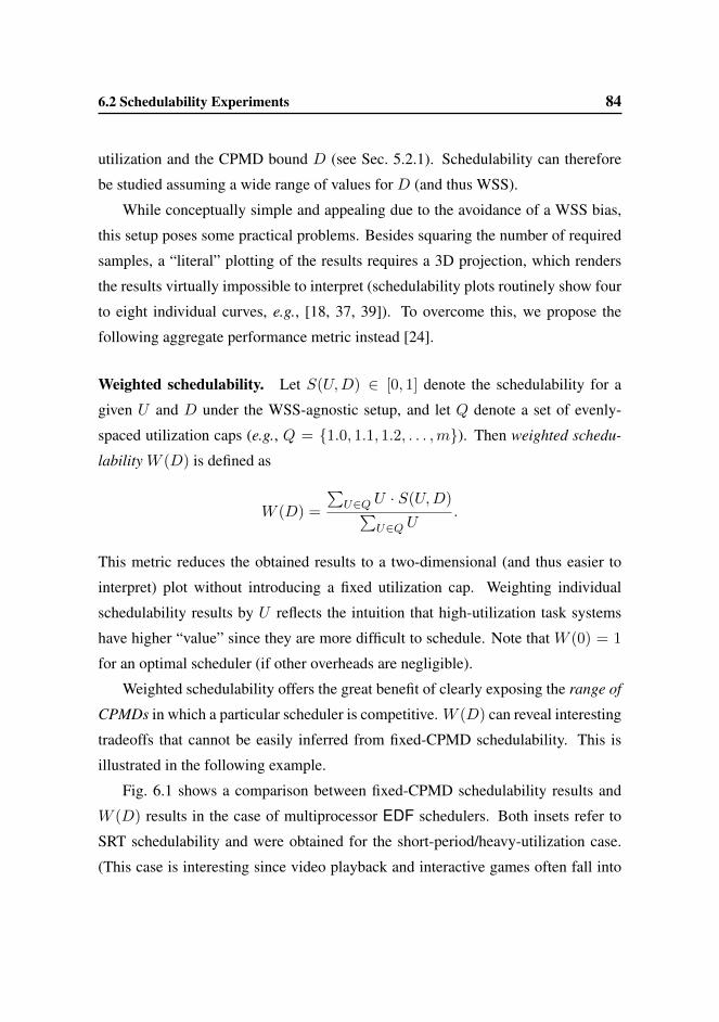
6.2 Schedulability Experiments 84
utilization and the CPMD bound D (see Sec. 5.2.1). Schedulability can therefore
be studied assuming a wide range of values for D (and thus WSS).
While conceptually simple and appealing due to the avoidance of a WSS bias,
this setup poses some practical problems. Besides squaring the number of required
samples, a “literal” plotting of the results requires a 3D projection, which renders
the results virtually impossible to interpret (schedulability plots routinely show four
to eight individual curves, e.g., [18, 37, 39]). To overcome this, we propose the
following aggregate performance metric instead [24].
Weighted schedulability. Let S(U,D) ∈ [0, 1] denote the schedulability for a
given U and D under the WSS-agnostic setup, and let Q denote a set of evenly-
spaced utilization caps (e.g., Q = {1.0, 1.1, 1.2, . . . ,m}). Then weighted schedu-
lability W (D) is defined as
W (D) =
∑U∈Q U · S(U,D)∑
U∈Q U.
This metric reduces the obtained results to a two-dimensional (and thus easier to
interpret) plot without introducing a fixed utilization cap. Weighting individual
schedulability results by U reflects the intuition that high-utilization task systems
have higher “value” since they are more difficult to schedule. Note that W (0) = 1
for an optimal scheduler (if other overheads are negligible).
Weighted schedulability offers the great benefit of clearly exposing the range of
CPMDs in which a particular scheduler is competitive. W (D) can reveal interesting
tradeoffs that cannot be easily inferred from fixed-CPMD schedulability. This is
illustrated in the following example.
Fig. 6.1 shows a comparison between fixed-CPMD schedulability results and
W (D) results in the case of multiprocessor EDF schedulers. Both insets refer to
SRT schedulability and were obtained for the short-period/heavy-utilization case.
(This case is interesting since video playback and interactive games often fall into

6.2 Schedulability Experiments 85
P-EDF C-EDF-L2 C-EDF-L3 G-EDF[1] [2] [3] [4]
0
0.2
0.4
0.6
0.8
1
0 5 10 15 20 25
ratio
of s
ched
ulab
le ta
sk s
ets
[sof
t]
task set utilization cap (prior to inflation)
CPMD = 500.00; utilization uniformly in [0.5, 0.9]; period uniformly in [3, 33]
[1] [2]
[3]
[4]
(a)
0
0.2
0.4
0.6
0.8
1
0 500 1000 1500 2000
wei
ghte
d sc
hedu
labi
lity
[sof
t]
cache-related preemption/migration delay (in us)
utilization uniformly in [0.5, 0.9]; period uniformly in [3, 33]
[3][4]
[2]
[1]
(b)
Figure 6.1: Comparison of fixed-CPMD and W (D) schedulability. The graphs show SRTschedulability for the uniform heavy utilization distribution with short periods. (a) Schedu-lability as function of U for CPMD = 500µs. (b) W (D) schedulability as function ofCPMD. Note the different x-axis in each inset.
6.3 Evaluation of Multiprocessor EDF Scheduling Algorithms 86
the period range [3ms, 33ms], and high-definition multimedia processing is likely
to cause heavy utilizations.) Fig. 6.1(a) indicates the fraction of generated task
sets each algorithm successfully scheduled, as a function of total utilization and
assuming a fixed D of 500µs. As can be observed in Fig. 5.6(a), this cache-related
delay is the average delay experienced by tasks with a WSS of 512 KB on our
platform for both preemptions and migrations when the system is under load. As
can be seen, C-EDF-L3 is the best performing algorithm. C-EDF-L2 and P-EDF
exhibit similar, but worse, performance. These trends arise if D = 500µs for both
preemption and migration costs, but if preemptions were considerably cheaper than
migrations, would P-EDF perform better than C-EDF-L3? Fig. 6.1 (a) does not
give any insight as to how to answer this question.
In contrast, the W (D) graph in Fig. 6.1 (b) provides an immediate answer. In-
set (a) collapses to four distinct points (one for each algorithm) at D = 500 in
inset (b). Inset (b) indicates weighted schedulability as a function of CPMD D. In
this plot, the curve for C-EDF-L3 reveals that for D ≤ 600µs, C-EDF-L3 is supe-
rior to P-EDF. Therefore, if the cost of migrations is less than 600µs, C-EDF-L3
should be preferred to P-EDF, even if the cost of preemptions is 0µs. We believe
that weighted schedulability plots are a valuable aid that may help practitioners to
select an appropriate real-time scheduler to use, basing the choice on actual mea-
sured CPMD values.
6.3 Evaluation of Multiprocessor EDF Scheduling Algorithms
The empirical comparison of P-EDF, G-EDF, and C-EDF proposed in this section
allows to answer questions on the implementation of clustered algorithms. In fact,
questions regarding the performance of such algorithms in comparison to global
and partitioned algorithms have not been fully answered by previous studies. Par-
ticularly, in [45], clustering is considered only in the context of SRT systems and
the presented evaluation is based on an architecture simulator. In [39], due to ar-
6.3 Evaluation of Multiprocessor EDF Scheduling Algorithms 87
chitectural limitations, only one cluster size could be considered. If multiple lev-
els of shared cache exist, it is not clear which level should be used for clustering.
Additionally, preemption/migration costs are assumed in [39] based on a fixed per-
job working set size. It is not clear whether similar conclusions would have been
reached for other cost choices.
Following the WSS-agnostic approach described above, in the comparison of
multiprocessor EDF schedulers we chose to varyD over [0µs, 2000µs]. This range
of values seems reasonable on a platform like ours, where (as noted in Sec. 5.2.2)
cache-related delays are non-predictable for WSSs that exceed the size of L2 cache
and the average-case delay for a 1024 KB WSS in a system under load is approxi-
mately 1000µs.
Schedulability was checked for different categories of task systems under P-
EDF, G-EDF, C-EDF-L2, and C-EDF-L3. For P-EDF and both variants of C-
EDF, we determined whether each task set could be partitioned using the worst-fit
decreasing heuristic. Under P-EDF, HRT and SRT schedulability differ only in the
use of maximum or average overheads: under partitioning, if tardiness is bounded,
then it is zero, so the only way to schedule a SRT task set is to view it as hard. Under
C-EDF, schedulability for each cluster was checked by applying the appropriate G-
EDF test (HRT or SRT) within the cluster.
HRT schedulability under G-EDF (C-EDF) was determined by testing whether
a given task set (cluster) passes at least one of five major sufficient — but not nec-
essary — HRT schedulability test [17, 20, 28, 29, 61]. For SRT schedulability,
since G-EDF can guarantee bounded deadline tardiness if the system is not over-
loaded [53], only a check that total utilization is at most m (the number of proces-
sors) is required.
Contrary to previous studies (e.g., [37, 39]), we further compared HRT schedu-
lability results with results obtained from “brute-force” (BF) schedulability tests. In
such a test, simulation (with overheads considered) is used to produce a periodic
schedule, and a task set is deemed to be unschedulable if any deadline misses are
6.3 Evaluation of Multiprocessor EDF Scheduling Algorithms 88
found. Given the very large hyperperiods of the generated task sets, exhaustive sim-
ulations were infeasible. Thus, each task set was simulated for 60 seconds or until a
deadline miss was found. Results from such BF tests represent an upper bound on
schedulability for each tested algorithm: task sets claimed unschedulable by a BF
test are certainly not schedulable, while a BF test may wrongly claim as schedulable
task sets that miss a deadline at a later point in the schedule, or that exhibit deadline
misses only under non-periodic arrival sequences. Note that, since EDF is optimal
on uniprocessors, a BF test is not of interest for P-EDF: if a task set can be suc-
cessfully partitioned onto individual processors, then no job will miss a deadline,
and simulating a schedule is therefore pointless. For each algorithm, and for each
(U,D) pair, we compared W (D) and BF (except for P-EDF) by testing 1,000 task
sets. Considering a spacing of 0.25 for U and a spacing of 100µs for D, more than
7.5 million task sets were evaluated.
Results. HRT W (D) results for the moderate period distributions are shown in
Fig. 6.2 and Fig. 6.3. Fig. 6.2 gives results for the three uniform distributions
(light, medium, heavy) and Fig. 6.3 gives results for the three bimodal distributions.
The plots indicate both W (D) and BF test results for D ranging over [0, 2000µs].
Weighted schedulability results for the SRT case are shown in Fig. 6.4 (uniform dis-
tributions) and Fig. 6.5 (bimodal distributions). All weighted schedulability graphs
are reported in Appendix B.2, while the complete set of all graphs (both weighted
and actual schedulability) can be found in the extended version of [23].
Observation 6.3.1. G-EDF is never preferable for HRT on our platform. In fact,
Fig. 6.2 and Fig. 6.3 show that theW (D) curve for P-EDF dominates the BF curves
of all the other algorithms in most graphs, independently of preemption/migration
costs. The BF test is optimistic and represents an upper bound on the schedulability
of G-EDF and C-EDF. Therefore, even if a perfect G-EDF feasibility test (i.e., a
test that never wrongly claims a schedulable task set as unschedulable) were em-
ployed, G-EDF would still not be preferable to P-EDF in most cases, even when

6.3 Evaluation of Multiprocessor EDF Scheduling Algorithms 89
P-EDF W(D) C-EDF-L2 W(D) C-EDF-L3 W(D) G-EDF W(D) C-EDF-L2 BF C-EDF-L3 BF G-EDF BF[1] [2] [3] [4] [5] [6] [7]
0
0.2
0.4
0.6
0.8
1
0 500 1000 1500 2000
wei
ghte
d sc
hedu
labi
lity
[har
d]
cache-related preemption/migration delay (in us)
utilization uniformly in [0.001, 0.1]; period uniformly in [10, 100]
[1]
[5]
[2][6]
[3] [7] [4]
(a)
0
0.2
0.4
0.6
0.8
1
0 500 1000 1500 2000
wei
ghte
d sc
hedu
labi
lity
[har
d]
cache-related preemption/migration delay (in us)
utilization uniformly in [0.1, 0.4]; period uniformly in [10, 100]
[4]
[3]
[7]
[2]
[1] [5] [6]
(b)
0
0.2
0.4
0.6
0.8
1
0 500 1000 1500 2000
wei
ghte
d sc
hedu
labi
lity
[har
d]
cache-related preemption/migration delay (in us)
utilization uniformly in [0.5, 0.9]; period uniformly in [10, 100]
[7]
[4][1,2,3,5,6]
(c)
Figure 6.2: HRT weighted schedulability for moderate periods as a function of cache-related preemption/migration cost for various utilization distributions. (a) Uniform light.(b) Uniform medium. (c) Uniform heavy. Recall that CPMD is the extra delay a job incursdue to a loss of cache affinity when resuming execution after a preemption or a migration.Note that these graphs allow meaningful comparisons between different x-coordinates —e.g., a particular workload may incur only 200µs CPMD under C-EDF and 400µs underG-EDF (see Sec. 6.2.2 for an in-depth explanation of weighted schedulability).

6.3 Evaluation of Multiprocessor EDF Scheduling Algorithms 90
P-EDF W(D) C-EDF-L2 W(D) C-EDF-L3 W(D) G-EDF W(D) C-EDF-L2 BF C-EDF-L3 BF G-EDF BF[1] [2] [3] [4] [5] [6] [7]
0
0.2
0.4
0.6
0.8
1
0 500 1000 1500 2000
wei
ghte
d sc
hedu
labi
lity
[har
d]
cache-related preemption/migration delay (in us)
util. bimodially in [0.001, 0.5] (8/9) and [0.5, 0.9] (1/9); period uniformly in [10, 100]
[1]
[5]
[6]
[3]
[4]
[7] [2]
(a)
0
0.2
0.4
0.6
0.8
1
0 500 1000 1500 2000
wei
ghte
d sc
hedu
labi
lity
[har
d]
cache-related preemption/migration delay (in us)
util. bimodially in [0.001, 0.5] (6/9) and [0.5, 0.9] (3/9); period uniformly in [10, 100]
[1]
[5]
[3]
[4]
[2]
[6] [7]
(b)
0
0.2
0.4
0.6
0.8
1
0 500 1000 1500 2000
wei
ghte
d sc
hedu
labi
lity
[har
d]
cache-related preemption/migration delay (in us)
util. bimodially in [0.001, 0.5] (4/9) and [0.5, 0.9] (5/9); period uniformly in [10, 100]
[1]
[4]
[2]
[3]
[7] [5] [6]
(c)
Figure 6.3: HRT weighted schedulability for moderate periods as a function of cache-related preemption/migration cost for various utilization distributions. (a) Bimodal light.(b) Bimodal medium. (c) Bimodal heavy. Recall that CPMD is the extra delay a job incursdue to a loss of cache affinity when resuming execution after a preemption or a migra-tion. As noted in Fig. 6.2, these graphs allow meaningful comparisons between differentx-coordinates.
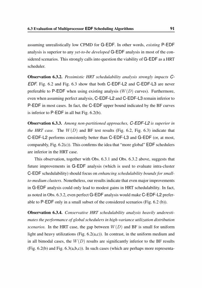
6.3 Evaluation of Multiprocessor EDF Scheduling Algorithms 91
assuming unrealistically low CPMD for G-EDF. In other words, existing P-EDF
analysis is superior to any yet-to-be developed G-EDF analysis in most of the con-
sidered scenarios. This strongly calls into question the viability of G-EDF as a HRT
scheduler.
Observation 6.3.2. Pessimistic HRT schedulability analysis strongly impacts C-
EDF. Fig. 6.2 and Fig. 6.3 show that both C-EDF-L2 and C-EDF-L3 are never
preferable to P-EDF when using existing analysis (W (D) curves). Furthermore,
even when assuming perfect analysis, C-EDF-L2 and C-EDF-L3 remain inferior to
P-EDF in most cases. In fact, the C-EDF upper bound indicated by the BF curves
is inferior to P-EDF in all but Fig. 6.2(b).
Observation 6.3.3. Among non-partitioned approaches, C-EDF-L2 is superior in
the HRT case. The W (D) and BF test results (Fig. 6.2, Fig. 6.3) indicate that
C-EDF-L2 performs consistently better than C-EDF-L3 and G-EDF (or, at most,
comparably, Fig. 6.2(c)). This confirms the idea that “more global” EDF schedulers
are inferior in the HRT case.
This observation, together with Obs. 6.3.1 and Obs. 6.3.2 above, suggests that
future improvements in G-EDF analysis (which is used to evaluate intra-cluster
C-EDF schedulability) should focus on enhancing schedulability bounds for small-
to-medium clusters. Nonetheless, our results indicate that even major improvements
in G-EDF analysis could only lead to modest gains in HRT schedulability. In fact,
as noted in Obs. 6.3.2, even perfect G-EDF analysis would make C-EDF-L2 prefer-
able to P-EDF only in a small subset of the considered scenarios (Fig. 6.2 (b)).
Observation 6.3.4. Conservative HRT schedulability analysis heavily underesti-
mates the performance of global schedulers in high-variance utilization distribution
scenarios. In the HRT case, the gap between W (D) and BF is small for uniform
light and heavy utilizations (Fig. 6.2(a,c)). In contrast, in the uniform medium and
in all bimodal cases, the W (D) results are significantly inferior to the BF results
(Fig. 6.2(b) and Fig. 6.3(a,b,c)). In such cases (which are perhaps more representa-

6.3 Evaluation of Multiprocessor EDF Scheduling Algorithms 92
tive of real-world workloads), task utilizations may vary greatly. Existing G-EDF
analysis is unable to fully characterize such variations and therefore the W (D) re-
sults for G-EDF and C-EDF are noticeably lower than the BF results. Instead,
when utilization is uniformly light, all task sets are comprised of many small tasks,
which are significantly affected by overheads. In this context, all algorithms per-
form poorly, and conservative schedulability bounds are quite close (Fig. 6.2(a)). In
the uniform heavy utilization case, overheads have a minor impact on the few large
tasks that compose each task set. Nonetheless, given their utilizations, such task
sets are difficult to schedule and W (D) correctly approximates BF (Fig. 6.2(c)).
Observation 6.3.5. Bin-packing limitations are mostly negligible for clusters of size
six. If the system is not overutilized, G-EDF is optimal for SRT (i.e., G-EDF guar-
antees bounded tardiness for any task set with total utilization at mostm); therefore,
if a task set can be partitioned under C-EDF, then it is schedulable for SRT. Since
the schedulability test for SRT is not pessimistic, Fig. 6.4 and Fig. 6.5 (which report
SRT W (D) results) reveals a tradeoff between bin-packing and overheads. When
bin-packing limitations are not an issue (because all task utilizations are small —
Fig. 6.4(a)), lower overheads favor P-EDF and C-EDF-L2 over C-EDF-L3 and
G-EDF. Instead, bin-packing limitations clearly affect P-EDF when task utiliza-
tions are heavy: Fig. 6.4(c) and Fig. 6.5(c) shows that a small increase in cluster
size (from one core — P-EDF— to two cores — C-EDF-L2) is sufficient to boost
performance. In particular, Fig. 6.4 and Fig. 6.5 show that bin-packing is not a lim-
itation for C-EDF-L3: W (D) curves for C-EDF-L3 are as high as G-EDF curves
in all insets. Since bin-packing problems become easier with larger and fewer bins,
clusters of size six (or larger) are sufficient to avoid bin-packing limitations in the
majority of the tested scenarios. Previous studies based on an architecture simula-
tor [45] have shown that a cluster size of four may be sufficient to avoid bin-packing
issues, but, due to the topology of our platform, such cluster size is not desirable.
Given such results, we believe that future work on improving SRT tardiness bounds
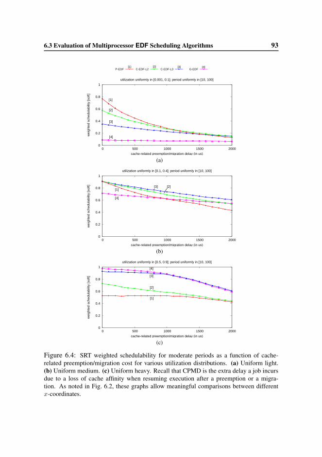
6.3 Evaluation of Multiprocessor EDF Scheduling Algorithms 93
P-EDF C-EDF-L2 C-EDF-L3 G-EDF[1] [2] [3] [4]
0
0.2
0.4
0.6
0.8
1
0 500 1000 1500 2000
wei
ghte
d sc
hedu
labi
lity
[sof
t]
cache-related preemption/migration delay (in us)
utilization uniformly in [0.001, 0.1]; period uniformly in [10, 100]
[1]
[2]
[3]
[4]
(a)
0
0.2
0.4
0.6
0.8
1
0 500 1000 1500 2000
wei
ghte
d sc
hedu
labi
lity
[sof
t]
cache-related preemption/migration delay (in us)
utilization uniformly in [0.1, 0.4]; period uniformly in [10, 100]
[1]
[4]
[3] [2]
(b)
0
0.2
0.4
0.6
0.8
1
0 500 1000 1500 2000
wei
ghte
d sc
hedu
labi
lity
[sof
t]
cache-related preemption/migration delay (in us)
utilization uniformly in [0.5, 0.9]; period uniformly in [10, 100]
[4]
[3]
[2]
[1]
(c)
Figure 6.4: SRT weighted schedulability for moderate periods as a function of cache-related preemption/migration cost for various utilization distributions. (a) Uniform light.(b) Uniform medium. (c) Uniform heavy. Recall that CPMD is the extra delay a job incursdue to a loss of cache affinity when resuming execution after a preemption or a migra-tion. As noted in Fig. 6.2, these graphs allow meaningful comparisons between differentx-coordinates.

6.3 Evaluation of Multiprocessor EDF Scheduling Algorithms 94
P-EDF C-EDF-L2 C-EDF-L3 G-EDF[1] [2] [3] [4]
0
0.2
0.4
0.6
0.8
1
0 500 1000 1500 2000
wei
ghte
d sc
hedu
labi
lity
[sof
t]
cache-related preemption/migration delay (in us)
util. bimodially in [0.001, 0.5] (8/9) and [0.5, 0.9] (1/9); period uniformly in [10, 100]
[3] [2]
[4]
[1]
(a)
0
0.2
0.4
0.6
0.8
1
0 500 1000 1500 2000
wei
ghte
d sc
hedu
labi
lity
[sof
t]
cache-related preemption/migration delay (in us)
util. bimodially in [0.001, 0.5] (6/9) and [0.5, 0.9] (3/9); period uniformly in [10, 100]
[3] [2]
[1]
[4]
(b)
0
0.2
0.4
0.6
0.8
1
0 500 1000 1500 2000
wei
ghte
d sc
hedu
labi
lity
[sof
t]
cache-related preemption/migration delay (in us)
util. bimodially in [0.001, 0.5] (4/9) and [0.5, 0.9] (5/9); period uniformly in [10, 100]
[3]
[1]
[2]
[4]
(c)
Figure 6.5: SRT weighted schedulability for moderate periods as a function of cache-related preemption/migration cost for various utilization distributions. (a) Bimodal light.(b) Bimodal medium. (c) Bimodal heavy. Recall that CPMD is the extra delay a job incursdue to a loss of cache affinity when resuming execution after a preemption or a migra-tion. As noted in Fig. 6.2, these graphs allow meaningful comparisons between differentx-coordinates.
6.4 Evaluation of Semi-Partitioned Algorithms 95
should focus on platforms with at most four to eight cores.
Observation 6.3.6. The C-EDF approaches are superior to the other algorithms
in the SRT case. In the majority of the tested scenarios (Fig. 6.4 and Fig. 6.5), C-
EDF-L3 and C-EDF-L2 usually performed better than G-EDF and P-EDF even
under moderate-to-high migration costs and low preemption costs. For example, in
Fig. 6.5(a), the C-EDF-L3 and C-EDF-L2 curves are as high as the P-EDF curve
even assuming 200µs for migrations and 0µs for preemptions! C-EDF-L3 gen-
erally exhibits slightly higher schedulability than C-EDF-L2, while both C-EDF
approaches have lower overheads than G-EDF.
6.4 Evaluation of Semi-Partitioned Algorithms
In this section, we present the results of the empirical comparison of EDF-fm, EDF-
WM, NPS-F, and C-NPS-F. Particularly, in Sec. 6.4.1 and Sec. 6.4.2 we discuss
the results of our experiments, while in Sec. 6.4.3 we summarize several design
principles to aid the future development of practical semi-partitioned algorithms.
As shown in Sec. 6.3 and in previous studies [25, 37, 39], P-EDF (resp. C-EDF) is
particularly effective for HRT (resp. SRT) workloads. Therefore, in the evaluations
presented in this section, we use P-EDF and C-EDF as a basis of comparison.
In the evaluation of multiprocessor EDF schedulers described above (Sec. 6.3),
a single (worst-case) CPMD value was assumed for both preemptions and the var-
ious kinds of migrations that can occur (through L2, L3, and main memory, re-
spectively) when assessing the schedulability of a task set. Such an approach is
problematic for our purposes here, as semi-partitioned algorithms are designed to
lessen the impact of migrations. Thus, in the comparison of semi-partitioned algo-
rithms, we express the different D values measured on our platform as a function
of WSS. For example, considering WSS = 64 KB in an idle system, Fig. 5.5(b) tells
us that a preemption has a delay D = 1µs, a migration through an L2 cache has
D = 17µs, and L3 and memory migrations have D = 60µs. With such a mapping,
6.4 Evaluation of Semi-Partitioned Algorithms 96
the weighted-schedulability metric presented above (Sec. 6.2.2) becomes a function
of the assumed utilization cap U and the assumed WSS ξ.
W (ξ) =
∑U∈Q U · S(U, ξ)∑
U∈Q U.
In essence, one can think of ξ as a parameter that is used to determine an appro-
priate CPMD value D by indexing into either the graph in Fig. 5.5 or its average-
case-delay counterpart (Fig. 5.6).
Employing such modified weighted-schedulability performance metric, for each
algorithm and each pair (U, ξ), we determined W (ξ) by checking 100 task sets. We
varied U from one to 24 in steps of 0.25, and ξ over [0, 3072] KB in steps of 16 KB
for ξ ≤ 256 KB, in steps of 64 KB for 256 KB < ξ ≤ 1024 KB, and in steps of
256 KB for higher values. This allows for a higher resolution in the range of WSSs
that have low CPMD (D ≤ 1ms in a system under load — e.g., Fig. 5.5(a)). The
upper bound of 3072 KB for ξ was selected because measurements taken on our
test platform revealed (Fig. 5.6(a)) that CPMD becomes unpredictable (over many
measurements, standard deviations are large — see Sec. 5.2.2) for WSSs exceeding
this bound. We used maximum (resp., average) overhead and CPMD values to
determine weighted schedulability in the HRT (resp., SRT) case. For CPMD, both
loaded and idle systems were considered.
The schedulability of a single task set was checked as follows. For P-EDF and
C-EDF, we determined whether each task could be partitioned using the worst-fit
decreasing heuristic. For P-EDF (C-EDF), HRT (SRT) schedulability on each pro-
cessor (within each cluster) merely requires that that processor (cluster) is not over-
utilized. For EDF-fm, EDF-WM, NPS-F, and C-NPS-F, we determined schedu-
lability by using tests (SRT for EDF-fm, HRT for the others) presented by the de-
velopers of those algorithms; these tests were augmented to account for overheads,
as discussed earlier.
The considered scenarios resulted in 54 graphs of weighted schedulability data

6.4 Evaluation of Semi-Partitioned Algorithms 97
arising from testing the schedulability of approximately 7 million task systems un-
der each algorithm; when expanded to produce actual (not weighted) schedulability
plots, over 1,500 graphs are required. We only discuss a few representative weighted
schedulability graphs here. We further restrict our attention to ξ ≤ 1024 KB be-
cause all major trends manifest in this range. All weighted schedulability graphs
(for ξ ≤ 1024 KB) are reported in Appendix C.2, while the complete set of all
graphs (both weighted and actual schedulability, and for the full WSS range) can be
found in the extended version of [26].
6.4.1 NPS-F, C-NPS-F, and Choosing δ
NPS-F and C-NPS-F actually represent a “family” of different design choices, as
the behavior of each algorithm depends on the parameter δ. We begin with two
observations concerning these algorithms that allow us to reasonably constrain the
considered design choices for these algorithms in later graphs.
Observation 6.4.1. δ = 1 leads to higher schedulability than δ = 4. Under
NPS-F (Sec. 4.3), increasing δ leads to a higher utilization bound at the cost of
increased preemption frequency. In [33], Bletsas and Andersson presented a com-
parison of NPS-F’s schedulable utilization bounds with δ ranging over [1, 4]. δ = 4
was shown to yield a higher bound than δ = 1, at the cost of increased preemptions.
In contrast to this, we found that when overheads are considered, NPS-F schedula-
bility is almost always better with δ = 1 than with δ = 4 in both loaded and idle
systems. The difference can be observed in Fig. 6.6, which plots W (ξ) for NPS-F
for both idle systems and systems under load, for both δ = 1 and δ = 4. Fig. 6.6(a)
gives HRT schedulability results for medium exponential utilizations and moderate
periods, while Fig. 6.6(b) presents HRT schedulability results for light uniform uti-
lizations and long periods. In both insets, NPS-F schedulability is always better
with δ = 1 than with δ = 4. Accounting for overheads (particularly CPMD, the re-
duction of effective capacity available to tasks mentioned in Sec. 6.1, and overhead-
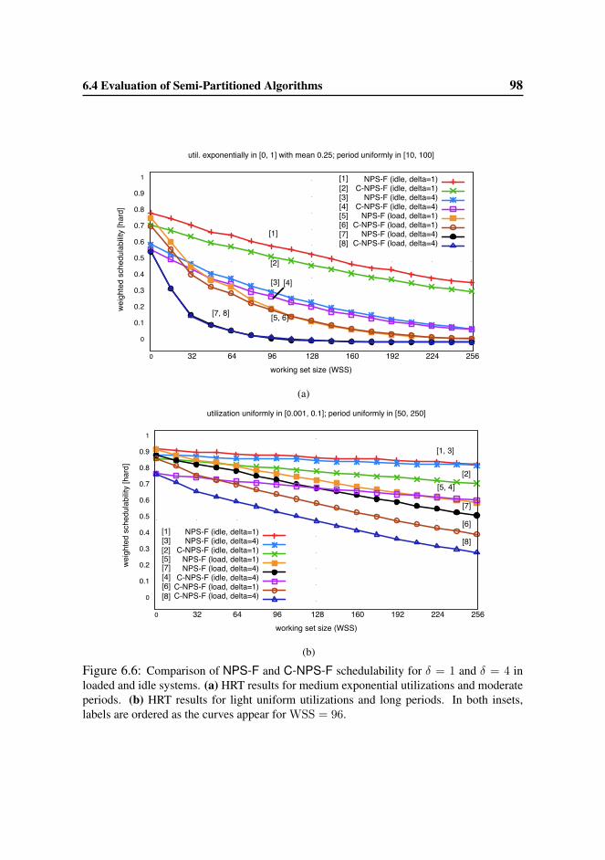
6.4 Evaluation of Semi-Partitioned Algorithms 98
0
0.1
0.2
0.3
0.4
0.5
0.6
0.7
0.8
0.9
1
0 32 64 96 128 160 192 224 256
weig
hted
sch
edul
abilit
y [h
ard]
working set size (WSS)
util. exponentially in [0, 1] with mean 0.25; period uniformly in [10, 100]
NPS-F (idle, delta=1)C-NPS-F (idle, delta=1)
NPS-F (idle, delta=4)C-NPS-F (idle, delta=4)
NPS-F (load, delta=1)C-NPS-F (load, delta=1)
NPS-F (load, delta=4)C-NPS-F (load, delta=4)
[1][2][3][4][5][6][7][8]
[1]
[2]
[3] [4]
[5, 6][7, 8]
(a)
0
0.1
0.2
0.3
0.4
0.5
0.6
0.7
0.8
0.9
1
0 32 64 96 128 160 192 224 256
weig
hted
sch
edul
abilit
y [h
ard]
working set size (WSS)
utilization uniformly in [0.001, 0.1]; period uniformly in [50, 250]
NPS-F (idle, delta=1)NPS-F (idle, delta=4)
C-NPS-F (idle, delta=1)NPS-F (load, delta=1)NPS-F (load, delta=4)
C-NPS-F (idle, delta=4)C-NPS-F (load, delta=1)C-NPS-F (load, delta=4)
[1]
[2][3]
[4]
[5]
[6]
[7]
[8]
[1, 3]
[2][5, 4]
[7]
[6]
[8]
(b)
Figure 6.6: Comparison of NPS-F and C-NPS-F schedulability for δ = 1 and δ = 4 inloaded and idle systems. (a) HRT results for medium exponential utilizations and moderateperiods. (b) HRT results for light uniform utilizations and long periods. In both insets,labels are ordered as the curves appear for WSS = 96.

6.4 Evaluation of Semi-Partitioned Algorithms 99
related bin-packing issues) in NPS-F analysis amplifies the effects of additional
overheads due to the increase in the number of preemptions and migrations (from
δ = 1 to δ = 4). In all the evaluated scenarios, we found δ = 4 to be competitive
with δ = 1 only when bin-packing issues and CPMD are negligible (for uniform
light distributions, and an idle system — e.g., Fig. 6.6(b)). Given Obs. 6.4.1, we
only consider the choice of δ = 1 in the graphs that follow.
Observation 6.4.2. C-NPS-F is almost never preferable to NPS-F. Fig. 6.6 (both
insets) shows that C-NPS-F is never preferable to NPS-F in idle systems or in
systems under load when δ = 1. Eliminating off-chip migrations in C-NPS-F ex-
acerbates bin-packing-related issues that arise when assigning servers to processors
and heavily constrains C-NPS-F schedulability. Because of its poor performance
in comparison to NPS-F, we do not consider C-NPS-F in the graphs that follow.
We note that Appendix C.2 and in the extended version of [26], C-NPS-F and
the choice of δ = 4 are considered in all graphs.
6.4.2 HRT and SRT Schedulability Results
Fig. 6.7 and Fig. 6.8 gives a subset of the weighted schedulability results obtained in
the comparison of semi-partitioned scheduling policies. Fig. 6.7 gives HRT schedu-
lability results for the exponential medium (inset (a)) and bimodal heavy (inset (b))
distributions, while Fig. 6.8 reports SRT results for the exponential medium (in-
sets (a)) and uniform heavy (inset (b)) distributions. The following observations are
supported by the data we collected in the context of this study.
Observation 6.4.3. EDF-WM is the best performing algorithm in the HRT case.
In the HRT case, EDF-WM overcomes bin-packing-related limitations that impact
P-EDF when many high-utilization tasks exist (Fig. 6.7(b)). More generally, EDF-
WM always exhibits schedulability in this case that is superior, or at worst compa-
rable (e.g., Fig. 6.7(a)), to that of P-EDF.

6.4 Evaluation of Semi-Partitioned Algorithms 100
P-EDF (load)P-EDF (idle)
EDF-WM (load)
EDF-WM (idle)NPS-F (idle, delta=1)
NPS-F (load, delta=1)
[1][2][3]
[4][5][6]
0
0.1
0.2
0.3
0.4
0.5
0.6
0.7
0.8
0.9
1
0 64 128 192 256 320 384 448 512 576 640 704 768 832 896 960 1024
weig
hted
sch
edul
abilit
y [h
ard]
working set size (WSS)
util. exponentially in [0, 1] with mean 0.25; period uniformly in [10, 100]
[1, 3]
[2, 4]
[5]
[6]
(a)
0
0.1
0.2
0.3
0.4
0.5
0.6
0.7
0.8
0.9
1
0 64 128 192 256 320 384 448 512 576 640 704 768 832 896 960 1024
weig
hted
sch
edul
abilit
y [h
ard]
working set size (WSS)
util. bimodally in [0.001, 0.5] (4/9) and [0.5, 0.9] (5/9); period uniformly in [10, 100]
[1]
[2]
[3][4]
[5][6]
(b)
Figure 6.7: Weighted schedulability as a function of WSS. (a) HRT results for medium ex-ponential utilizations and moderate periods. (b) HRT results for heavy bimodal utilizationsand moderate periods.
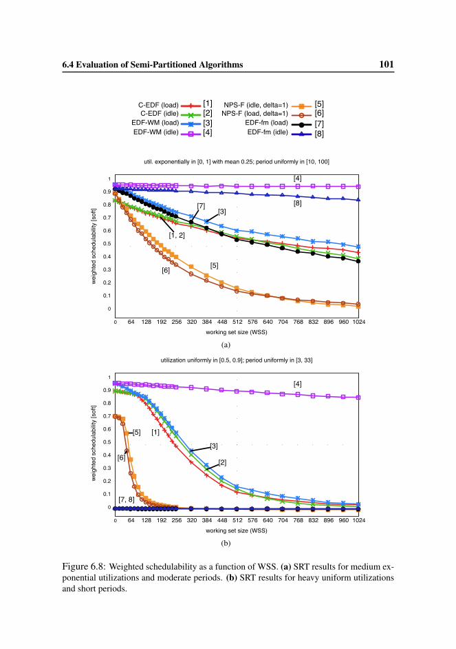
6.4 Evaluation of Semi-Partitioned Algorithms 101
C-EDF (load)C-EDF (idle)
EDF-WM (load)EDF-WM (idle)
NPS-F (idle, delta=1)NPS-F (load, delta=1)
EDF-fm (load)EDF-fm (idle)
[1][2][3][4]
[5][6][7][8]
0
0.1
0.2
0.3
0.4
0.5
0.6
0.7
0.8
0.9
1
0 64 128 192 256 320 384 448 512 576 640 704 768 832 896 960 1024
weig
hted
sch
edul
abilit
y [s
oft]
working set size (WSS)
util. exponentially in [0, 1] with mean 0.25; period uniformly in [10, 100]
[1, 2]
[3]
[4]
[5][6]
[7] [8]
(a)
0
0.1
0.2
0.3
0.4
0.5
0.6
0.7
0.8
0.9
1
0 64 128 192 256 320 384 448 512 576 640 704 768 832 896 960 1024
weig
hted
sch
edul
abilit
y [s
oft]
working set size (WSS)
utilization uniformly in [0.5, 0.9]; period uniformly in [3, 33]
[1]
[2]
[3]
[4]
[5]
[6]
[7, 8]
(b)
Figure 6.8: Weighted schedulability as a function of WSS. (a) SRT results for medium ex-ponential utilizations and moderate periods. (b) SRT results for heavy uniform utilizationsand short periods.

6.4 Evaluation of Semi-Partitioned Algorithms 102
Observation 6.4.4. EDF-WM outperforms C-EDF in the SRT case. Fig. 6.8(a)
shows that, for C-EDF, schedulability decreases quickly as WSS increases due to
bin-packing limitations, which are exacerbated by high(er) overheads due to higher
run-queue contention. In contrast, EDF-WM exhibits good schedulability over the
whole range of tested WSSs when preemption costs are cheaper than migration costs
(see the idle curves in Fig. 6.8(a,b)). This is mainly due to the reduced number of
migrations and their pre-planned nature under EDF-WM. Furthermore, even when
cache-related migration costs are not substantially worse than preemption costs (see
the load curves in Fig. 6.8(a,b)), EDF-WM is effective in overcoming bin-packing
issues and, due to reduced run-queue contention, it achieves higher schedulability
than C-EDF.
Observation 6.4.5. EDF-fm usually performs better than C-EDF in the SRT case.
Like EDF-WM, when preemption costs are less than migration costs and when
most tasks have low utilization (e.g., the idle curves in Fig. 6.8(a)), EDF-fm is
effective in overcoming bin-packing limitations and achieves higher schedulability
than C-EDF. However, due to the utilization constraint EDF-fm imposes on migra-
tory tasks, it is unable to schedule task sets where most tasks have high utilization
(Fig. 6.8(b)). In addition, compared to EDF-WM, the higher number of migrations
affects EDF-fm schedulability when the costs of migrations are not substantially
worse than those of preemptions. For example, in Fig. 6.8(a), EDF-fm achieves
higher schedulability under load than C-EDF only when ξ ≤ 448 KB.
Observation 6.4.6. NPS-F is inferior to the other scheduling approaches in most
of the analyzed scenarios. In Fig. 6.7 and Fig. 6.8, schedulability under NPS-F is
lower than that of all the other evaluated scheduling policies in all depicted scenar-
ios (HRT and SRT). NPS-F schedulability is heavily constrained by the pessimistic
assumptions made in the bin-packing heuristics of NPS-F’s assignment phase, and
by higher preemption and migration delays. NPS-F achieves better schedulability
results than the other algorithms only when bin-packing issues are negligible and
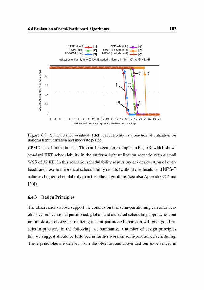
6.4 Evaluation of Semi-Partitioned Algorithms 103
0
0.2
0.4
0.6
0.8
1
1 2 3 4 5 6 7 8 9 10 11 12 13 14 15 16 17 18 19 20 21 22 23 24
ratio
of s
ched
ulab
le ta
sk s
ets
[har
d]
task set utilization cap (prior to overhead accounting)
utilization uniformly in [0.001, 0.1]; period uniformly in [10, 100]; WSS = 32kB
P-EDF (load)P-EDF (idle)
EDF-WM (load)
EDF-WM (idle)NPS-F (idle, delta=1)
NPS-F (load, delta=1)
P-EDF (load)P-EDF (idle)
EDF-WM (load)
EDF-WM (idle)NPS-F (idle, delta=1)
NPS-F (load, delta=1)
[1][2][3]
[4][5][6]
[1] [2]
[3]
[5]
[4]
[6]
Figure 6.9: Standard (not weighted) HRT schedulability as a function of utilization foruniform light utilization and moderate period.
CPMD has a limited impact. This can be seen, for example, in Fig. 6.9, which shows
standard HRT schedulability in the uniform light utilization scenario with a small
WSS of 32 KB. In this scenario, schedulability results under consideration of over-
heads are close to theoretical schedulability results (without overheads) and NPS-F
achieves higher schedulability than the other algorithms (see also Appendix C.2 and
[26]).
6.4.3 Design Principles
The observations above support the conclusion that semi-partitioning can offer ben-
efits over conventional partitioned, global, and clustered scheduling approaches, but
not all design choices in realizing a semi-partitioned approach will give good re-
sults in practice. In the following, we summarize a number of design principles
that we suggest should be followed in further work on semi-partitioned scheduling.
These principles are derived from the observations above and our experiences in
6.4 Evaluation of Semi-Partitioned Algorithms 104
implementing the various semi-partitioned algorithms considered in this thesis.
Avoid unneeded migrations. EDF-WM reduces to pure partitioning when task
utilizations are low (no task needs to migrate). In contrast, EDF-fm and NPS-F
migrate tasks even in low-utilization contexts where partitioning would have been
sufficient. This increases overheads and contributes to their lower schedulability
(Obs. 6.4.5 and 6.4.6).
Minimize the number of preemptions. Avoiding migrations by increasing pre-
emption frequency can negatively impact schedulability. This was one of the issues
considered in Obs. 6.4.1, where increased preemption frequency was seen to lower
schedulability under NPS-F. Also, in many cases, the difference in the cost of a
preemption and that of a migration through L2, L3, or memory is not significant
(particularly, in a system under load, as seen in Fig. 5.5(a), and Fig. 5.6(a)). Thus,
favoring preemptions over migrations generally, L2 over L3 migrations, etc., may
not lead to improved schedulability (Obs. 6.4.2).
Minimize the number of tasks that may migrate. Migrating servers with tens of
tasks—any of which could incur CPMD—increases analysis pessimism and leads
to lower schedulability (Obs. 6.4.6). Higher schedulability is achieved by bounding
the number of migrating tasks (Obs. 6.4.3, and 6.4.4).
Avoid pull-migrations in favor of push-migrations. Push-migrations entail lower
overheads than pull-migrations (Sec. 5.1.2). This is because push-migrations can
be planned for in advance, while pull-migrations occur in a reactive way. Due to
this difference, push-migrations require only mostly-local state within per-CPU run
queues, while pull-migrations require global state and shared run queues. High
overhead due to run-queue contention is one reason why schedulability is generally
lower under C-EDF than under EDF-WM and EDF-fm (Obs. Obs. 6.4.4 and 6.4.5).
One of the key virtues of (most) semi-partitioned algorithms is that they enact mi-
grations by following a pre-planned strategy; this is unlike how migrations occur
under most conventional global and clustered algorithms.
Migration rules should be process-stack-aware. Migrations and context switch-
6.4 Evaluation of Semi-Partitioned Algorithms 105
es are not “instantaneous”; situations where migrating tasks are immediately eligi-
ble on another CPU (e.g., at an NPS-F slot boundary) need careful process-stack
management (so that each task executes on a single CPU only) that is tricky to im-
plement and entails analysis pessimism. In fact, analytically, proper accounting for
such hand-offs involves self-suspending the destination processor until the source
processor switches out the migrating task.
Use simple migration logic. Migrating tasks at job boundaries (task migration)
is preferable to migrating during job execution (job migration). Migrations of the
former type entail less overhead, are easier to implement, and are more predictable.
This results in a much simpler admission test (e.g., EDF-fm’s), particularly when
overheads must be considered.
Be cognizant of overheads when designing task assignment heuristics. Such
heuristics are crucial for an algorithm’s performance and should have an overhead-
aware design to avoid excessive pessimism (Obs. 6.4.2 and 6.4.6).
Avoid two-step task assignments. With double bin-packing, pessimistic analy-
sis assumptions concerning the second phase must be applied when analyzing the
first phase. For example, when analyzing the first assignment phase of NPS-F,
pessimistic accounting is needed for migrating servers, because the second phase
determines which servers actually migrate.
Chapter 7
Conclusions
The widespread diffusion of multicore platforms as computing platforms for embed-
ded, ruggedized systems (traditionally based on uniprocessor single-board comput-
ers) necessitates the deployment of practical implementations of real-time schedul-
ing algorithms that specifically target multiprocessor and multicore platforms. Such
algorithms should overcome the drawbacks of porting uniprocessor real-time sched-
uling to multiprocessor and multicore platforms. Unfortunately, in recent work on
multicore real-time scheduling algorithms, implementation-oriented issues and the
impact of OS and cache-related overheads have not received much attention.
Particularly, prior work on evaluating the impact of overheads on multiprocessor
real-time scheduling algorithms did not define methodologies to evaluate cache-
related preemption and migration delays on complex multicore platforms and did
not fully tackle the viability of clustered EDF algorithms in hard and soft real-time
contexts. Furthermore, no prior work exists that investigates the practical viability
of recent, yet promising, semi-partitioned scheduling techniques. In Ch. 5 and 6,
we addressed such shortcomings by presenting empirical methodologies to measure
cache-related overheads and by investigating the practical viability of clustered EDF
and semi-partitioned scheduling algorithms. In addition, to avoid biases towards
specific working set sizes (and therefore towards specific cache-related delays), we
proposed a new performance metric that enables the evaluation of an algorithm’s
106

7.1 Summary of Results 107
schedulability for wide ranges of cache-related preemption and migration delays.
7.1 Summary of Results
Motivated by the abovementioned observations, the proposed goal of this thesis
was to complement theoretical research on multiprocessor real-time scheduling by
evaluating the impact of implementation strategies and overheads on multiprocessor
and multicore real-time scheduling algorithms.
To support the above goal, in Ch. 5, we presented two empirical methods (sched-
ule-sensitive and synthetic) to measure cache-related preemption and migration de-
lays on platforms with a complex cache layout. Our findings show that, on our
24-core platform, CPMD in a system under load is only predictable for WSSs that
do not thrash the L2 cache. Furthermore, we observed that preemption and mi-
gration delays did not differ significantly in a system under load. This calls into
question the widespread belief that migrations always cause more delays than pre-
emptions. In particular, our data indicates that (on our platform) preemptions and
migrations differ only little in terms of both worst-case and average-case CPMD if
cache affinity is lost completely in the presence of either a background workload
or other real-time tasks with large WSSs. Also, our experiments showed that the
incurred CPMD depends on preemption length, but not on task set size.
To evaluate how implementation strategies and overheads impact the perfor-
mance (expressed in terms of algorithms’ schedulability) of multicore scheduling
algorithms, the effects of OS overheads and cache-related overheads (as measured
in Ch. 5) have been explicitly accounted for in the evaluations presented in Sec. 6.3
and 6.4. Furthermore, in those sections we have employed a new weighted schedu-
lability performance metric (Sec. 6.2.2) that allows to give guidelines on ranges of
CPMDs where a particular scheduling algorithm is competitive.
On our platform, the comparison of P-EDF, G-EDF, and C-EDF (Sec. 6.3)
under consideration of real overheads, indicates that G-EDF is never preferable for

7.1 Summary of Results 108
HRT. In most of the considered scenarios, existing P-EDF analysis was superior
not only to existing G-EDF analysis, but also to optimistic upper bounds for any
yet-to-be-developed G-EDF analysis. Furthermore, if the cost of migrations is non-
negligible, then the high schedulability gap between P-EDF and the other tested
algorithms calls into question the benefits of migrations for EDF scheduling algo-
rithms in the HRT case on large multicore platforms. In the HRT case, C-EDF-L2
(that clusters around the L2 cache) performed best among the non-partitioned algo-
rithms, although the pessimism of G-EDF analysis (particularly for workloads with
high-variance utilization distribution) strongly impacted C-EDF. Our results also
show that, practically speaking, bin-packing limitations are negligible for clusters
of size six. Therefore, our findings suggest that future HRT global scheduling re-
search should focus on small/medium-sized platforms. In the SRT case, the C-EDF
approaches (C-EDF-L3— that clusters around the L3 cache — in particular) were
superior to all other evaluated algorithms. Thus, future work on tardiness bounds
under G-EDF should focus on low processor counts (four to eight), as they are en-
countered under C-EDF during intra-cluster analysis. To the best of our knowledge,
our evaluation of multiprocessor EDF scheduling algorithms is the first to present a
comparison of C-EDF real-time schedulability for multiple cluster sizes assuming
real hardware overheads.
To understand the practical viability of recently-proposed semi-partitioned ap-
proaches, in Sec. 6.4, we presented the first empirical study of semi-partitioned mul-
tiprocessor real-time scheduling algorithms under consideration of real-world over-
heads. Our results indicate that, from a schedulability perspective, semi-partitioned
scheduling is often better than other alternatives. Most importantly, semi-partitioned
schedulers can benefit from the pre-planned nature of push-migrations: because it
is known ahead of time which task will migrate, and also among which proces-
sors, CPMD accounting is task-specific and hence less pessimistic. Furthermore,
since push-migrations can be implemented with mostly-local state, kernel overheads
are much lower in schedulers that avoid pull-migrations. These advantages can be

7.2 Future Work 109
clearly observed in those scenarios that are the main target of semi-partitioned al-
gorithms (i.e., scenarios in which the cost of preemptions is lower than the cost of
migrations). In addition, our results show that bounding the number of migrating
tasks improves the schedulability of semi-partitioned algorithms in those scenarios
in which migration costs are not substantially greater than preemption costs.
7.2 Future Work
There are several directions for future work and for extending the results presented
in this thesis, as we detail next.
Cache-related preemption and migration delays. Our evaluation used the TSC
to indirectly measure CPMD. It would be interesting to substitute the TSC with per-
formance counters to directly measure cache misses. Furthermore, since our plat-
form is a rather large UMA platform, it would be interesting to apply our methodolo-
gies to platforms that employ different cache layouts and different cache-coherence
protocols (e.g., embedded systems or NUMA platforms). Also, additional details
on cache-related overheads could be obtained by repeating our experiments in the
presence of heavy-load on the bus (e.g., frequent DMA - I/O transfers, etc.), or when
the bus is frequently locked by atomic operations.
Multiprocessor EDF algorithms. Several interesting questions exists pertaining
to the clustered EDF policy. Particularly, it would be interesting to investigate the
behavior of C-EDF in the presence of a dynamically changing workload, in order to
give guidelines on the best cluster size to use in such contexts. Furthermore, in such
contexts, it would be interesting to evaluate the dynamic re-configuration of plat-
form clusters. An efficient implementation of such dynamic re-configuration may
be quite challenging. In addition, it would be interesting to investigate the impact
of non-preemptable critical sections and synchronization on the schedulability of
multiprocessor EDF algorithms.
7.2 Future Work 110
Semi-partitioned algorithms. Our evaluation has only tackled the viability of
dynamic-priority semi-partitioned scheduling algorithms. A natural extension of
our work would be the investigation of static-priority semi-partitioned approaches.
Furthermore, it would be interesting to evaluate the behavior of semi-partitioned
scheduling on platforms (e.g., NUMA platforms) where the difference between pre-
emptions and migrations (in idle systems) is likely to be higher than that on our
platform. Additionally, the impact of real-time synchronization protocols on semi-
partitioned schedulers would be an interesting future work.
Another interesting extension of the results presented in this thesis would be to
investigate the performance of the all the evaluated scheduling algorithms in mixed
HRT/SRT contexts.

Appendix A
CPMD Data
The CPMD data corresponding to the graphs shown in Fig. 5.5 and Fig. 5.6 is given
in Tables A.1–A.4.
111

A.C
PMD
Data
112
WSS (KB) Preemption Migrat. through L2 Migrat. through L3 Migrat. through Mem.4 17.52 19.09 18.94 21.588 35.98 32.89 35.48 32.55
16 69.76 76.13 69.73 61.7132 136.16 147.49 159.10 137.5564 248.86 248.82 252.63 244.07
128 525.08 520.77 484.50 520.55256 1,027.77 1,020.08 1,031.80 1,088.35512 2,073.41 2,064.59 1,914.32 2,333.64
1,024 3,485.44 4,241.11 4,408.33 3,935.432,048 7,559.04 7,656.31 8,256.06 8,375.533,072 9,816.22 10,604.52 9,968.44 12,491.074,096 12,936.70 14,948.87 12,635.93 15,078.128,192 26,577.31 25,760.44 24,923.14 26,091.24
12,288 37,139.30 39,559.55 36,923.48 36,688.75
Table A.1: CPMD data. Worst-case delay (in µs) in a system under load. This table corresponds to Fig. 5.5(a).

A.C
PMD
Data
113
WSS (KB) Preemption Migrat. through L2 Migrat. through L3 Migrat. through Mem.4 0.49 3.38 4.27 3.988 0.45 5.99 8.08 7.27
16 0.65 11.22 15.53 13.5032 0.79 17.28 31.01 26.1064 0.97 17.15 60.91 51.33
128 1.10 14.95 120.47 98.25256 19.05 30.60 241.68 199.54512 11.46 17.88 481.52 397.67
1024 30.03 52.63 935.29 784.892048 239.45 235.94 1,819.50 1,567.653072 567.54 713.33 2,675.71 2,287.874096 283.65 288.22 1,523.32 1,169.908192 60.23 47.90 522.20 606.40
12288 107.68 109.94 472.15 690.81
Table A.2: CPMD data. Worst-case delay (in µs) in an idle system. This table corresponds to Fig. 5.5(b).
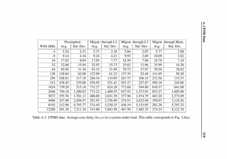
A.C
PMD
Data
114
Preemption Migrat. through L2 Migrat. through L3 Migrat. through Mem.WSS (KB) Avg. Std. Dev. Avg. Std. Dev. Avg. Std. Dev. Avg. Std. Dev.
4 5.24 2.31 5.37 2.36 5.66 2.07 5.77 2.088 9.14 4.18 9.24 4.21 9.93 3.69 10.09 3.82
16 17.02 8.04 17.05 7.77 18.58 7.00 18.78 7.1832 32.88 15.94 32.93 15.73 35.82 13.96 35.99 14.3064 65.05 31.38 65.33 31.90 70.72 27.87 70.50 28.02
128 128.64 62.08 127.09 61.22 137.35 52.48 141.05 58.20256 248.81 117.10 246.34 119.89 267.73 106.19 272.56 115.37512 478.45 239.08 476.95 251.41 507.27 227.87 509.18 245.06
1024 739.20 515.18 733.27 624.26 772.68 544.80 810.37 641.082048 740.10 1,200.93 773.22 1,409.55 837.53 1,373.93 853.27 1,605.603072 355.76 1,781.11 400.88 2,021.39 377.96 1,974.79 483.20 2,373.094096 247.88 2,456.97 291.93 2,756.90 274.51 2,622.08 350.07 3,118.268192 212.90 4,793.77 374.45 5,230.35 436.19 5,153.05 282.28 5,797.23
12288 201.20 7,211.18 333.80 7,683.50 467.50 7,485.35 274.23 8,122.10
Table A.3: CPMD data. Average-case delay (in µs) in a system under load. This table corresponds to Fig. 5.6(a).
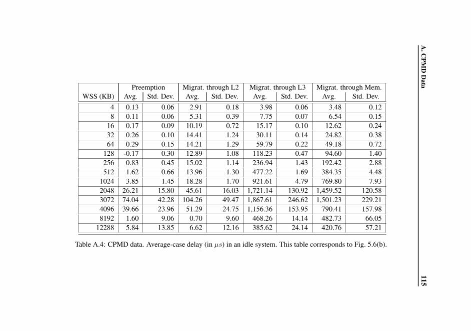
A.C
PMD
Data
115
Preemption Migrat. through L2 Migrat. through L3 Migrat. through Mem.WSS (KB) Avg. Std. Dev. Avg. Std. Dev. Avg. Std. Dev. Avg. Std. Dev.
4 0.13 0.06 2.91 0.18 3.98 0.06 3.48 0.128 0.11 0.06 5.31 0.39 7.75 0.07 6.54 0.15
16 0.17 0.09 10.19 0.72 15.17 0.10 12.62 0.2432 0.26 0.10 14.41 1.24 30.11 0.14 24.82 0.3864 0.29 0.15 14.21 1.29 59.79 0.22 49.18 0.72
128 -0.17 0.30 12.89 1.08 118.23 0.47 94.60 1.40256 0.83 0.45 15.02 1.14 236.94 1.43 192.42 2.88512 1.62 0.66 13.96 1.30 477.22 1.69 384.35 4.48
1024 3.85 1.45 18.28 1.70 921.61 4.79 769.80 7.932048 26.21 15.80 45.61 16.03 1,721.14 130.92 1,459.52 120.583072 74.04 42.28 104.26 49.47 1,867.61 246.62 1,501.23 229.214096 39.66 23.96 51.29 24.75 1,156.36 153.95 790.41 157.988192 1.60 9.06 0.70 9.60 468.26 14.14 482.73 66.05
12288 5.84 13.85 6.62 12.16 385.62 24.14 420.76 57.21
Table A.4: CPMD data. Average-case delay (in µs) in an idle system. This table corresponds to Fig. 5.6(b).

Appendix B
Overheads and Weighted Schedulability Results
for Multiprocessor EDF Scheduling Algorithms
This appendix provides all results in visual form: Sec. B.1 depicts all measured
overheads, and Sec. B.2 presents all weighted schedulability graphs. The extended
online version of [25] also reports all standard schedulability graphs.
B.1 Measured Overheads
The following 6 figures depict measured average and worst-case overheads under
each of the implemented plugins. Note that the y-axis scale varies between graphs.
The overhead graphs are organized as follows.
• Fig. B.1 shows measured scheduling overhead.
• Fig. B.2 shows measured timer re-arming overhead.
• Fig. B.3 shows measured tick overhead.
• Fig. B.4 shows measured context-switching overhead.
• Fig. B.5 shows measured release overhead.
• Fig. B.6 shows measured IPI latency.
116

B.1 Measured Overheads 117
0
50
100
150
200
250
0 50 100 150 200 250 300 350 400
over
head
(us
)
number of tasks
worst-case scheduling overhead
P-EDF G-EDF C-EDF-L2 C-EDF-L3
(a)
0
10
20
30
40
50
60
70
0 50 100 150 200 250 300 350 400
over
head
(us
)
number of tasks
average-case scheduling overhead
P-EDF G-EDF C-EDF-L2 C-EDF-L3
(b)
Figure B.1: Measured scheduling overhead. (a) Measured worst case. (b) Measured aver-age case.

B.1 Measured Overheads 118
0
5
10
15
20
0 50 100 150 200 250 300 350 400
over
head
(us
)
number of tasks
worst-case timer re-arming overhead
P-EDF G-EDF C-EDF-L2 C-EDF-L3
(a)
0
1
2
3
4
5
0 50 100 150 200 250 300 350 400
over
head
(us
)
number of tasks
average-case timer re-arming overhead
P-EDF G-EDF C-EDF-L2 C-EDF-L3
(b)
Figure B.2: Measured timer re-arming overhead. (a) Measured worst case. (b) Measuredaverage case.

B.1 Measured Overheads 119
0
1
2
3
4
5
0 50 100 150 200 250 300 350 400
over
head
(us
)
number of tasks
worst-case tick overhead
P-EDF G-EDF C-EDF-L2 C-EDF-L3
(a)
0
0.5
1
1.5
2
2.5
3
0 50 100 150 200 250 300 350 400
over
head
(us
)
number of tasks
average-case tick overhead
P-EDF G-EDF C-EDF-L2 C-EDF-L3
(b)
Figure B.3: Measured tick overhead. (a) Measured worst case. (b) Measured average case.

B.1 Measured Overheads 120
0
5
10
15
20
0 50 100 150 200 250 300 350 400
over
head
(us
)
number of tasks
worst-case context-switching overhead
P-EDF G-EDF C-EDF-L2 C-EDF-L3
(a)
0
1
2
3
4
5
6
7
8
0 50 100 150 200 250 300 350 400
over
head
(us
)
number of tasks
average-case context-switching overhead
P-EDF G-EDF C-EDF-L2 C-EDF-L3
(b)
Figure B.4: Measured context-switching overhead. (a) Measured worst case. (b) Measuredaverage case.

B.1 Measured Overheads 121
0
50
100
150
200
250
0 50 100 150 200 250 300 350 400
over
head
(us
)
number of tasks
worst-case release overhead
P-EDF G-EDF C-EDF-L2 C-EDF-L3
(a)
0
20
40
60
80
100
0 50 100 150 200 250 300 350 400
over
head
(us
)
number of tasks
average-case release overhead
P-EDF G-EDF C-EDF-L2 C-EDF-L3
(b)
Figure B.5: Measured release overhead. (a) Measured worst case. (b) Measured averagecase.
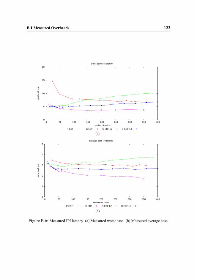
B.1 Measured Overheads 122
0
5
10
15
20
0 50 100 150 200 250 300 350 400
over
head
(us
)
number of tasks
worst-case IPI latency
P-EDF G-EDF C-EDF-L2 C-EDF-L3
(a)
0
1
2
3
4
5
0 50 100 150 200 250 300 350 400
over
head
(us
)
number of tasks
average-case IPI latency
P-EDF G-EDF C-EDF-L2 C-EDF-L3
(b)
Figure B.6: Measured IPI latency. (a) Measured worst case. (b) Measured average case.

B.2 Weighted Schedulability Results 123
B.2 Weighted Schedulability Results
The following 12 figures depict weighted schedulability results for each considered
scenario. They are organized as follows.
• Fig. B.7 shows HRT results for light uniform utilizations under each consid-
ered period distribution.
• Fig. B.8 shows HRT results for medium uniform utilizations under each con-
sidered period distribution.
• Fig. B.9 shows HRT results for heavy uniform utilizations under each consid-
ered period distribution.
• Fig. B.10 shows HRT results for light bimodal utilizations under each consid-
ered period distribution.
• Fig. B.11 shows HRT results for medium bimodal utilizations under each
considered period distribution.
• Fig. B.12 shows HRT results for heavy bimodal utilizations under each con-
sidered period distribution.
• Fig. B.13 shows SRT results for light uniform utilizations under each consid-
ered period distribution.
• Fig. B.14 shows SRT results for medium uniform utilizations under each con-
sidered period distribution.
• Fig. B.15 shows SRT results for heavy uniform utilizations under each con-
sidered period distribution.
• Fig. B.16 shows SRT results for light bimodal utilizations under each consid-
ered period distribution.

B.2 Weighted Schedulability Results 124
• Fig. B.17 shows SRT results for medium bimodal utilizations under each con-
sidered period distribution.
• Fig. B.18 shows SRT results for heavy bimodal utilizations under each con-
sidered period distribution.
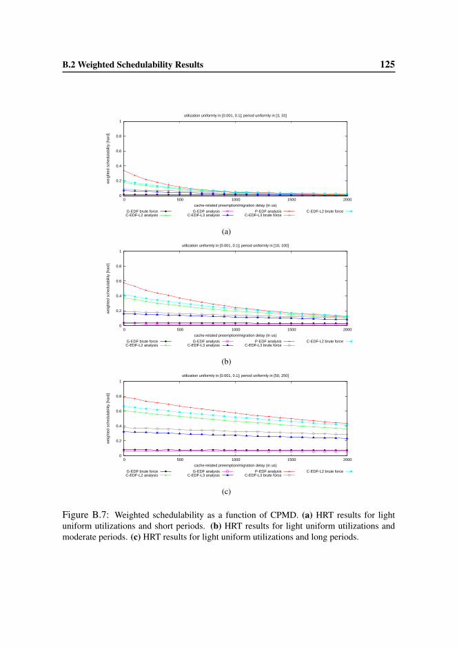
B.2 Weighted Schedulability Results 125
0
0.2
0.4
0.6
0.8
1
0 500 1000 1500 2000
wei
ghte
d sc
hedu
labi
lity
[har
d]
cache-related preemption/migration delay (in us)
utilization uniformly in [0.001, 0.1]; period uniformly in [3, 33]
G-EDF brute forceC-EDF-L2 analysis
G-EDF analysisC-EDF-L3 analysis
P-EDF analysisC-EDF-L3 brute force
C-EDF-L2 brute force
(a)
0
0.2
0.4
0.6
0.8
1
0 500 1000 1500 2000
wei
ghte
d sc
hedu
labi
lity
[har
d]
cache-related preemption/migration delay (in us)
utilization uniformly in [0.001, 0.1]; period uniformly in [10, 100]
G-EDF brute forceC-EDF-L2 analysis
G-EDF analysisC-EDF-L3 analysis
P-EDF analysisC-EDF-L3 brute force
C-EDF-L2 brute force
(b)
0
0.2
0.4
0.6
0.8
1
0 500 1000 1500 2000
wei
ghte
d sc
hedu
labi
lity
[har
d]
cache-related preemption/migration delay (in us)
utilization uniformly in [0.001, 0.1]; period uniformly in [50, 250]
G-EDF brute forceC-EDF-L2 analysis
G-EDF analysisC-EDF-L3 analysis
P-EDF analysisC-EDF-L3 brute force
C-EDF-L2 brute force
(c)
Figure B.7: Weighted schedulability as a function of CPMD. (a) HRT results for lightuniform utilizations and short periods. (b) HRT results for light uniform utilizations andmoderate periods. (c) HRT results for light uniform utilizations and long periods.
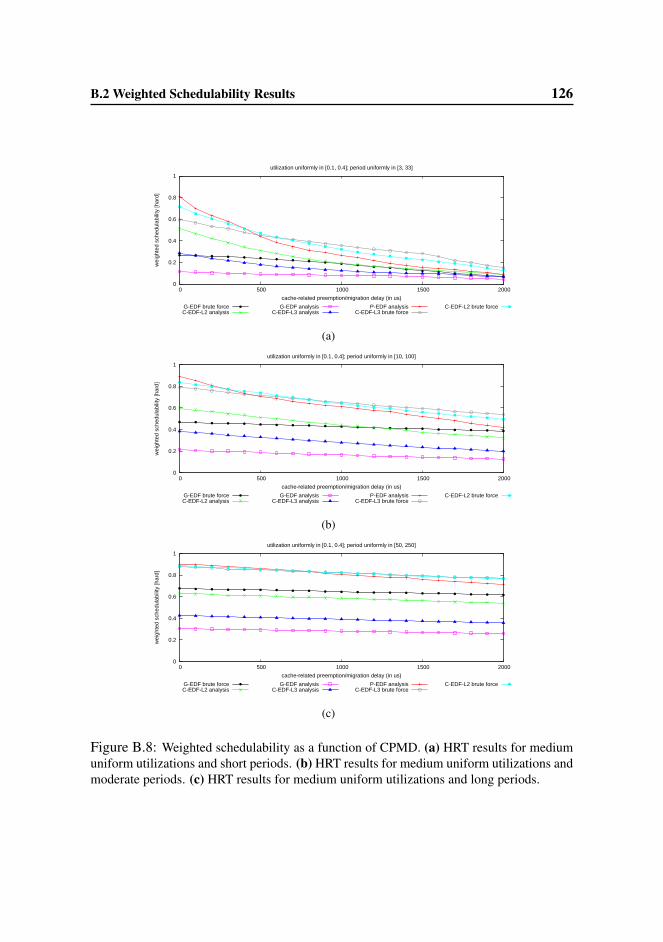
B.2 Weighted Schedulability Results 126
0
0.2
0.4
0.6
0.8
1
0 500 1000 1500 2000
wei
ghte
d sc
hedu
labi
lity
[har
d]
cache-related preemption/migration delay (in us)
utilization uniformly in [0.1, 0.4]; period uniformly in [3, 33]
G-EDF brute forceC-EDF-L2 analysis
G-EDF analysisC-EDF-L3 analysis
P-EDF analysisC-EDF-L3 brute force
C-EDF-L2 brute force
(a)
0
0.2
0.4
0.6
0.8
1
0 500 1000 1500 2000
wei
ghte
d sc
hedu
labi
lity
[har
d]
cache-related preemption/migration delay (in us)
utilization uniformly in [0.1, 0.4]; period uniformly in [10, 100]
G-EDF brute forceC-EDF-L2 analysis
G-EDF analysisC-EDF-L3 analysis
P-EDF analysisC-EDF-L3 brute force
C-EDF-L2 brute force
(b)
0
0.2
0.4
0.6
0.8
1
0 500 1000 1500 2000
wei
ghte
d sc
hedu
labi
lity
[har
d]
cache-related preemption/migration delay (in us)
utilization uniformly in [0.1, 0.4]; period uniformly in [50, 250]
G-EDF brute forceC-EDF-L2 analysis
G-EDF analysisC-EDF-L3 analysis
P-EDF analysisC-EDF-L3 brute force
C-EDF-L2 brute force
(c)
Figure B.8: Weighted schedulability as a function of CPMD. (a) HRT results for mediumuniform utilizations and short periods. (b) HRT results for medium uniform utilizations andmoderate periods. (c) HRT results for medium uniform utilizations and long periods.

B.2 Weighted Schedulability Results 127
0
0.2
0.4
0.6
0.8
1
0 500 1000 1500 2000
wei
ghte
d sc
hedu
labi
lity
[har
d]
cache-related preemption/migration delay (in us)
utilization uniformly in [0.5, 0.9]; period uniformly in [3, 33]
G-EDF brute forceC-EDF-L2 analysis
G-EDF analysisC-EDF-L3 analysis
P-EDF analysisC-EDF-L3 brute force
C-EDF-L2 brute force
(a)
0
0.2
0.4
0.6
0.8
1
0 500 1000 1500 2000
wei
ghte
d sc
hedu
labi
lity
[har
d]
cache-related preemption/migration delay (in us)
utilization uniformly in [0.5, 0.9]; period uniformly in [10, 100]
G-EDF brute forceC-EDF-L2 analysis
G-EDF analysisC-EDF-L3 analysis
P-EDF analysisC-EDF-L3 brute force
C-EDF-L2 brute force
(b)
0
0.2
0.4
0.6
0.8
1
0 500 1000 1500 2000
wei
ghte
d sc
hedu
labi
lity
[har
d]
cache-related preemption/migration delay (in us)
utilization uniformly in [0.5, 0.9]; period uniformly in [50, 250]
G-EDF brute forceC-EDF-L2 analysis
G-EDF analysisC-EDF-L3 analysis
P-EDF analysisC-EDF-L3 brute force
C-EDF-L2 brute force
(c)
Figure B.9: Weighted schedulability as a function of CPMD. (a) HRT results for heavyuniform utilizations and short periods. (b) HRT results for heavy uniform utilizations andmoderate periods. (c) HRT results for heavy uniform utilizations and long periods.

B.2 Weighted Schedulability Results 128
0
0.2
0.4
0.6
0.8
1
0 500 1000 1500 2000
wei
ghte
d sc
hedu
labi
lity
[har
d]
cache-related preemption/migration delay (in us)
util. bimodially in [0.001, 0.5] (8/9) and [0.5, 0.9] (1/9); period uniformly in [3, 33]
G-EDF brute forceC-EDF-L2 analysis
G-EDF analysisC-EDF-L3 analysis
P-EDF analysisC-EDF-L3 brute force
C-EDF-L2 brute force
(a)
0
0.2
0.4
0.6
0.8
1
0 500 1000 1500 2000
wei
ghte
d sc
hedu
labi
lity
[har
d]
cache-related preemption/migration delay (in us)
util. bimodially in [0.001, 0.5] (8/9) and [0.5, 0.9] (1/9); period uniformly in [10, 100]
G-EDF brute forceC-EDF-L2 analysis
G-EDF analysisC-EDF-L3 analysis
P-EDF analysisC-EDF-L3 brute force
C-EDF-L2 brute force
(b)
0
0.2
0.4
0.6
0.8
1
0 500 1000 1500 2000
wei
ghte
d sc
hedu
labi
lity
[har
d]
cache-related preemption/migration delay (in us)
util. bimodially in [0.001, 0.5] (8/9) and [0.5, 0.9] (1/9); period uniformly in [50, 250]
G-EDF brute forceC-EDF-L2 analysis
G-EDF analysisC-EDF-L3 analysis
P-EDF analysisC-EDF-L3 brute force
C-EDF-L2 brute force
(c)
Figure B.10: Weighted schedulability as a function of CPMD. (a) HRT results for lightbimodal utilizations and short periods. (b) HRT results for light bimodal utilizations andmoderate periods. (c) HRT results for light bimodal utilizations and long periods.

B.2 Weighted Schedulability Results 129
0
0.2
0.4
0.6
0.8
1
0 500 1000 1500 2000
wei
ghte
d sc
hedu
labi
lity
[har
d]
cache-related preemption/migration delay (in us)
util. bimodially in [0.001, 0.5] (6/9) and [0.5, 0.9] (3/9); period uniformly in [3, 33]
G-EDF brute forceC-EDF-L2 analysis
G-EDF analysisC-EDF-L3 analysis
P-EDF analysisC-EDF-L3 brute force
C-EDF-L2 brute force
(a)
0
0.2
0.4
0.6
0.8
1
0 500 1000 1500 2000
wei
ghte
d sc
hedu
labi
lity
[har
d]
cache-related preemption/migration delay (in us)
util. bimodially in [0.001, 0.5] (6/9) and [0.5, 0.9] (3/9); period uniformly in [10, 100]
G-EDF brute forceC-EDF-L2 analysis
G-EDF analysisC-EDF-L3 analysis
P-EDF analysisC-EDF-L3 brute force
C-EDF-L2 brute force
(b)
0
0.2
0.4
0.6
0.8
1
0 500 1000 1500 2000
wei
ghte
d sc
hedu
labi
lity
[har
d]
cache-related preemption/migration delay (in us)
util. bimodially in [0.001, 0.5] (6/9) and [0.5, 0.9] (3/9); period uniformly in [50, 250]
G-EDF brute forceC-EDF-L2 analysis
G-EDF analysisC-EDF-L3 analysis
P-EDF analysisC-EDF-L3 brute force
C-EDF-L2 brute force
(c)
Figure B.11: Weighted schedulability as a function of CPMD. (a) HRT results for mediumbimodal utilizations and short periods. (b) HRT results for medium bimodal utilizations andmoderate periods. (c) HRT results for medium bimodal utilizations and long periods.
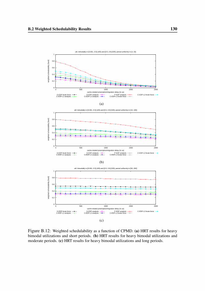
B.2 Weighted Schedulability Results 130
0
0.2
0.4
0.6
0.8
1
0 500 1000 1500 2000
wei
ghte
d sc
hedu
labi
lity
[har
d]
cache-related preemption/migration delay (in us)
util. bimodially in [0.001, 0.5] (4/9) and [0.5, 0.9] (5/9); period uniformly in [3, 33]
G-EDF brute forceC-EDF-L2 analysis
G-EDF analysisC-EDF-L3 analysis
P-EDF analysisC-EDF-L3 brute force
C-EDF-L2 brute force
(a)
0
0.2
0.4
0.6
0.8
1
0 500 1000 1500 2000
wei
ghte
d sc
hedu
labi
lity
[har
d]
cache-related preemption/migration delay (in us)
util. bimodially in [0.001, 0.5] (4/9) and [0.5, 0.9] (5/9); period uniformly in [10, 100]
G-EDF brute forceC-EDF-L2 analysis
G-EDF analysisC-EDF-L3 analysis
P-EDF analysisC-EDF-L3 brute force
C-EDF-L2 brute force
(b)
0
0.2
0.4
0.6
0.8
1
0 500 1000 1500 2000
wei
ghte
d sc
hedu
labi
lity
[har
d]
cache-related preemption/migration delay (in us)
util. bimodially in [0.001, 0.5] (4/9) and [0.5, 0.9] (5/9); period uniformly in [50, 250]
G-EDF brute forceC-EDF-L2 analysis
G-EDF analysisC-EDF-L3 analysis
P-EDF analysisC-EDF-L3 brute force
C-EDF-L2 brute force
(c)
Figure B.12: Weighted schedulability as a function of CPMD. (a) HRT results for heavybimodal utilizations and short periods. (b) HRT results for heavy bimodal utilizations andmoderate periods. (c) HRT results for heavy bimodal utilizations and long periods.

B.2 Weighted Schedulability Results 131
0
0.2
0.4
0.6
0.8
1
0 500 1000 1500 2000
wei
ghte
d sc
hedu
labi
lity
[sof
t]
cache-related preemption/migration delay (in us)
utilization uniformly in [0.001, 0.1]; period uniformly in [3, 33]
G-EDF C-EDF-L3 C-EDF-L2 P-EDF
(a)
0
0.2
0.4
0.6
0.8
1
0 500 1000 1500 2000
wei
ghte
d sc
hedu
labi
lity
[sof
t]
cache-related preemption/migration delay (in us)
utilization uniformly in [0.001, 0.1]; period uniformly in [10, 100]
G-EDF C-EDF-L3 C-EDF-L2 P-EDF
(b)
0
0.2
0.4
0.6
0.8
1
0 500 1000 1500 2000
wei
ghte
d sc
hedu
labi
lity
[sof
t]
cache-related preemption/migration delay (in us)
utilization uniformly in [0.001, 0.1]; period uniformly in [50, 250]
G-EDF C-EDF-L3 C-EDF-L2 P-EDF
(c)
Figure B.13: Weighted schedulability as a function of CPMD. (a) SRT results for lightuniform utilizations and short periods. (b) SRT results for light uniform utilizations andmoderate periods. (c) SRT results for light uniform utilizations and long periods.
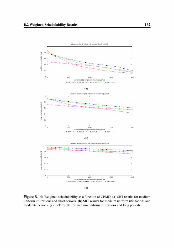
B.2 Weighted Schedulability Results 132
0
0.2
0.4
0.6
0.8
1
0 500 1000 1500 2000
wei
ghte
d sc
hedu
labi
lity
[sof
t]
cache-related preemption/migration delay (in us)
utilization uniformly in [0.1, 0.4]; period uniformly in [3, 33]
G-EDF C-EDF-L3 C-EDF-L2 P-EDF
(a)
0
0.2
0.4
0.6
0.8
1
0 500 1000 1500 2000
wei
ghte
d sc
hedu
labi
lity
[sof
t]
cache-related preemption/migration delay (in us)
utilization uniformly in [0.1, 0.4]; period uniformly in [10, 100]
G-EDF C-EDF-L3 C-EDF-L2 P-EDF
(b)
0
0.2
0.4
0.6
0.8
1
0 500 1000 1500 2000
wei
ghte
d sc
hedu
labi
lity
[sof
t]
cache-related preemption/migration delay (in us)
utilization uniformly in [0.1, 0.4]; period uniformly in [50, 250]
G-EDF C-EDF-L3 C-EDF-L2 P-EDF
(c)
Figure B.14: Weighted schedulability as a function of CPMD. (a) SRT results for mediumuniform utilizations and short periods. (b) SRT results for medium uniform utilizations andmoderate periods. (c) SRT results for medium uniform utilizations and long periods.

B.2 Weighted Schedulability Results 133
0
0.2
0.4
0.6
0.8
1
0 500 1000 1500 2000
wei
ghte
d sc
hedu
labi
lity
[sof
t]
cache-related preemption/migration delay (in us)
utilization uniformly in [0.5, 0.9]; period uniformly in [3, 33]
G-EDF C-EDF-L3 C-EDF-L2 P-EDF
(a)
0
0.2
0.4
0.6
0.8
1
0 500 1000 1500 2000
wei
ghte
d sc
hedu
labi
lity
[sof
t]
cache-related preemption/migration delay (in us)
utilization uniformly in [0.5, 0.9]; period uniformly in [10, 100]
G-EDF C-EDF-L3 C-EDF-L2 P-EDF
(b)
0
0.2
0.4
0.6
0.8
1
0 500 1000 1500 2000
wei
ghte
d sc
hedu
labi
lity
[sof
t]
cache-related preemption/migration delay (in us)
utilization uniformly in [0.5, 0.9]; period uniformly in [50, 250]
G-EDF C-EDF-L3 C-EDF-L2 P-EDF
(c)
Figure B.15: Weighted schedulability as a function of CPMD. (a) SRT results for heavyuniform utilizations and short periods. (b) SRT results for heavy uniform utilizations andmoderate periods. (c) SRT results for heavy uniform utilizations and long periods.
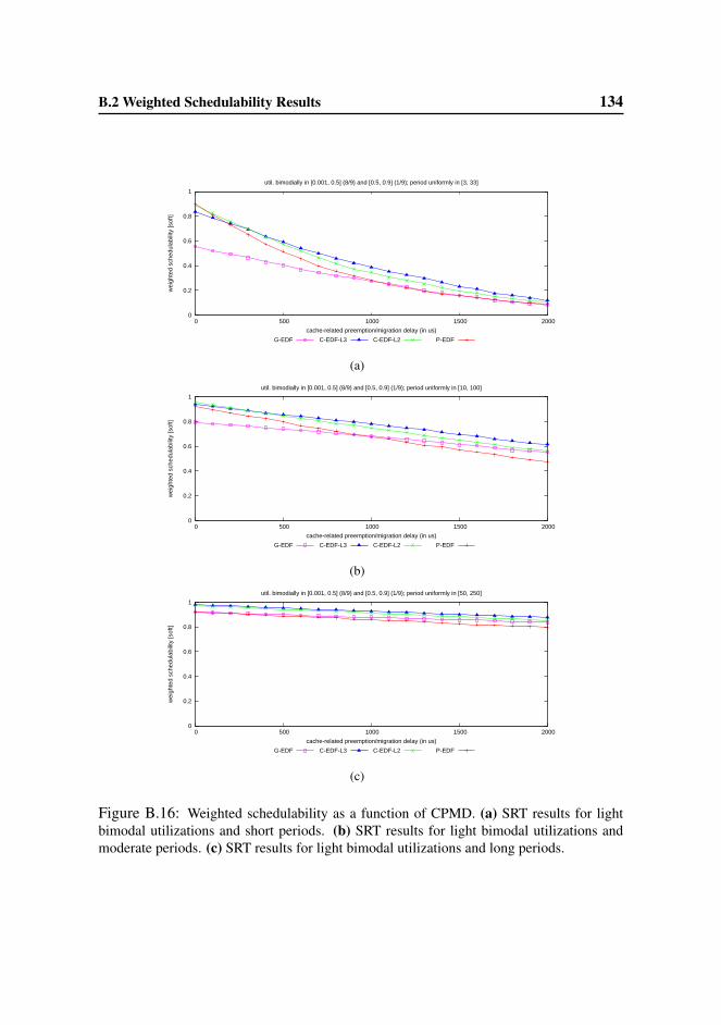
B.2 Weighted Schedulability Results 134
0
0.2
0.4
0.6
0.8
1
0 500 1000 1500 2000
wei
ghte
d sc
hedu
labi
lity
[sof
t]
cache-related preemption/migration delay (in us)
util. bimodially in [0.001, 0.5] (8/9) and [0.5, 0.9] (1/9); period uniformly in [3, 33]
G-EDF C-EDF-L3 C-EDF-L2 P-EDF
(a)
0
0.2
0.4
0.6
0.8
1
0 500 1000 1500 2000
wei
ghte
d sc
hedu
labi
lity
[sof
t]
cache-related preemption/migration delay (in us)
util. bimodially in [0.001, 0.5] (8/9) and [0.5, 0.9] (1/9); period uniformly in [10, 100]
G-EDF C-EDF-L3 C-EDF-L2 P-EDF
(b)
0
0.2
0.4
0.6
0.8
1
0 500 1000 1500 2000
wei
ghte
d sc
hedu
labi
lity
[sof
t]
cache-related preemption/migration delay (in us)
util. bimodially in [0.001, 0.5] (8/9) and [0.5, 0.9] (1/9); period uniformly in [50, 250]
G-EDF C-EDF-L3 C-EDF-L2 P-EDF
(c)
Figure B.16: Weighted schedulability as a function of CPMD. (a) SRT results for lightbimodal utilizations and short periods. (b) SRT results for light bimodal utilizations andmoderate periods. (c) SRT results for light bimodal utilizations and long periods.
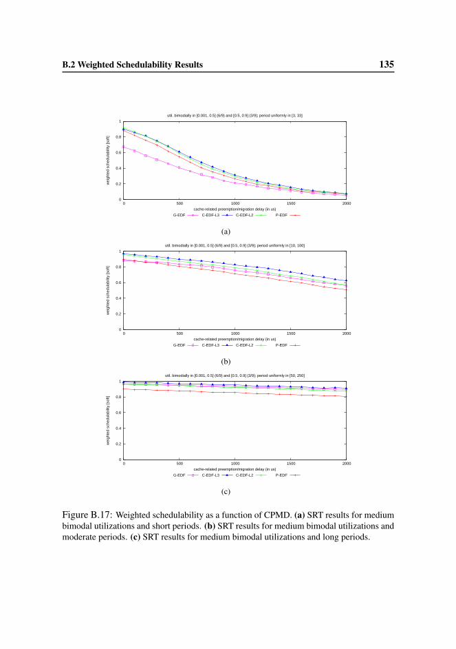
B.2 Weighted Schedulability Results 135
0
0.2
0.4
0.6
0.8
1
0 500 1000 1500 2000
wei
ghte
d sc
hedu
labi
lity
[sof
t]
cache-related preemption/migration delay (in us)
util. bimodially in [0.001, 0.5] (6/9) and [0.5, 0.9] (3/9); period uniformly in [3, 33]
G-EDF C-EDF-L3 C-EDF-L2 P-EDF
(a)
0
0.2
0.4
0.6
0.8
1
0 500 1000 1500 2000
wei
ghte
d sc
hedu
labi
lity
[sof
t]
cache-related preemption/migration delay (in us)
util. bimodially in [0.001, 0.5] (6/9) and [0.5, 0.9] (3/9); period uniformly in [10, 100]
G-EDF C-EDF-L3 C-EDF-L2 P-EDF
(b)
0
0.2
0.4
0.6
0.8
1
0 500 1000 1500 2000
wei
ghte
d sc
hedu
labi
lity
[sof
t]
cache-related preemption/migration delay (in us)
util. bimodially in [0.001, 0.5] (6/9) and [0.5, 0.9] (3/9); period uniformly in [50, 250]
G-EDF C-EDF-L3 C-EDF-L2 P-EDF
(c)
Figure B.17: Weighted schedulability as a function of CPMD. (a) SRT results for mediumbimodal utilizations and short periods. (b) SRT results for medium bimodal utilizations andmoderate periods. (c) SRT results for medium bimodal utilizations and long periods.
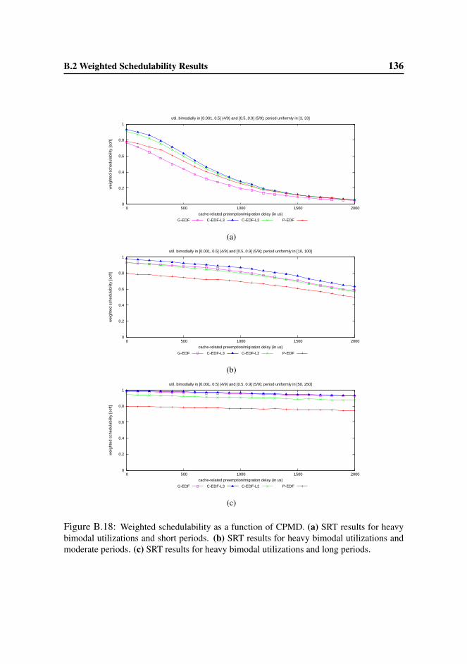
B.2 Weighted Schedulability Results 136
0
0.2
0.4
0.6
0.8
1
0 500 1000 1500 2000
wei
ghte
d sc
hedu
labi
lity
[sof
t]
cache-related preemption/migration delay (in us)
util. bimodially in [0.001, 0.5] (4/9) and [0.5, 0.9] (5/9); period uniformly in [3, 33]
G-EDF C-EDF-L3 C-EDF-L2 P-EDF
(a)
0
0.2
0.4
0.6
0.8
1
0 500 1000 1500 2000
wei
ghte
d sc
hedu
labi
lity
[sof
t]
cache-related preemption/migration delay (in us)
util. bimodially in [0.001, 0.5] (4/9) and [0.5, 0.9] (5/9); period uniformly in [10, 100]
G-EDF C-EDF-L3 C-EDF-L2 P-EDF
(b)
0
0.2
0.4
0.6
0.8
1
0 500 1000 1500 2000
wei
ghte
d sc
hedu
labi
lity
[sof
t]
cache-related preemption/migration delay (in us)
util. bimodially in [0.001, 0.5] (4/9) and [0.5, 0.9] (5/9); period uniformly in [50, 250]
G-EDF C-EDF-L3 C-EDF-L2 P-EDF
(c)
Figure B.18: Weighted schedulability as a function of CPMD. (a) SRT results for heavybimodal utilizations and short periods. (b) SRT results for heavy bimodal utilizations andmoderate periods. (c) SRT results for heavy bimodal utilizations and long periods.

Appendix C
Overheads and Weighted Schedulability Results
for Semi-partitioned Algorithms
This appendix provides all results in visual form: Sec. C.1 depicts all measured
overheads, and Sec. C.2 presents all weighted schedulability graphs for ξ ≤ 1024
KB. The extended online version of [26] also reports weighted schedulability graphs
for the full range of WSS, and all standard schedulability graphs.
C.1 Measured Overheads
The following 6 figures depict measured average and worst-case overheads under
each of the implemented plugins. Note that the y-axis scale varies between graphs.
The overhead graphs are organized as follows.
• Fig. C.1 shows measured scheduling overhead.
• Fig. C.2 shows measured timer re-arming overhead.
• Fig. C.3 shows measured tick overhead.
• Fig. C.4 shows measured context-switching overhead.
• Fig. C.5 shows measured release overhead.
137
C.1 Measured Overheads 138
• Fig. C.6 shows measured IPI latency.

C.1 Measured Overheads 139
0
5
10
15
20
25
30
0 50 100 150 200 250 300 350
overh
ead (
us)
number of tasks
worst-case scheduling overhead
C-EDF C-NPS-F EDF-fm EDF-WM NPS-F P-EDF
(a)
0
5
10
15
20
0 50 100 150 200 250 300 350
overh
ead (
us)
number of tasks
average-case scheduling overhead
C-EDF C-NPS-F EDF-fm EDF-WM NPS-F P-EDF
(b)
Figure C.1: Measured scheduling overhead. (a) Measured worst case. (b) Measured aver-age case.

C.1 Measured Overheads 140
0
5
10
15
20
25
30
35
0 50 100 150 200 250 300 350
overh
ead (
us)
number of tasks
worst-case timer re-arming overhead
C-EDF C-NPS-F EDF-fm EDF-WM NPS-F P-EDF
(a)
0
2
4
6
8
10
0 50 100 150 200 250 300 350
overh
ead (
us)
number of tasks
average-case timer re-arming overhead
C-EDF C-NPS-F EDF-fm EDF-WM NPS-F P-EDF
(b)
Figure C.2: Measured timer re-arming overhead. (a) Measured worst case. (b) Measuredaverage case.

C.1 Measured Overheads 141
0
1
2
3
4
5
0 50 100 150 200 250 300 350
overh
ead (
us)
number of tasks
worst-case tick overhead
C-EDF C-NPS-F EDF-fm EDF-WM NPS-F P-EDF
(a)
0
0.5
1
1.5
2
2.5
3
0 50 100 150 200 250 300 350
overh
ead (
us)
number of tasks
average-case tick overhead
C-EDF C-NPS-F EDF-fm EDF-WM NPS-F P-EDF
(b)
Figure C.3: Measured tick overhead. (a) Measured worst case. (b) Measured average case.

C.1 Measured Overheads 142
0
5
10
15
20
0 50 100 150 200 250 300 350
overh
ead (
us)
number of tasks
worst-case context-switching overhead
C-EDF C-NPS-F EDF-fm EDF-WM NPS-F P-EDF
(a)
0
1
2
3
4
5
6
7
8
0 50 100 150 200 250 300 350
overh
ead (
us)
number of tasks
average-case context-switching overhead
C-EDF C-NPS-F EDF-fm EDF-WM NPS-F P-EDF
(b)
Figure C.4: Measured context-switching overhead. (a) Measured worst case. (b) Measuredaverage case.
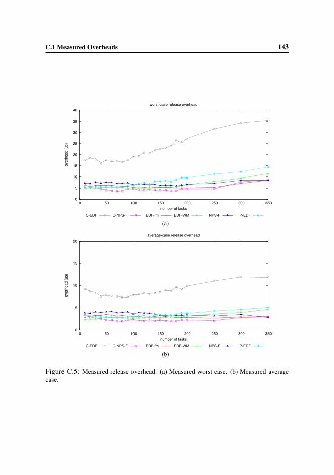
C.1 Measured Overheads 143
0
5
10
15
20
25
30
35
40
0 50 100 150 200 250 300 350
overh
ead (
us)
number of tasks
worst-case release overhead
C-EDF C-NPS-F EDF-fm EDF-WM NPS-F P-EDF
(a)
0
5
10
15
20
0 50 100 150 200 250 300 350
overh
ead (
us)
number of tasks
average-case release overhead
C-EDF C-NPS-F EDF-fm EDF-WM NPS-F P-EDF
(b)
Figure C.5: Measured release overhead. (a) Measured worst case. (b) Measured averagecase.

C.1 Measured Overheads 144
0
5
10
15
20
25
30
35
0 50 100 150 200 250 300 350
overh
ead (
us)
number of tasks
worst-case IPI latency
C-EDF C-NPS-F EDF-fm EDF-WM NPS-F P-EDF
(a)
0
2
4
6
8
10
0 50 100 150 200 250 300 350
overh
ead (
us)
number of tasks
average-case IPI latency
C-EDF C-NPS-F EDF-fm EDF-WM NPS-F P-EDF
(b)
Figure C.6: Measured IPI latency. (a) Measured worst case. (b) Measured average case.

C.2 Weighted Schedulability Results 145
C.2 Weighted Schedulability Results
The following 18 figures depict weighted schedulability results for each considered
scenario. They are organized as follows.
• Fig. C.7 shows HRT results for light uniform utilizations under each consid-
ered period distribution for ξ ≤ 1024 KB.
• Fig. C.8 shows HRT results for medium uniform utilizations under each con-
sidered period distribution for ξ ≤ 1024 KB.
• Fig. C.9 shows HRT results for heavy uniform utilizations under each consid-
ered period distribution for ξ ≤ 1024 KB.
• Fig. C.10 shows HRT results for light bimodal utilizations under each consid-
ered period distribution for ξ ≤ 1024 KB.
• Fig. C.11 shows HRT results for medium bimodal utilizations under each
considered period distribution for ξ ≤ 1024 KB.
• Fig. C.12 shows HRT results for heavy bimodal utilizations under each con-
sidered period distribution for ξ ≤ 1024 KB.
• Fig. C.13 shows HRT results for light exponential utilizations under each con-
sidered period distribution for ξ ≤ 1024 KB.
• Fig. C.14 shows HRT results for medium exponential utilizations under each
considered period distribution for ξ ≤ 1024 KB.
• Fig. C.15 shows HRT results for heavy exponential utilizations under each
considered period distribution for ξ ≤ 1024 KB.
• Fig. C.16 shows SRT results for light uniform utilizations under each consid-
ered period distribution for ξ ≤ 1024 KB.
C.2 Weighted Schedulability Results 146
• Fig. C.17 shows SRT results for medium uniform utilizations under each con-
sidered period distribution for ξ ≤ 1024 KB.
• Fig. C.18 shows SRT results for heavy uniform utilizations under each con-
sidered period distribution for ξ ≤ 1024 KB.
• Fig. C.19 shows SRT results for light bimodal utilizations under each consid-
ered period distribution for ξ ≤ 1024 KB.
• Fig. C.20 shows SRT results for medium bimodal utilizations under each con-
sidered period distribution for ξ ≤ 1024 KB.
• Fig. C.21 shows SRT results for heavy bimodal utilizations under each con-
sidered period distribution for ξ ≤ 1024 KB.
• Fig. C.22 shows SRT results for light exponential utilizations under each con-
sidered period distribution for ξ ≤ 1024 KB.
• Fig. C.23 shows SRT results for medium exponential utilizations under each
considered period distribution for ξ ≤ 1024 KB.
• Fig. C.24 shows SRT results for heavy exponential utilizations under each
considered period distribution for ξ ≤ 1024 KB.
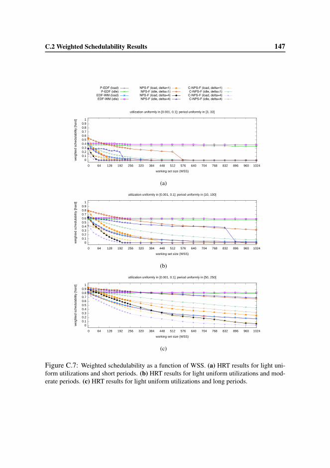
C.2 Weighted Schedulability Results 147
0 0.1 0.2 0.3 0.4 0.5 0.6 0.7 0.8 0.9
1
1 2 3 4 5 6 7 8 9 10 11 12 13 14 15 16 17 18 19 20 21 22 23 24
ratio
of s
ched
ulab
le ta
sk s
ets
[har
d]
task set utilization cap (prior to overhead accounting)
util. bimodally in [0.001, 0.5] (4/9) and [0.5, 0.9] (5/9); period uniformly in [3, 33]; WSS = 48kB
P-EDF (load)P-EDF (idle)
EDF-WM (load)EDF-WM (idle)
NPS-F (load, delta=1)NPS-F (idle, delta=1)
NPS-F (load, delta=4)NPS-F (idle, delta=4)
C-NPS-F (load, delta=1)C-NPS-F (idle, delta=1)
C-NPS-F (load, delta=4)C-NPS-F (idle, delta=4)
0 0.1 0.2 0.3 0.4 0.5 0.6 0.7 0.8 0.9
1
0 64 128 192 256 320 384 448 512 576 640 704 768 832 896 960 1024
wei
ghte
d sc
hedu
labi
lity
[har
d]
working set size (WSS)
utilization uniformly in [0.001, 0.1]; period uniformly in [3, 33]
(a)
0 0.1 0.2 0.3 0.4 0.5 0.6 0.7 0.8 0.9
1
0 64 128 192 256 320 384 448 512 576 640 704 768 832 896 960 1024
wei
ghte
d sc
hedu
labi
lity
[har
d]
working set size (WSS)
utilization uniformly in [0.001, 0.1]; period uniformly in [10, 100]
(b)
0 0.1 0.2 0.3 0.4 0.5 0.6 0.7 0.8 0.9
1
0 64 128 192 256 320 384 448 512 576 640 704 768 832 896 960 1024
wei
ghte
d sc
hedu
labi
lity
[har
d]
working set size (WSS)
utilization uniformly in [0.001, 0.1]; period uniformly in [50, 250]
(c)
Figure C.7: Weighted schedulability as a function of WSS. (a) HRT results for light uni-form utilizations and short periods. (b) HRT results for light uniform utilizations and mod-erate periods. (c) HRT results for light uniform utilizations and long periods.
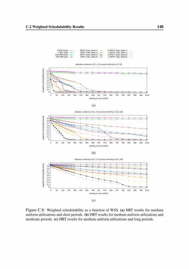
C.2 Weighted Schedulability Results 148
0 0.1 0.2 0.3 0.4 0.5 0.6 0.7 0.8 0.9
1
1 2 3 4 5 6 7 8 9 10 11 12 13 14 15 16 17 18 19 20 21 22 23 24
ratio
of s
ched
ulab
le ta
sk s
ets
[har
d]
task set utilization cap (prior to overhead accounting)
util. bimodally in [0.001, 0.5] (4/9) and [0.5, 0.9] (5/9); period uniformly in [3, 33]; WSS = 48kB
P-EDF (load)P-EDF (idle)
EDF-WM (load)EDF-WM (idle)
NPS-F (load, delta=1)NPS-F (idle, delta=1)
NPS-F (load, delta=4)NPS-F (idle, delta=4)
C-NPS-F (load, delta=1)C-NPS-F (idle, delta=1)
C-NPS-F (load, delta=4)C-NPS-F (idle, delta=4)
0 0.1 0.2 0.3 0.4 0.5 0.6 0.7 0.8 0.9
1
0 64 128 192 256 320 384 448 512 576 640 704 768 832 896 960 1024
wei
ghte
d sc
hedu
labi
lity
[har
d]
working set size (WSS)
utilization uniformly in [0.1, 0.4]; period uniformly in [3, 33]
(a)
0 0.1 0.2 0.3 0.4 0.5 0.6 0.7 0.8 0.9
1
0 64 128 192 256 320 384 448 512 576 640 704 768 832 896 960 1024
wei
ghte
d sc
hedu
labi
lity
[har
d]
working set size (WSS)
utilization uniformly in [0.1, 0.4]; period uniformly in [10, 100]
(b)
0 0.1 0.2 0.3 0.4 0.5 0.6 0.7 0.8 0.9
1
0 64 128 192 256 320 384 448 512 576 640 704 768 832 896 960 1024
wei
ghte
d sc
hedu
labi
lity
[har
d]
working set size (WSS)
utilization uniformly in [0.1, 0.4]; period uniformly in [50, 250]
(c)
Figure C.8: Weighted schedulability as a function of WSS. (a) HRT results for mediumuniform utilizations and short periods. (b) HRT results for medium uniform utilizations andmoderate periods. (c) HRT results for medium uniform utilizations and long periods.

C.2 Weighted Schedulability Results 149
0 0.1 0.2 0.3 0.4 0.5 0.6 0.7 0.8 0.9
1
1 2 3 4 5 6 7 8 9 10 11 12 13 14 15 16 17 18 19 20 21 22 23 24
ratio
of s
ched
ulab
le ta
sk s
ets
[har
d]
task set utilization cap (prior to overhead accounting)
util. bimodally in [0.001, 0.5] (4/9) and [0.5, 0.9] (5/9); period uniformly in [3, 33]; WSS = 48kB
P-EDF (load)P-EDF (idle)
EDF-WM (load)EDF-WM (idle)
NPS-F (load, delta=1)NPS-F (idle, delta=1)
NPS-F (load, delta=4)NPS-F (idle, delta=4)
C-NPS-F (load, delta=1)C-NPS-F (idle, delta=1)
C-NPS-F (load, delta=4)C-NPS-F (idle, delta=4)
0 0.1 0.2 0.3 0.4 0.5 0.6 0.7 0.8 0.9
1
0 64 128 192 256 320 384 448 512 576 640 704 768 832 896 960 1024
wei
ghte
d sc
hedu
labi
lity
[har
d]
working set size (WSS)
utilization uniformly in [0.5, 0.9]; period uniformly in [3, 33]
(a)
0 0.1 0.2 0.3 0.4 0.5 0.6 0.7 0.8 0.9
1
0 64 128 192 256 320 384 448 512 576 640 704 768 832 896 960 1024
wei
ghte
d sc
hedu
labi
lity
[har
d]
working set size (WSS)
utilization uniformly in [0.5, 0.9]; period uniformly in [10, 100]
(b)
0 0.1 0.2 0.3 0.4 0.5 0.6 0.7 0.8 0.9
1
0 64 128 192 256 320 384 448 512 576 640 704 768 832 896 960 1024
wei
ghte
d sc
hedu
labi
lity
[har
d]
working set size (WSS)
utilization uniformly in [0.5, 0.9]; period uniformly in [50, 250]
(c)
Figure C.9: Weighted schedulability as a function of WSS. (a) HRT results for heavyuniform utilizations and short periods. (b) HRT results for heavy uniform utilizations andmoderate periods. (c) HRT results for heavy uniform utilizations and long periods.
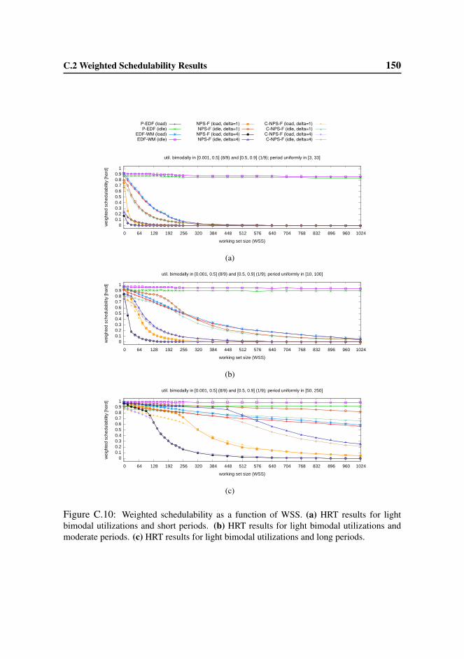
C.2 Weighted Schedulability Results 150
0 0.1 0.2 0.3 0.4 0.5 0.6 0.7 0.8 0.9
1
1 2 3 4 5 6 7 8 9 10 11 12 13 14 15 16 17 18 19 20 21 22 23 24
ratio
of s
ched
ulab
le ta
sk s
ets
[har
d]
task set utilization cap (prior to overhead accounting)
util. bimodally in [0.001, 0.5] (4/9) and [0.5, 0.9] (5/9); period uniformly in [3, 33]; WSS = 48kB
P-EDF (load)P-EDF (idle)
EDF-WM (load)EDF-WM (idle)
NPS-F (load, delta=1)NPS-F (idle, delta=1)
NPS-F (load, delta=4)NPS-F (idle, delta=4)
C-NPS-F (load, delta=1)C-NPS-F (idle, delta=1)
C-NPS-F (load, delta=4)C-NPS-F (idle, delta=4)
0 0.1 0.2 0.3 0.4 0.5 0.6 0.7 0.8 0.9
1
0 64 128 192 256 320 384 448 512 576 640 704 768 832 896 960 1024
wei
ghte
d sc
hedu
labi
lity
[har
d]
working set size (WSS)
util. bimodally in [0.001, 0.5] (8/9) and [0.5, 0.9] (1/9); period uniformly in [3, 33]
(a)
0 0.1 0.2 0.3 0.4 0.5 0.6 0.7 0.8 0.9
1
0 64 128 192 256 320 384 448 512 576 640 704 768 832 896 960 1024
wei
ghte
d sc
hedu
labi
lity
[har
d]
working set size (WSS)
util. bimodally in [0.001, 0.5] (8/9) and [0.5, 0.9] (1/9); period uniformly in [10, 100]
(b)
0 0.1 0.2 0.3 0.4 0.5 0.6 0.7 0.8 0.9
1
0 64 128 192 256 320 384 448 512 576 640 704 768 832 896 960 1024
wei
ghte
d sc
hedu
labi
lity
[har
d]
working set size (WSS)
util. bimodally in [0.001, 0.5] (8/9) and [0.5, 0.9] (1/9); period uniformly in [50, 250]
(c)
Figure C.10: Weighted schedulability as a function of WSS. (a) HRT results for lightbimodal utilizations and short periods. (b) HRT results for light bimodal utilizations andmoderate periods. (c) HRT results for light bimodal utilizations and long periods.
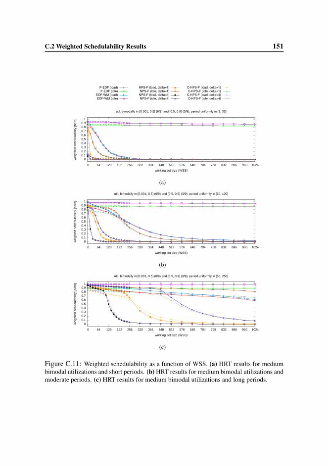
C.2 Weighted Schedulability Results 151
0 0.1 0.2 0.3 0.4 0.5 0.6 0.7 0.8 0.9
1
1 2 3 4 5 6 7 8 9 10 11 12 13 14 15 16 17 18 19 20 21 22 23 24
ratio
of s
ched
ulab
le ta
sk s
ets
[har
d]
task set utilization cap (prior to overhead accounting)
util. bimodally in [0.001, 0.5] (4/9) and [0.5, 0.9] (5/9); period uniformly in [3, 33]; WSS = 48kB
P-EDF (load)P-EDF (idle)
EDF-WM (load)EDF-WM (idle)
NPS-F (load, delta=1)NPS-F (idle, delta=1)
NPS-F (load, delta=4)NPS-F (idle, delta=4)
C-NPS-F (load, delta=1)C-NPS-F (idle, delta=1)
C-NPS-F (load, delta=4)C-NPS-F (idle, delta=4)
0 0.1 0.2 0.3 0.4 0.5 0.6 0.7 0.8 0.9
1
0 64 128 192 256 320 384 448 512 576 640 704 768 832 896 960 1024
wei
ghte
d sc
hedu
labi
lity
[har
d]
working set size (WSS)
util. bimodally in [0.001, 0.5] (6/9) and [0.5, 0.9] (3/9); period uniformly in [3, 33]
(a)
0 0.1 0.2 0.3 0.4 0.5 0.6 0.7 0.8 0.9
1
0 64 128 192 256 320 384 448 512 576 640 704 768 832 896 960 1024
wei
ghte
d sc
hedu
labi
lity
[har
d]
working set size (WSS)
util. bimodally in [0.001, 0.5] (6/9) and [0.5, 0.9] (3/9); period uniformly in [10, 100]
(b)
0 0.1 0.2 0.3 0.4 0.5 0.6 0.7 0.8 0.9
1
0 64 128 192 256 320 384 448 512 576 640 704 768 832 896 960 1024
wei
ghte
d sc
hedu
labi
lity
[har
d]
working set size (WSS)
util. bimodally in [0.001, 0.5] (6/9) and [0.5, 0.9] (3/9); period uniformly in [50, 250]
(c)
Figure C.11: Weighted schedulability as a function of WSS. (a) HRT results for mediumbimodal utilizations and short periods. (b) HRT results for medium bimodal utilizations andmoderate periods. (c) HRT results for medium bimodal utilizations and long periods.

C.2 Weighted Schedulability Results 152
0 0.1 0.2 0.3 0.4 0.5 0.6 0.7 0.8 0.9
1
1 2 3 4 5 6 7 8 9 10 11 12 13 14 15 16 17 18 19 20 21 22 23 24
ratio
of s
ched
ulab
le ta
sk s
ets
[har
d]
task set utilization cap (prior to overhead accounting)
util. bimodally in [0.001, 0.5] (4/9) and [0.5, 0.9] (5/9); period uniformly in [3, 33]; WSS = 48kB
P-EDF (load)P-EDF (idle)
EDF-WM (load)EDF-WM (idle)
NPS-F (load, delta=1)NPS-F (idle, delta=1)
NPS-F (load, delta=4)NPS-F (idle, delta=4)
C-NPS-F (load, delta=1)C-NPS-F (idle, delta=1)
C-NPS-F (load, delta=4)C-NPS-F (idle, delta=4)
0 0.1 0.2 0.3 0.4 0.5 0.6 0.7 0.8 0.9
1
0 64 128 192 256 320 384 448 512 576 640 704 768 832 896 960 1024
wei
ghte
d sc
hedu
labi
lity
[har
d]
working set size (WSS)
util. bimodally in [0.001, 0.5] (4/9) and [0.5, 0.9] (5/9); period uniformly in [3, 33]
(a)
0 0.1 0.2 0.3 0.4 0.5 0.6 0.7 0.8 0.9
1
0 64 128 192 256 320 384 448 512 576 640 704 768 832 896 960 1024
wei
ghte
d sc
hedu
labi
lity
[har
d]
working set size (WSS)
util. bimodally in [0.001, 0.5] (4/9) and [0.5, 0.9] (5/9); period uniformly in [10, 100]
(b)
0 0.1 0.2 0.3 0.4 0.5 0.6 0.7 0.8 0.9
1
0 64 128 192 256 320 384 448 512 576 640 704 768 832 896 960 1024
wei
ghte
d sc
hedu
labi
lity
[har
d]
working set size (WSS)
util. bimodally in [0.001, 0.5] (4/9) and [0.5, 0.9] (5/9); period uniformly in [50, 250]
(c)
Figure C.12: Weighted schedulability as a function of WSS. (a) HRT results for heavybimodal utilizations and short periods. (b) HRT results for heavy bimodal utilizations andmoderate periods. (c) HRT results for heavy bimodal utilizations and long periods.

C.2 Weighted Schedulability Results 153
0 0.1 0.2 0.3 0.4 0.5 0.6 0.7 0.8 0.9
1
1 2 3 4 5 6 7 8 9 10 11 12 13 14 15 16 17 18 19 20 21 22 23 24
ratio
of s
ched
ulab
le ta
sk s
ets
[har
d]
task set utilization cap (prior to overhead accounting)
util. bimodally in [0.001, 0.5] (4/9) and [0.5, 0.9] (5/9); period uniformly in [3, 33]; WSS = 48kB
P-EDF (load)P-EDF (idle)
EDF-WM (load)EDF-WM (idle)
NPS-F (load, delta=1)NPS-F (idle, delta=1)
NPS-F (load, delta=4)NPS-F (idle, delta=4)
C-NPS-F (load, delta=1)C-NPS-F (idle, delta=1)
C-NPS-F (load, delta=4)C-NPS-F (idle, delta=4)
0 0.1 0.2 0.3 0.4 0.5 0.6 0.7 0.8 0.9
1
0 64 128 192 256 320 384 448 512 576 640 704 768 832 896 960 1024
wei
ghte
d sc
hedu
labi
lity
[har
d]
working set size (WSS)
util. exponentially in [0, 1] with mean 0.10; period uniformly in [3, 33]
(a)
0 0.1 0.2 0.3 0.4 0.5 0.6 0.7 0.8 0.9
1
0 64 128 192 256 320 384 448 512 576 640 704 768 832 896 960 1024
wei
ghte
d sc
hedu
labi
lity
[har
d]
working set size (WSS)
util. exponentially in [0, 1] with mean 0.10; period uniformly in [10, 100]
(b)
0 0.1 0.2 0.3 0.4 0.5 0.6 0.7 0.8 0.9
1
0 64 128 192 256 320 384 448 512 576 640 704 768 832 896 960 1024
wei
ghte
d sc
hedu
labi
lity
[har
d]
working set size (WSS)
util. exponentially in [0, 1] with mean 0.10; period uniformly in [50, 250]
(c)
Figure C.13: Weighted schedulability as a function of WSS. (a) HRT results for lightexponential utilizations and short periods. (b) HRT results for light exponential utilizationsand moderate periods. (c) HRT results for light exponential utilizations and long periods.

C.2 Weighted Schedulability Results 154
0 0.1 0.2 0.3 0.4 0.5 0.6 0.7 0.8 0.9
1
1 2 3 4 5 6 7 8 9 10 11 12 13 14 15 16 17 18 19 20 21 22 23 24
ratio
of s
ched
ulab
le ta
sk s
ets
[har
d]
task set utilization cap (prior to overhead accounting)
util. bimodally in [0.001, 0.5] (4/9) and [0.5, 0.9] (5/9); period uniformly in [3, 33]; WSS = 48kB
P-EDF (load)P-EDF (idle)
EDF-WM (load)EDF-WM (idle)
NPS-F (load, delta=1)NPS-F (idle, delta=1)
NPS-F (load, delta=4)NPS-F (idle, delta=4)
C-NPS-F (load, delta=1)C-NPS-F (idle, delta=1)
C-NPS-F (load, delta=4)C-NPS-F (idle, delta=4)
0 0.1 0.2 0.3 0.4 0.5 0.6 0.7 0.8 0.9
1
0 64 128 192 256 320 384 448 512 576 640 704 768 832 896 960 1024
wei
ghte
d sc
hedu
labi
lity
[har
d]
working set size (WSS)
util. exponentially in [0, 1] with mean 0.25; period uniformly in [3, 33]
(a)
0 0.1 0.2 0.3 0.4 0.5 0.6 0.7 0.8 0.9
1
0 64 128 192 256 320 384 448 512 576 640 704 768 832 896 960 1024
wei
ghte
d sc
hedu
labi
lity
[har
d]
working set size (WSS)
util. exponentially in [0, 1] with mean 0.25; period uniformly in [10, 100]
(b)
0 0.1 0.2 0.3 0.4 0.5 0.6 0.7 0.8 0.9
1
0 64 128 192 256 320 384 448 512 576 640 704 768 832 896 960 1024
wei
ghte
d sc
hedu
labi
lity
[har
d]
working set size (WSS)
util. exponentially in [0, 1] with mean 0.25; period uniformly in [50, 250]
(c)
Figure C.14: Weighted schedulability as a function of WSS. (a) HRT results for mediumexponential utilizations and short periods. (b) HRT results for medium exponential utiliza-tions and moderate periods. (c) HRT results for medium exponential utilizations and longperiods.
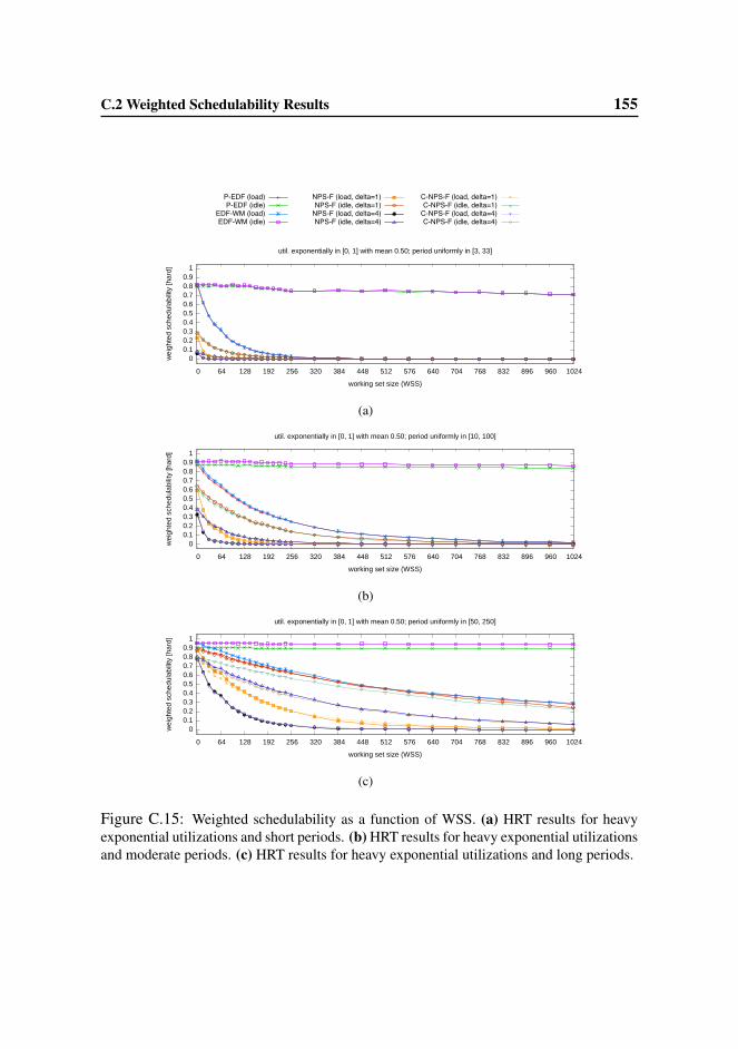
C.2 Weighted Schedulability Results 155
0 0.1 0.2 0.3 0.4 0.5 0.6 0.7 0.8 0.9
1
1 2 3 4 5 6 7 8 9 10 11 12 13 14 15 16 17 18 19 20 21 22 23 24
ratio
of s
ched
ulab
le ta
sk s
ets
[har
d]
task set utilization cap (prior to overhead accounting)
util. bimodally in [0.001, 0.5] (4/9) and [0.5, 0.9] (5/9); period uniformly in [3, 33]; WSS = 48kB
P-EDF (load)P-EDF (idle)
EDF-WM (load)EDF-WM (idle)
NPS-F (load, delta=1)NPS-F (idle, delta=1)
NPS-F (load, delta=4)NPS-F (idle, delta=4)
C-NPS-F (load, delta=1)C-NPS-F (idle, delta=1)
C-NPS-F (load, delta=4)C-NPS-F (idle, delta=4)
0 0.1 0.2 0.3 0.4 0.5 0.6 0.7 0.8 0.9
1
0 64 128 192 256 320 384 448 512 576 640 704 768 832 896 960 1024
wei
ghte
d sc
hedu
labi
lity
[har
d]
working set size (WSS)
util. exponentially in [0, 1] with mean 0.50; period uniformly in [3, 33]
(a)
0 0.1 0.2 0.3 0.4 0.5 0.6 0.7 0.8 0.9
1
0 64 128 192 256 320 384 448 512 576 640 704 768 832 896 960 1024
wei
ghte
d sc
hedu
labi
lity
[har
d]
working set size (WSS)
util. exponentially in [0, 1] with mean 0.50; period uniformly in [10, 100]
(b)
0 0.1 0.2 0.3 0.4 0.5 0.6 0.7 0.8 0.9
1
0 64 128 192 256 320 384 448 512 576 640 704 768 832 896 960 1024
wei
ghte
d sc
hedu
labi
lity
[har
d]
working set size (WSS)
util. exponentially in [0, 1] with mean 0.50; period uniformly in [50, 250]
(c)
Figure C.15: Weighted schedulability as a function of WSS. (a) HRT results for heavyexponential utilizations and short periods. (b) HRT results for heavy exponential utilizationsand moderate periods. (c) HRT results for heavy exponential utilizations and long periods.

C.2 Weighted Schedulability Results 156
0 0.1 0.2 0.3 0.4 0.5 0.6 0.7 0.8 0.9
1
1 2 3 4 5 6 7 8 9 10 11 12 13 14 15 16 17 18 19 20 21 22 23 24
ratio
of s
ched
ulab
le ta
sk s
ets
[sof
t]
task set utilization cap (prior to overhead accounting)
util. bimodally in [0.001, 0.5] (8/9) and [0.5, 0.9] (1/9); period uniformly in [3, 33]; WSS = 16kB
C-EDF (load)C-EDF (idle)
EDF-WM (load)EDF-WM (idle)
NPS-F (load, delta=1)
NPS-F (idle, delta=1)NPS-F (load, delta=4)NPS-F (idle, delta=4)
C-NPS-F (load, delta=1)C-NPS-F (idle, delta=1)
C-NPS-F (load, delta=4)C-NPS-F (idle, delta=4)
EDF-fm (load)EDF-fm (idle)
0 0.1 0.2 0.3 0.4 0.5 0.6 0.7 0.8 0.9
1
0 64 128 192 256 320 384 448 512 576 640 704 768 832 896 960 1024
wei
ghte
d sc
hedu
labi
lity
[sof
t]
working set size (WSS)
utilization uniformly in [0.001, 0.1]; period uniformly in [3, 33]
(a)
0 0.1 0.2 0.3 0.4 0.5 0.6 0.7 0.8 0.9
1
0 64 128 192 256 320 384 448 512 576 640 704 768 832 896 960 1024
wei
ghte
d sc
hedu
labi
lity
[sof
t]
working set size (WSS)
utilization uniformly in [0.001, 0.1]; period uniformly in [10, 100]
(b)
0 0.1 0.2 0.3 0.4 0.5 0.6 0.7 0.8 0.9
1
0 64 128 192 256 320 384 448 512 576 640 704 768 832 896 960 1024
wei
ghte
d sc
hedu
labi
lity
[sof
t]
working set size (WSS)
utilization uniformly in [0.001, 0.1]; period uniformly in [50, 250]
(c)
Figure C.16: Weighted schedulability as a function of WSS. (a) SRT results for lightuniform utilizations and short periods. (b) SRT results for light uniform utilizations andmoderate periods. (c) SRT results for light uniform utilizations and long periods.
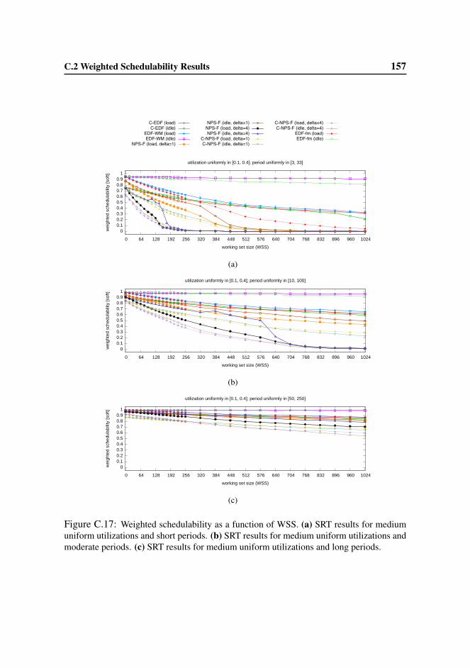
C.2 Weighted Schedulability Results 157
0 0.1 0.2 0.3 0.4 0.5 0.6 0.7 0.8 0.9
1
1 2 3 4 5 6 7 8 9 10 11 12 13 14 15 16 17 18 19 20 21 22 23 24
ratio
of s
ched
ulab
le ta
sk s
ets
[sof
t]
task set utilization cap (prior to overhead accounting)
util. bimodally in [0.001, 0.5] (8/9) and [0.5, 0.9] (1/9); period uniformly in [3, 33]; WSS = 16kB
C-EDF (load)C-EDF (idle)
EDF-WM (load)EDF-WM (idle)
NPS-F (load, delta=1)
NPS-F (idle, delta=1)NPS-F (load, delta=4)NPS-F (idle, delta=4)
C-NPS-F (load, delta=1)C-NPS-F (idle, delta=1)
C-NPS-F (load, delta=4)C-NPS-F (idle, delta=4)
EDF-fm (load)EDF-fm (idle)
0 0.1 0.2 0.3 0.4 0.5 0.6 0.7 0.8 0.9
1
0 64 128 192 256 320 384 448 512 576 640 704 768 832 896 960 1024
wei
ghte
d sc
hedu
labi
lity
[sof
t]
working set size (WSS)
utilization uniformly in [0.1, 0.4]; period uniformly in [3, 33]
(a)
0 0.1 0.2 0.3 0.4 0.5 0.6 0.7 0.8 0.9
1
0 64 128 192 256 320 384 448 512 576 640 704 768 832 896 960 1024
wei
ghte
d sc
hedu
labi
lity
[sof
t]
working set size (WSS)
utilization uniformly in [0.1, 0.4]; period uniformly in [10, 100]
(b)
0 0.1 0.2 0.3 0.4 0.5 0.6 0.7 0.8 0.9
1
0 64 128 192 256 320 384 448 512 576 640 704 768 832 896 960 1024
wei
ghte
d sc
hedu
labi
lity
[sof
t]
working set size (WSS)
utilization uniformly in [0.1, 0.4]; period uniformly in [50, 250]
(c)
Figure C.17: Weighted schedulability as a function of WSS. (a) SRT results for mediumuniform utilizations and short periods. (b) SRT results for medium uniform utilizations andmoderate periods. (c) SRT results for medium uniform utilizations and long periods.

C.2 Weighted Schedulability Results 158
0 0.1 0.2 0.3 0.4 0.5 0.6 0.7 0.8 0.9
1
1 2 3 4 5 6 7 8 9 10 11 12 13 14 15 16 17 18 19 20 21 22 23 24
ratio
of s
ched
ulab
le ta
sk s
ets
[sof
t]
task set utilization cap (prior to overhead accounting)
util. bimodally in [0.001, 0.5] (8/9) and [0.5, 0.9] (1/9); period uniformly in [3, 33]; WSS = 16kB
C-EDF (load)C-EDF (idle)
EDF-WM (load)EDF-WM (idle)
NPS-F (load, delta=1)
NPS-F (idle, delta=1)NPS-F (load, delta=4)NPS-F (idle, delta=4)
C-NPS-F (load, delta=1)C-NPS-F (idle, delta=1)
C-NPS-F (load, delta=4)C-NPS-F (idle, delta=4)
EDF-fm (load)EDF-fm (idle)
0 0.1 0.2 0.3 0.4 0.5 0.6 0.7 0.8 0.9
1
0 64 128 192 256 320 384 448 512 576 640 704 768 832 896 960 1024
wei
ghte
d sc
hedu
labi
lity
[sof
t]
working set size (WSS)
utilization uniformly in [0.5, 0.9]; period uniformly in [3, 33]
(a)
0 0.1 0.2 0.3 0.4 0.5 0.6 0.7 0.8 0.9
1
0 64 128 192 256 320 384 448 512 576 640 704 768 832 896 960 1024
wei
ghte
d sc
hedu
labi
lity
[sof
t]
working set size (WSS)
utilization uniformly in [0.5, 0.9]; period uniformly in [10, 100]
(b)
0 0.1 0.2 0.3 0.4 0.5 0.6 0.7 0.8 0.9
1
0 64 128 192 256 320 384 448 512 576 640 704 768 832 896 960 1024
wei
ghte
d sc
hedu
labi
lity
[sof
t]
working set size (WSS)
utilization uniformly in [0.5, 0.9]; period uniformly in [50, 250]
(c)
Figure C.18: Weighted schedulability as a function of WSS. (a) SRT results for heavyuniform utilizations and short periods. (b) SRT results for heavy uniform utilizations andmoderate periods. (c) SRT results for heavy uniform utilizations and long periods.

C.2 Weighted Schedulability Results 159
0 0.1 0.2 0.3 0.4 0.5 0.6 0.7 0.8 0.9
1
1 2 3 4 5 6 7 8 9 10 11 12 13 14 15 16 17 18 19 20 21 22 23 24
ratio
of s
ched
ulab
le ta
sk s
ets
[sof
t]
task set utilization cap (prior to overhead accounting)
util. bimodally in [0.001, 0.5] (8/9) and [0.5, 0.9] (1/9); period uniformly in [3, 33]; WSS = 16kB
C-EDF (load)C-EDF (idle)
EDF-WM (load)EDF-WM (idle)
NPS-F (load, delta=1)
NPS-F (idle, delta=1)NPS-F (load, delta=4)NPS-F (idle, delta=4)
C-NPS-F (load, delta=1)C-NPS-F (idle, delta=1)
C-NPS-F (load, delta=4)C-NPS-F (idle, delta=4)
EDF-fm (load)EDF-fm (idle)
0 0.1 0.2 0.3 0.4 0.5 0.6 0.7 0.8 0.9
1
0 64 128 192 256 320 384 448 512 576 640 704 768 832 896 960 1024
wei
ghte
d sc
hedu
labi
lity
[sof
t]
working set size (WSS)
util. bimodally in [0.001, 0.5] (8/9) and [0.5, 0.9] (1/9); period uniformly in [3, 33]
(a)
0 0.1 0.2 0.3 0.4 0.5 0.6 0.7 0.8 0.9
1
0 64 128 192 256 320 384 448 512 576 640 704 768 832 896 960 1024
wei
ghte
d sc
hedu
labi
lity
[sof
t]
working set size (WSS)
util. bimodally in [0.001, 0.5] (8/9) and [0.5, 0.9] (1/9); period uniformly in [10, 100]
(b)
0 0.1 0.2 0.3 0.4 0.5 0.6 0.7 0.8 0.9
1
0 64 128 192 256 320 384 448 512 576 640 704 768 832 896 960 1024
wei
ghte
d sc
hedu
labi
lity
[sof
t]
working set size (WSS)
util. bimodally in [0.001, 0.5] (8/9) and [0.5, 0.9] (1/9); period uniformly in [50, 250]
(c)
Figure C.19: Weighted schedulability as a function of WSS. (a) SRT results for lightbimodal utilizations and short periods. (b) SRT results for light bimodal utilizations andmoderate periods. (c) SRT results for light bimodal utilizations and long periods.

C.2 Weighted Schedulability Results 160
0 0.1 0.2 0.3 0.4 0.5 0.6 0.7 0.8 0.9
1
1 2 3 4 5 6 7 8 9 10 11 12 13 14 15 16 17 18 19 20 21 22 23 24
ratio
of s
ched
ulab
le ta
sk s
ets
[sof
t]
task set utilization cap (prior to overhead accounting)
util. bimodally in [0.001, 0.5] (8/9) and [0.5, 0.9] (1/9); period uniformly in [3, 33]; WSS = 16kB
C-EDF (load)C-EDF (idle)
EDF-WM (load)EDF-WM (idle)
NPS-F (load, delta=1)
NPS-F (idle, delta=1)NPS-F (load, delta=4)NPS-F (idle, delta=4)
C-NPS-F (load, delta=1)C-NPS-F (idle, delta=1)
C-NPS-F (load, delta=4)C-NPS-F (idle, delta=4)
EDF-fm (load)EDF-fm (idle)
0 0.1 0.2 0.3 0.4 0.5 0.6 0.7 0.8 0.9
1
0 64 128 192 256 320 384 448 512 576 640 704 768 832 896 960 1024
wei
ghte
d sc
hedu
labi
lity
[sof
t]
working set size (WSS)
util. bimodally in [0.001, 0.5] (6/9) and [0.5, 0.9] (3/9); period uniformly in [3, 33]
(a)
0 0.1 0.2 0.3 0.4 0.5 0.6 0.7 0.8 0.9
1
0 64 128 192 256 320 384 448 512 576 640 704 768 832 896 960 1024
wei
ghte
d sc
hedu
labi
lity
[sof
t]
working set size (WSS)
util. bimodally in [0.001, 0.5] (6/9) and [0.5, 0.9] (3/9); period uniformly in [10, 100]
(b)
0 0.1 0.2 0.3 0.4 0.5 0.6 0.7 0.8 0.9
1
0 64 128 192 256 320 384 448 512 576 640 704 768 832 896 960 1024
wei
ghte
d sc
hedu
labi
lity
[sof
t]
working set size (WSS)
util. bimodally in [0.001, 0.5] (6/9) and [0.5, 0.9] (3/9); period uniformly in [50, 250]
(c)
Figure C.20: Weighted schedulability as a function of WSS. (a) SRT results for mediumbimodal utilizations and short periods. (b) SRT results for medium bimodal utilizations andmoderate periods. (c) SRT results for medium bimodal utilizations and long periods.

C.2 Weighted Schedulability Results 161
0 0.1 0.2 0.3 0.4 0.5 0.6 0.7 0.8 0.9
1
1 2 3 4 5 6 7 8 9 10 11 12 13 14 15 16 17 18 19 20 21 22 23 24
ratio
of s
ched
ulab
le ta
sk s
ets
[sof
t]
task set utilization cap (prior to overhead accounting)
util. bimodally in [0.001, 0.5] (8/9) and [0.5, 0.9] (1/9); period uniformly in [3, 33]; WSS = 16kB
C-EDF (load)C-EDF (idle)
EDF-WM (load)EDF-WM (idle)
NPS-F (load, delta=1)
NPS-F (idle, delta=1)NPS-F (load, delta=4)NPS-F (idle, delta=4)
C-NPS-F (load, delta=1)C-NPS-F (idle, delta=1)
C-NPS-F (load, delta=4)C-NPS-F (idle, delta=4)
EDF-fm (load)EDF-fm (idle)
0 0.1 0.2 0.3 0.4 0.5 0.6 0.7 0.8 0.9
1
0 64 128 192 256 320 384 448 512 576 640 704 768 832 896 960 1024
wei
ghte
d sc
hedu
labi
lity
[sof
t]
working set size (WSS)
util. bimodally in [0.001, 0.5] (4/9) and [0.5, 0.9] (5/9); period uniformly in [3, 33]
(a)
0 0.1 0.2 0.3 0.4 0.5 0.6 0.7 0.8 0.9
1
0 64 128 192 256 320 384 448 512 576 640 704 768 832 896 960 1024
wei
ghte
d sc
hedu
labi
lity
[sof
t]
working set size (WSS)
util. bimodally in [0.001, 0.5] (4/9) and [0.5, 0.9] (5/9); period uniformly in [10, 100]
(b)
0 0.1 0.2 0.3 0.4 0.5 0.6 0.7 0.8 0.9
1
0 64 128 192 256 320 384 448 512 576 640 704 768 832 896 960 1024
wei
ghte
d sc
hedu
labi
lity
[sof
t]
working set size (WSS)
util. bimodally in [0.001, 0.5] (4/9) and [0.5, 0.9] (5/9); period uniformly in [50, 250]
(c)
Figure C.21: Weighted schedulability as a function of WSS. (a) SRT results for heavybimodal utilizations and short periods. (b) SRT results for heavy bimodal utilizations andmoderate periods. (c) SRT results for heavy bimodal utilizations and long periods.

C.2 Weighted Schedulability Results 162
0 0.1 0.2 0.3 0.4 0.5 0.6 0.7 0.8 0.9
1
1 2 3 4 5 6 7 8 9 10 11 12 13 14 15 16 17 18 19 20 21 22 23 24
ratio
of s
ched
ulab
le ta
sk s
ets
[sof
t]
task set utilization cap (prior to overhead accounting)
util. bimodally in [0.001, 0.5] (8/9) and [0.5, 0.9] (1/9); period uniformly in [3, 33]; WSS = 16kB
C-EDF (load)C-EDF (idle)
EDF-WM (load)EDF-WM (idle)
NPS-F (load, delta=1)
NPS-F (idle, delta=1)NPS-F (load, delta=4)NPS-F (idle, delta=4)
C-NPS-F (load, delta=1)C-NPS-F (idle, delta=1)
C-NPS-F (load, delta=4)C-NPS-F (idle, delta=4)
EDF-fm (load)EDF-fm (idle)
0 0.1 0.2 0.3 0.4 0.5 0.6 0.7 0.8 0.9
1
0 64 128 192 256 320 384 448 512 576 640 704 768 832 896 960 1024
wei
ghte
d sc
hedu
labi
lity
[sof
t]
working set size (WSS)
util. exponentially in [0, 1] with mean 0.10; period uniformly in [3, 33]
(a)
0 0.1 0.2 0.3 0.4 0.5 0.6 0.7 0.8 0.9
1
0 64 128 192 256 320 384 448 512 576 640 704 768 832 896 960 1024
wei
ghte
d sc
hedu
labi
lity
[sof
t]
working set size (WSS)
util. exponentially in [0, 1] with mean 0.10; period uniformly in [10, 100]
(b)
0 0.1 0.2 0.3 0.4 0.5 0.6 0.7 0.8 0.9
1
0 64 128 192 256 320 384 448 512 576 640 704 768 832 896 960 1024
wei
ghte
d sc
hedu
labi
lity
[sof
t]
working set size (WSS)
util. exponentially in [0, 1] with mean 0.10; period uniformly in [50, 250]
(c)
Figure C.22: Weighted schedulability as a function of WSS. (a) SRT results for lightexponential utilizations and short periods. (b) SRT results for light exponential utilizationsand moderate periods. (c) SRT results for light exponential utilizations and long periods.
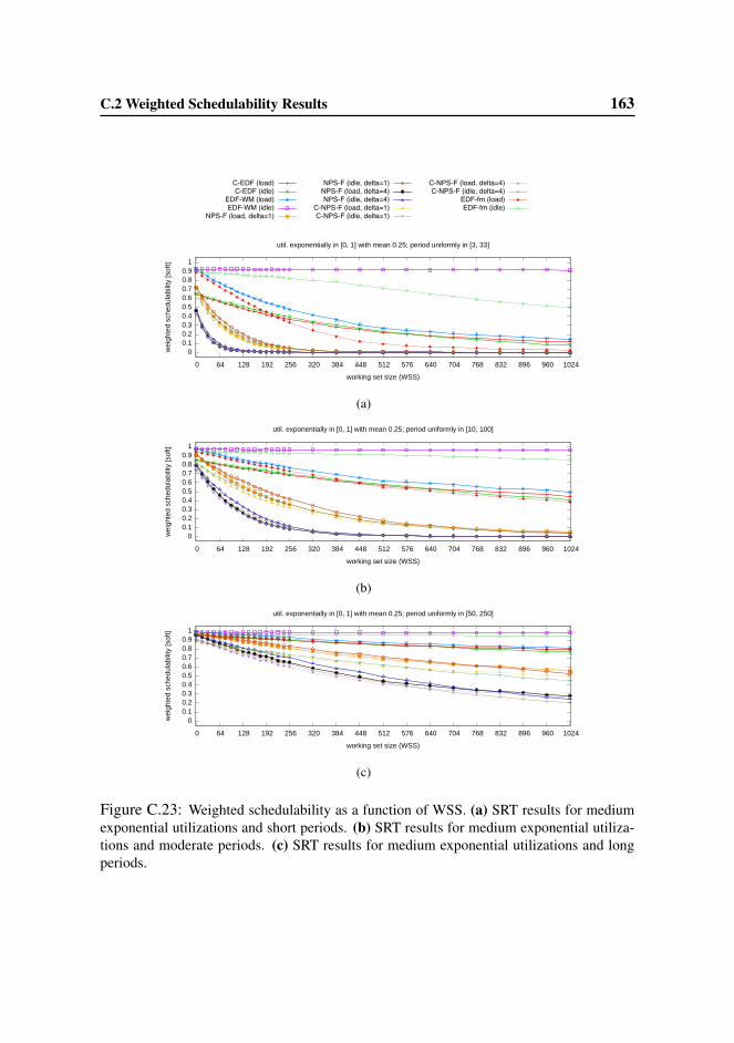
C.2 Weighted Schedulability Results 163
0 0.1 0.2 0.3 0.4 0.5 0.6 0.7 0.8 0.9
1
1 2 3 4 5 6 7 8 9 10 11 12 13 14 15 16 17 18 19 20 21 22 23 24
ratio
of s
ched
ulab
le ta
sk s
ets
[sof
t]
task set utilization cap (prior to overhead accounting)
util. bimodally in [0.001, 0.5] (8/9) and [0.5, 0.9] (1/9); period uniformly in [3, 33]; WSS = 16kB
C-EDF (load)C-EDF (idle)
EDF-WM (load)EDF-WM (idle)
NPS-F (load, delta=1)
NPS-F (idle, delta=1)NPS-F (load, delta=4)NPS-F (idle, delta=4)
C-NPS-F (load, delta=1)C-NPS-F (idle, delta=1)
C-NPS-F (load, delta=4)C-NPS-F (idle, delta=4)
EDF-fm (load)EDF-fm (idle)
0 0.1 0.2 0.3 0.4 0.5 0.6 0.7 0.8 0.9
1
0 64 128 192 256 320 384 448 512 576 640 704 768 832 896 960 1024
wei
ghte
d sc
hedu
labi
lity
[sof
t]
working set size (WSS)
util. exponentially in [0, 1] with mean 0.25; period uniformly in [3, 33]
(a)
0 0.1 0.2 0.3 0.4 0.5 0.6 0.7 0.8 0.9
1
0 64 128 192 256 320 384 448 512 576 640 704 768 832 896 960 1024
wei
ghte
d sc
hedu
labi
lity
[sof
t]
working set size (WSS)
util. exponentially in [0, 1] with mean 0.25; period uniformly in [10, 100]
(b)
0 0.1 0.2 0.3 0.4 0.5 0.6 0.7 0.8 0.9
1
0 64 128 192 256 320 384 448 512 576 640 704 768 832 896 960 1024
wei
ghte
d sc
hedu
labi
lity
[sof
t]
working set size (WSS)
util. exponentially in [0, 1] with mean 0.25; period uniformly in [50, 250]
(c)
Figure C.23: Weighted schedulability as a function of WSS. (a) SRT results for mediumexponential utilizations and short periods. (b) SRT results for medium exponential utiliza-tions and moderate periods. (c) SRT results for medium exponential utilizations and longperiods.

C.2 Weighted Schedulability Results 164
0 0.1 0.2 0.3 0.4 0.5 0.6 0.7 0.8 0.9
1
1 2 3 4 5 6 7 8 9 10 11 12 13 14 15 16 17 18 19 20 21 22 23 24
ratio
of s
ched
ulab
le ta
sk s
ets
[sof
t]
task set utilization cap (prior to overhead accounting)
util. bimodally in [0.001, 0.5] (8/9) and [0.5, 0.9] (1/9); period uniformly in [3, 33]; WSS = 16kB
C-EDF (load)C-EDF (idle)
EDF-WM (load)EDF-WM (idle)
NPS-F (load, delta=1)
NPS-F (idle, delta=1)NPS-F (load, delta=4)NPS-F (idle, delta=4)
C-NPS-F (load, delta=1)C-NPS-F (idle, delta=1)
C-NPS-F (load, delta=4)C-NPS-F (idle, delta=4)
EDF-fm (load)EDF-fm (idle)
0 0.1 0.2 0.3 0.4 0.5 0.6 0.7 0.8 0.9
1
0 64 128 192 256 320 384 448 512 576 640 704 768 832 896 960 1024
wei
ghte
d sc
hedu
labi
lity
[sof
t]
working set size (WSS)
util. exponentially in [0, 1] with mean 0.50; period uniformly in [3, 33]
(a)
0 0.1 0.2 0.3 0.4 0.5 0.6 0.7 0.8 0.9
1
0 64 128 192 256 320 384 448 512 576 640 704 768 832 896 960 1024
wei
ghte
d sc
hedu
labi
lity
[sof
t]
working set size (WSS)
util. exponentially in [0, 1] with mean 0.50; period uniformly in [10, 100]
(b)
0 0.1 0.2 0.3 0.4 0.5 0.6 0.7 0.8 0.9
1
0 64 128 192 256 320 384 448 512 576 640 704 768 832 896 960 1024
wei
ghte
d sc
hedu
labi
lity
[sof
t]
working set size (WSS)
util. exponentially in [0, 1] with mean 0.50; period uniformly in [50, 250]
(c)
Figure C.24: Weighted schedulability as a function of WSS. (a) SRT results for heavyexponential utilizations and short periods. (b) SRT results for heavy exponential utilizationsand moderate periods. (c) SRT results for heavy exponential utilizations and long periods.

Bibliography
[1] L. Abeni and G. Buttazzo. Integrating multimedia applications in hard real-
time systems. In Proc. of the 19th IEEE Real-Time Sys. Symp., pp. 4–13,
1998.
[2] L. Abeni and Giorgio C. Buttazzo. Resource reservation in dynamic real-time
systems. Real-Time Syst., 27:123–167, July 2004.
[3] A. Agarwal, J. Hennessy, and M. Horowitz. An analytical cache model. ACM
Trans. on Computer Sys., 7(2):184–215, 1989.
[4] Airlines Electronic Engineering Commitee. ARINC Specication 653-1 -
Avionics Application Software Standard Interface, 2006.
[5] J. Anderson, V. Bud, and U. Devi. An EDF-based scheduling algorithm for
multiprocessor soft real-time systems. In Proc. of the 17th Euromicro Conf.
on Real-Time Sys., pp. 199–208, 2005.
[6] J. Anderson, V. Bud, and U. Devi. An EDF-based restricted-migration
scheduling algorithm for multiprocessor soft real-time systems. Real-Time
Syst., 38:85–131, 2008.
[7] J. Anderson and A. Srinivasan. Mixed Pfair/ERfair scheduling of asyn-
chronous periodic tasks. Journal of Computer and System Sciences, 68:157–
204, February 2004.
165

Bibliography 166
[8] B. Andersson and K. Bletsas. Sporadic multiprocessor scheduling with few
preemptions. In Proc. of the 20th Euromicro Conf. on Real-Time Sys., pp.
243–252, 2008.
[9] B. Andersson, K. Bletsas, and S. Baruah. Scheduling arbitrary-deadline spo-
radic task systems on multiprocessors. In Proc. of the 29th IEEE Real-Time
Sys. Symp., pp. 385–394, 2008.
[10] B. Andersson and J. Jonsson. The utilization bounds of partitioned and pfair
static-priority scheduling on multiprocessors are 50%. In Proc. of the 15th
Euromicro Conf. on Real-Time Sys., page 33. 2003.
[11] B. Andersson and L. Pinho. Implementing multicore real-time scheduling al-
gorithms based on task splitting using Ada 2012. In Reliable Software Tech-
nologiey – Ada-Europe 2010, volume 6106 of Lecture Notes in Computer
Science, pp. 54–67. Springer Berlin / Heidelberg, 2010.
[12] B. Andersson and E. Tovar. Multiprocessor scheduling with few preemptions.
In Proc. of the 12th IEEE Int’l Conf. on Embedded and Real-Time Computing
Sys. and Apps., pp. 322–334, 2006.
[13] B. Andersson, E. Tovar, and P. B. Sousa. Implementing slot-based task-
splitting multiprocessor scheduling. Technical Report HURRAY-TR-100504,
IPP Hurray!, May 2010.
[14] Ars Technica, Conde Nast Digital. Ext4 filesystem hits Android, no
need to fear data loss. http://arstechnica.com/open-source/news/2010/12/
ext4-filesystem-hits-android-no-need-to-fear-data-loss.ars. Accessed:
12/29/2010.
[15] A. Atlas and A. Bestavros. Statistical rate monotonic scheduling. In Proc. of
the 19th IEEE Real-Time Sys. Symp., pp. 123–, 1998.

Bibliography 167
[16] T. Baker. Stack-based scheduling for realtime processes. Real-Time Syst.,
3:67–99, April 1991.
[17] T. Baker. Multiprocessor EDF and deadline monotonic schedulability analy-
sis. In Proc. of the 24th IEEE Real-Time Sys. Symp., pp. 120–129, 2003.
[18] T. Baker. A comparison of global and partitioned EDF schedulability tests
for multiprocessors. Technical Report TR-051101, Florida State University,
2005.
[19] T. Baker and S. Baruah. Schedulability analysis of multiprocessor sporadic
task systems. In Handbook of Real-Time and Embedded Sys.. Chapman
Hall/CRC, 2007.
[20] S. Baruah. Techniques for multiprocessor global schedulability analysis. In
Proc. of the 28th IEEE Real-Time Sys. Symp., pp. 119–128, 2007.
[21] S. Baruah, N. K. Cohen, C. G. Plaxton, and D. A. Varvel. Proportion-
ate progress: A notion of fairness in resource allocation. Algorithmica,
15(6):600–625, 1996.
[22] S. K. Baruah. Optimal utilization bounds for the fixed-priority scheduling
of periodic task systems on identical multiprocessors. IEEE Trans. Comput.,
53:781–784, June 2004.
[23] A. Bastoni, B. Brandenburg, and J. Anderson. An empirical
comparison of global, partitioned, and clustered multiprocessor
EDF schedulers. Extended version of the paper. Available at
http:// www.cs.unc.edu/ ˜anderson/papers.html.
[24] A. Bastoni, B. Brandenburg, and J. Anderson. Cache-related preemption and
migration delays: Empirical approximation and impact on schedulability. In
Proc. of the 6th Int’l Workshop on Operating Sys. Platforms for Embedded
Real-Time Apps., pp. 33–44, 2010.

Bibliography 168
[25] A. Bastoni, B. Brandenburg, and J. Anderson. An empirical comparison of
global, partitioned, and clustered multiprocessor EDF schedulers. In Proc. of
the 31st IEEE Real-Time Sys. Symp., pp. 14–24, 2010.
[26] A. Bastoni, B. Brandenburg, and J. Anderson. Is semi-partitioned scheduling
practical? In Proc. of the 23nd Euromicro Conf. on Real-Time Sys., 2011.
Accepted for publication. The extended version of the paper is available at
http:// www.cs.unc.edu/ ˜anderson/papers.html.
[27] S. Basumallick and K. Nilsen. Cache issues in real-time systems. In Proc.
of the 1st ACM SIGPLAN Workshop on Languages, Compilers, and Tools for
Real-Time Sys., 1994.
[28] M. Bertogna, M. Cirinei, and G. Lipari. Improved schedulability analysis of
EDF on multiprocessor platforms. In Proc. of the 17th Euromicro Conf. on
Real-Time Sys., pp. 209–218, 2005.
[29] M. Bertogna, M. Cirinei, and G. Lipari. Schedulability analysis of global
scheduling algorithms on multiprocessor platforms. IEEE Trans. on Parallel
and Distributed Sys., 20(4):553–566, 2009.
[30] E. Betti, D. P. Bovet, M. Cesati, and R. Gioiosa. Hard real-time performances
in multiprocessor-embedded systems using asmp-linux. EURASIP J. Embed-
ded Syst., 2008:10:1–10:16, April 2008.
[31] E. Bini, Giorgio C. Buttazzo, and G. Buttazzo. A hyperbolic bound for the
rate monotonic algorithm. In Proc. of the 13th Euromicro Conf. on Real-Time
Sys., pp. 59–, 2001.
[32] K. Bletsas and B. Andersson. Notional processors: An approach for mul-
tiprocessor scheduling. In Proc. of the 15th IEEE Symp. on Real-Time and
Embedded Technology and Apps., pp. 3–12, 2009.
Bibliography 169
[33] K. Bletsas and B. Andersson. Preemption-light multiprocessor scheduling of
sporadic tasks with high utilisation bound. In Proc. of the 30th IEEE Real-
Time Sys. Symp., pp. 447–456, 2009.
[34] K. Bletsas and B. Andersson. Preemption-light multiprocessor scheduling of
sporadic tasks with high utilisation bound. Real-Time Sys., pp. 1–37, 2011.
[35] A. Block, H. Leontyev, B. Brandenburg, and J. Anderson. A flexible real-
time locking protocol for multiprocessors. In Proc. of the 13th IEEE Int’l
Conf. on Embedded and Real-Time Computing Sys. and Apps., pp. 47–56,
2007.
[36] B. Brandenburg and J. Anderson. Feather-trace: A light-weight event tracing
toolkit. In In Proc. of the Third Int’l Workshop on Operating Sys. Platforms
for Embedded Real-Time Apps., pp. 61–70, 2007.
[37] B. Brandenburg and J. Anderson. On the implementation of global real-time
schedulers. In Proc. of the 30th IEEE Real-Time Sys. Symp., pp. 214–224,
2009.
[38] B. Brandenburg, A. Block, J. Calandrino, U. Devi, H. Leontyev, and J. An-
derson. LITMUSRT: A status report. In Proc. of the 9th Real-Time Linux
Workshop, 2007.
[39] B. Brandenburg, J. Calandrino, and J. Anderson. On the scalability of real-
time scheduling algorithms on multicore platforms: A case study. In Proc. of
the 29th IEEE Real-Time Sys. Symp., pp. 157–169, 2008.
[40] B. Brandenburg, H. Leontyev, and J. Anderson. Accounting for interrupts in
multiprocessor real-time systems. In Proc. of the 15th IEEE Int’l Conf. on
Embedded and Real-Time Computing Sys. and Apps., pp. 273–283, 2009.
Bibliography 170
[41] Broadcom Corp. Broadcom Announces New Android Platform
to Enable Mass Market Smartphones. http://www.broadcom.com/
press/release.php?id=s536685. Accessed: 12/29/2010.
[42] J. V. Busquets-Mataix, J. J. Serrano, R. Ors, P. Gil, and A. Wellings. Adding
instruction cache effect to schedulability analysis of preemptive real-time
systems. In Proc. of the 2nd IEEE Real-Time Technology and Apps. Symp.,
pp. 204–219, 1996.
[43] Giorgio C. Buttazzo. Hard Real-time Computing Sys.: Predictable Schedul-
ing Algorithms And Apps. (Real-Time Sys. Series). Springer-Verlag TELOS,
2004.
[44] J. Calandrino. On the Design and Implementation of a Cache-Aware Soft
Real-Time Scheduler for Multicore Platforms. PhD thesis, University of
North Carolina at Chapel Hill, 2009.
[45] J. Calandrino, J. Anderson, and D. Baumberger. A hybrid real-time schedul-
ing approach for large-scale multicore platforms. In Proc. of the 19th Eu-
romicro Conf. on Real-Time Sys., pp. 247–256, 2007.
[46] J. Calandrino, H. Leontyev, A. Block, U. Devi, and J. Anderson. LITMUSRT:
A testbed for empirically comparing real-time multiprocessor schedulers. In
Proc. of the 27th IEEE Real-Time Sys. Symp., pp. 111–123, 2006.
[47] J. Carpenter, S. Funk, P. Holman, A. Srinivasan, J. Anderson, and S. Baruah.
A categorization of real-time multiprocessor scheduling problems and algo-
rithms. In Handbook of Scheduling: Algorithms, Models, and Performance
Analysis. Chapman and Hall/CRC, 2004.
[48] D. Chandra, F. Guo, S. Kim, and Y. Solihin. Predicting inter-thread cache
contention on a chip multi-processor architecture. In Proc. of the 11th Int’l
Symp. on High-Performance Computer Architecture, pp. 340–351, 2005.
Bibliography 171
[49] Concurrent Technologies Inc. Concurrent Technologies Homepage.
http://www.gocct.com. Accessed: 12/29/2010.
[50] Curtiss-Wright Controls, Inc. Curtiss-Wright Embedded Computing
Homepage. http://www.cwcembedded.com/single board computers.htm.
Accessed: 12/29/2010.
[51] F. M. David, J. C. Carlyle, and R. H. Campbell. Context switch overheads
for Linux on ARM platforms. In Proc. of the Workshop on Experimental
Computer Science, 2007.
[52] R. Davis and A. Burns. A survey of hard real-time scheduling for multipro-
cessor systems. ACM Computing Surveys, 2011. Accepted for publication.
[53] U. Devi. Soft Real-Time Scheduling on Multiprocessors. PhD thesis, Univer-
sity of North Carolina, Chapel Hill, North Carolina, 2006.
[54] U. Devi and J. Anderson. Tardiness bounds under global EDF scheduling on
a multiprocessor. Real-Time Sys., 38(2):133–189, 2008.
[55] S. K. Dhall and C. Liu. On a Real-Time Scheduling Problem. Operations
Research, 26(1):127–140, 1978.
[56] DIAPM. RTAI homepage. https://www.rtai.org.
[57] D. Faggioli. SCHED DEADLINE homepage. http://gitorious.org/
sched deadline/pages/Home.
[58] D. Faggioli, F. Checconi, M. Trimarchi, and C. Scordino. An EDF scheduling
class for the linux kernel. In Proc. of the 11th Real-Time Linux Workshop,
2009.
[59] M. R. Garey and D. S. Johnson. Computers and Intractability: A Guide to the
Theory of NP-Completeness (Series of Books in the Mathematical Sciences).
W. H. Freeman & Co Ltd, first edition, 1979.

Bibliography 172
[60] R. Gioiosa, F. Petrini, K. Davis, and F. Lebaillif-Delamare. Analysis of sys-
tem overhead on parallel computer. In Proc. of the 4th IEEE Int’l Symp. on
Signal Processing and Information Technology, December 2004.
[61] J. Goossens, S. Funk, and S. Baruah. Priority-driven scheduling of periodic
task systems on multiprocessors. Real-Time Sys., 25(2-3):187–205, 2003.
[62] R. L. Graham. Bounds on the performance of scheduling algorithms. Com-
puter and Job Scheduling Theory, pp. 165–227, 1976.
[63] N. Guan, M. Stigge, W. Yi, and G. Yu. Cache-aware scheduling and analysis
for multicores. In Proc. of the 7th ACM Int’l Conf. on Embedded Software,
pp. 245–254, 2009.
[64] N. Guan, M. Stigge, W. Yi, and G. Yu. Fixed-priority multiprocessor schedul-
ing with liu and layland’s utilization bound. In Proc. of the 16th IEEE Real-
Time and Embedded Technology and Apps. Symp., pp. 165–174, 2010.
[65] D. Hardy and I. Puaut. Estimation of cache related migration delays for
multi-core processors with shared instruction caches. In Proc. of the 17th
Int’l Conf. on Real-Time and Network Sys., pp. 45–54, Paris France, 2009.
[66] D. V. Hart and S. Rostedt. Internals of the RT Patch. In In Proc. of the Linux
Symp., pp. 161–172, 2007.
[67] H. Hartig, M. Hohmuth, and J. Wolter. Taming linux. In Proc. of the 5th
Annual Australasian Conf. on Parallel And Real-Time Sys., 1998.
[68] Intel Corp. Intel Unveils New Product Plans for High- Per-
formance Computing. http://www.intel.com/pressroom/archive/releases/
2010/20100531comp.htm, 2010.
Bibliography 173
[69] L. Ju, S. Chakraborty, and A. Roychoudhury. Accounting for cache-related
preemption delay in dynamic priority schedulability analysis. In Proc. of the
2007 Conf. on Design, Automation and Test in Europe, pp. 1623–1628, 2007.
[70] S. Kato, R. Rajkumar, and Y. Ishikawa. Airs: Supporting interactive real-time
applications on multicore platforms. In Proc. of the 22nd Euromicro Conf.
on Real-Time Sys., pp. 47–56, 2010.
[71] S. Kato and N. Yamasaki. Real-time scheduling with task splitting on multi-
processors. In Proc. of the 13th IEEE Int’l Conf. on Embedded and Real-Time
Computing Sys. and Apps., pp. 441–450, 2007.
[72] S. Kato and N. Yamasaki. Portioned EDF-based scheduling on multipro-
cessors. In Proc. of the 8th ACM international conference on Embedded
Software, pp. 139–148, 2008.
[73] S. Kato and N. Yamasaki. Portioned static-priority scheduling on multipro-
cessors. In IEEE Int’l Symp. on Parallel and Distributed Processing, pp.
1–12, April 2008.
[74] S. Kato and N. Yamasaki. Semi-partitioned fixed-priority scheduling on mul-
tiprocessors. In Proc. of the 15th IEEE Real-Time and Embedded Technology
and Apps. Symp., pp. 23–32, 2009.
[75] S. Kato, N. Yamasaki, and Y. Ishikawa. Semi-partitioned scheduling of spo-
radic task systems on multiprocessors. In Proc. of the 21st Euromicro Conf.
on Real-Time Sys., pp. 249–258, 2009.
[76] G. Koren and D. Shasha. Skip-over: Algorithms and complexity for over-
loaded systems that allow skips. Technical report, 1996.
[77] K. Lakshmanan, R. Rajkumar, and J. Lehoczky. Partitioned fixed-priority
preemptive scheduling for multi-core processors. Real-Time Sys., Euromicro
Conf. on, 0:239–248, 2009.

Bibliography 174
[78] C.-G. Lee, K. Lee, J. Hahn, Y.-M. Seo, S. L. Min, R. Ha, S. Hong, C. Y. Park,
M. Lee, and C. Kim. Bounding cache-related preemption delay for real-time
systems. IEEE Trans. on Software Engineering, 27(9):805–826, 2001.
[79] H. Leontyev. Compositional Analysis Techniques For Multiprocessor Soft
Real-Time Scheduling. PhD thesis, University of North Carolina at Chapel
Hill, 2010.
[80] H. Leontyev and J. Anderson. Generalized tardiness bounds for global mul-
tiprocessor scheduling. Real-Time Sys., 44(1):26–71, February 2010.
[81] G. Levin, S. Funk, C. Sadowski, I. Pye, and S. Brandt. Dp-fair: A simple
model for understanding optimal multiprocessor scheduling. In Proc. of the
22nd Euromicro Conf. on Real-Time Sys., pp. 3–13, 2010.
[82] C. Li, C. Ding, and K. Shen. Quantifying the cost of context switch. In Proc.
of the 2007 Workshop on Experimental Computer Science, 2007.
[83] C. Liu and J. Layland. Scheduling algorithms for multiprogramming in a
hard real-time environment. Journal of the ACM, 30:46–61, 1973.
[84] F. Liu, F. Guo, Y. Solihin, S. Kim, and A. Eker. Characterizing and modeling
the behavior of context switch misses. In Proc. of the 17th Int’l Conf. on
Parallel Architectures and Compilation Techniques, pp. 91–101, 2008.
[85] J. Liu. Real-Time Sys.. Prentice Hall, 2000.
[86] J. M. Lopez, J. L. Dıaz, and D. F. Garcıa. Utilization bounds for EDF schedul-
ing on real-time multiprocessor systems. Real-Time Syst., 28:39–68, 2004.
[87] ARM Ltd. Cortex A15. http://www.arm.com/products/processors/cortex-
a/cortex-a15.php. Accessed: 12/29/2010.
[88] LynuxWorks Inc. Lynuxworks homepage. http://www.lynuxworks.com.

Bibliography 175
[89] P. Mantegazza, E. L. Dozio, and S. Papacharalambous. RTAI: Real time
application interface. Linux J., 2000, April 2000.
[90] Marvell Semiconductor, Inc. Marvell Unveils 1.6GHz Quad-Core AR-
MADA XP Platform for Enterprise-Class Cloud Computing Applications.
http://www.marvell.com/company/news/press detail.html?releaseID=1447.
Accessed: 12/29/2010.
[91] P. McKenney. A realtime preemption overview. http://lwn.net/Articles/
146861/, August 2005.
[92] P. McKenney. Shrinking slices: Looking at real time for Linux, Pow-
erPC, and Cell. http://www.ibm.com/developerworks/ power/library/pa-
nl14-directions.html, 2005.
[93] J. C. Mogul and A. Borg. The effect of context switches on cache perfor-
mance. ACM SIGPLAN Notices, 26(4):75–84, 1991.
[94] M. Mollison, B. Brandenburg, and J. Anderson. Towards unit testing real-
time schedulers in LITMUSRT. In Proc. of the 5th Int’l Workshop on Oper-
ating Sys. Platforms for Embedded Real-Time Apps., pp. 33–39, 2009.
[95] I. Molnar, T. Gleixner, et al. CONFIG PREEMPT RT homepage.
https://rt.wiki.kernel.org/index.php/CONFIG PREEMPT RT Patch.
[96] MontaVista Software, LLC. Montavista homepage. http://www. mvista.com.
[97] M. Montemerlo, S. Thrun, H. Dahlkamp, D. Stavens, and S. Strohband. Win-
ning the DARPA grand challenge with an AI robot. In Proc. of the 21st
National Conf. on Artificial intelligence, volume 1, pp. 982–987, 2006.
[98] H. S. Negi, T. Mitra, and A. Roychoudhury. Accurate estimation of cache-
related preemption delay. In Proc. of the 1st IEEE/ACM/IFIP Int’l Conf. on
Hardware/Software Codesign and System Synthesis, pp. 201–206, 2003.

Bibliography 176
[99] NIST/ SEMATECH. e-Handbook of Statistical Methods. http://
www.itl.nist.gov/div898/handbook/, 2010.
[100] K. Olukotun, B. Nayfeh, L. Hammond, K. Wilson, and K. Chang. The case
for a single-chip multiprocessor. SIGPLAN Not., 31:2–11, 1996.
[101] J. Parkhurst, J. Darringer, and B. Grundmann. From single core to multi-
core: preparing for a new exponential. In Proc. of the 2006 IEEE/ACM in-
ternational conference on Computer-aided design, ICCAD ’06, pp. 67–72,
2006. ACM.
[102] Parameswaran Ramanathan and Moncef Hamdaoui. A dynamic priority as-
signment technique for streams with (m, k)-firm deadlines. IEEE Trans.
Comput., 44:1443–1451, December 1995.
[103] H. Ramaprasad and F. Mueller. Tightening the bounds on feasible preemp-
tions. ACM Trans. on Embedded Computing Sys., 10(2):1–34, 2010.
[104] P. Regnier, G. Lima, and L. Barreto. Evaluation of interrupt handling
timeliness in real-time linux operating systems. SIGOPS Oper. Syst. Rev.,
42(6):52–63, 2008.
[105] A. Sarkar, F. Mueller, H. Ramaprasad, and S. Mohan. Push-assisted migra-
tion of real-time tasks in multi-core processors. In Proc. of the 2009 ACM
SIGPLAN/SIGBED conference on Languages, Compilers, and Tools for Em-
bedded Sys., pp. 80–89, 2009.
[106] S. Schliecker, M. Negrean, and R. Ernst. Bounding the shared resource load
for the performance analysis of multiprocessor systems. In Design, Automa-
tion Test in Europe Conf. Exhibition, pp. 759–764, 2010.
[107] I. Shin, A. Easwaran, and I. Lee. Hierarchical scheduling framework for
virtual clustering of multiprocessors. In Proc. of the 20th Euromicro Conf.
on Real-Time Sys., pp. 181–190, 2008.
Bibliography 177
[108] A. Srinivasan and J. Anderson. Optimal rate-based scheduling on multipro-
cessors. Journal of Computer and System Sciences, 72(6):1094–1117, 2006.
[109] A. Srinivasan, P. Holman, J. Anderson, and S. Baruah. The case for fair
multiprocessor scheduling. In Proc. of the 17th Int’l Symp. on Parallel and
Distributed Processing, 2003.
[110] G. Stamatescu, M. Deubzer, J. Mottok, and D. Popescu. Migration over-
head in multiprocessor scheduling. In Proc. of the 2nd Embedded Software
Engineering Conf., pp. 645–654, 2009.
[111] J. A. Stankovic. Misconceptions about real-time computing: A serious prob-
lem for next-generation systems. Computer, 21:10–19, 1988.
[112] J. Starner and L. Asplund. Measuring the cache interference cost in preemp-
tive real-time systems. ACM SIGPLAN Notices, 39(7):146–154, 2004.
[113] J. Staschulat and R. Ernst. Scalable precision cache analysis for real-time
software. ACM Trans. on Embedded Computing Sys., 6(4):25, 2007.
[114] V. Suhendra and T. Mitra. Exploring locking & partitioning for predictable
shared caches on multi-cores. In Proc. of the 45th annual Design Automation
Conf., pp. 300–303, 2008.
[115] D. Thiebaut and H. S. Stone. Footprints in the cache. ACM Trans. on Com-
puter Sys., 5(4):305–329, 1987.
[116] timesys Corp. timesys homepage. http://www.timesys.com.
[117] D. Tsafrir. The context-switch overhead inflicted by hardware interrupts. In
Proc. of the 2007 Workshop on Experimental Computer Science, 2007.
[118] R. A. Uhlig and T. N. Mudge. Trace-driven memory simulation: A survey.
Performance Evaluation: Origins and Directions (LNCS 1769), pp. 97–139,
2000.

Bibliography 178
[119] UNC Real-Time Group. LITMUSRT homepage. http://www.cs. unc.edu/
˜anderson/litmus-rt.
[120] C. Urmson, J. Anhalt, D. Bagnell, C. Baker, R. Bittner, M. N. Clark,
J. Dolan, D. Duggins, T. Galatali, C. Geyer, M. Gittleman, S. Harbaugh,
M. Hebert, T. M. Howard, S. Kolski, A. Kelly, M. Likhachev, M. Mc-
Naughton, N. Miller, K. Peterson, B. Pilnick, R. Rajkumar, P. Rybski,
B. Salesky, Young-Woo Seo, S. Singh, J. Snider, A. Stentz, W. “Red” Whit-
taker, Z. Wolkowicki, J. Ziglar, H. Bae, T. Brown, D. Demitrish, B. Litkouhi,
J. Nickolaou, V. Sadekar, W. Zhang, J. Struble, M. Taylor, M. Darms, and
D. Ferguson. Autonomous driving in urban environments: Boss and the ur-
ban challenge. J. Field Robot., 25:425–466, 2008.
[121] R. Wilhelm, J. Engblom, A. Ermedahl, N. Holsti, S. Thesing, D. Whal-
ley, G. Bernat, C. Ferdinand, R. Heckmann, T. Mitra, F. Mueller, I. Puaut,
P. Puschner, J. Staschulat, and P. Stenstrom. The worst-case execution-time
problem—overview of methods and survey of tools. ACM Trans. on Embed-
ded Computing Sys., 7(3):1–53, 2008.
[122] Wind River Inc. Wind river homepage. http://www.windriver.com.
[123] J. Yan and W. Zhang. WCET analysis for multi-core processors with shared
L2 instruction caches. In Proc. of the 14th IEEE Real-Time and Embedded
Technology and Apps. Symp., pp. 80–89, 2008.
[124] Victor Yodaiken and Michael Barabanov. A real-time linux. Linux Journal,
34, 1997.