essays on financial inflation and...
TRANSCRIPT

Essays on Financial Institutions~
Inflation and Inequality
Jakob H0rder
Thesis Submitted for the Degree of PhD in Economics
London School of Economics
University of London
1997
1

To my parents,
Kirsten and Mogens H0rder
2

To my parents,
Kirsten and Mogens H0rder

Abstract
The four essays in this thesis focus on two areas where financial institutions
can affect equilibrium: the importance of the design of monetary institutions for the
equilibrium inflation rate, and the link between financial intermediation and the real
economy.
The first essay takes a political economy perspective to explain differences in
inflationary performance in the post communist economies. It is argued that these
differences largely result from political choices rather than structural differences.
Based on empirical evidence we describe some institutional mechanisms that can
prevent reversal of stabilisation policies after a change of government.
The second essay uses an overlapping generations model of money to analyse
what the consequences are, for the distribution of real assets and inflation, of having
more than one agent extracting seigniorage. As described in the first essay un
coordinated monetary policy caused continued high inflation in some transitional
economies. Here it is shown how Russia's inflationary performance after
liberalisation can be explained by our model.
The third essay uses a moral hazard framework to derive a testable hypothesis
linking the degree of inequality and the volume of financial intermediation. This link
is part of the transmission mechanism running from inequality via the financial
sector to real growth in some recent models of economic development. We test the
hypothesis using a new World Bank data set on inequality and find only partial
support for the moral hazard model in the data.
The fourth essay uses a random matching framework to model a financial
market without intermediation. The economic consequences of this are analysed and
it is shown that in the search economy the dispersion of project returns can affect
the growth rate. This is not the case in the intermediated economy where only the
mean of the project return distribution matters for growth.
3

Contents
List of Tables
List of Figures
Acknowledgements
1. Introduction
2. The Politics of Inflation in the Former Socialist Economies
2.1 Introduction
2.2 The First Price Jump
2.3 Subsequent Inflation
2.3. 1 Economic Rationale for High Inflation
2.3.2 Politics and the Credit Process
2.4 Why has Inflation Fallen in Most Countries as of 1996?
2.5 Lessons for Stabilisation
2.5. 1 Poison Pills
2.5.2 Pre-emptive Policy Changes
2.5.3 Conditional Assistance
2.5.4 Budget Process and Deadlines
2.6 Conclusion
4
6
7
8
10
16
17
21
25
25
31
36
41
43
48
50
52
54

3. Institutions and Inflation
3. 1 Introduction
3.2 The Economy
3.3 Conclusion
Appendixes
4. Inequality and Financial Development
4.1 Introduction
4.2 The Model
4.3 Empirical Evidence
4.3.1 Data
4.3.2 Preliminary Investigation
4.3.3 Regressions
4.4 Conclusion
Data Appendix
5. Search in Financial Markets
5.1 Introduction
5.2 The Search Economy
5.3 The Intermediated Economy
5.4 Equilibrium
5.5 Comparative Statics
5.6 Conclusion
References
5
57
58
67
91
93
105
106
109
125
125
127
127
146
149
151
152
155
160
161
167
171
174

List of Tables
Table 2.1 Inflation in the Former Socialist Economies 22
Table 2.2 Output and Inflation 29
Table 2.3 Seigniorage and Natural Resources 32
Table 3.1 Central Bank of Russia Credits 1992-1993 64
Table 3.2 Russian Banking Intermediation 1992-1993 64
Table 3.3 The Model With One New State-Fiat Pair Each Period 89
Table 3.4 The Model With Two New state-Fiat Pairs Each Period 89
Table 4.1 Correlation Matrix 128
Table 4.2 Correlation Matrix 129
Table 4.3 Intermediation and Inequality 134
Table 4.4 Intermediation and Inequality (excluding some controls) 137
Table 4.5 Intermediation and Poverty 139
Table 4.6 Intermediation and Poverty (excluding some controls) 141
Table 4.7 Intermediation and Inequality (Income and
Expenditure Data) 144
Table 4.8 Intermediation and Inequality (Household and
Individual Data) 145
Table 4.9 Data Set 149
6

List of Figures
Figure 2.1 Inflationary Performance and Liberalisation 18
Figure 2.2 Inflation and Cumulative Output Decline '27
Figure 2.3 Inflation and Output Growth 30
Figure 2.4 Seigniorage and Inflation in Russia 1992-1994 38
Figure 2.5 The Impact of a Poison Pill on the Subsequent
Inflation Choice 47
Figure 3.1 The Seigniorage Laffer Curve 59
Figure 3.2 Indirect Utility of State Agent 90
Figure 3.3 Seigniorage Laffer Curve 90
Figure 3.4 Plot of d2(n) 103 dn
Figure 4.1 The Market for Loanable Funds 116
Figure 4.2 Mean Preserving Spread Satisfying the Single Crossing
Property 118
Figure 4.3 Mean Preserving Spread Violating the Single Crossing
Property 118
Figure 4.4a Mean Preserving Spread in a Relatively Rich Economy 121
Figure 4.4b Mean Preserving Spread in a Relatively Poor Economy 121
Figure 4.5 Simulations of Inequality and Intermediation 124
Figure 4.6 Plot of Intermediation and Inequality 128
Figure 4.7 Plot of Intermediation and Poverty 129
Figure 4.8 Plot of Intermediation and Inequality after Conditioning
on Income 130
Figure 4.9 Residuals From Inequality Regression (Table 4.3) 136
Figure 4.10 Residuals From Poverty Regression (Table 4.5) 140
Figure 5.1 Phase Plane Diagram with v + (J ~ 1 165
7

Acknowledgements
First I would like to thank my supervisor Charlie Bean. He has guided me
through the PhD process perfectly. His academic advice has been invaluable: I have
benefited from his superb overview of economics which has meant that he has
always been able to point me in the right direction. At the same time I have been
lucky to also get his help in sorting out the specifics of my work. He has
encouraged me when necessary and has shown a great deal of patience. Finally I
want to thank him for his open door policy and for his reliability, these are things
that make the life of a research student so much easier.
Sometimes you are lucky and meet the right person at the right moment.
During the first confusing year I had that luck twice. Ed Green from University of
Minnesota and Robert Townsend from University of Chicago both visited the LSE.
Ed Green arranged for me to visit the Research Department at the Federal Reserve
Bank of Minneapolis and I spent three months there in the Autumn of 1995. During
that time my work on the "Institutions and Inflation" -paper progressed rapidly
mainly thanks to Ed and I am extremely grateful to him for his support at a crucial
stage. Robert Townsend arranged a six month visit to the Economics Department at
University of Chicago. There I had the opportunity to upgrade my skills in general
equilibrium macroeconomics and follow Townsend's extremely thoughtful and
inspiring course on financial development. My work contained in the paper
"Inequality and Financial Development" results directly from this.
Peter Boone at the LSE has been a great help through out. My work has
benefited from our many conversations about economics and one chapter is jointly
written with him. Thomas Sargent provided encouragement and advice both at
Chicago and while he was visiting the LSE in the Autumn of 1996. My knowledge
of Russian monetary policy benefited greatly from the project I worked on with
8

Tomas Baliiio and David Hoelscher while I was a summer intern at the IMF in
1995. I also want to thank the Centre for Economic Performance at the LSE which
has provided a home for me during my PhD.
My class mates at the LSE made life so much more fun. Chris Ketels patiently
shared an office with me in the first year and has been a great friend and support
through out. Tommaso Valletti and Helene Rey have been good friends and have
provided much valuable advice. Gabriel Mangano showed us all that you should
work hard and play hard !
I have been lucky to be able to rely on a number of other people for moral
support. Pawan Patil has always been available for strategic advice and has been a
very good friend. At Chicago I met a number of great people, I cannot mention
them all but I want to thank Sindhu V. for her support there. During my final year in
London Claus Vinge Hansen (co-founder of Beach (97) helped me keep in touch
with the outside world. My friends and family in Denmark have been a tremendous
support through out and I want to thank them all for sticking around.
Last, but not least, I want to thank my father for his guidance and advice
through out.
This research was funded by a grant from the Danish Social Science Research
Council (SSF) which I gratefully acknowledge. All errors remain my own.
9

Chapter 1
Introduction
10
This thesis deals with issues in monetary econorrucs and financial
development. While the essays contained cover different aspects in these fields, the
general message across all chapters is that institutions matter for economic
outcomes.
Economists have long been criticised by political scientists for focusing on
outcomes rather than the processes leading to the outcomes. This, it has been
argued, makes the policy advice of the economist removed from the real world
where decisions are made in a political setting rather than by a benevolent social
planner (Persson and Tabellini( 1994». On the other hand economic theorists argue
that policy advice should be based on models with a clear metric for what
constitutes welfare of the agents in society (Townsend (1995».
There is a huge output of policy advice concerning areas undergoing change.
The transition process in Eastern Europe and the Former Soviet Union following
the breakdown of the socialist one party system and the plan economic model is a
pertinent example, the entire development literature another.
The fight against inflation in the transition economies has been high on the
recent policy agenda. In the first two essays in this thesis we focus on this aspect of
transition and try to highlight both the political and economic aspects of the
phenomenon. In The Politics of Inflation in the Former Socialist Economies
(written jointly with Peter Boone) we take a broad political economy perspective to
explain the differences in inflationary performance in the transition economies. The
essay surveys the inflationary experience of all the former socialist economies 1.
While all countries experienced a huge price jump at the outset of liberalisation the
subsequent inflationary performance has varied greatly across countries. Some
countries like Estonia, Poland and the Czech Republic stabilised quickly and have
maintained low inflation since then. Others like Russia attempted stabilisation but
1 We define this to include the countries of Eastern Europe and the Former Soviet Union. Thus the analysis excludes China and other Asian economICS that arc also undergoing changes in these
vears.
1 1

have since then followed a zigzag course between high and low inflation. Others
again experienced continued high inflation and some had episodes of hy -perinflation
over several years before finally moving on to a stabilisation course. We argue that
these differences in inflationary performance resulted largely from political choices
rather than from structural differences. By recounting the history of the stabilisation
policies in some of these countries we show how political leadership was a key
determinant for whether a country initially chose to stabilise or not. A key problem
facing a pro-stabilisation political leader is the reversal of his reforms after a change
of government. Another problem is that the institutional breakdown in these
economies has resulted in un-coordinated implementation of policies, notably
monetary policy. Again we use a survey of the evidence from the transition
economies to illustrate some of the economic mechanisms that have been used by a
reformer acting in what the former Polish Minister of Finance Balcerowitz has
called "the period of extra-ordinary politics" at the outset of the reforms to try to
prevent this policy reversal and induce policy co-ordination. Examples include
"poison pills" which are policies that induce huge losses if there is deviation from
the stabilisation course; conditional foreign aid and constitutional reform of
budgetary processes.
After this survey of the issues concermng stabilisation in the transition
economies we go on to study in greater detail one of the aspects highlighted above.
In Institutions and Inflation we focus on the implications of the design of monetary
policy institutions for the inflationary performance and economic welfare in the
economy. The paper was inspired by Russian monetary policy implementation in
1992-93. We document how directed credits were a key factor driving the Russian
money supply during this period and how these directed credits until early 1993
were granted in an un-coordinated fashion by several spending ministries, the
central bank and the president. This led to near hyperinflation in late 1992. From
1993 a credit commission co-ordinated all credit issues and the inflationary
pressures in Russia eased. We use an overlapping generations model of money with
heterogeneous agents to analyse the consequences for economic welfare and
inflation of the co-ordinated and un-coordinated situation respectively. In this way
12

our analysis captures both the importance of institutions for economic outcomes,
that is stressed by political scientists, and the metric for economic welfare, stressed
by economic theorists.
The model consists of private agents who use fiat money to smooth
consumption across two periods and pairs of state and fiat agents. The state agents
have no endowment of the consumption good but instead receive the seigniorage
revenues created by their fiat partner. The fiat agents have the right to issue money
and do so in a way that maximises the welfare of their state agent partner. The
economy consists of an infinite sequence of generations of private agents and state
fiat pairs. We use a sub-game perfect equilibrium set up to model the interaction of
money issuing agents across generations and show how both private agent and state
agent welfare is maximised when there is only one money issuing agent. Thus the
model is an example where a general equilibrium set up with clear welfare criteria
can be used to discuss the importance of institutions for economic welfare.
While the analysis described above mainly deals with the importance of the
design of the institutions in charge of implementation of monetary policy, the next
two essays focus on how financial institutions in general are linked with the real
economy. There has long been an ongoing debate in economic development
between proponents of the Schumpeterian view that financial institutions matter for
the real economy and proponents of the view that the real sector leads the financial
sector (Lucas(1988)). In Inequality and Financial Development we analyse part of
the transmission channel from income distribution via the financial sector to
economic growth that is implied in recent models of economic development. One
example of such a model is Piketty( 1997) who uses a moral hazard argument to
determine who has access to borrowing from an intermediary and thus can
undertake efficient investment projects, and who is credit constrained and thus must
invest sub-optimally. We do not attempt to test Piketty's model in its entirety but
we show how the moral hazard mechanism underlying his analysis implies that the
degree of inequality in the economy affects the size of the formal financial sector.
More specifically we derive a hypothesis stating that there is a non-linear
13

relationship between the degree of inequality and the level of financial development
which is conditional on the level of average national income in the economy. In a
poor economy increased inequality increases the amount of financial intermediation
by lifting more agents over the cut-off level of wealth implied by the moral hazard
set up, in a rich economy increased inequality reduces intermediation since it makes
entrepreneurs richer and thus less reliant on outside financing.
The World Bank has recently published a cross-country data set on inequality
and we use this data set to test the above model. We find that while there is a non
linear relationship between inequality and intermediation in our sample, the sign
switches in the data do not match the sign switches implied by the theoretical
analysis. The empirics show that while there appear to be a positive relationship
between inequality and intermediation in economies with national income between
US$ 500 and US$ 4000 and a negative relationship for richer countries, which is in
accordance with the model, there also is a negative relationship for countries with
national income below US$ 500. This is against the predictions of the theoretical
model. The analysis in this chapter thus suggests to us that while there is some
evidence supporting the relevance of the models of economic development based on
a moral hazard mechanism of intermediation, caution is urged when using these
models as a basis for providing policy advice since it appears that they do not
capture the all aspects of the link between inequality and finance. While the welfare
metrics are prominent in these models it is not clear whether the models capture the
institutional arrangements of the real world.
The link between the financial sector and the real economy is also the topic of
the final essay Search in Financial Markets. Here we try to capture the effects of
the absence of financial intermediaries for growth in a simple set up based on the
Romer(1986) endogenous growth model. We compare the outcomes for
consumption and savings in two economies: one is a random matching economy
where investors search for entrepreneurs with viable investment projects, the other
is an economy where an intermediary places the savings of all investors with the
entrepreneurs. We show how there are several extra channels through which the
14

growth rate can be affected in the search economy compared with the intermediated
economy. Of course variables directly linked to the search environment only matter
in the search economy, but in addition we show how the dispersion of the
distribution of project returns matter for growth in the search economy while only
the mean matters in the intermediated economy where all projects are pooled
together. While the institutional analysis in this chapter is rather simplistic since all
conclusions are based on a comparative static analysis, the model represents a first
attempt to use the search framework to model the financial market. This is
important since autarchy until now has been the benchmark against which financial
institutions have been compared, while the alternative in the real world might be
closer to the set up of the search economy. There are after all very few Robinson
Crusoes in the modern world.
While the essays in this thesis all deal with institutions and econOIll1C
outcomes they are presented as separate chapters and can be read independently of
each other.
15

Chapter 2
The Politics of Inflation in the
Fonner Socialist Economies l
This paper takes a broad political economy perspective to explain the differences in
inflationary performances in the former socialist economies of Eastern Europe and the
former Soviet Union. It is argued that these differences to a large extent result from
political choices in the individual countries rather than from structural differences or
policy mistakes. Based on evidence from these economies a description is given of some
economic mechanisms a pro-stabilisation political leader can introduce in his stabilisation
program to help maintain the low inflation equilibrium even in the case where he is
ousted from government.
1 This chapter was written jointly \\ith Dr. Peter Boone of the LSE. It is to appear as a book chapter in a forthcoming CEP publication on the transitional economies.
16

2.1 Introduction
The economic refonn process in Eastern Europe and the fonner Soviet Union was
preceded by the collapse of the entire political system in the socialist countries. After
decades of socialism the one party system broke down, and new political leaders
emerged. This breakdown in the political process meant that many of the checks and
balances on political decision making were lost. In this paper we argue that this is a key
fact which is needed to understand the subsequent pattern of inflation and liberalisation
across these countries.
One of the first economic implication of the breakdown of the political system was
a loss of confidence in domestic money. Under the socialist system the main instrument
for savings was domestic money. When the USSR broke apart there were fifteen central
banks suddenly able to create rouble money. In most of Eastern Europe, political tunnoil
led to rapid increases in the money supply as governments issued credits to their
supporters. The result was initially creeping inflation, which soon spiralled into outright
price explosions as people realised continued inflation would erode the value of their
savings. As a consequence they sold money balances for goods and foreign exchange.
Thus the initial prices jumps, which were very often much larger than economists and
policy makers had anticipated, reflected not the past "monetary overhang" but rather
sudden losses in confidence due to political tunnoil.
After these initial large price jumps some countries were able to contain inflation
through orthodox stabilisation programs. But many countries embarked on policies
which for several years kept inflation high. As shown in figure 2.1, these same countries
tended not to liberalise their economies (as measured by the World Bank index of
liberalisation). This begs the question: why did some countries choose not to implement
17

Figure 2.1 Inflationary Performance and Liberalisation.
I 15 "1
" v
Belarus Azercaillazal<nst
Molaova Kyrgyz
Llthuar.l
Mongolia BulgarIa
AlDama
i I 2 3
Liberalization Inaex at 1994
18
SIctl'Nch
Croatia
Macedoni
Sloven,a
Polana
Hungary
I 4

full liberalisation and stabilisation while others implemented both very quickJy') One
possible answer is that gradual reforms would lead to better economic outcomes. But in
fact, empirical evidence suggests that at best the slow reformers were no worse off in
terms of their total output decline. Furthermore their policies have prevented needed
structural adjustment so that these economies have taken much longer to recover from
the recession.
In this paper we argue that the real reason underlying the lack of reform in some
countries again was the breakdown in the political process. What happened was that in
the vacuum following the political breakdown the old elites and rent-seekers captured
the political initiative in these countries. In order to sustain their powers, and sequester
incomes, they issued credits and maintained distortionary policies. This brought these
groups enormous resources. In Russia in 1992 revenues from net credit issue alone
equalled 32.7% ofGDP. Other countries in the CIS earned similar incomes from credit
issuance. When such large amounts of funds are available, it is no surprise that
politicians that wanted stabilisation faced enormous and sometimes violent opposition
from those fighting to gain access to these resources. Whenever the pro-reform lobby
lost the battle, high inflation was maintained and distortionary policies continued for
several years.
This explanation, relying on political factors, also helps explain the illusionary
"fiscal crisis" in many of these countries. While total revenues (including seigniorage) to
many governments in the CIS and Eastern Europe have remained high, these countries
have not maintained social programs such as pensions and health care at adequate levels.
In this paper we argue that this is yet another consequence of the underlying political
crisis in these countries. When the government is controlled by old elites and rent
seekers that are grabbing for resources, it is no surprise that the politically weak and
particularly those that benefit from social programs, do not gain from the implemented
19

policies. The end result of this has been much greater poverty than would othef\\;se
have occurred.
If our arguments are correct and factors related to the breakdown of the political
system affected the size of the initial price jump, whether the country stabilised or
experienced continued high inflation and what the distributional consequences of the
pursued policies were, then we can draw several lessons from the break up of the
communist system and the diverse performance of the different economies. It seems that
some countries tackled the breakdown differently than others and that the way chosen
had severe impact on the subsequent economic performance. Thus we argue that the
economic performance of any former socialist economy was heavily influenced by
political choices in that economy and not entirely determined by structural factors. The
lessons learnt from the different choices made and the reasons for these choices can be
useful when designing policies in future situations where there is political breakdown
and near anarchy. First, it is clear that stabilisation programs must focus on measures
that help reinstate political checks and balances, and promote co-ordination of decision
making. We argue that democratic reform is an essential part of this. But in addition we
discuss several economic mechanisms that can be implemented to promote stabilisation.
These include a macroeconomic version of a "poison pill," i.e. a policy initiative which
tends to reduce inflation, and once introduced is difficult to reverse. Currency boards are
one example of such policies. Other examples of policies that can help enforce long term
stabilisation are: conditional foreign assistance targeting political co-ordination, pre
emptive policy strikes, and the design of detailed budgetary processes.
This chapter is organised as follows. Section 2.2 discusses what factors caused the
initial price jumps and the eroding confidence in the stability of domestic money Section
2.3 examines the rationale for continued high inflation in many countries, and presents
evidence that rent -seeking and support for the old elite were the prime causes of this
Section 2.4 discusses why countries, after several years of high inflation, have
20

subsequently returned to low inflation. Section 2.5 uses the analysis of the experience of
the former socialist economies to draw lessons for future stabilisation policies. Section
2.6 concludes.
2.2 The First Price Jump
The inflation experience of every country we consider can be divided into two
components. In all the former socialist economies reform began with an increase in the
rate of inflation. The rise in official prices that took place after price liberalisation in part
reflected a general monetary overhang. But once the overhang was cleared subsequent
inflation was driven by other underlying factors.
The initial price jump episodes in the former socialist economies had surprising
features. Table 2.1 shows the pattern of inflation after reforms began in 26 countries.
The highest price rise generally took place at the start of reform programs as price
liberalisation occurred. These price rises were generally far greater than policy makers
initially forecast, and they caused immediate social hardships as the value of past savings
was greatly eroded overnight. F or example at the start of the Polish stabilisation
program it was estimated that prices would rise by 35% in January 1991, this compares
with an actual increase of 70%.2 In Russia the IMF estimated prices would rise by 500/0
after the January 1992 price liberalisation.3 But instead prices rose by a startling 250%.
The large rise in prices can be explained by a severe loss of confidence in money as a
savings vehicle near the time of the reforms. This can be understood by examining the
pattern of money demand, money supply and parallel market prices. Under the planning
system the government maintained strict control over money circulation so that the
demand and supply of domestic money, measured at official prices, were more or less
equal. With stable prices households were willing to hold money for both savings and
~ See Gomulka(l994). :5 See IMF( 1992).
21

Table 2.1 Inflation in the Fonner Socialist Economies
Inflation at Peak and Recently in Fonner Socialist Countries
Year of Peak Highest Level Level in 1994 Level in 1995
Albania 1992 226 28 9
Armenia 1994 5458 5458 179
Azerbaijan 1994 1500 1500 536
Belarus 1994 2200 2200 73
Bulgaria 1991 335 89 70
Croatia 1993 1516 98 3
Czech Republic 1991 57 10 10
Estonia 1992 1069 48 30
Georgia 1994 18000 18000 164
Hungary 1991 34 19 29
Kazakhstan 1994 1980 1980 177
Kyrgyz Republic 1993 1209 280 49
Latvia 1992 951 36 27
Lithuania 1992 1020 72 25
Macedonia 1992 1925 654 18
Moldova 1992 1276 327 25
Mongolia 1992 321 145 65
Poland 1990 586 32 32
Romania 1993 256 131 33
Russia 1992 1353 220 184
Slovakia 1991 61 14 II
Slovenia 1992 201 20 10
Tajikistan 1993 2195 2195 240
Turkmenistan 1993 3102 2400 2500
Ukraine 1993 2735 842 342
Uzbekistan 1994 746 746 254
Source: As reported m Aslund, Boone and Joimston( 1996). Origmal data from de Melo, Denizer and Gelb (1995) and World Bank Country Economic Memorandums. various issues.
22

transaction purposes. Money market equilibrium in this simple setting is thus:
~t = m(YI'1t pE/tsVs > t) t
The important point here is that the demand for domestic money contains both a
transactions component which is affected by output (y t ) and the short term cost of
holding money (1t t )4, and a savings component which is affected by the expected future
rate of inflation (Et1t s V s > t )S. If we invert this equation we can find the price level that
is consistent with individuals being willing to hold the outstanding domestic money. If
official prices are set too low then money demand would be less than money supply and
parallel market prices would rise to reflect the excess money supply. As official prices
are liberalised they jump to the level of parallel prices. This is one interpretation of how a
monetary overhang might cause an initial price jump.
However there seems to be more to the price jump than a just the realignment of
official and parallel prices. In all countries liberalisation was preceded by an explosion of
parallel market prices6. There are several factors that affected parallel market prices at
the time. The gradual opening of parallel markets and reduced legal restrictions on
transactions should have lowered parallel prices. This would occur because greater
supply on the parallel market should reduce the relative price differential with official
markets. Thus the sharp rise in parallel prices must be attributed to an alternative source.
We believe the main source was a fairly sudden loss in confidence in domestic money as
a means of savings (i. e. an increase in Et1t s V s> t). In every country the money supply
grew relatively slowly during this period, but the threat of high inflation coming from
4 These two components are the standard components in the transactions demand for money literature. See Goldfeld and Sichel( 1990). 5 See Cagan(l956) 6 See IMF country staff reports and for Russia see Russian Economic Trends for data on parallel market exchange rate data.

price liberalisation, and a rational belief that the authorities would lose control of
monetary policy, would certainly have been enough to cause a flight from monetary
savings. With a legacy of high savings in domestic money any loss of confidence could
lead to a many fold increase in prices. The result in many countries was a price explosion
that appeared in parallel prices sometime before liberalisation. Thus it seems that the
initial price jump partly reflected a realignment of official and parallel prices, but partly
also reflected a reduction in people's confidence in domestic money.
Some people have argued that this pnce Jump was avoidable. For example
Goldman(1994) argues that monetary reform, such as dividing all bank accounts and
cash by three, could have prevented the initial inflation. If the authorities had reduced
enterprise and business deposits by a greater factor than household savings, then the
losses of the pensioners and households could have been reduced. But this measure
could have exacerbated problems for other reasons. Such monetary confiscation might
reduce people's confidence in money even further, causing prices to rise in any case or
necessitating even greater monetary reform. In addition monetary reform would not
have changed the basic incentives to cause higher inflation in the future. As discussed
below, money confiscation would not change the incentives for issuing money in the
future. And in fact, enterprises would have had even greater reason to demand new
credits for "working capital" that could have precipitated higher inflation.
The loss of confidence in domestic money that appear to have exacerbated the
size of the initial price jump could have been caused by the populations anxieties over
what economic policies were to be pursued subsequently. The subsequent experience of
most of the former socialist economies has warranted these concerns.
24

2.3 Subsequent Inflation
In most countries the inflationary perfonnance after the initial price jump was
dismal. As shown in table 2.1, even as of 1994 inflation continued at weU oyer 50% per
annum in eighteen out of twenty-six countries. There was no technical reason that these
countries could not have maintained lower inflation - after an initial price jump it was
fully possible that inflation could be reduced and fall to 1 or 2% per month within weeks
of the start of refonns. Even when there are substantial official price increases after the
initial price liberalisation, it is possible for relative prices to adjust so that monthly
inflation remains low. This means that the subsequent high inflation was a choice of the
responsible authorities rather than a required outcome.
2.3.1 Economic Rationale for High Inflation
There are two basic categories of explanations as to why the authorities chose to
pennit high inflation. The first reason is that policy makers may rightly or wrongly
perceive this to be to the benefit of the economy. The initial economic collapse, the
changed economic system, and subsequent political tunnoil meant that government
revenues fell sharply at the start of refonns. In the short run, with few alternative means
to raise tax revenues, seigniorage became one of the easiest sources of financing. An
optimising policy maker would want to equate the marginal benefits of higher
government expenditures with the marginal cost of financing those expenditures. If
benefits are high, or inflation is perceived not to be costly (or even not caused by money
issue !) then increasing money issue and inflation would be a justifiable response.
According to this explanation the countries with the greatest economic problems,
and hence the worse fiscal constraints, would be the ones that benefited most from
seigniorage revenues. We would expect the countries with the largest external and
internal shocks, such as those most affected by the C~fEA shock, countries \\lith
25

relatively greater need for restructuring, countries at war, and those \\ ith the sharpest fall
in fiscal revenues, to have the highest inflation rates. In these cases inflation would be
costly, but it would serve a useful purpose in financing producti\·e expenditures.
A related reason in favour of inflation is given by Calvo and Coricelli( 1992) who
argue that the legacy of imperfect financial markets, which meant that government credit
was the only source of financing available to enterprises, made credit policy especially
important in former socialist economies. They argue that after the initial price jump
enterprises were faced with extremely low real working capital balances. This limited
their ability to produce and hence contributed to the output decline. In their model a less
restrictive monetary policy would have led to higher output. Thus if they are right we
would expect loose monetary policy to be correlated with greater output Figure 2.2
plots the relation between the cumulative output decline (1989 to 1995) and inflation
(1990 to 1995) in 22 former socialist countries. The most striking observation here is the
strong negative relation between output growth and inflation. The data does not seem to
support Calvo and Coricelli's hypothesis. In fact as was pointed out by Bruno and
Easterly( 1995) the data, if anything, seems to suggest that stabilisation actually improves
rather than worsens output performance.7 This is perhaps taking the argument a bit too
far. As already pointed out, the observed negative correlation might also reflect the
reverse situation. That is, countries with severe shocks (low output growth) may have
had more to gain from seigniorage financing (high inflation) than countries with smaller
output shocks. Closer examination of figure 2.2 seems to support this hypothesis. As
can be seen, countries from the CIS, and countries at war, have higher inflation rates
than other countries. In order to examine the main country characteristics that correlate
- Other authors have drawn similar conclusions from this simple relation. See for example. de \ 1elo. Denizer and Gelb( 1995). World Bank( 1996). EBRD( 1996). Sachs and Warner( 1995) and Fischer et.
31.(1996).
26

Figure 2.2 Inflation and Cumulative Output Decline
15 .., I GeorgIa
I
Ul(ral(\(!
A:"'menJ,3 ~...,
I Belarus
(j"O AzerCltot~akn.t
10 ...J
i en I
uZCl.!klst
c: l1uss:a '::> - I Moloov. -co
I ~yrgYl
Lltf'luan: Croat la c:
01 5 l L:Jtvla >4aCe;~8~.a
0 ROltlanla
i BulgarIa
i A1DanlaSlovenla
Polano
i s~ary I
0 ..., !
i I
0 .5 Output in 1994/0utput in 1991
27

with high inflation, we report, in table 2.2, some results from cross-country regressions
where we regress cumulative output decline on inflation, a dummy reflecting \\·hether
the countI)' was in the rouble zone (former USSR), and a dummy for countries at war
The results show that after controlling for rouble zone and war, there is no longer
a significant correlation between growth and inflation. This fact suggests that tight credit
policy was not a key factor explaining the output decline in these countries. However
these results also suggest that pro-stabilisation policies did not serve to reduce the
output decline. A reasonable interpretation of these regressions is that monetary policy
had little overall impact on the subsequent economic decline. This conclusion does not
mean that monetary policy did not play a role in affecting the timing of the decline and
the timing of the return to growth. Figure 2.3 plots the correlation between inflation and
growth in 1995 alone, and table 2.2 shows some regression results in which we control
for the effects from wars and rouble zone membership. This plot and the regressions
show that in 1995, even after conditioning on these variables, there was a strong
negative correlation between inflation and growth. The countries that had the highest
growth rates were all countries that had stabilised. The countries that had continued high
inflation in 1995 had the lowest growth rates. These countries might have avoided large
output declines early on but at the cost of large recessions later on.
The main effect of monetary policy in the former socialist economies thus seems
to be on the timing of the start of the recession. If one probes a bit deeper one finds that
this has been through its effect on restructuring policies. Aslund, Boone and Johnson
(1996) show that countries that reduced inflation tended to have more rapid growth of
the private sector, greater institutional change as proxied by the EBRD indices, and
more rapid growth of services. Lack of stabilisation in part reflected a policy of
continued subsidies to the state sector. The countries with high inflation were able to
raise extremely large amounts of seigniorage. As shown in table 2.3, these levels of
28

Table 2.2 Output and Inflation
OLS Regressions: Dependent Variables i) Output 1995/Output 1990 ii) Growth Rate of Output 1995
Output 1995/Output 1990 Gro'"'th Rate 1995
10g(Price -0.048" Level (0.01) 1995IPrice Level 1991)
Cumulative Liberalisation Index
Fonner USSR
War
R2 0.65
N 23
Notes: " significant at 5% level. t-statistics in parentheses
-0.006 (0.01)
0.133" (0.03)
-0.340· (0.09)
-0.183· (0.07)
0.80 0.48
23 25
-3.470" -3.400" (0.57) (0.83)
0.007 3.517" (0.03) (0.78)
-0.348" -0.281 (0.08) (2.38)
-0.19t" -0.101 (0.05) (2.08)
0.79 0.64 0.64 0.47
25 23 23 25
3.307" (1.43)
-0.600 (3.45)
-0.144 (2.26)
0.47
25
War, and Fonner USSR are dummy variables set to one for countries in war or members of the fonner USSR respectively. Cumulative Liberalisation Index from De Melo, Denizer and Gelb(1995) measures the degree of liberalisation of the economy as described in the text. The index ranges from 0 to 4.
29
I
I

Figure 2.3 Inflation and Output Growth.
~ ! Fie:drUS
-:1: AZe,..tJalj ::;-, f:i ...,
~k"'alne
L/ZDeklSt - l(aZaknS~ Ge~3ta Armenla ,,:.: ~
:"0 BulQarl. 4 "I Kyrgyz
C ;:)
L~Ii~va Ro .. a~
Llthuanl '::J MaCedO"'
C til./l/IA/h.a AIDa",a
g' :2
Croatia
~
-J
I I I I -20 -10 0 10
Growtl"l In 1995
30

seigniorage generally far exceeded levels in Latin America and were truly enonnous. In
Russia seigniorage equalled approximately 330/0 of GNP in 1992. The primary
beneficiaries of seigniorage in the CIS countries, Romania and Bulgaria \\'ere
enterprises. With negative real interest rates this was an important source of finance to
enterprises which kept the state sector producing and limited refonns that would be
induced by hard budget constraints. Why then did the policy makers in some countries
choose to delay restructuring by maintaining lax monetary policies while others went for
the immediate stabilisation option and thus plunged directly into recession'7 The above
analysis seems to suggest that it could not have been because continued lax policies
provided the economy with better options after a couple of years of delayed stabilisation.
The data, if anything, supports the opposite view that the economies that delayed
stabilisation suffered more subsequently.
2.3.2 Politics and the Credit Process
We might conclude from these facts that the policy makers who did not stabilise
simply made mistakes. They initially thought loose credit would give enterprises time to
adjust, and this in turn would limit ultimate output declines and restructuring costs. In
retrospect credit policy has had little impact, so the policy measures were at best
unhelpful and turned out to be costly due to social costs of continued inflation. But this
view complet~ly ignores political explanations of inflation, and these seem far more
reasonable than economic arguments or explanations based on ignorance. Under the
31

Table 2.3 Seigniorage and Natural Resources
illustrative Potential for Revenues from Money Creation and Natural Resources
Real Value of Net Credit Issue l Major Natural Resource Exports (% GNP: 1992) Outside FSU3
($ million of cotton, oil and gas)
Estonia 0.2 0
Hungary 0.4 0
Poland 6.4 0
Romania 6.4 0
Latvia 11.92 0
Albania 14.4 0
Lithuania 19.72 0
Kyrgyzstan 29.12 0
Moldova 32.62 0
Russia 32.71 24,200
Ukraine 34.5 small
Kazakhstan 35.7 1,000
Belarus 42.8 0
Turkmenistan 63.2 840
Uzbekistan na 673
Notes: 1 Where available (see note 2)The data show the change in net credits to government plus gross credits to the rest of economy by the monetary authority measured as a fraction of GNP. These are calculated on a quarterly basis. To calculate. quarterly GNP, we allocated annual nominal GNP according to the quarterly pattern of producer price indexes (or consumer price indexes when producer prices were unavailable). The estimates will tend to overstate the real value of credits if there are long lags in credit allocation, and when quarterly inflation is high. ·lhe high measures for Turkmenistan reflect this. The Russian measure is calculated using monthly data so the inflation bias should not be large in this case. Data from IMF: Economic Trends for various countries, IMF: International Financial Statistics for CIS countries, Russian Economic Trends (various), Ukrainian Economic Trends October 1994. 2 These estimates are based on credits from conunercial banks and the monetary authorities. This \\111 therefore be substantially larger than credits from the monetary authority alone. To the extent that governments also directed commercial bank loans, and given negligible nominal interest rates during this period in most countries, this may be a better measure of the resources available to the authorities that control credit issue. 3 Data from IMF Economic Trends for respective countries.

Soviet system the link between monetary variables and demand was well understood.
While policy makers were unfamiliar with free prices, they were well aware for seventy
years that economic balance required stringent control on credit and money issue. And
while officials such as the Russian Central Bank chainnan Vtktor Gerashchenko arQUed ~
that money issuing was not inflationary, he may have done so more to support his policy
of liberal credits to the industrial lobby, rather than truly believing a statement which \\'as
very clearly incorrect in Russia by the end of 1992. Even in Ukraine, notorious for its
lack of professional economists, Oleh Havrylyshyn argues that ignorance and lack of
careful consideration of stabilisation policies was not the primary factor explaining the
choice ofloose credit policies:8
" .. progress in reforms is not hampered primarily by a lack of understanding about the objective measures of stabilisation and adjustment that need be taken. What is most lacking is a sufficiently large constituency that is both committed ... and able to see through [such measures) ... the 30 March Economic Reform Program of the Ukrainian Cabinet of Ministers was no less sensible or orthodox than the Russian Letter of Intent to the International Monetary Fund of February 1992. In practice, the main difference was a reformist Russian cabinet. .. the Ukrainian government allowed a huge expansion of credits to the economy starting in mid-1992, revealing its lack of commitment to the stabilisation goals set out in March. The Russian government did the exact same thing ... because it was unable to convince the public body on the need for monetary constraint. "
Is it true that the answer to the question again should be found in the breakdown
of the political system and that subsequent high inflation was caused by a lack of political
consensus rather than by wrong economic judgements or ignorance by the policy makers
in the affected economies? There are several reasons to think so. The most basic reason
can be gleaned from re-examining table 2.3. The credit issues that occurred in these
countries bordered on the obscene. The amounts are truly enormous, and even if we
believe that some industries needed subsidies, and that households deserved better social
programs, the 32.70/0 of GNP seigniorage in Russia is far greater than would have been
needed to pursue a careful and well-targeted program. In the first year of reforms over
800/0 of Russian enterprises reported profits and in Poland all of the top 500 enterprises
reported profits. This was in part due to accounting methods, but it was also due to the
8 Havrylyshyn. Oleg (1994) p. ~29.

ability of enterprise directors to suppress wages gIven their relative power oyer
employees. Most enterprises had substantial scope to sell inyentories and to sell foreign
exchange to provide financing. But with highly negative real interest rates, and large
profits to be made from credits, it is no surprise that they all demanded credits. A
program that targeted a few politically sensitive enterprises could have been worked out
costing only 3-5% of GNP. 9
Likewise a well designed social support program would have been very cheap.
The IMF estimated that an extensive social safety net, along with increased benefits to
pensioners and health care provisions would have cost roughly 30/0 of GNP in 1992.
Thus in combination, an enterprise support program and a social safety net would cost
only 8% of GNP, less than one quarter of the 33% of GNP seigniorage raised in 1992.
These numbe~~ show that monetary policy was simply out of control in Russia, and I.·
likewise in the other high inflation countries during the early stage of refonTI. A more
careful examination of credit policy provides additional evidence that the process was
hijacked. While there is little evidence on the pattern of credit issue by country, Russia's
experience provides what appears to be a common trend. In 1992 there was no
centralised program for monetary policy and orders for new credits frequently came
from the parliament, government and president. The benefactors of these huge credits
were not those groups that were socially harmed most: for example pensions remained
relatively low and access to them was very limited. Subsidised credits were given to the
agroindustrial complex, northern territories and major industries. In June 1992 Gaidar,
after trying to implement a tight credit policy, caved in to the demands of the industrial
lobby in order .to protect the privatisation program. He remarks on this directly in his
Lionel Robbins Lectures 10:
.... So we were ready to begin the process of privatization. Unfortunately, it coincided with a civil crisis during which pressure mounted to weaken monetary policy and increase drastically the
9 See IMF et. al. (1991).
10 Gaidar(l995) pp.42-43.
34

budget deficit When we could no longer withstand the pressure, we loosened monetary and financial Ii " -po cy.
This pattern of large credits to the industrial lobbies and agriculture repeats itself
throughout the CIS countries, Bulgaria and Romania. In a few cases, such as Estonia.
Poland and Czechoslovakia, where refonnists managed to maintain a social consensus
(at least for some time) with the populatio~ the demands for credits by industry could
be fought off But in those countries where refonnists were weak, or where no
refonnists came to power, the social consensus necessary to fight off large industrial
concerns and fight inflation was not strong enough or simply non-existent.
A related reason for the lack of monetary discipline is corruption. There is
substantial evidence that corruption and bribery was rife in Ukraine and Russia and
particularly in Central Asian countries during the first few years of reforms.
Handelman( 1994) documents the Chechyna scandals of 1992 where gangs obtained
promissory notes authorised by the regional branch of the Russian Central Bank in
Chechyna. These were subsequently honoured by commercial banks in other parts of
Russia and in one arrest some $200 million dollars worth of cash was collected.
Triesman(1995) examines the allocation of preferential credits in the Moscow region.
While these credits were ostensibly aimed to improve food supplies in the Moscow
regio~ in his econometric work he finds that an enterprise director's "connections with
Moscow city authorities" is the only variable that can significantly explain which
enterprises received funds. No variables related to food supplies or other factors
reflecting stated purposes of the credits were explanatory. In Ukraine, while there is no
recorded evidence of central bank corruptio~ there are similar incidents. For example,
the fonner prime minister has been charged with embezzling several hundred million
dollars. In such an environment it is understandable that officials would come under
enonnous pressures to issue credits for personal gain.
35

The sheer size of potential seigniorage is in itself a factor that made inflation
almost inevitable. The amounts that were available were so substantial that anyone
person would have been under enonnous pressure to break credit limits. It would have
taken a set of detennined politicians, a government with a strong political base, and a
weak opposition to prevent inflation in a country as large as Russia. In smaller countries
where increases in money issuing would lead directly to inflation through exchange rate
depreciation which would lead to an increase in import prices, there would have been
smaller benefits of inflation. In such a situation a detennined refonner would face less
opposition. In the Czech Republic there was a strong leader able to build consensus.
And in Poland, Balcerowicz ironically was unopposed in the first few months largely
because his government represented the major force that would have benefited from
industrial credits, i.e. the Solidarity trade union. In all these cases personal leadership
undoubtedly played a key role in weighing the balance of forces in favour of
stabilisation.
To conclude it seems that the countries that experienced continued high inflation
did so because rent seekers had captured the political process following the breakdown
of political institutions. This, rather than structural explanations and explanations based
on ignorance amongst policy makers seems to be the reason for the high inflation. This
view is supported by the sheer size of the seigniorage revenue extracted and by its
distribution.
2.4 Why has Inflation Fallen in Most Countries as of 1996?
But if there were such great pressures for inflation, what then has allowed
countries to stabilise over time? As seen from table 2.2, by 1995 more than half the
countries had managed to reduce inflation below 50% per annum after several years of
high inflation, and virtually every CIS country is now on track to bring inflation to 2-3%
per month sometime in 1997. There are many possible explanations. Figure 2.4
36

illustrates one key reason in the case of Russia. Seigniorage declined rapidly from the
unprecedented highs in 1992 to much smaller levels in 1995. This is true even for the
same high inflation rates as occurred in 1992. The main reason for this appears to be the
rapid development of financial markets which helps people avoid the inflation tax. \Vhen
the payments system was slow, and there were few alternatives to holding funds in
roubles, enterprises and households became hostages to the inflation tax. As agents
found means to conserve on money balances, they avoided the inflation tax and money
velocity rose. The levels of seigniorage gained in 1992 would certainly lead to
hyperinflation in Russia today, so the benefits from inflation have been reduced sharply.
A second reason for the fall in inflation is the foreign financial assistance provided
and the desire of politicians to become part of the world economic system. Substantial
bilateral and multilateral aid to CIS countries has been conditional on agreement with the
IMF over a monetary program. The IMF has made low inflation a key requirement of
any agreed program. It is no surprise that every country that has stabilised has taken
advantage of Th1F loans when they embark on a program. There is still some dispute as
to whether these benefits are marginal or significant. Sachs( 1994b) argues that such
short term assistance can provide key support for a political leader fighting off the
interest groups that favour high inflation. Alternatively Gomulka(1994) argues that
assistance can play only a minor role, and political determination at the start is key. No
doubt the answer depends on the specific situation in the economy. In Russia, during the
first year of reforms, the potential gains from seigniorage were far greater than any
conditional aid that was offered. In addition, IMF programs required price and trade
37

Figure 2.4 Seigniorage and Inf1ation in Russia 1992-1994
Revenues from Credits & CPI Inflation (January 92 to June 95)
50 ------------------------------------------~
c o ~
40 -t-
~ 30 + ii u ~- 20 1 C)
'0 C 10 .;-OJ ~ OJ a. o -T---~--.-
I /~
... / .... \.
, I
.. j
I I
-1 0 ....... : 11-+-1 ..:........;...--'-'--.......i.--t---+--~-+I ~i ...... !~'-! +-: .;........L! +: -+1-+1-+I-1i.......i.-+-! ~' ..:....' ...,.....-+-: -+1-+1-11---"1'---'--: +-1 .i-: ..,...--.....-
Jan 92 Dec92 Dec93 Dec94 Credit issue by Central Bank of Russia
: - CBR Net Credit Issue (%GNP) - CPI Inflation (%)
'"'8 -'

liberalisation that would have seriously reduced the scope for gains worth well over $20
billion dollars for various interest groups. It is not surprising that the scope for these
gains had to be reduced, and that opposition to high inflation had to increase, before the
government could credibly sign on to an IMF program.
A third reason for the reduction in inflation is the improvements in the political
system that have taken place particularly in the former rouble zone countries This
includes both the organisation of political parties and improvements in the policy making
process. In countries where there are free elections, inflation has become one of the key
concerns of the population. Granville and Shapiro( 1996) report that a one percent
reduction in inflation will reduce the number of Russians under the poverty line by
700,000. In opinion polls Russians report inflation is their second major concern after
unemployment. If these opinions are channelled into the formal political system, then
they are bound to affect politicians desire to increase their control over inflation.
Another reason why a well functioning political process reduces inflation is that it
increases co-ordination among policy makers. After the initial collapse of the political
system, rules for decision making were largely absent. In a few countries where one
clear leader emerged decisions could be made coherentlyll taking into account all
relevant costs and benefits. But this situation did not occur when many decision makers
with competing interests became involved in policy making in a situation without well
functioning rules for policy implementation. Aizenmann(1989) and IWrder(1996)12
analyse the effects of this in a theoretical framework. If many different agents gain
effective control over money issue - for example if the central bank responds to demand
from the parliament government and president - then high inflation would be the
equilibrium outcome. Each group will try to sequester credits for their own benefit, and
11 This leader could still choose high inflation as his prefereed policy as was the case for instance
in Ukraine. 1~ Chapter 3 of this thesis.
3<)

they will only consider the costs that are specifically attributed to themselves
Alternatively, when there is one clear group or individual responsible for credit policy,
then that person bears the full burden and blame for the costs of inflation.
An example where the absence of a well functioning decision making process
caused inflation is the conduct of monetary policy in the CIS in 1992. After the break up
of the fonner USS~ each of the CIS republics was effectively able to issue rouble
credits. It was only natural that many of them would expand credit issue knO\\ mg that
the inflation costs would be spread across all the republics while they gained the
immediate benefits of seigniorage. This situation was only brought under control in July
1992 when clear limits on credits from the Russian Central Bank to other republics were
put in place. Even then it took another year before these credits were fully stopped. In
1992 some 10% of GNP in monetary credits were given by Russia to the other
republics.
Lack of a well functioning political process can also lead to indecision which again
can result in high inflation. Alesina and Drazen( 1991) present a theoretical model
showing that when different decision makers (or groups of decision makers) are able to
veto decision making, it can be individually rational for each of them to refuse
agreements that would bring about stabilisation. They wait to take decisions in the hope
that other groups will concede to better tenns. In such a situation the stock of
government debt can grow substantially, or a high inflation equilibrium can be sustained,
while each interest group waits hoping that another will concede to paying higher taxes,
or will accept a reduction in the credits they receive, in order to stop the inflation. The
lack of agreements over budget plans, and the inability of governments to work out
decisive stabilisation programs, probably reflected this type of indecision. Improved
political processes and rules help prevent inflation caused by this type of "war of
attrition" by penalising those who are hijacking the process.
40

It seems that in most cases where countries did not stabilise initially_ the factors
supporting continued high inflation has been eroded by subsequent economic and
political developments. It appears that even in the former socialist economies which
chose inflationary policies, stabilisation has occurred though \.\ ith a substantial delay
While this is a positive development there are still lessons to be learnt from the early
stabilisers as to what could have been done differently in the high inflation countries to
promote early stabilisation and thus reduce the hardship suffered by the larger
population.
2.5 Lessons for Stabilisation
When there is political chaos and uncertainty, it is tempting to argue that
economic policies and strategies will play little role in determining whether a country
stabilises. But .the lesson from the former socialist countries is that, at least to some
extent, this is incorrect. There is no doubt that large seigniorage revenues, a well
organised opposition in favour of loose credit policies, and a corrupt environment
reduce the chances that a politician interested in stabilising an economy will succeed. But
there are lessons and examples from the CIS that show stabilisation is still possible even
in these extreme envirorunents. The aim of this section is to examine some of these
lessons.
How economic policies affect outcomes is determined largely by the nature of
political leadership in the economy. The economic policies implemented in the former
socialist economies were not determined purely by historical legacies of institutions and
fundamental economic factors. If this was the case then how could we explain the
enormous differences in economic policies actually implemented? Was it predetermined
destiny that Albania would join the group of rapid stabilisers while Romania and
Bulgaria stayed behind with high inflation? And why did Kyrgyzstan manage to stabilise
41

early and generally follow liberal macroeconomic policies while all her neighbours \\"ere
mired in interventionist policies with high inflation?
The success and failures of all these countries in part reflected differences in
political leadership. In Ukraine there was undoubtedly an opportunity to enter into
serious reforms right from the start. President Kravchuk won the support of the
population for his strong nationalist stance, but there was little discussion of his
economic priorities. A determined president could have called for economic reform and
built a strong political base through popular support. If Kravchuk had been a spirited
reformer as well as a nationalist then he might have succeeded. Likewise, amongst the
Central Asian Republics President Akayev of Kyrgyzstan is the only example of a
president that was determined to implement radical market reforms. He continuously
fought with the parliament and government to gain power over economic policies and
implement reforms. It was his popularity, and a series of referendums which he soundly
won, that gave him the political support needed to implement stabilisation. It is easy to
imagine that without his determination, and with a person more similar to Nazarbayev of
Kazakhstan in power, Kyrgyzstan would never have implemented the program it chose.
In this section we look at the options facing a pro-stabilisation leader who at a
given point in time has the opportunity to design an economic reform program. Since a
key problem faced by reformers is the reversal of their stabilisation attempts, the
question we pose is: what policy options help ensure that reforms can continue? There is
a long literature on stabilisation and the optimal design of economic programs. This
literature focuses mostly on Latin America and is concerned with issues such as wage
controls, other price controls, and the choice of an optimal exchange rate regime at the
start of stabilisation. We do not focus on these types of issues both because they are
already well discussed in this literature, and because to some extent they are less relevant
in former socialist countries. In many of the former socialist countries there was no need
for wage and price controls. In these countries trade unions and workers seemed to have
42

weak bargaining power relative to enterprise directors. In Eastern Europe there wel -
few strikes and no evidence that wage demands would fuel inflation as they did in Latin
America. In Poland for example workers elected enterprise directors in state enterprises.
and wage controls were implemented to limit wage growth in the first few years of the
program.
Instead we focus on the political arena where clear patterns across countries have
emerged in terms of links between political developments and economic reforms. There
are several options and issues worth considering. These relate to the underlying causes
of inflation described in the previous section. We focus on four major policy options that
we label: (1) poison pills (2) pre-emptive policy changes (3) conditional assistance and
(4) deadlines and reform of the political process. There is very little theoretical work on
these issues, and therefore the discussion will at times be superficial. We do however
believe that these examples provide insights into important issues and are valuable
starting points for future research.
2.5.1 Poison Pills
The leaders of stabilisation programs often claim that they only have a short
period of time to carry out policies before opposition builds up and it becomes difficult
to conduct reform. This is what Balcerowicz refers to as the "period of extraordinary
politics" or what is sometimes called a window of opportunity. An extreme example is
the situation faced by the Gaidar team. When they came to power different members of
the team stated they were unlikely to last even six months. As shown in the empirical
results tight monetary policy speeds up industrial decline and restructuring and hence the
industrial lobby is a natural opposition to stabilisation. Loose credit helps postpone the
eventual decline. This raises the possibility that short term stabilisation may be politically
self sustaining. Once a country embarks on a stabilisation program that lasts long enough
for real restructuring to start, the enterprises that are against reform will lose power as
43

their size declines, and their level of employment is reduced. This will naturally reduce
their political power since the threat of employment cuts and strikes now is less
punishing. This in tum will strengthen the pro-stabilisation forces and lead to a
continuation of the stabilisation policies. However in addition to relying on such self
sustaining policies a pro-reform policy-maker acting in a window of opportunity can
introduce a so called "poison pill" to sustain sound macroeconomic policies.
In corporate finance poison pills are a well known invention to prevent corporate
take overs. Some countries have implemented similar devices in their economic policies.
One example of an economic policy with "poison pill"-features is a currency board. In
Estonia the central bank governor with the support of the government announced a
fixed exchange rate, and introduced a currency board system, in July 1992. This was just
prior to elections. By introducing such a system the governing politicians effectively
changed the incentives of subsequent governments. The poison pill aspect of a currency
board is that it is extremely difficult to reverse without risk of financial turmoil. Under
the rules of operation the Bank of Estonia must always buy or sell foreign exchange on
demand at a given exchange rate from all domestic entities. There are no provisions for
suspension of foreign currency sales. The exchange rate is pegged and there are onerous
procedures for changing it. The parliament must approve any change in the exchange
rate, and this ensures there will be a real risk of news leakage and hence a run on foreign
reserves prior to an agreement being reached in parliament. Unless there is wide
consensus on. changing the rules, it would be dangerous for anyone group to open a
Pandora's Box by trying to change the system.
A currency board locks in a number of important macroeconomic polices that are
needed for stabilisation. First, by law the Bank of Estonia is not permitted to issue
domestic credit. It can only issue base money through foreign exchange purchases.
Second, the currency is fully convertible for current account transactions. And since the
central bank must buy and sell foreign exchange resulting from current account
44

transactions, the money supply will adjust to ensure balance of payments equilibrium.
With the exchange rate fixed, domestic prices will be anchored by import competition.
Third, since the central bank cannot issue credits to the government or to commercial
banks, the system forces an immediate adjustment in both the budget, industry and the
banking sector. The government can only spend its tax revenues and must rely entirely
on non-inflationary financing - this ensures that subsidies will be cut and price controls
can be scaled back as they are not needed. Enterprises will not receive credits from the
central bank and hence restructuring cannot be postponed. Finally, the banking system
cannot be bailed out. While in many countries commercial banks with poor loan
portfolios maintained liquidity by borrowing from the central bank, in Estonia these
banks ran into severe problems early on and were forced into bankruptcy. Since the
government could not afford to bail out the banks, depositors lost a fraction of their
accounts. This had the positive result of forcing households to recognise the risks
inherent in each bank, and encouraging them to place their money in safer banks. In an
environment where many new banks are being created (for example some 2500 banks
formed in Russia in 1992) this is an important start to limiting moral hazard problems in
the banking sy~tem. , .. '
A second example of a poison pill also comes from Estonia. After fixing the
exchange rate the Bank of Estonia sold futures contracts up to eight years ahead, at low
fees, promising to sell foreign exchange at 8 Kroner per DM. We do not know the total
amount of sales, but this is a very clear form of poison pill. Any central bank governor
that in the future chooses to devalue the currency will face losses on these outstanding
futures contracts. The intriguing aspect of the currency board system is that it changes
the political payoffs to policy reversals. Figure 2.5 shows a simple sketch of how the
payoffs might change. Suppose that in the first stage of a game the government is unsure
of whether it will stay in power in the second stage, and if it does not, an alternative
group which relies on anti reform support will come to power. Suppose further that if
reforms last long enough. here two periods, they will not be reversed since the major
45

proponents of reversal will be sufficiently weakened. The payoffs to alternati\'e policies
are shown in figure 2.5. If in the second stage of the game the opponents come to power
the net payoff from reversing reforms is B-A when there is a poison pill, or B when there
is no poison pill. This makes it clear that there are two key criteria necessary for a poison
pill to work:
1. the opponents must pay and perceive a penalty when they reverse refonns;
2. the opponents' perceived penalty must be greater than the perceived net gains
from policy reversal.
Note that the effects of a poison pill may also be painful for other members of society.
Therefore the risk of a poison pill is that if (1) and (2) are not satisfied, the poison pill
will backfire. If the opponents choose to reverse policies in spite of the poison pill, then
as the pill is invoked all members of society will bear the costs. A second problem arises
if the new government is able to attribute the costs of invoking the pill on the previous
government. Then even though the costs of the pill are potentially large, they may still
not be borne by the persons in power and thus the poison pill might not prevent policy
reversal and in fact worsen the realised outcome compared to the situation where there
is policy reversal but no poison pill.
46

Figure 2.5 The Impact of a Poison Pill on the Subsequent Inflation Choice
Political Battle
Leader Stays
High Inflation
B-A
Leader Chooses Policy
Poison Pill
Low Inflation
C
No Poison Pill
Leader Stays
High Inflation Low Inflation
B C
A: Cost to the new leader of setting off the poison pill.
B: Benefit from high inflation to the new leader.
C: Benefit from low inflation to the new leader.
47

In Estonia the currency board was popular as it immediately stabilised prices after
the spell of high inflation experienced while Estonia still used the rouble. It seems
reasonable that the public would have attributed any failure of the system to the actual
government that tried to reverse policies (witness the recent Mexican default or Turkey's
early experience under Ciller). Given the relatively small amounts that are to be gained
from breaking the rule it is quite possible that opponents to stabilisation would decide,
once the currency board existed, to maintain the system once they arrived in power.
While the currency board seems to have worked in Estonia it is not clear if such a
system would be politically effective in a larger country such as Russia. In Russia as
discussed previously the total benefits of breaking off pro stabilisation reforms were
seigniorage revenues equal to 32.7% of GNP in 1992. Likewise the banking sector and
the industrial sector in Russi~ the two groups that would most oppose a currency
board, were much larger than in Estonia. Estonia also had an "advantage" because ethnic
Russians made up a disproportionately large portion of the population in the industrial
sector. This made it easier for a nationalist government to implement stabilisation which
primarily hurt industry.
2.5.2 Pre-emptive Policy Changes
It is also possible, at least in theory, that partial or pre-emptive policy changes may
change the payoffs to political actors so that reforms are maintained. In Ukraine there
was a power vacuum in the auturrm of 1993 after a coal miners strike incited a political
battle between the parliament and president. The result of the struggle was a
compromise agreement to hold new elections for the parliament and the presidency. As
the various groups waited for the elections, in December 1993 the governor of the
central bank launched a single handed attempt to reduce inflation from hyperinflationary
levels. He virtually stopped credit issue and there was an immediate decline in inflation
48

and output. l3 The policies met with substantial criticism from President Kravchuk, and
he vowed to fire the governor once elections were over. In surprise results Kravchuk
lost the elections to former Prime Minister Kuchma, and once Kuchma came to po\\-er
he faced the choice of reversing the stabilisation or agreeing to it. Given that many of the
costs of stabilisation had already been borne, and given a promise from the IMF to
approve aid if stabilisation was maintained, Kuchma after his election faced a much
different situation than that of December 1993. The past costs of stabilisation were
already sunk, and any reversal would mean he would have to repeat the exercise again
sometime later. By making a pre-emptive attack on inflation the central bank governor
changed the incentives enough for Kuchma for him to eventually decide to continue the
relatively tight monetary policies. 14
A similar pattern was seen in Serbia. After an episode of hyperinflation in 1993,
the minister offinance announced a stabilisation program in Jan~ary 1994 with a pegged
exchange rate. At the same time the government announced that the budget deficit
would be 15% of GNP. Without other sources of financing this deficit could only be
financed through money issue. Since the authorities had built up enough reserves to
more than cover outstanding Ml, the pegged exchange rate was credible for
approximately four to five months if the budget deficit was implemented as planned.
After this time the outstanding stock of base money would have surpassed foreign
reserves, and with continued money issue people would expect an exchange rate
collapse. As in the Ukrainian case, the initial public support for the stabilisation changed
the nature of the political game. The pro-stabilisation ministers within the government
were strengthened by the early support and success of the program as inflation fell. It
was then clear that unless the budget was adjusted the program would break down_ In
13 See later versions of Ukrainian Economic Trends.
14 It was not at all clear that Kuchma would have chosen stabilisation in any case. He had pre\iously been Prime Minister in Ukraine during a high inflation period and in the election campaign he did not advocate stabilisation or radical refonn.
49

April the cabinet finally agreed on a reduced deficit so failure was avoided. Once again it
seems likely that the early stabilisation, and the subsequently changed payoffs to those
supporting and opposing budget cuts, turned out to be sufficient to shift the balance of
opinion in favour of budget cuts by April.
It should not be surprising that pre-emptive actions on the part of a small group
with some temporary power over exchange rate policy, or monetary policy, would
change subsequent incentives for political actors. But in practice it is not clear whether
these will be enough to prevent the reversal of reforms. Many countries have stabilised
for a temporary period and then reversed reforms. In Ukraine the decision to maintain
course was in part due to the change of leadership, and was also helped by other factors
such as the IMF money that was available if reforms were maintained. In Serbia the
decision to stop financing the war ensured the budget could be kept in reasonable
balance, and fingers had already been burnt from the severe hyperinflation in 1993. Pre
emptive strikes probably work in an environment where the costs and benefits of
inflation are nearly balanced. If there are strong forces opposing the necessary
stabilisation policies then high inflation may be unavoidable.
2.5.3 Conditional Assistance
There are many advocates of conditional foreign aid. There are both economic
and political arguments for giving aid. As described in section 2.2, during the economic
crises in former socialist countries budget revenues fell and there were legitimate
demands for broad social programs. In such a situation inflation may be a logical choice
by government officials. If a government could instead borrow to cover temporary
spending needs and revenue shortfalls, then they could avoid the social costs of inflation.
Indeed many of the requests for aid by recipient countries were constructed along these
lines. However as we have previously argued the notion of fiscal crisis in many of the
former socialist economies missed the nature of their underlying problems. It was the
50

breakdown of the political system, and lack of well-directed financing. that was at the
heart of so-called fiscal crises.
A related reason for economic aid is to cover balance of payments needs. In the
former socialist countries imports fell drastically when the CMEA trading regime ended
and state orders were halted. There were also problems with developing a viable inter
state payments system early on. Given the level of exports, foreign aid can support
higher output and wages by limiting the decline in imports. But here aid can only have a
small impact: at best it will be several percent of GNP, and such amounts are small
compared with the declines in real GNP and purchasing power reported for CIS
countries.
Since the direct economic impact of foreign aid most likely would be small, one
main role of foreign aid should instead be to support weak governments that aim to
introduce and maintain good policies (Sachs(l994b)). In this case small amounts of
funds may be helpful if they translate into greater political power. In many CIS countries
the liberal factions of governments had only limited control over state resources. When
foreign assistance was made conditional on introducing policies they preferred, it could
possibly tip the balance of political power in their favour. However given the large
amounts of resources that were up for grabs in many countries (see table 2.3) it is no
surprise that aid was ineffective at the start of reforms in many countries. The essential
issue is whether there are enough net benefits from aid to the groups in power so that
once they receive the aid they will be willing to implement the policies conditional on
which the aid was granted. Since Th1F programs require that the amount of credits
issued are cut and that trade restrictions and other rent seeking policies are stopped, this
will only happen when the net benefits of the policies favouring rent seeking groups
decline, and only then will the political balance tip in favour of reformers. Thus the role
offoreign aid in promoting initial reforms may be limited.
51

Aid may be more helpful in a role of ensuring policy co-ordination. When inflation
and general economic breakdown is caused by a lack of co-ordination of policies across
different interest groups, then the process of negotiations and conditional aid which the
IMF begins may actually help end this lack of co-ordination (see below). For example.
IMF programs demand that the government limit their foreign borrowing In \1ongolia
and Ukraine, where there were brief periods where any ministry could take on foreign
loans (and they did!), such simple rules could have helped co-ordinate overall fiscal and
monetary strategies. The difficulty here is that each interest groups that has veto powers
over these decisions must be willing to accept the conditions. Since typically the Th IF
deals only with the central bank and government, they may not be able to reach
consensus when the parliament or other authorities that feel they get no benefits from
foreign assistance. Because countries will only enter into aid programs when they are
committed to reform, it is impossible to tell whether aid plays a critical role in the
process of reform, or whether it is marginal or ineffective. VIrtually every CIS country
has now entered into some sort of IMF program. In response to early criticism the llvfF
introduced special financing in 1993 with reduced conditionality. This ensured that a
large number of countries started programs, but it is not clear whether these programs
sped up the process of stabilisation. One important role that early loans can play is to at
least open up a clear dialogue with potential recipients. This allows them to better judge
their own benefits and costs of reforms, along with providing technical assistance on
program design. Since it also leads to small steps in the direction of reform, it may have
acted as a "pre-emptive action" as described above which in tum made it more desirable
for governments to continue the steps with broader IMF programs later on.
2.5.4 Budget Process and Deadlines
In former socialist countries poor economic policies were often caused by lack of
co-ordination or rational indecision rather than because any single agent in absolute
control chose them. Alesina and Drazen( 1991) argue that wars of attrition. where one
52

party has a veto right over decisions needed to stabilise the economy, can result in long
periods of socially costly inflation. In their model it is possible to introduce mechanisms
that change the incentives of each group such that they are more willing to make early
agreements and concessions. In Aizenman(1989) and Ifurder(1996)15 lack of co
ordination amongst policy makers drives the inflation process. If each ministry has the
opportunity to effectively issue credits, say by pre-committing to spending and building
up arrears, and if each of the spending agencies does not take into account the actions of
other ministries, there is a potential for high subsequent inflation.
These arguments suggest that rules which force co-ordination and speeds up
decision making may help to ensure that stabilisation is sustainable. Indeed, in many
countries lack of co-ordination between agencies was an important factor causing
inflation. In Ukraine the parliament had the legal right to make special demands for
emergency credits and spending up to 1994. This meant the government, parliament and
central bank were all effectively able to issue credits. In Russia in the first year after
liberalisation there was no clear process for credit co-ordination. This was further
exacerbated by the right of both the government and president to grant tax waivers and
make spending promises, and of the parliament to legislate similar changes. High
inflation ensued. Once credit policies and overall budgetary policies were co-ordinated
inflation fell. The lesson that can be drawn from these experiences is that procedures and
rules that enforce political co-ordination can playa key role in ensuring stabilisation is
successful. The specifics will depend on the country in question, but the following are
some basic rules:
1. There should be an ultimate arbiter that has the opportunity to penalise groups who
do not make decisions. Such penalties should be obligatory though there may be
discretion as to which group is penalised~
IS Chapter 3 of this thesis.
53

2. There must be a mechanism which ensures participation and encourages agreement
between all major political groupings in the process;
3. There should be clear costs which can be attributed to each group when the process
breaks down and deadlines are not met, and there must also be means for resohmo ~
the crisis (such as an election) ifno ultimate agreement can be obtained;
4. There should be a mechanism for ensuring implementation of the budget as plarmed
and legal requirements that prevent deviations outside of emergencies. There must be
one arbiter held responsible for deciding when deviations are legitimate.
Even when such procedural rules are included in a stabilisation program, there
may still be a problem of adherence. Such rules can only work when they are part of a
program which is legitimately accepted by most political groups. If there is a "window of
opportunity" when a leader can implement such rules, then they may in tum become
difficult to change later on, thus locking in a stable budget making process which
prevents wars of attrition, or inflation driven by un-coordinated policy making.
2.6 Conclusion
We believe that loose monetary policies and continued high inflation in the former
socialist economies primarily reflected the political breakdown, the institutional
breakdown and widespread corruption in these economies. Close examination of the
policies has shown that credits and budget expenditures were directed to strong political
lobbies rather than to reduce the social costs of adjustment. Since these strong lobbies
were generally large industrial enterprises and the former political elite, the ultimate
impact of high inflation was to slow structural adjustment. The enterprises that fought
hardest for credits were undoubtedly the ones that needed the greatest structural reforms
and downsizing in the transition process. By giving credits to these groups, loose
monetary policies only delayed the onset of the output decline and may have had the
perverse effect of strengthening the anti-reform lobby. However, in each country the
54

scope for rent-seeking and seigniorage declined over time as reforms progressed. So by
1995 the benefits of loose credit policies were markedly reduced, and it is no surprise
that virtually every country has now entered into a stabilisation program.
These political explanations for high inflation provide lessons for stabilisation
programs in the future. When instability is caused by political breakdown, and lack of
checks and balances on leaders, then programs should be directed at these problems.
This means focusing on policies which force or encourage co-ordination. Most
importantly, democratic change can playa key role in ensuring that politicians are held
responsible for their actions, and that the publics interests are channelled into the formal
political process. The lesson from the CIS countries is that when the political system
does not do this, high inflation and enormous rent-seeking can result. This means
incorporating more political rules and conditionality into initial stabilisation programs.
In addition there are more specific actions that leaders who face a short "window
of opportunity" can take to co-ordinate economic policy and prevent reversal of
reforms. We discussed how poison pills, pre-emptive policy strikes, checks and balances
on budget processes, and conditional foreign assistance should be key ingredients in
policy programs introduced in such a situation. These policies would need to be
introduced alongside more standard and well-discussed fiscal measures (see for example
Sargent( 1983)).
What does this bode for the future paths of inflation of Eastern European and the
CIS countries? We are optimistic. Since in many of these countries political processes
are gradually being redefined, and since the benefits of seigniorage and rent -seeking have
fallen, the root causes of high inflation have now been reduced. This suggests that in
most of these countries we will not see recurring high inflations and instability, as
observed for example in Latin America, in the future. Wherever there is a repeated
breakdown of the political system., for example in war torn areas and where there is civi.l
disorder, there may very well be further episodes of similar inflations In these cases, the
55

lesson from the fonner socialist countries should provide guidelines as to how to prevent
long episodes of disruption.
56

Chapter 3
Institutions and Inflation 1
We present an overlapping generations model with three types of agents, private
agents, and pairs of state and fiat agents. A state agent's income is the seigniorage
revenue generated by the young fiat agent it is paired with. We introduce an
equilibrium concept that allows us to study the welfare consequences of having
more than one young state and fiat agent pair each period. We show that an
economy will end up on the "slippery" side of the Seigniorage Laffer Curve as a
consequence of having more than one seigniorage generating agent each period, and
that both private and state agent welfare decreases as the number of state and fiat
agent pairs increases. We show how Russia's inflationary perfonnance in 1992-93
can be understood within the framework of our model.
1 Charlie Bean and Ed Green supervised my work on this paper and prO\ided invaluable ad'ice. Thomas Sargent gave very helpful comments and suggestions. I had '/ery useful discussions \\ith Peter Boone. Nobuhiro Kiyotaki and Da,id Webb. The paper also bepefited from discussions from seminar participants at the Research Department of The Federal Reserve Bank of Minneapolis and the University of Arhus.
57

" An association of monopolists working for their O\\,TI interest C .. ) \\ill also work for the
interest of consumers." (Cournot 1838).
3.1. Introduction.
In this paper we present a model economy in which the structure of the
monetary institutions plays a crucial role in detennining the inflationary performance
of the economy and affects the welfare of all agents in the economy. Our conclusion
follows Coumot's reasoning in the sense that we conclude that the situation in
which one agent co-ordinates the issue of fiat money and distributes the inflation tax
revenue among the other claimants, Pareto dominates the situation in which all
agents with money issuing rights generate their own inflation tax revenue by issuing
fiat money separately.
The term "inflation tax" refers to the view that the depletion of the real value
of nominal money balances caused by inflation can be seen as a tax on these money
balances. The rate of inflation constitutes the tax rate, and outstanding nominal
balances constitute the tax base. In this set-up tax revenue will be zero if the tax rate
is zero, or if the base on which the tax is levied is zero. Bailey(l956) applied the
principles of optimal taxation to the study of the optimal use of the inflation tax. In
an economy where agents' money demand is a negative function of the expected
rate of inflation2, and inflation is a function of the money growth rate, one can
derive the so-called Seigniorage Laffer Curve (figure 3.1). As the money growth
rate increases from zero, inflation tax revenue increases, but since money demand
falls as the money growth rate increases the tax base is reduced. Eventually this
reduction in the tax base begins to dominate the positive effect on tax revenue
coming from the increased tax rate and as the money growth rate increases above
/..l. * tax revenue begins to fall. If the objective is to extract inflation tax revenue
through issue of money balances, there is an optimal rate of growth of money in the
economy and an associated optimal rate of inflation.
::; Bailey uses Cagan's (1956) money demand function.
58

Figure 3. 1 The Seigniorage Laffer Curve
59

The OECD economies have highly developed systems for tax collection. This
IS not the case in many developing countries who have yet to establish such
institutions and in the transitional economies the collapse of the socialist economic
system has severely impeded tax collection. Therefore the inflation tax has played an
important role in these economies3.
Many of ihe same economies have experienced episodes of very high inflation
in which the economy has been almost entirely de-monetised. These episodes seem
hard to reconcile with the optimal inflation tax literature, since they correspond to a
situation in which the tax rate is set too high. A substantial economic literature is
devoted to explaining these episodes - as Stanley Fischer has phrased it, the
question is: "Why do countries end up on the slippery side of the Laffer CurveT
(Fischer 1984).
The literature contains several answers to Fischer's question. One set of
models rely on a structure in which a unitary government issues money to finance a
given deficit in an economy with a continuum of money-holding private agents. In
all these models the source of the sub-optimality is the private sector formation of
expectations of government policy. In Bruno and Fischer(l (90) multiple equilibria
exist and the stability of different equilibria depends on how agents' expectations
are formed. If agents have rational expectations only the equilibrium on the slippery
side of the Laffer Curve is stable. Calvo (1988) shows how high inflation equilibria
can occur purely as a self fulfilling panic. Chang (1994) shows how currency
substitution can occur purely as an expectational phenomenon given fundamentals
and how this can affect the government's ability to levy the inflation tax. Cukierman
(1992) presents a model in the tradition of K ydland and Prescott( 1977) and Barro
and Gordon (1983) where a government financing a deficit through the printing
press will be forced on to the slippery side of the Laffer Curve in the absence of a
commitment technology. Even though most of these models are based on reduced
3 For the importance of seigniorage revenue in developing economies see Cukiennan. Edwards and Tabellini (1992). For the importance of seigniorage in transitional economies see chapter 2 of this thesis.
60

form demand functions for money4, the authors simply assume that inflation is
welfare reducing and therefore go on to give policy advice on how to reduce
inflation. Since the high inflation, low seigniorage equilibrium in these models occur
as a result of private agent expectations of government policy, the policy advice in
these models all have the same flavour: to tie down private agent expectations the
government must introduce a nominal anchor for its monetary policy. In a sense one
can say that this type of policy advice gets around the problem by introducing a
mechanism that exogenously ties down government policy.
Another set of models focuses on the role of the design of government
institutions for economic policy outcomes. Inefficient policies are caused by
inappropriate design of institutions. Alesina and Drazen (1991) model delay in
optimal policy reforms as the result of a war of attrition between two factions in
government. Roubini and Sachs (1989) have used the same principle when
explaining large fiscal deficits in countries with multi-party coalition governments.
While these models address very important issues they pay relatively little attention
to the foundations of their welfare analysis since they base their analysis on assumed
reduced form welfare functions. Here we take the view that welfare economics
should be based on economies built from first principles specifying agents'
preferences, endowments, technologies and the environment. In monetary
economics this imposes strong demands on the modeller since fiat currency has no
value in the standard Walrasian equilibrium. Therefore the economist must specify
frictions that give rise to a role for fiat currency. Theft:~ are several ways of
introducing ~hese frictionss. In our model we will choose the overlapping
generations framework which closes down the market for private claims between
agents of different generations6. Some authors argue that a "currency in the utility
function" formulation is another way of introducing fiat money into general
equilibrium. While this type of formulation allows one to address issues from
4 This is not true for Chang (1994). 5 For an oveniew of the models that have dominated the micro based analysis of monetary poli~ in the last 15 years see Kareken and Wallace (1980). See also Sargent (1987). 6 Wallace (1980) presents the case for the overlapping generations model as the best available model of fiat monev and stresses the importance of the missing market for generating value of money in equilibri~. He also takes issue with the claim that OLG models only capture the store of "alue function of money not the medium of exchange role (pp. 50-51).
61

monetary economics in the standard infinitely lived agent economy, it is at the same
time susceptible to a very strong criticism in that one of the characteristics of fiat
money is that it is intrinsically useless and therefore does not belong as an element in
an agent's utility function 7. Aizerunan{l989) is one example of a general equilibrium
model with an institutional explanation of sub-optimality of inflationary policies.
The failure of several money issuing agents to co-ordinate their issue of fiat
currency brings the economy on to the slippery side of the Laffer Curve. However
his model relies on the currency-in-the-utility-function formulation and therefore
makes the welfare analysis susceptible to the criticism mentioned above. Aizenrnan
also fails to address in detail the strategic interaction between the different money
issuing agents, and instead imposes a steady state exogenously. Zarazaga (1993) is a
model built on the same principle as Aizerunan which sees co-ordination failure as a
cause of sub-optimal policy. He pays more attention to the dynamic strategic
interaction of the money issuing agents by drawing on a model from the industrial ..
organisation literature that addresses core issues in enforcement of cartels under
imperfect information (Green and Porter (l984». However Zarazaga's model is
also based on a currency-in-the utility-function formulation and thus seems less
applicable to issues related to inflation in fiat currency economies.
Our model belongs to the second set of models. We will try to answer
Fischer's question by relying on an institutional explanation of the inefficient
economic outcome that is high inflation. However we also want our model to satisfy
the criteria that allows us to undertake welfare analysis. This implies that we must
build the model from first principles and show how fiat money can enter the general
equilibrium with positive value. The justification for seeking an institutional
explanation for high inflation stems from the observation that high inflation is most
often associated with weak government. Before outlining ollr model we will give an
example of a situation where institutions seemed to play an important role for the
inflationary performance of an economy.
7 See Wallace (1980) for a discussion of this issues(p.49) .
62

In January 1992 Russian prices were liberalised as part of an overall economic
reform package. Liberalisation was followed by a step jump in prices of 2-t5% in
January but thereafter monthly inflation rates fell rapidly to around 10 percent in the
summer of 1992. In the autumn of 1992 inflation began to take off again and
towards the end of 1992 hyperinflation seemed imminent, when the monthly
inflation rate accelerated from 12 percent in September to 23 percent in October
and 26 percent in November. The main source of growth of the monetary base in
1992 was directed credits to various targeted sectors, and as table 3. 1 illustrates
there was a large increase in the amount of directed credits in the second half of
1992, at the same time as inflation began to accelerate. The key institutional fact
regarding directed credits was that they in 1992 were granted by the central bank,
on the initiative either of the bank itself. of various spending ministries, parliament
or the president. As Sachs observes:
"Until the spring of 1993, individual nurustnes, key members of parliamentary commissions, powerful industrial enterprises and influential regional authorities, all have had substantial sway on credit policy without any overall macroeconomic constraint."s
The importance of these credits for overall monetary conditions in Russia in
this period is underlined by the fact that commercial bank intermediation played a
very small role during 1992 and 1993. The fraction of the money stock made up of
claims directly on the central bank (i.e. base money) was much larger than in the
DECD economies. This is illustrated in table 3.2 which shows that the ratio of total
commercial bank lending to Central Bank of Russia (CBR) bank credits was
between 1 and 2.2 through out 1992 and 1993. Furthermore the asset quality of the
Russian Central Bank's claims on the agents who received the directed credits was
questionable because the distinction between subsidies and credits had all but
disappeared in the Soviet planning system. Ultimately these claims were claims on
the government budget, which meant than in effect the monetary system
8 Sachs( 1994a) p,49.
63

Table 3.1 Central Bank of Russia Credits 1992-1993
1992 1993
Ql Q2 Q3 Q4 Ql Ql Q3 Q4 Total CBR credits 34 127 113 203 95 50 96 49
Credit to Government -63 72 102 65 33 -13 65 58
Credit to banks 74 -50 -17 91 16 52 21 -7
Directed credits 88 98 151 151 52 47 47 9
Other credits 14 -7 3 5 7 7 1 0
Liabilities to banks 27 141 170 65 43 2 27 15
Interstate loans 22 105 27 47 45 11 11 -2
Percentage change WIth respect to currency at the begmrung ofpenod. Ql=January-March etc. Source: RET and Govenunent Sources.
Table 3.2 Russian Banking Intermediation 1992-1993
1992 1993
March June Sept Dec. March June Sept Dec.
Total bank claims on rest of 1010 1488 3306 5583 8814 13572 20711 27930 economy (1)
CBR directed credits to banks 326 562 1273 2844 3884 5401 8025 8744 :gross) (2)
Commercial bank lending 684 926 2033 2739 4930 8171 12686 19186 (excluding directed credits) 113=1-2)
Intermediation (3/2) 2.1 1.6 1.6 1.0 1.3 1.5 1.6 2.2
Source: RET and Government Sources.
64

operated as though it were a pure fiat currency system with several money issuing
agents.
After Russian inflation began to accelerate in late 1992, the Russian
government reformed the institutions dealing with allocation of directed credits. In
October 1992 it was decided to establish a credit commission which was to co
ordinate the use of directed credits. The credit commission assumed its role from
the spring of 1993, and as is evident from table 3.1, the flow of directed credits was
reduced substantially. Consequently the establishment of the credit commission has
been credited as a major reason why hyperinflation was avoided:
"On October 7th 1992, the president issued a decree on the formation of a government commission on credit policy ..... Empowering this commission probably saved Russia from hyperinflation. ,,9
The effect of the high inflation in 1992 was to deplete the real value of rouble
balances. A study has shown that the main loser was the household sector whose
financial assets were mainly currency and low interest bearing deposits at the
Sberbank 10. But the beneficiaries of the directed credits, the state owned enterprises
who held deposits and some currency were also hit (Layard and Richter (1994)).
In summary, until the establishment of the credit comnusslOn, there were
several agencies issuing claims on the central bank independently of each other. The
household sector holding money balances was hit by the implied inflation tax effect
of these credits, but state owned enterprises were also affected to the extent that
they held nominally fixed financial assets. In response to the rapid growth of
directed credits in the second half of 1992, and accelerating inflation, the Russian
government formed a credit commission which were to co-ordinate the use of
directed credits. In the spring of 1993 the flow of directed credits was reduced and
the acceleration of the inflation rate halted.
9 Aslund (1995) p.193. 10 Sberbank is the Russian sa\ings bank run by the government.
65

The events described above in our Vlev; justify taking the institutional
approach to modelling inefficient policy outcomes. The case of Russia also gives us
an opportunity to compare the welfare implications of different institutional regimes
with Coumot's observations in mind.
Our model has a standard overlapping generations structure In wruch the
endowments of private agents are such that they wish to move consumption from
the first period to the second period (i.e. save) in an environment with no inflation.
There are no storage possibilities except for fiat money balances that yield a real
return of minus the inflation rate between one period and the next. Into this standard
structure, we then introduce another set of agents which consists of pairs of agents
which we call respectively the state agent and the fiat agent. These agent pairs also
live for two periods. The state agent in a pair has the same preference structure as
the private sector agents 11. The fiat agent in a pair has as its sole role to issue fiat
currency while young to extract seigniorage revenue. This seigniorage revenue is
handed over to the state agent and supports his consumption. The fiat agent issues
currency in a way that maximises the welfare of the state agent he is paired with.
The model thus has a structure in which private agents are always adversely
affected by inflation while state agents benefit from it. However since the state
agent only receives income while young he too must save and is therefore adversely
affected by the amount of inflation in the period in which he is old. This rate of
inflation is in tum detennined by the actions of the next young fiat agent who is
maximising the utility of his young state agent partner. We model the strategic
interaction between young fiat agents of different generations as a game in which
they each act once namely when they choose the growth rate of the money stock.
We assume that the strategies of fiat agents are functions of the history of money
issuance in the economy. In this way the fiat agent will take into account the effects
of his action not only on the current inflation rate but also on future inflation rates.
11 This formulation can be rationalised if one interprets the state agents as meaning households
employed by the state sector.
66

We now outline the basic overlapping generations modeL Then we present the
money issuing game where the players are young fiat agents. This game is first
analysed for the case where there is only one young agent pair each period, which is
our model equivalent to the situation after the credit commission was established.
Then we analyse the same game in the situation with multiple young agent pairs
issuing money each period, which is our model's equivalent of the Russian situation
prior to the establishment of the credit commission. Finally we compare the
equilibrium outcomes in these two cases and conclude.
3.2. The Economy
The economy consists of an infinite sequence of agents arranged in
overlapping generations. All agents live for two periods. We will use the term
'young' to refer to the time period in which the agent in born and 'old' to refer to
the next period. There are three types of agents in the economy: private agents, and
pairs of state and fiat agents. There is no popUlation growth and each generation of
private agents consists of a continuum of agents normalised to size 1, while each
generation of state and fiat pairs consists of a set of agent pairs of size n. There is a
single non-storable consumption good in the economy.
Private agent and state agent preferences are represented by a utility function
u:R2 ~ R which is defined over the agent's consumption while young and while
old. We write this as u t (c~ , c~+ I) where the superscripts refer to the agent's birth
date and the subscripts refer to the time period of consumption. The utility function
is increasing, continuous and concave in both arguments and satisfies the conditions,
fiat agent paired with a state agent is concerned with maximising the utility of the
state agent through money issuance as described below.
Private agents receive an exogenous positive endowment of the consumption
good. State agents' income comes solely from their fiat partner who can issue
currency while young and hand over the proceeds "the seigniorage" to the young
67

state agent they are paired with. Given their income stream, pri\'ate agents and state
agents will choose consumption and savings plans acting competitively in the
markets for consumption goods and savings. The fiat agent has as its objectiye to
maximise the utility of the state agent it is paired with by choosing a growth rate of
the money stock while young. We first describe behaviour in the competitiye
markets and then describe the problem facing the fiat agents.
We distinguish agents in the competitive markets by superscripting private
sector agents by a 'p' and state sector agents by an's'. The endowment vector of a
private agent is (e~, e~+I) . We will analyse the case in which private agents in all
generations receive an identical endowment w while they are young and nothing
while they art old, thus the endowment vector 01- ,the private agents is
(e~ ,e~+I) = (w,O). With preferences and endowments specified as above private
sector agents obviously wish to save some of their endowment for consumption in
old age. However the consumption good is not storable and agents can only save by
holding fiat money. The optimisation problem facing a private sector agent is thus,
(1)
Where Pt denotes the price of time t consumption in terms of fiat money. Standard
Lagrangian optimisation will show that the optimal consumption allocation is
characterised by,
(2)
The private sector demand functions will be of the form c~t = c~t (w, P'·I )We Pt
assume that both goods are normal goods which is identical to saying that both
consumption while young and while old will increase as w increases. r~:. is the
price of consumption at time t+ 1 relative to the price of consumption at time t,

which is identical to the inflation rate 1t t+1 . An increase in the inflation rate will have
both an income effect, since increased inflation reduces the real value of the
endowment in terms of time t+ 1 consumption, and a substitution effect since
inflation also. can be viewed as an increase in the price of consumption at time t~ 1
relative to consumption at time t. We impose the restriction that consumption at
time t and at time t+ 1 are gross substitutes. This assumption ensures that savings
will decrease when inflation increases and substantially reduces the number of
equilibria in our model I2 .
Assumption 1
Preferences are such that consumption at date t and at date t+ 1 are gross
substitutes.
Given the above assumptions we may write the private agents demand functions as,
+ + +
Where the ( + ) and( -) SIgnS refer to the sign of the partial derivative of the
consumption function with respect to the argument. Notice that given our
assumptions on preferences and the optimality condition in (2) the consumption
function at date t+ 1 must be convex to the origin in 1t t+1 1. e. decreasing at an
increasingly slower rate as consumption becomes more valuable. The savings
function for a private agent is,
(4) s~t(Wt'1tt+l)=W( -c~t(Wt'1tt.l) + + +
Since consumption at both dates is increasing in wealth, consumption at time t
will increase by less than w and the savings function will be increasing in time t
wealth. Savings are decreasing in inflation, but at a steadily slower rate (ie
I:! Sargent(l987) p.233.
69

s~ > 0 ) for exactly the same reason as consumption at time t+ 1 decreases steadily
slower as inflation increases. Recall that the savings function in our model is
identical to the private sector demand for real money balances. The indirect utility
function of a private agent can be written, u pI = U pI ( C ~t (w p It I _I ), c ~~ /w! ,1t t"'l ))
+ + +
The partial derivative with respect to inflation is negative since increased inflation
reduces the feasible consumption set, thus
(5) U pt = U pt (w pIt t+ 1 )
+
We now tum to the state agents. Each state agent when young receives a
given amount of seigniorage from the fiat agent it is paired with. The assumption
that state agents also only receive income while young is crucial since this is a way
of ensuring that state agents also need to hold savings in the form of money
balances. The effect of inflation on savings is a channel through which inflation can
reduce state agent welfare.
We will initially analyse the case where there is only one state and fiat agent pair.
Total seigniorage revenue at time tis Mt-Mt _ 1 i.e. the addition to the nominal money Pt
stock at time t divided by the price level. We call the growth rate in the nominal
money stock !::L for Jl t . Total seigniorage can thus be written, M t - 1
(6) M t - M t - 1 = M t (1 __ 1_).
Pt PI Jlt
The problem facing a state sector agent who has received a gIVen amount of
seigniorage from its fiat issuing partner is,
(7)
70

We can use the results from the analysis of the private sector agent to describe
the consumption and savings functions of the state sector agent, thus,
(8) cst = cst (M t 1 1t ) t t -(1--), t-'-1 ,
Pt III +
st Sc (~,!. 1 ) d CI _ 1 = ct_, -'(I-).1t H an
. Pt
!J. r _ + +
st(M t 1 ) M t (1 1) steM 1 ) S -(1--) 1t =-- - - -c ~I--) 1t . I P Il' 1+1 t, 1-,
t '. p t ~ I PI III ... + +
We now go on to characterise equilibrium in the savings market, recalling that
the state agent savings function is his demand for real money balances. Thus our
savings market equilibrium condition is identical to the money market equilibrium
condition,
(9) M t = pt ( 1t ) + st (Mt 1 ) St W t , 1+1 St -(I--),1t t+l
PI + - Pt Il, _ +
We can interpret (9) as the money demand function. Doing this we summarise
the properties of the money demand function in proposition 1. First let us note that
for finite inflation private sector savings demand will always be positive. State
sector savings demand is zero for ~ I = 1 since the state agent then has no income.
As money growth increases the income effect causes state agent savings demand to
go up, state agent savings are also decreasing in inflation. Also, let us note that the
fiat agent that the state agent is paired with eventually will be choosing the growth
rate of the money stock to generate income in a way that maximises utility of the
state agent. State agent income will only be positive if seigniorage is positive, which
it is for ~ I > 1. Given our assumptions on preferences the fiat agent will always
choose a positive level of seigniorage so in equilibrium ~ I > 1 .
Proposition 1
For ~ I> 1:
71

d(A) d 2(M) d(~1) P t<O 'tj P t 0 d1t t, 2 > 'tj t , P t > 0 'tj t H d1t t + 1 d~t
F or proof see Appendix A.
We can now write the money demand function as,
where the signs of the derivatives refer to the case where ~ t > 1. We can substitute
this money demand function into (8) to get,
These consumption functions can be substituted into the state agents utility function
giving us the indirect utility function u~t (1t t+1' ~ t). The growth rate of the money
stock affects indirect utility because it is the source of seigniorage, which constitutes
the state agents income. Inflation affects indirect utility in two ways, directly
through its effects on the consumption set of the state agent and indirectly because
it affects the holdings of money balances in the economy, which constitute the basis
on which seigniorage revenue is created.
To solve the model we need to analyse the effects of inflation and money
growth on the indirect utility function of the state agent. The general specification
of preferences does not allow us to do this. In the folIo·Ning we will introduce
additional assumptions on preferences that will allow us to derive an analytical
solution of the model as a result holding in situations where the income of the state
agent is small or inflation is high. The model can be solved numerically for more
general allocations, as we will illustrate later in the paper.
72

Assumption 2
st
Preferences are such that u: ~ 0 for low w or high 1t u w
One can show that assumption 2 on preferences holds for Constant Elasticity of
Substitution (CES) utility functions which are of the fonn
to I (i.e. if the elasticity of substitution 1/ (1- p) is high).
With these restrictions on preferences we can go on to characterise the indirect
utility function of the state agent more precisely.
Proposition 2
For 11 t > 1,
dust --<0 'Vt d1t t+1
F or proof see Appendix B.
Thus we may write the indirect utility function as,
(12) st st( ) U =u 1tt+I,llt
+
Where the signs of the derivatives again only refer to the case where 11 t > 1. Also
note that these analytical results hold only for the limiting cases where inflation is
high or income is low. Later in the paper we will present numerical simulations of a
more general case.
73

All that remains is to model the decision of the fiat agent on how much
seigniorage to create when its objective is to maximise (12), and describe the
equilibrium consequences for inflation, money demand and economic welfare To do
this we follow the Ramsey approach outlined by Lucas and Stokey (1983).
Equilibrium money demand from the competitive savings market is substituted into
the optimisation problem of the fiat agent who chooses the growth rate of the
money supply and thus acts as a feasibility constraint on his optimisation problems.
The problem for the fiat agent is to choose a growth rate for the money stock
at time t that maximises the utility of the state agent it is paired with. Every period a
new fiat agent faces this problem. We introduce a strategic element in the
interaction between fiat agents of different generations. In doing so we will assume
that the action of the current state agent affects the actions of future state agents, or
formally: that past actions are elements in the function (the strategy) that determines
the action of an agent. In this way its actions today have consequences for the
future. We now give a formal representation of an equilibrium concept where
strategic interaction between fiat agents limits the money issuance. First we present
the case where there is only one agent issuing money each period, and subsequently
we extend the analysis to the case with several fiat agents each period.
Definition:
An equilibrium is a sequence of strategies {St} ~=o' private sector consumption
allocations {( c ~t , c~! 1 ) } :0' and state sector consumption allocations {( c ~t ,c~: 1 ) } ~=o '
such that,
(i) Given /-10' I-ll" .. /-1t-1 and St+l .... St+n, St IS chosen so that it maxImISeS u st
'Vt,n~oo.
(ii) Given the implied price sequence of the economy, {( c;t , c;! I ) } ~"'O satisfies (1)
and {(c:t ,C:~I) }~"'O satisfies (7).
(iii) The money market equilibrium condition (9) is satisfied.
74

Given the way we have set up our model, a sequence of strategies that satisfy
(i) will also imply consumption sequences that satisfy (ii) and (iii) since money
market equilibrium is embedded in the indirect utility function of the state agent.
However we have chosen to include the money market equilibrium explicitly in the
definition to make this point clear.
We derive our equilibrium concept from a game played between the young
fiat agents of all generations. The game starts at date ° and runs forever. Each
period a new fiat agent enters and as a single act chooses a growth rate of the
money stock. When choosing a growth rate, the current fiat agent bases his choice
on past growth rates chosen by previous fiat agents. He also takes into account that
his current action is an element in the strategies of future agents.
Call the set of players SA = {sat}:o . Each player chooses an action (a growth
rate of money). The action set is IJ. t = (-00,00) t = 0,1,2, .. 00. A strategy s is a
choice of a growth rate, based on past growth rates chosen.
Formally the strategy of the first player who is active at time ° is to choose an
action, while for players active from time 1 and onwards, a strategy is a mapping
from past actions to a current action. We can summarise this in the following
notation.
Given the definition of strategies, we will outline the equilibrium concept of
the game. Call a sequence of strategies for all players {St} ~=o a strategy profile of
the game, and call the set of all possible sequences L. LeI w be a mapping that
maps the set of sequences into utility levels for state agents.
(13) w L ~ ust t = 0,1,2, ..... 00.
75

In words, given a sequence of strategies, we will have a complete list of growth
rates of the money stock for all periods. Given this information, we can use our
OLG model developed above to back out the implied consumption levels for all
state agents. Given the consumption levels of the state agents, we can back out their
utility levels. If we think of all possible sequences of strategies, we can back out all
possible consumption sequences for the state agents and therefore all possible utility
levels for them. An equilibrium sequence of strategies is defined by a situation
where the strategy of any player i maximises the indirect utility of his state agent
partner, given the history of money issuing and given the strategies of all other
players.
To narrow the set of equilibria we will assume in the following that agent play
linear Markov strategies and ignore punishment type strategies of the type studied
by Abreu (1988)13. In the following we look at the steady state equilibrium which
has a constant rate of inflation. Given our assumptions this equilibrium will be
unique. First we have to check that such an equilibrium indeed exists. A candidate
sequence of equilibrium strategies is one in which every agent's strategy is to do the
same as the previous agent. If the agent in last period expanded the money supply
by 10 percent, the strategy of the current agent is to expand the money supply in
this period by 10 percent and so forth.
13 Punishment strategies belong in games where players move more than once. Even in single action games where players move in sequence threats can play a role. Our assump?on in this setting is similar to an assumption that strategies are hnear funcuons of last penods acUons.
76

Proposition 3
If the strategy of every young fiat agent is to choose the same growth rate as
the previous agent, then the inflation rate in the economy is equal to the
growth rate of the money stock, formally,
If ~ I = ~ I-I = ~ 'Vt, then 1t t = 1t = ~ 'V t .
F or proof see Appendix C
Therefore we can substitute the expression for the inflation rate with the
money growth rate in the savings market equilibrium and in the indirect utility of the
state agent at time t.
Let us just briefly recapitulate the steps that led us to equation (14). We
assumed that all fiat agents were playing the strategy of choosing the same growth
rate as their predecessor. Proposition 3 then says that the inflation rate is equal to
the rate of money growth. This solution for the inflation rate allowed us to express
the indirect utility function of a state agent at time t as a function solely of
exogenous variables and the current growth rate of the money stock which is under
the control of the fiat agent he is paired with. From this expression we can derive
the growth rate that it is optimal for the fiat agent at time t to choose given that the
strategies of all future players are to play what he plays. Now notice that the
indirect utility functions of the young state agents are identical at all dates since
~ t = ~ 'Vt. Therefore the growth rate that is optimal at time t is also optimal at
time t+ 1. Therefore the optimal strategy for the agent at time t+ 1 is to do what his
predecessor did. We can therefore describe one sub game perfect equilibrium, which
has a constant inflation rate. Let all players from date 1 and onwards play the
strategy of doing what their predecessor did, and let the agent at time 0 choose the 0_
77

growth rate of the money stock that maxmuses his indirect utility gJ"en the
strategies of all players from date 1 and onwards. Then it will not be optimal for any
player, choosing a growth rate at time 1. to deviate from his strate£\" of choosing the ~. ~
same growth rate as his predecessor, given past actions and future strategies Below
we will derive the solution to equation (14). Assumption 2 is instrumental in getting
us a simple analytical result.
Proposition 4
st u1t Given ~ ~ 0 for low w or high 1t , the object of maximisation In these
u w
limiting cases for the fiat agent is total seigniorage revenue M (~, Il)( 1 - ~) . p ~
For all other cases the fiat agent will choose a point on the upward sloping
part of the Seigniorage Laffer Curve.
F or proof see appendix D.
What proposition 4 says is that if the derivative of the indirect utility function
with respect to income is much larger than the derivative of the indirect utility
function with respect to inflation, then the fiat agent will maximise the state agents
utility by maximising total seigniorage revenue. On the other hand, if the effect of
inflation on state agent welfare is non-negligible the fiat agent will choose a point on
the upward sloping part of the Seigniorage Laffer Curve.
The unique solution for the growth rate of the money stock in the situation
where all young fiat agents play the strategy of doing what the previous young fiat
agent did can be found by differentiating the expression for total seigniorage
revenue with respect to the growth rate of the money stock, setting this expression
equal to zero and then solving for the optimal monetary growth rate.
78

The first order condition for maximisation of \1 (j.l, j.l )(1- _1) over j.l IS
P j.l
MIl d(~l) del) - (j.l, j.l )(-2 ) + (1- -)[ p + -p ] = o. p j.l j.l dj.l) dj.l2
This expression forms a quadratic in j.l . The solutions are,
(15) Jl = Y2 1 + 1 - p •
{
4'~(" ")}
S[+r,.
Where we can rule out the root which is less than one since seigniorage revenue will
be negative at this solution, so this must be a minimum. Thus the maximum \"alue is
which is greater than 1.
So far we have showed how our equilibrium concept can be used to find a
finite equilibrium money growth (and inflation) rate in the case with only one young
state and fiat agent pair each period. We now go on to characterise the general case
where there are n young pairs each period, within this framework we can analyse
the welfare consequences of changes in the number of agents who have access to
issuing fiat money, or credits that are automatically monetised by the monetarv
authorities.
The set-up with n pairs is very similar to the set-up in the case analysed above
where there was only one pair. On the money demand side the underlying
optimisation problem is unchanged for the private sector agent and we just need to
include n state agents instead of one in the savings market equilibrium On the
money supply side we need to include the intra-temporal interaction between the n
79

money issuing young fiat agents in each generation alongside the inter-temporal
interaction between young fiat agents of different generations which we have
already modelled above. We first tum to the savings market equilibrium.
We have chosen to express the growth rate of money chosen by each fiat
agent as a gross rate. When there are n young fiat agents this implies that the total
gross growth rate of money can be expressed as ~t=I (~~-1}1 and agent j's share of 1=1
total seigniorage can be expressed as o~ ~?-1 which when multiplied with total I (~~-1) 1=1
seigniorage revenue rt
gives the total income of agent j at time t, where,
So the problem of young state sector agent j at time t receiving seigniorage from its
fiat partner j is,
Which yields a savings function,
(18) stj - stj (5:: j r 1t ) Sf - St U t t' t+l
+
Thus, the saVIngs market equilibrium consisting of private sector agents,
representative state agent j and n-l other state agents is,
(19) M t = sit (w p1t t+l) + s~J (8 ~rp1t t+l) + t s~ (8 ;rp1t t+l)
Pt + - + - I") +-
80

We can use many of the properties of the money market equilibrium which we
derived for the case where there was only one state agent. \\'e summarise the
properties of money market equilibrium in proposition 5, recalling again that gi\'en
the restrictions we have imposed on preferences all fiat agents will choose gro\\1h
rates Jl~ > 1 i=1,2, .... n Vt.
Proposition 5
For Jl ~ > 1
d(~) d2(~) _....;..pt_<O Vt, __ ;_t_>0 Vt, d1t t+l d1t t+l
d(~) _....;..Pl_>O Vt dJl~
F or proof see appendix E
We can now use our characterisation of money market equilibrium, to derive
consumption functions and indirect utility functions for all n state agents just as we
did in the single state agent case. The only difference, compared with the case
where there was only one state-fiat agent pair each period, is that both the growth
rate chosen by fiat agent j that state agent j is paired with and the growth rates
chosen by the fiat agents of all other pairs currently young will matter for the given
state agents indirect utility. This is because money market equilibrium is affected by
all choices of growth rates. Thus the indirect utility function for young state agent j
n
is U st] = U stj (n t+l ' Jl ~ , L Jl ~). This indirect utility function can be characterised i*j
more precisely and the results in a situation with positive seigniorage are just the
same as for the single agent case i.e. indirect utility of agent j is decreasing in n H
and increasing in Jl:.
81

The objective of fiat agent j paired at time t with state agent j is to maximise
n
U stj = U stj (7t H , !l ~ , L !l ~ ). We use the same equilibrium concept as above with the l;ej
addition that the intra-temporal interaction between young fiat agents of the same
generation is captured by modelling the choice of agent j as being a best response to
the choices of the other n-1 fiat agents of his generation.
Definition:
An equilibrium is a sequence of strategies {{ s: } ~=I } ~=o ' private sector consumption
allocations {(cPt cpt )}OO t , t+ 1 t=O and state sector consumption allocations
!l ~*j and iii J St+1 'St+2'······· St+n' St IS chosen so that it
•• stj - ° 1 2 . - 1 . maXInUSeS u t - , , , .... 00 1 - ,2, ..... n ,
(ii) Given the implied price sequence of the economy {(cit, ci:l )} ~=o satisfies (1)
and {{(csti CS~i )}n }OO satisfies (17). t , t I, ·-1 '
1- t=O
(iii) The money market equilibrium condition (19) is satisfied.
Call the set of players SA = {{sa: }n=}OO . Each player chooses an action 1 1 t=O
(growth rate of money). The action set IS !l~ = (~,oo) t = 0,1,2, ..... 00
i = 1,2, .... n. A players strategy s is a decision rule that determines the growth rate
of the money stock, based on the past growth rates, and on the growth rate chosen
by the other contemporaneous player.
Formally the strategies of the players at date ° is to choose a growth rate of
the money stock as a best response to the choice of the other contemporaneous
players, while for players active from time 1 onwards, a strategy is a mapping from
82

past actions and the action of the other contemporaneous player to a current action.
The following notation formalises this.
n
where ~~;oOj = L (~! -1) + 1 i.e. the sum of the growth rates chosen by all the other i;oO j
n
young state agents of agent j's generation, and ~t-I = L (~~_I - 1) + 1 is the total i=1
growth rate in period t-l, which of course is the sum of the growth rates chosen by
all n young state agents in period t-1. Call a sequence ofst~ategies for all players
{{ s~ } ~=I } ~o ' a strategy profile of the game, and call the set of all possible sequences
~
L . Let w be the mapping that maps the set of sequences into a set of utilities for
the state agents.
(20) w i ~ u~ti t = 0,1,2, ..... 00 i = 1,2, ... n.
In words, if we are given a strategy sequence, we can back out utility levels
for all agents from our OLG model. Given all possible strategies, w gives us a list
of all possible utility levels for all state agents. An equilibrium is a sequence of
strategies, so that each fiat agent maximises the indirect utility of the state agent he
is paired with, given the history of money issue, the strategies of future agents and
the actions of his contemporaries.
Again we assume that agents play linear Markov strategies. We also restrict
our attention to symmetric equilibria. We now proceed to characterise the steady
state equilibrium which has a constant inflation rate.
n
Recalling that ~ t = L (Il: - 1) + 1 and imposing symmetry on all n young I = I
agent pairs in each generation, we see that a candidate equilibrium strategy
83

sequence is one where ~~ -1 = [~t-! -1]/n i = 1.2 .... n V t ~ 1. That is, each
young fiat agent chooses a growth rate that is ~ times the total growth rate of last n
period. W.e now use the same line of argument as presented in the single pair case to
determine whether such an equilibrium indeed exists.
First note that, if all agents from date t+ 1 onwards play this strategy, the
agents at time t will know that the money growth rate that results from the sum of
their growth rates will be the money growth rate in all future periods. Using the
arguments in proposition 3, the constant rate of future inflation can therefore be
determined as the sum of the growth rates chosen by the current agents.
n
(21) 1t = ~ = L (~i - 1) + 1 i=!
Substituting this expressIOn into the savmgs market equilibrium and
subsequently' substituting this into the indirect utility functIons of the young state
agents at date t, we get the following set of indirect utility functions.
n n
(22) ustj
= ustJ(Il~ + L(Il~ -1), Il~ + L(Il~ -1))
Optimisation of (22) over Il ~ will give us the growth rate that is optimal for
fiat agent j at time t, given the growth rates chosen by all other young fiat agents i at
time t, and given that the strategies of all of the players in subsequent periods is to
choose a growth rate that is ~ times the total growth rate in the previous period. n
Just as in the single pair case the indirect utility functions of the young state agents
are identical at all dates. Therefore we will again have the result that the growth rate
that is optimal at time t is also optimal at time t+ 1. Theref~re the optimal strategy
for the fiat agent at time t+ 1 is the same as the optimal strategy for an agent at time
t. Therefore we can describe one sub-game perfect equilibrium in this game, which
has a constant inflation rate. Let all players at time 1 and onwards play the strategy
84

of issuing money equivalent to .;; times last periods total money growth, and let the
agents at time ° choose the optimal growth rates given the choice of the other
contemporaneous agent and given the strategies of all future agents. Then it \\·ill not
be optimal for any player choosing a growth rate at time t, to deviate from his
strategy of choosing a growth rate of .;; times the total growth rate from last period,
given that is what the other contemporaneous players are doing, and given that this
is what all future players will do. To detennine the equilibrium money growth rate,
we therefore just need to find the symmetric Nash equilibrium in growth rates at
time 0, detennined by optimisation of equation (22). We impose simplifying
assumptions on the preference structure of the young state agents identical to the
ones imposed in proposition 4 to derive an analytical solution.
Proposition 6
u sti
Given _7t_. ~ 0 for low w or high 1t Vi , then the object of maximisation in ustl
w
these limiting cases for fiat agent j is his share of total seigniorage revenue
given the choice of the other n-l young fiat agents (*),
The proofs are identical to the proofs of proposition 4 in appendix D, except
for a constant term consisting of the choices of the other n-l young fiat agents
in a generation, which from the viewpoint of agent j are fixed in the Nash
equilibrium setting. Therefore we omit the proofs.
So the object of maximisation for agent j is his share of the total seigniorage
revenue, given the choice of the other n-l agents of his generation. We now find the
optimal growth rate chosen by agent j in this situation by differentiating (*) with
respect to the growth rate chosen by j, holding the n-l other agents actions fixed in
85

agent j' s optimisation (so j' s action is a best response to the action of the n-l other
agents in a Nash sense). We then impose symmetry setting i--=j and solving for the
equilibrium growth rate, which is a function of the total number of young fiat and
state agent pairs in each generation (n).
Proposition 7
The growth rate chosen by agent j in a symmetric equilibrium with n young
fiat agents is,
T -b-.Jb 2 -4ac J...l = >1 where,
2a
-b ~ [~ C-)(n-l)(s~ -l)+(ns~ + s~ )(2n -1)], a ~ n(ns~ + s~),
c = [M (-;)(1 + (n -1)(ss -1)) + (nss + sP )(n -1)] p w n n
F or proof see Appendix F.
We have now found an expression for the equilibrium growth rate chosen by
all young fiat agents in a symmetric equilibrium. We can see how this growth rate is
a function of the total number of young state and fiat agent pairs (n). The resulting
equilibrium total growth rate of the money stock J.l II (n) is found by using equation
(21) to be,
J.l#(n) = n*(J.l T (n) -1) + 1
dJ.l II (n) We have been unable to sign analytically, but in appendix G we show
dn
numerically that dJ.l /I (n) > 0 so the total growth rate of the money stock increases dn
with the number of young state and fiat agent pairs and as a consequence so does
86

the level of inflation in the economy. Now we summarise the welfare implications of
having more than 1 agent issuing fiat money each period.
Proposition 8
Private agent welfare falls as the number of state and fiat agent palrs
Increases.
The welfare of a state agent in a generation of n is larger in the situation
where the fiat agents of his generation co-ordinate their money supply
decisions and share the total revenue than in the situation where they issue fiat
money de-centrally.
F or proof see appendix H
What proposition 8 says is that if there are several agents issuing fiat money
each period, inflation will be higher and both private sector and state sector welfare
will be lower, than in the case with one state and fiat agent only. The fact that state
sector welfare is decreasing stems from the fact that too much inflation is created by
n agents, reducing money demand excessively and thus reducing seigniorage
revenue below the maximum attainable value. This is the same as saying that with
n> 1 agents issuing money, the economy ends up on the "slippery" side of the
Seigniorage Laffer Curve.
The results in proposition 8 hold given assumption 2 on preferences and
allocations is satisfied. That is, the analytical results hold only for allocations where
state agent income is low or inflation is high. We now present a numerical
simulation with no restrictions on allocations. In these simulations we allow private
sector agents to have endowments both while young and while old. The simulations
are done for Cobb-Douglas preferences with equal weights on consumption at both
dates.
87

Table 3.3 reports the results of simulations of the n=l case, while table 3-+
contains the results from the n=2 case. w is the second period wealth of the priYate
sector agents, ~ is the equilibrium growth rate of the money stock and
consequently also the equilibrium inflation rate. MJP is total sa\ ings, seig is
seigniorage revenue, cs(y), cs( 0) and us are consumptions of a young state agent,
old state agent and the implied utility level respectively, cp(Y), cp( 0) and up are the
same variables for the private sector agents.
On the basis of these simulations we can now draw a few conclusions: the
total seigniorage revenue declines as w approaches 1 from below. Since first period
income for the household sector agents is nonnalised to 1, this reflects the fact that
because of the preference structure of households, their desired savings are only
positive if they have higher real endowments in the first period than in the second.
As a consequence of this, household utility increases as w increases (both because
the endowment gets bigger and because the effect of inflation on savings is
reduced). Conversely, state agent utility declines as w approaches 1; for w = 1, the
state agents will not be able to consume at all.
Comparing the situation with one state agent with the situation with two state
agents we observe the following; total money growth is higher in the case with two
state-fiat agent pairs, but the total seigniorage revenue is lower. Obviously each
state agent has lower utility than when there is a single state-fiat agent pair, but
more importantly, each state agent has utility lower than if they had received half of
the seigniorage a single state-fiat pair had extracted. These findings are illustrated in
figures 3.2 and 3.3. Figure 3.2 shows the indirect utility function of a state agent as
a function of the total money growth rate in the economy. The maximum utility is
attained at a growth rate of the money stock l.78 (in this example w = 0.3). Figure
88

Table 3.3. The model with one new state-fiat pair each period
w 11 MIP selg Cs(y) CS(O) us Cp(YI CP(O) up
0.1 2.68 0.533 0.334 0.167 0.062 -4.56 0.634 0236 -1.90
0.2 2.11 0.392 0.206 0.103 0.049 -5.29 0.710 0.338 -143
0.3 1.78 0.300 0.131 0.065 0.037 -6.03 0.767 0..l31 -l.11
0.4 1.56 0.229 0.082 0.041 0.026 -6.82 0.813 0.520 -0.86
0.5 1.41 0.173 0.050 0.025 0.018 -7.71 0.852 0.605 -0.66
0.6 1.29 0.128 0.029 0.014 0.011 -8.75 0.886 0.688 -0.49
0.7 1.19 0.089 0.014 0.007 0.006 -10.02 0.918 0.769 -0.35
0.8 1.12 0.056 0.006 0.0029 0.0026 -11.77 0.947 0.847 -0.22
0.9 1.05 0.026 0.0014 0.0007 0.0006 -14.65 0.974 0.924 -0.10
Table 3.4. The model with two new state-fiat pairs each period
w 11 MIP selg cs(y) cs(o) us cp(y) cp(o) up
0.1 5.3 0.395 0.321 0.080 0.015 -6.71 0.77 0.14 -2.20
0.2 3.14 0.282 0.192 0.048 0.015 -7.21 0.81 0.26 -1.56
0.3 2.32 0.212 0.121 0.030 0.013 -7.84 0.85 0.37 -1.17
0.4 1.88 0.162 0.076 0.019 0.010 -8.56 0.88 0.47 -0.89
0.5 1.62 0.117 0.045 0.011 0.007 -9.46 0.91 0.56 -0.68
0.6 1.42 0.087 0.026 0.0064 0.0045 -10.45 0.93 0.65 -0.50
0.7 1.28 0.058 0.013 0.0031 0.0025 -11.74 1l.95 0.74 -0.35
0.8 1.16 0"')39 0.005 0.0013 0.0011 -13.38 0.96 0.83 -0.22
0.9 1.08 0.014 0.001 0.0003 0.0002 -16.52 0.99 0.91 -0.11
89

Figure 3.2 Indirect Utility of State Agent
1.5 2 2.5 3
Figure 3.3 Seigniorage Laffer Curve
90

3.3 depicts the Seigniorage Laffer Curve, from which it can be seen that if the total
growth rate of the money stock is 1. 78, which it will be if there is only one young
state agent each period, we are on the left side of the Laffer Curve. Looking at table
3.4, we see that the equilibrium money growth rate in the case with two state agents
is 2.32 (again with w = 0.3 ), looking again at figure 3.3 we observe that this
evidently is on the right - "slippery" - side of the Laffer Curve. Table 3.3 and 3.4
also show us that the private sector agents are worse off in the case with two state
fiat pairs than in the case with only one pair, for example the private sector utility
(up) with one pair is -1.11, while it is -1. 17 when there are two pairs (w = 0.3 in
both cases). The conclusions from the numerical simulations are thus consistent
with our analytical results.
The observation that the single state-fiat pair ends up on the left hand side of the
Seigniorage Laffer Curve is explained by the fact that our simulation represents a
case where the limiting condition in assumption 2 does not hold, thus the effect of
inflation on state agent utility is non-negligible. Therefore the fiat agent will not go
to the top of the Laffer Curve, but stay to the left where inflation is lower. The
numerical example also shows that in the two agent case this concern with inflation
is insufficient to keep the economy from ending on the slippery side of the
Seigniorage Laffer Curve.
3.3. Conclusion
Economists have been puzzled by the fact that inflation rates in some
countries have been consistently higher than an efficient use of the inflation tax
would imply. In this paper we have sought to address this conundrum by starting
from the observation that high inflation is often associated with weak governments.
We have presented a model which explicitly models the institutional structure
underlying the money creation process, and we reach the conclusion that
inflationary equilibria that are sub-optimal, can be the result of having multiple
agents issuing money in an un-coordinated way. This leads to welfare reductions for
the household sector, but also for the credit issuers who actually extract fever
91

resources at a higher price due to the lack of co-ordination. While the paper does
not address the desirability of redistributional policies implemented via inflation
creation, it suggests that there are institutional reforms that can promote the
efficiency with which the inflation tax is levied. Indeed in this paper co-ordination of
monetary policies under a single agency constitutes a Pareto improvement on the
situation with multiple money issuing agencies. In the light of this analysis, the
creation of a credit commission in Russia to co-ordinate the issue of directed credits
in the autumn of 1992, was a welfare improving policy.
92

Appendixes
Appendix A
Proof of Proposition 1
Total differentiating the expression for savings market equilibrium
we get,
From which one can see that,
d(~) d1t
sP + SS 1t; 1t; < 0 for Jl > 1
l sI -s (1--) w J..L
The numerator is always negative (see equations (4) and (8)), while the
denominator is positive for Jl > 1, since the assumption that consumption at both
dates are nonnal goods implies that 0 < s~ < 1 .
Since s~ is positive (see equation (4)) and the same is true for s~ we see that
It can also be seen from the total differentiation that

s M 1 sw pC-
----.:.....11_>0 for II >1 I s 1 ~ -s 0--)
w 11
The numerator will always be positive, while the denominator again is positive for
~>1.
• Appendix B
Proof of Proposition 2
Substituting the consumption functions (11) into the indirect utility function of the
state agent gives,
Differentiating the above expression with respect to inflation we get,
From which it can be seen that
d st
_u_ = st st [( __ I )(~) ] + st+1 st+1 [( __ I )(~) ] + stct + st+ICt+1 U c C w 1 It U c C w 1 It U c It U c It d1t J.1, Pt J.1, Pt
This expression cannot be signed unambiguously. The first two tenns and the last
tenn are negative, while the third term is positive. We can use assumption 2,
u st
_IT ~ 0 for low w or high 1t , to derive a limiting result. Given this assumption, u st
w
u: will dominate u ~I and the sign of the expression will be detennined by
94
sl U ......

which in the above expreSSIOn IS u:t c: [(I - ,~/ )( ~tt);r] +u:t-l C~-l [(I _ ~: )( ~:):: ] .
From proposition 1 we know that (~1)r; < 0 for I-l > 1, we can combine this with
the fact that u~t ,c: ,u:+1 ,c:+1 are all positive to get~
du sOC' -< lor I-l >1 d1t
Differentiating the indirect utility function with respect to the growth rate of the
money stock we get,
So noting the signs on the partials mentioned above once again, we get,
duS
0 C' 1 -> lor I-l > dl-l
•
Appendix C
Proof of Proposition 3
Let I-l t = I-l t-I = I-l Vt,
Note first that a constant money growth rate through time in our economy implies a
constant inflation rate since all periods are completely identical. Call this inflation
rate 1t *
9:'

We then need to prove that 1t * = Jl . The savings market equilibrium at time t in
the economy with a constant growth rate of money is,
Since neither the growth rate of the money stock, nor inflation is changing over
time, we must also have,
M t + 1 = spt+1 (w 1t *) + s5t+l (M t + 1 (It* "XI-..!..) 1t *) t+ I' t+ 1 ,,..,, '
P + - Pt+l ,..-t+1
+
Since the savmgs functions for the agents at time t and t+ 1 are derived from
identical preferences and endowments, it is apparent that the level of real money
balances that satisfies the savings market equilibrium at time t is equal to the level
that satisfies equilibrium at time t+ 1. Thus we get
from which it is evident that 1t t+l = Jl t + 1 ; since the growth rate is constant we have
proven that
1t1 =1t =Jl '\It.
•
96

Appendix D
Proof of Proposition 4
i) The indirect utility function of the state agent at time tis,
Differentiation yields
st
Given assumption 2, namely that u: ~ 0 for low w or high 1t , the condition for an uw
optimum reduces to
which is the same as saying that the object of maximisation is total seigniorage
M ( , I) - Il, 1l)(1 - - . P Il
• F or the general case we know that with an endowment structure where the agent
receives all income in the first period u~t is always negative. This fact combined
with the fact that (u~t c~ + u:H C~l) is always positive shows us that the condition
97

~1 ~1 d(-, d-
for optimum in the general case will only be satisfied if {~).qli~+'J-I;_,_'_'_:'_]}>o, P Il- )J. aJ., d).1:
which is the same as saying that the economy must be on the upward sloping part of
the Seigniorage Laffer-Curve.
Appendix E
Proof of Proposition 5.
Let Jl! > 1 Vi
Differentiation of (19) yields,
n
d(~) = s~d1t + s~d1t + + L s~d1t + s~dw + j~j
n
+L
From which it can be seen that
d1t
where
_____ i~..;;..j_ < 0 for Jl > 1 ~
98
•

which is positive for ~~ > 1 Vi . The sign of the derivative with respect to inflation
then follows from the fact that s~, s: Vi all are negative.
d2 (2) Just as in the single state agent case one can show that __ ..,.....;;.pt _ > 0 Vt
d1t ~+I
Similarly one can show that,
n
+I
which is positive for ~ ~ > 1 Vi .
r .' ,.
Thus we have,
d(~) __ p...;...t _ < 0 Vt, d1t t+1
Vt, d(~) _.....;;.Pl_>O Vt d~~
99
•

Appendix F
Proof of Proposition 7
Given the assumptions in proposition 6
is the Il J which maximises the indirect utility function of young state agent j.
Expanding the above expression we get,
(ii)
M M d(-) d(-)
P d1t. and-P are both derived in appendix E, if we keep in mind that d1t d~J d~J
(see
equation (21)), and drJ8
J can be found using the definitions of r j and 8 j in the main
d~J
text,
n . 1+ L(~1_1)
i;tj
U sing this information, we may rewrite (ii) as,
(iii)
Now we impose symmetry, ie. Il J = III = Il T which implies that,
100

(iv) l:Clli-l)=(n-l)CIl T -I) and l:Clli -l)+ll j =nCIl T -1)+1 i~j i~
M M d(-) d(-)
We use these expressions in the expressions for p d1t. and-Po in Appendix E and d7t dll J dIJ. J
get,
(v)
Now we substitute (iv) and (v) into (iii) and rearrange to get an expression for the
Jl T that maximises the symmetric equilibrium version of (i). We get,
(vi)
This expression forms a quadratic in Jl T , which we can solve. We get,
(vii) T=obo~ where Il 2a '
-b.[~c ... xnolXS!..-l)+Cns:: +s~ Xlnol)], a=nC~ +~), c=[~C ... Xl+cnolXs!.. -1»+Cns~ +s~ Xnol)]
You can convince yourself that the largest of the two roots of the polynomial is the
one associated with a maximum by recognizing that (v) is a inverted paraboloid
(since a<O). The small root will have the signs (-, 0, +) in its neighbourhood while
the largest root will have the signs (+, 0,-). The sign sequences for a first order
derivative associated with a maximum is (+,0,-) so the largest root represents the
maximum, while the smallest root represents a minimum.
• 101

Appendix G
Simulation to sign the derivative of the total money growth rate as a function of the
number of state-fiat pairs (n).
We are performing the simulations on the expression reported in proposition 7.
The a, band c terms match those in the expression in proposition 7.
b[n~:=-(m*(n-l)*(w-l )+(n*s+p )*(2*n-I))
a[n~:= n*(n*s+p)
c[n~:= m*(l +(n-l)*(w-l))+(n*s+p)*(n-l)
y[ n] is the growth rate chosen by a representative fiat agent.
y[ n ~:= (-b[ n]-(((b[ n ]Y'2)-4*a[n] *c[n])I\(O. 5))/(2 *a[n])
z[n] is the total money growth rate in an economy with n identical fiat agents.
z[n~:= n*(y[n]-l)+l
We have tried many different parameter values for the money stock, and the
respective elasticities. We find that in all cases the sign of the derivative is positive.
Changes in parameter values do not affect the shape of the graphs, only the absolute
values.
102

Below we show one simulation for the following parameter values.
m=O.4 (money demand)
w=0.7 (income elasticity of savings for state agent)
s=-0.2 (price elasticity of savings for state agent)
p=-0.2 (price elasticity of savings for private agent)
We plot the graph of the simulation results for dz(n)/dn for n ranging from 1 to 20.
As can be seen it is positive everywhere. The result of the full simulation is available
from the author upon request.
. dz(n) FIgure 3.4. Plot of-~
dz(n)
dn
0.3
0.25
0.2
0.15
0.1
0.05
dn
5 10 15 20 n
103

Appendix H
Proof of proposition 8
The private sector welfare implications of having more than one state and fiat agent
pairs are straightforward. Inflation is increasing in n and the consumption set of the
private agent is decreasing in inflation as can be seen from the agents indirect utility
function (5). Thus the larger the number of fiat agents with access to money issue,
the lower the welfare of the private sector.
We showed in the single state and fiat agent pair case that there was one unique
optimum rate of money growth call it ~ (see equation (15)). Aggregating the
actions of the n fiat agents in a generation we get a growth rate ~ # (n). This growth
rate is increasing in the number of agents (n). Since ~ maximises the expression,
M CJ.1,J.1)(I-I) (i.e. total seigniorage revenue), and since this maximum is unique, total p J.1
seigniorage at the growth rate ~ # (n) which is ~J.1#cn),J.1#(n)Xl-#I_) must be smaller p J.1 (n)
than total seigniorage at ~. Since a young state agent in both cases would get .!. n
times the total, he would get less in the case where money issuance is decentralised,
than in the case where it is centralised. Since ~ was proven to be the unique value
for the growth rate of money that maximised the state agent indirect utility function,
J..l # (n) can not also maximise this, and thus the welfare of the young state agents is
lower in the case where issuance is de-central.
•
104

Chapter 4
Inequality and Financial Development l
This paper investigates the link between inequality and financial development. A
branch of models in economic development uses the financial sector as the
transmission channel linking the income distribution with the real rate of economic
growth. In this paper we investigate the first part of this channel, namely the link
between inequality and financial development. We present a simple theoretical
model, based on the other financial sector models, which uses a moral hazard
argument to explain why poor agents are excluded from the financial sector. This
model predicts that there exists a non-linear relationship between inequality and
financial development, which is conditional on the level of per capita national
mcome. In poor economies increased inequality increases the volume of
intermediation, while in rich economies it reduces the volume. Using a new World
Bank data set on inequality we test the predictions of the model which we find hold
only partially.
1 Charlie Bean supervised my work on this paper and prmided invaluable ad'ice. I thank Peter Boone. Helene Rey and Tommaso Valletti for useful ctiscussions.
105

4. 1 Introduction
In this paper we study the link between the level of inequality in the economy
and the level of financial development. The purpose of the paper is twofold. First
we want to, illustrate how some recent models of economic development by
Piketty(1997) and Aghion and Bolton (1997)2 implicitly assume that there is a
particular relationship between these two variables, and secondly we want to test
whether this relationship holds using a new W orId Bank data set on income
inequality. If the findings of the models are supported by the data it is not only
important for the validity of the theoretical models, it may also help us in our design
of economic policies for developing countries.
The emergence of the endogenous growth models (Romer (1986)) helped
economists explain long run growth in rigorous theoretical frameworks. Separately
the introduction of heterogenous agents into dynamic general equilibrium models
has allowed the inclusion of distributional issues in these studies, notably the study
of how inequality can affect economic growth rates. One branch of models3,
represented by the work of Piketty and Aghion and Bolton has relied on the
financial sector as the transmission mechanism linking the income or wealth
distribution of the economy with the rate of real economic growth. The link works
through a moral hazard argument that excludes poor agents from access to
intennediation and therefore to investment. The inability of some agents to invest
optimally in tum affects the growth rate of the economy. In this study we focus on
one of the two parts of this transmission channel, namely the link from inequality to
2 The analysis in this paper is based on working paper versions of the Piketty and Aghion and Bolton papers that the author read while at University of Chicago. 3 There are several related papers: Townsend(l983) proxies intermediation \\ith the degree of centralisation of exchange in the economy. He shows how this can affect the level of economic activity in the economy, but he does not study a growing economy. Galor and Zeira(1993) describe the distributional consequences of a financial sector that only allows agents to borrow a multiple of their o\\n wealth. Greenwood and Jo\'anovic (1990) study how different initial wealth levels affect the optimal time for agents to enter a financial sector that through information gathenng can provide higher returns on savings. In their paper special attention is given to the d~namic distributional consequences. Bencivenga and Smith(l991) embeds the technology used by Diamond and Dybvig(l983) into an endogenous grO\\th model. Intermediation reduces liquidity holdings and thus increases the amount of the economy's portfolio invested in producu\'e technology. In an endogenous grO\\th setting. this increases the grO\\th rate of the economy.
106

financial development. We are not attempting a full test of the moral hazard based
models of growth, since this would imply that we included the second part of the
transmission mechanism linking financial development and economic gro\\th rates
in the empirical investigation as well as the feed back from growth rates to the
income distribution. What we are doing is to take the basic moral hazard mechanism
from the Piketty model and exogenously vary the income distribution to derive
predictions on the consequences of changes in inequality for the volume of financial
intermediation in the economy.
The moral hazard based models suggest that there is a non-linear relationship
between the degree of inequality and the volume of financial intermediation and that
this relationship is contingent on the level of economic development in the economy
(measured by the level of per capita national income). In a poor economy more
inequality increases the volume of financial intermediation, while in a rich economy
increased inequality reduces it. The effect of inequality on intermediation is
particularly interesting for the poor economy. Embedding the positive effect of
inequality on intermediation within a framework where increased intermediation
leads to increased real investments and increased long run economic growth, as is
the case in a branch of the endogenous growth literature, suggests that inequality in
the earlier stages of development might help countries grow richer faster.
There has not yet been a full empirical investigation of a model like the one
outlined above, but many empirical studies have documented the linkages between
inequality and real development and between real and financial development
separately. The seminal study of the role of inequality is Kuznets' finding that
income inequality first rose and then declined with economic development
(measured as the level of per capita national income)'+, and the Kuznets curve has
been omnipresent in development economics. The role of the financial sector in
development has also been the subject of many studies. Goldsmith (1969) noted
how the ratio of financial institutions' assets to GNP rose with the level of Gi\'P
4 See lWilliamson(l99 1) chapter 1 for a summ~· of Kuznets findings and references to further empirical evidence testing the Kuznets relationship. See also Kuznets (1971).
107
using data from 1860 to 1963 covering both developing and developed economies.
McKinnon (1973) in a cross-country study showed how the ratio of private credit
to national income per capita increased with the level of national income. while the
ratio of currency to income showed no systematic pattern of correlation with the
level of income, suggesting that it was financial intermediation rather than nominal
variables in general that were important for development. All these studies are
relevant for the first part of the transmission channel in the moral hazard model. :\
combination of the fact that financial development is positively correlated with the
level of per capita national income with the Kuznets curve is consistent with a
model of a transmissions mechanism of the moral hazard type in a heterogenous
agent model. For poor economies an increase in national income is positively
correlated with increased inequality (Kuznets) and with increased volumes of
financial intermediation (Goldsmith), thus suggesting a positive partial correlation
between the inequality and financial development. For richer economies an increase
in national income is positively correlated with a reduction in the level of inequality
(Kuznets) and positively correlated with increased volumes of financial
intermediation (Goldsmith), thus suggesting a negative partial correlation between
inequality and financial development. These correlation patterns are consistent with
several directions of causation. When the theorist suggests an economic model he is
also suggesting a direction of causation between the variables. In the case of the
moral hazard model of the first part of the transmission mechanism, the causation
runs from distribution to the level of financial development, since changes in the
wealth distribution determines who has access to the financial sector. What we do
in the empirical part of this paper is 'to test this relationship directly using a newly
published World Bank data set on inequality.
The second part of the transmission mechanism linking financial development
and economic growth has already been tested empirically. In cross-country studies
covering 80 countries from 1960-89, King and Levine(l993a, 1993b) find that
financial development is positively correlated with long run real growthS, They also
s TO\\nsend(l983) has emphasised the distinction between inside money and outside money in affecting economic activity. His thesis is that it is inside money (or credit) more than outSide money (fiat currency) that affects economic acti\ity. This thesis is supported by the empincal
108

find that initial values of the financial variables help in explaining subsequent ten
year averages of growth rates. These findings thus support the Schumpeterian \'iew
that financial development leads real development (Schumpeter( 1969)) against
Robinson's suggestion (Robinson(l952)) that economies with good real prospects
would have high demand for financial services which would lead to development of
the financial sector6.
In the first part of this paper we present a simple model of the link between
inequality and financial development. The model is based on the moral hazard
mechanism used in Piketty(l997). By varying the level of inequality, which in our
model is equivalent to introducing a mean preserving spread on the wealth
distribution, we can derive an empirically testable hypothesis linking inequality and
financial development. In the second part of the paper we test this hypothesis using
World Bank data on inequality.
4.2 The Model7
The economy consists of two types of agents: entrepreneurs and investors.
There is an equal number of each type represented by a continuum of agents
normalised to size 1. Agents live for two periods. We will analyse a simple two
period model but the results will carry over into an infinite horizon overlapping
generations model. Investors have endowments (el' et+)) = (zl'0) and standard
preferences U ( C t ,c t+ 1) which are continuous and concave. They have access to a
studies of Goldsmith(l969) and McKinnon(l973). As mentioned above Townsend's paper deals with the level of economic activity and the empirical studies he quotes are on levels data. However recently related findings have emerged in the empirical growth literature. King and Levine' s analysis suggests that inside money can affect economic growth rates. McCandless and Weber's( 1995) study suggests that there is little or no role for money in explaining economic growth. They also quote a number of other studies (their table ~, p.9) each with different conclusions on the matter. 6 Lucas (1988) seems to support this \lew (p.6): "r \\ill also be abstracting from all monetaJ)' matters. treating all exchange as though it involved goods-for-goods. In general. I believe that the importance of financial matters is ver)" badly over-stressed in popular and even much professional discussion and so am not inclined to be apologetic for going to the other extreme."
7 The derivation of the cutoff levcl of wealth. which determines who has access to intermediation follows Pikctty( 1997).
109

savings technology yielding a safe return of 1 + r t . The optimisation problem of an
investor is
(1)
We assume that consumption at the two dates are gross substitutes so that
savings are increasing in the rate of return on storage between period t and t+ 1.
Thus the savings function of a representative investor is
(2) 51 = St (zu rt )
+ +
We will think of 1 + r t as being the return on deposits placed at an
intermediary. We assume that there is perfect competition in intermediation so that
the rate of return on a deposit equals the rate of return on the assets of the
intermediary. The intermediary lends to entrepreneurs who have access to a
constant returns to scale production technology for a homogeneous good
t:+l = F(Kt, L t ) where K t is capital and L t is labour. Entrepreneur i has an
endowment of one unit of inelastically supplied labour, one unit of labour effort and
w it endowment units of the consumption good at date t and nothing at date t+ 1.
wit - G(w) and the support of G is [wi, w h]. Output depends on labour effort
which is chosen by the entrepreneur and is either 0 or 1. The supply of labour effort
is private information to the entrepreneur. Since the technology is CRS we can re-
normalise by the size of labour input to get k = K and f (k) = Y . The distribution L L
of output per labour unit <1>( k) depends on the supply of labour effort in a
particular way~
(3) if labour effort is 1
110

<l>(k) = f(k) with probability p
= 0 with probability 1- p
if labour effort is 0
<l>(k) = f(k) with probability q
= 0 with probability 1- q
O<q<p<1
This set up is standard for moral hazard models. With this type of technology
the good and the bad outcomes can occur both when the entrepreneur supplies high
and low effort. Thus the lender cannot determine the effort level of the borrower by
observing output. Since we assume that the lender cannot directly monitor
borrower behaviour it seems that the lender will always face moral hazard when
lending to an entrepreneur: The entrepreneur will promise to supply high effort and
borrow accordingly. After receiving the loan he will supply low effort.
Consequently the probability of a bad outcome increases compared to the
conditions under which the loan was given. However if a bad outcome is realised
the lender will be unable to deduce whether it was chance or low effort that caused
it. Under these circumstances lender profits are reduced compared to the full
information case where promises can be enforced. To get around this moral hazard
problem the lender designs an incentive compatible contract that will induce the
borrower to supply high effort. In our set up incentive compatibility will be tied to
the amount of collateral the borrower has tied up in the project himself An
entrepreneur with a lot of his own wealth invested in a project will want to pay the
cost of high effort in return for a reduction in the probability of a bad outcome
which would eliminate his savings. The lender will be able to lend profitably to
entrepreneurs of this type. Thus the incentive compatibility ~onstraint determines a
cut off level of wealth. Entrepreneurs with wealth below this level will be unable to
borrow. We now proceed to derive this cut offlevel of wealth.
III

There are two possible choices of capital good input depending on whether
labour effort is supplied or not. If labour effort is 1. the entrepreneur will inyest
kl =k:pf'(k)=l+rt . If labour effort is 0 he will invest k2 =k:qf'(k)=l+rt
.
Since f has the standard neo-classical properties k 1 > k 2. \Ve assume that
k2 < wi and kl > wh
which is equivalent to assuming that high effort entrepreneurs
will wish to borrow while low effort entrepreneurs will have sufficient endowment
of the consumption good to self finance their project. Entrepreneurs do not have
access to the deposit technology at the intermediary who lends to entrepreneurs8.
Entrepreneurs are born at time t and given their endowment, they invest and receive
the returns at time t+ 1 where they consume. The optimisation problem of the ith
entrepreneur is,
Entrepreneurs are maximising their expectation at time t of consumption at
time t+ 1 This maximisation problem reduces to maximising the expected return
from the investment project net of the cost of effort. Given our analysis of the
production process, expected consumption can take two values depending on the
choice of effort;
(5)
We assume that
8 This assumption is made to simplify the description of equilibrium. If entrepreneurs could save at the same intermediary. changes in the income distribution would affect both the amount of funds allocated and the amount of funds saved in the intermediary at a given interest rate. The assumption made eliminates the second effect. Nothing substantial would change in the analysis if the supply of funds effect was included except that the interest rate would have to change less to equilibrate supply and demand of funds after a change in income inequality because there are additional savers in this economy. While entrepreneurs cannot save at the intermediary which lends to high effort entrepreneurs they still have access to a return of 1 +r so their investment decision is identical to the one analysed in Piketty.
112

i) EtC,t+l (e = 1, k, Wi ,0) - 1> Etc,:_: (e = 0, k, Wi ,0) 'v"W,
ii) EtCit+l(e=1,k,wpr)-1>Etcit+l(e=0,k,1i'"r) for r<r*, 'v"Wj
Assumption (i) implies that if the rate at which the entrepreneur can borrow is
zero, he will supply high effort and undertake the high investment. Assumption (ii)
says that as long as the interest rate in the economy is below r* entrepreneurs will
supply full effort and undertake the high investment. This is, of course, the
interesting case as there are no high effort entrepreneurs in the high interest rate
economy. In the following we restrict our analysis to that case.
The intermediary has to decide how much to lend to an entrepreneur. In the
economy where the intermediary can only observe project outcomes and not effort
(which is private information), the intermediary must ensure that incentive
compatibility holds. The intermediary will therefore only lend an amount to the
entrepreneur that ensures it will be optimal for him to supply the effort he promised
ex ante when he borrowed. The intermediary offers the contract based on the
observed project outcome;
In case of project failure the borrower pays nothing to the intermediary, in
case of project success he pays (1 + rt ) / p. With this contract the intermediary
breaks even since expected return on its lending portfolio is 1 + rt .
The incentive compatibility constraint for a borrower with wealth wit is
(7) p[J ( k} ) - d s] - 1 > q[J ( k}) - d s ]
The intermediary will only lend to an agent if the above holds. If the
constraint is violated it will be optimal for the agent to promise to supply high
effort, invest k} and then supply low effort.
113

The incentive compatibility constraint implies that agents with wealth below a
certain level will not be able to borrow the amount necessary to finance investment
in the optimal high effort project. The other option available to them is to invest k,
and to supply low effort. This project they can self finance. The cut off wealth level
IS
Agents with wealth below this level will not be allowed to borrow sufficient
funds to finance the high effort project. If we view the desired lending volume of
the intermediary as the demand for loanable funds, we can describe loan demand
l(r) as
wit
(9) l(r) = J [k] (r) - w JtG(w) w*Cr)
l(r) depends on both the distribution of entrepreneurial wealth G(w) , the
production function since this is important for detennining k] and the interest rate,
both through its effect on k) and on w * (r) .
Equilibrium is the situation in which the saVIngs market clears given the
wealth distribution for entrepreneurs G( w), the information structure, the
production function f (k ) and wealth levels for savers z. The equilibrium rate of
interest is the interest rate that solves:
(10) s(=,r)=l(r)
1 I 1

We have already described the supply of loanable funds above9, and we saw
that s = s(z, r). We now describe the properties of the loan demand schedule \Ye + +
pay particular attention to how it depends on the interest rate so that we can plot
the loanable fimds market in a diagram and how changes in the distribution of
entrepreneurial wealth affects the demand schedule. This last relationship is at the
core of our subsequent empirical analysis.
dl We can find dr by applying Leibniz's rule lO to equation (9). We get,
h
dl dw * w , -d =-[k1(r)-w*}g(w*(r))-+ 5 kdr)g(w)dw
r dr w*(r)
dw* = -[k] (r) - w *]g(w * (r»- + k; (r)[1- G(w * (r»]
dr
This implies that
dl (11) -<0
dr
since [k](r)-w*]>O by assumption, g(w*(r»>O, k;(r)<O by the
standard neoclassical assumption on the production function, [1 - G( w * (r» ] > 0
and as is proved in Piketty( 1997) dw * > 0 for r < r * which is the case we are dr
studying. Figure 4. 1 shows the market for loanable funds. Given (11) the loan
demand schedule is downward sloping.
9 By assuming that entrepreneurs with excess capital i.e. low effort entrepreneurs with surplus capital do not place their funds with the intermediary who lends to high effort entrepreneurs. we are abstracting from the situation where the supply schedule for loanable funds is also dependent
on G(w). 10 See Bartle( 1976) p.24:'.
115
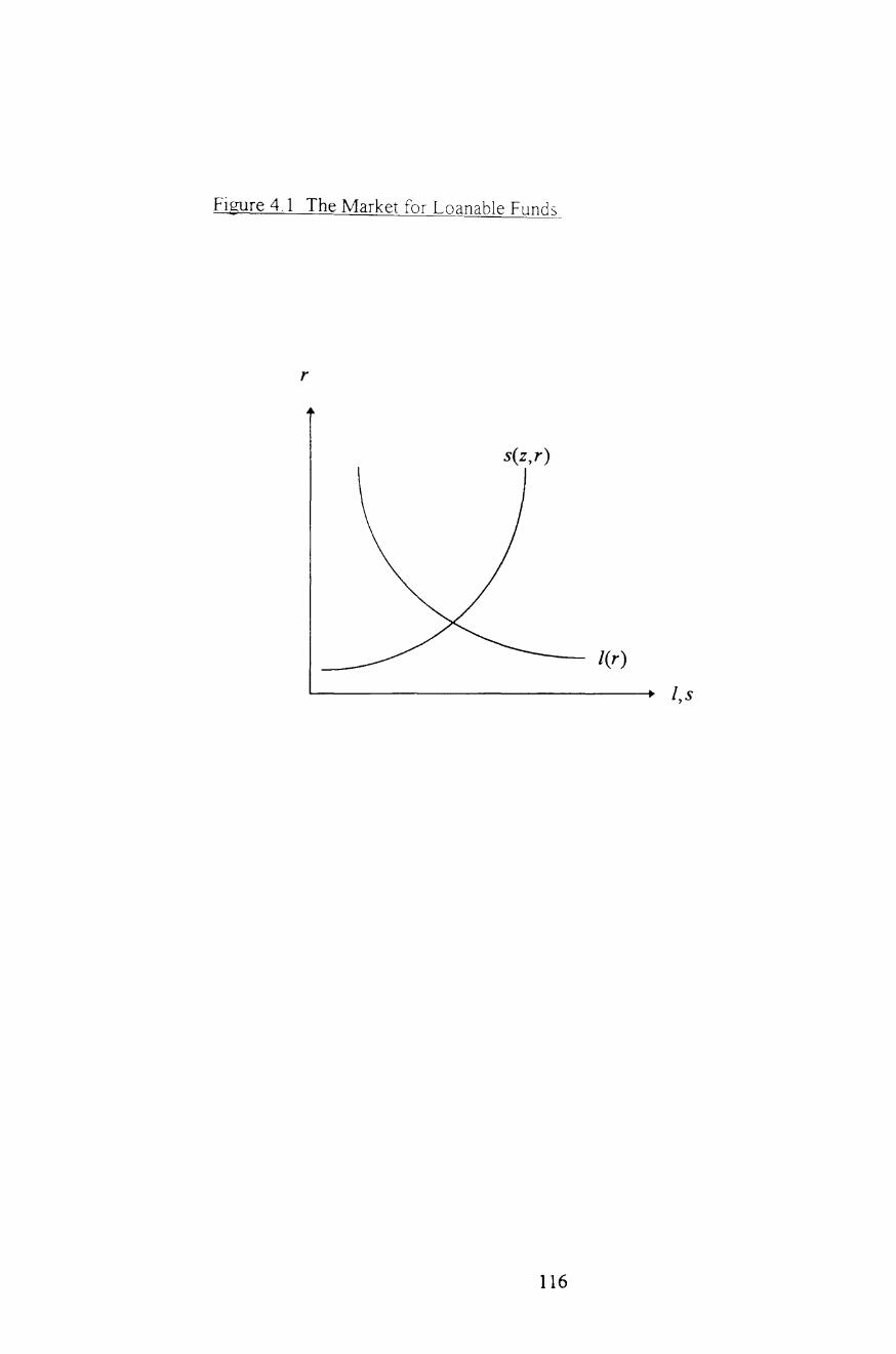
Figure 4.1 The Market for Loanable Funds
r
s(z,r)
I(r)
I, s
116

We are interested in what the predictions are of this model concerning the link
between inequality and the volume of intermediatioI\ since this is the relationship
we want to base our test of the model on. We want to separate out the effect from
changes in the level of national income per capita from the analysis since this
variable previously has been shown to affect the volume of intermediation. To do so
we can model an increase in inequality as a mean preserving spread on the
distribution of entrepreneurial wealth. A mean preserving spread places more
weight on the tails of the distribution without changing the mean. Thus a mean
preserving spread on a wealth distribution increases the variance of the distribution.
Formally a mean preserving spread can be defined in the following way 11 :
For two distributions GU (w) and G~ (w) with support [Wi, w h l G~ (li') is
said to be a mean preserving spread on GU (w) (or equivalently GU (w) second
order stochastically dominates G~ (w)) if the following conditions are satisfied:
wh
i) f [Gu (w) - G~ (w)] dw = 0 (Identical means)12 and, wi
w· ii) f[G~(w)-GU(w)]dw~O Wi sw# sw h
wi
This is the definition of a mean preserving spread given by Rothschild and
Stiglitz(1970,1971). We will also assume that the two distributions we study satisfy
the single crossing property, namely
iii) GP (w) - GU (w) s 0 (~ 0) when w ~ (spy
11 See Sargent(l987) pp. 64-65. and Mas-CoIeIL Whinston and Green(1995) pp.I97-I99. I: See Sargent(l987) p.58 for the derivation of the mean of a non-negati\"e random \"ariable.
117

Figure 4.2 Mean Preserving Spread SatisfYing the Single Crossing Property!:3
1 II--------------------~~------
~----______ +_------------l \iv" ~ w h1
Figure 4.3 Mean Preserving Spread Violating the Single Crossing Propert\
A,1foO. ,.\ \ A.~ g
~\ (A~(.l ~ /~~(~d»)
13 Sources: ~2.: Sargent( 1987). ~.3.: Mas-Colcl!. \\'hlllston and Grcen(l995)
118

This is a type of mean preserving spread illustrated in figure 4.2. A mean
preserving spread that does not satisfy condition (iii) is illustrated in figure 4.3. This
assumption greatly simplifies the subsequent analysis. Given that we in our data
work study changes only at top and bottom quintile of the wealth distribution this is
also a sensible assumption.
Given the above definition we can describe what happens to the loan demand
curve when there is a mean preserving spread of the distribution of entrepreneurial
wealth.
Loan demand is given by,
wh
(9) I(r) = f [k} (r) - w}iG(w) w*(r)
This can also be written
w*(r)
I(r) = 1- f [k} (r) - w}iG(w) wi
U sing the integration by parts rule (f vdu = uv - f udv) on the above
expression, we get
w*
I(r) = 1- [k} (r) - w]G(w)I:; - f G(w)dw wi
w*
(12) = 1- [k} (r) - w *]G(w*) - f G(w)dw wi
We can use (12) to describe the effects of a mean preserving spread on the
loan demand schedule holding the interest rate constant. Index the loan demand
119

function by the spread ranking of the distribution so that la (r) is the loan demand
function associated with Ga (w), and I~ (r) is associated with G~ (w) . Then.,
".* (13) r (r) -/~ (r) = [Ga (w*) - G~ (w*) ~w * -k1 (r))+ f [G~ (w) - Ga (w) lru.
"/
We can use the definition of a mean preserving spread satisfying the single
crossing property to sign la (r) -/~ (r) . By condition (ii) f [G~ (11') - Ga (w)}tw is wI
always positive. The sign of [Ga (w*) - G~ (w*) Xw * -k1 (f)) is ambiguous.
(w * -k] (r)) is always negative, but as can be seen from condition (iii) the sign of
[Ga
(w*) - G~ (w*)] changes as w * changes relative to w. If w* ~ w then
[Ga(w*)-G~(w*)];:::O. This implies that [Ga(w*)- G~(w*)Xw*-k1(r))is
negative and hence la (r) -/~ (f) can be negative. If on the other hand w* ~ w ,
then [G a (w*) - G~ (w*) Xw * -k1 (f)) is positive and thus la (f) -l~ (f) is
positive.
This ambiguity arises because a mean preserving spread has two effects. It
affects the average wealth of agents with access to the intermediated sector, and it
affects the total number of these agents. A mean preserving spread will always
increase the average wealth of the agents with access to intermediation, since only
the wealth levels above the cut off point w * affects this average. Since we are
investigating the effects of a mean preserving spread holding the interest rate
constant, the size of the optimal investment project does not change in our analysis,
therefore the aVerage amount each entrepreneur needs to borrow is reduced by the
average wealth effect of a mean preserving spread. This effect thus suggests that
increased inequality should reduce the amount of intermediation. However this need
not be the case, because the mean preserving spread also changes the number of
120

Figure 44a Mean preserving Spread in a Relativeh' Poor Economy
Figure 44b Mean Preserving Spread in a Relatively Rich Economy
~'~J r I I I , I I I
i i
I i
121

entrepreneurs with access to intermediation. When one performs a mean preserving
spread one shifts mass from the centre of the distribution towards the tails. Assume
that this is done in a way so that equal probability mass is shifted to the top and
bottom tails of the distribution. If the cut off point for borrowing lies at a relati\·e
high point in the support, more mass is shifted above the cut off point by a mean
preserving spread, and thus there will be more borrowers in this economy, this is
illustrated in figure 4. 4a. If on the other hand the cut off point for borrowing lies at
a relatively low point in the support, then more mass is shifted below the cut off
point, and there will be fewer borrowers in the economy, this is illustrated in figure
4.4b.
Since w is a given point in the support, one can say that the dependence of
the sign of fa. (f) -f~ (f) on the location of w * implies a conditionality on the
level of national income of the relationship between inequality and the volume of
financial intermediation. An economy with a high w * is on average poorer than an
economy with a low w * , thus the result above can be interpreted as saying that for
a poor economy increased inequality will increase the volume of financial
intermediation if the numbers effect dominates the average effect, while for a rich
economy more inequality will unambiguously reduce the volume of intermediation
since both effects work in the same direction.
To sum up: In a poor economy increased inequality shifts the loan demand
schedule (figure 4.1) to the right for a given interest rate. In a rich economy the
curve shifts to the left.
To illustrate this point we have performed simulations of the effects of a mean
preserving spread on the volume of loans demanded. The simulation is performed
using a normal distribution 14. We hold the mean constant and look at the effects of
changing the variance of the distribution. The simulated economy has a population
14 This simulation is strictly speaking not a true representation of our problem since the support of
a nonnal distribution is (-00,00), howeyer as long as we make sure that the k \ we choose is
larger than any actual realisation. we can still use a simulation based on a nonnal to illustrate our point.
122

of size 100, kl equals 30 and the average per capita income is 15. An increase in
the variance of income is equivalent to an increase in the degree of inequality in the
economy. As figure 4.5 illustrates: For values of w* above the mean (v.;>15)
increased inequality increases the volume of loans demanded. That is, a poor
economy with a more egalitarian income distribution will have less satisfied loan
demand than an economy with the same mean income, but a higher degree of
inequality. The reverse is true for economies where w* is below the mean (w<15)
i. e. relatively rich economies. These results are identical to the predictions of the
theoretical model above.
So given the upwards sloping savings supply schedule the equilibrium effects
of a mean preserving spread of the wealth distribution depends on the level of per
capita income in the economy. For a poor economy, a mean preserving spread will
shift the I curve in figure 4.1 to the right, thus increasing the equilibrium volume of
financial intermediation, while for a richer economy it will shift it to the left,
reducing the volume of financial intermediation. We summarise the hypothesis that
can be derived from the above analysis concerning the transmission mechanism
between inequality and financial development.
Hypothesis: The relationship between inequality and financial development is
conditional on the level of per capita national income in the following way: for low
income countries higher inequality increases the amount of intermediation; for high
income countries it decreases the amount of intermediation.

Figure 4.5 Simulations ofInequaEty and Intermediation.
2500,00 · : : .
: .. : :: .
2000,00 . : : :
· .. :: : . . : .: ..
· . c 1500,00 . . o :.:.
:;:; ca =g E ~ CI) -c 1000,00
· : .,':.
· : : : .
: : : . . . . . : . .. . : . . . . .
. . : . . · .
. : : :
· : . .
.... ::.
· .:
.. . .
: . : : .
:: : .:::: . . .::\:::: .:-:: ) .. '::: , , . . .. • ,. ,li .' ,'!'jim" : : :: .. . .: :: . : : : : j::::l::;::~:{ . :r}::: . :::::.;;::i : : : ," ..
.::: :: ::.: :' ~ . . . .
... ". : ;: ::.
..: ',. ,'. . ..
.. : . : ": ..
500,00
0,00
o
: : : . · ...
,,: : : .. ' .
· .. · ...
.. :
. . , ..
": :. ' . . . . . · ::>;;; .: .,,:
2
: : .: . . : ; ~ : '. : ::
. . . : .
: : : :: ::': :::I' .. :..:::t . : ::~ . ];:1:::::::::::::: 1 : :0 . :::j::: :::;:=:: :::.::}: : :': , .::':~:{::::?:::::::
4 6 8 10
Inequality
<> W>6
oW>10
A W>13
xW>15
xW>17
o W>20
- Inequality increases from 0 (lowest) to 10 (highest). Each step is equivalent to a mean preserving
spread on the wealth distribution.
- Each set of points traces the change in intermediation as inequality changes for an economy with
a given cut-off level of wealth.
124

4.3 Empirical evidence.
4.3.1 Data
To examine the links between financial development and income inequality,
we look at cross-sectional evidence for 50 countries15 . The data on income
inequality comes from the Deininger and Squire (1996) data set. This data set is a
compilation of the findings of a large number of inequality studies and was put
together to facilitate cross-sectional analysis. Only observations based on household
surveys, a comprehensive coverage of the population and a comprehensive
coverage of income sources has been included. The data set is the largest available
and contains 682 "high quality" observations covering 108 countries. There are still
substantial problems with the data set. The most pertinent problems related to the
cross-country analysis are firstly that the data set varies in its coverage of different
countries, therefore we cannot be sure to have observations for the same year for all
the countries in our sample. We have chosen yearly observations as close as
possible to each other. Our data set contains countries with observations in the
1986-1994 range. The second problem is that the definitions used in different
studies are not identical. These differences arise from: (i) Whether the recipient unit
is the household or the individual; (ii) Whether income or expenditure is used for
measurement; :(iii) Whether income is measured gross or ne~ of taxes; The first two
differences are the most serious since the difference between gross income and net
of tax income is most significant for inequality studies in economies where the tax
system is used for re-distributive purposes. This is mostly the case in highly
developed economies that are not part of our sample. Deininger and Squire have
analysed the importance of the differences in definition of the recipient unit and the
difference between income and expenditure studies. They find that only the income
expenditure difference has significant effect on the data analysis. In spite of these
problems we have chosen to conduct the empirical investigation. The Deininger and
15 The constraint on the size of the sample comes from the inequalit) data set. Financial data is available for a large group of countries through the IFS and standard cross-sectional controls are available for more than 100 countries. The King and Levine data set for the investigation on the link between financial development and growth thus consists of 119 countries.
125

Squire data base is the best available and can help shed some light on an important
question. Furthennore we have where possible addressed the problems of data
definition. The conclusions of our empirical investigation should however be read
with the above problems in mind.
The Deininger and Squire data set contains two types of measures of
inequality; Gini coefficients and cumulative quintile shares of income. The data set
has the widest coverage for Gini coefficients, but this measure is not directly related
to our model since redistribution of income anywhere in the income distribution
affects the Gini coefficient, while we are interested in agents crossing a cut off
point. Therefore we rely on quintile income shares to measure inequality. We use
the ratio of the income share of the top 20 percent of the population to the income
share of the bottom 20 percent of the population. We call this variable Inequality
This is a relative measure of inequality and gives us infonnation of how poor the
least well off members of the society are relative to the richest members. An
increase in Inequality is equivalent to introducing a mean preserving spread on the
wealth distribution in our model. Alternatively one can think of capturing the
fraction of agents below the cut off point. This is done through the variable Poverty
which measures the income share of the lowest quintile of the population. In using
income shares for the entire population to test the hypothesis on the link between
inequality and financial development, we are implicitly assuming that this variable is
a good instrument for the key variable in our theoretical model which is the wealth
of agents in the entrepreneurial sector. It is not unrealistic to assume that income
and wealth are highly correlated especially since some income is flow income from
the agent's stock of wealth. Further, if the entrepreneurial sector covers a
significant share of the total economy one would expect the distribution covering
the economy to be a good proxy for the distribution of the entrepreneurial sector.
However the fact that a one to one mapping does not exist between the variable in
our theoretical model and the instrument, induces us to urge further caution when
interpreting the empirical results.
126

To measure the degree of financial development, we use the ratio of financial
sector claims on non-bank private sector16 to GDP. We call this variable
Intermediation. This measure of financial depth is also used by Townsend(l983)
and King and Levine (l993a,b).
Our model suggests that the sign of the effect of changes in inequality on the
level of financial development is conditional on the level of economic development
in the economy (measured as per capita national income). For low income countries
there should be a positive correlation between inequality and financial depth, for
high income countries the correlation should be negative. We use GDP per capita
reported in US$ as a measure of the level of economic development 17. We call this
variable Income.
4.3.2 Preliminary Investigation
Figure 4.6 shows a scatter plot of pairs of Intermediation and Inequality for
the entire sample. As is evident from the plot there is no obvious linear relationship
between the variables. The correlation matrix in table 4.1 shows a small negative
relation between the two variables. Likewise there is no obvious relationship
between Poverty and Intermediation as can be seen from figure 4.7. The correlation
matrix in table 4.2 shows a small positive relation. Figure 4.8 shows that after
conditioning on Income there is still no obvious relationship between
Intermediation and Inequality.
4.3.3 Regressions
Our model pays particular attention to the demand side in the financial sector.
We have ignored potentially interesting features on the loan supply side. In the
empirical section we compensate for this by introducing various controls which
might affect the supply of funds. Political stability is important for savers' reliance
16 Claims on non-bank private sector is the IFS 32.d. series. GDP is the IFS series (99.b). 17 Population is IFS series 99.2, We use annual averages of the exchange rate of the national currency to USS to convert our GDP measure into USS (IFS country exchange rate series ... af).
127

Figure 4.6 Plot of Intermediation and Inequality
40~----------------------~ lmJwlity
30
20-+
10 +
+ +
+
+
++
.t
+
+
+.{+ + +
+
*
+ +# + ++ ++ +:j: ++
0 0.0 0.2
+
Table 4.1 Correlation Matrix
Inegual!!y Inequality 1.0 Intermediation -0.026
+
+
+
+
+ + + + + + + + + +
0.4 0.6 0.8 1.0
lrIterrmliatim
Intermediation -0.026 1.0
128

Figure 4.7 Plot of Intennediation and Poverty
0.10 + +
Poverty + + +
+ + +
0.08 +
+ + +
+ + + + + + + + 0.06 ++
+ + + + +
+++ + +
0.04 + + -++- + +
+ + +++ +
+ +
0.02 *" + +
o. 00 -+----r--------.----.------.---~ 0.0 0.2 0.4 0.6 0.8 1.0
Intennediation
Table 4.2 Correlation Matrix
Poverty Intennediation Poverty 1.0 0.057 Intennediation 0.057 1.0
129

Figure 4.8 Plot of Intennediation and Inequality after Conditioning on Income
Intennediation 0.6-~----------------------------~
0.4- + +
+ ++ +
0.2-+ +
+
~ + :t: t + ++ 0.0- + + -: +
...... + + + + + f + + + + + +
+ + ++ + + + + -0.2- +
+
-0.4 -IL------.-------r----,---------r
o 1 20 30 10 o
Inequality
130

on the financial sector. The governments share in GDP might play a role too, the
infrastructure of the economy such as the size of the agricultural sector and
population density could be important, and the openness of the economy might
affect the interest elasticity of savings supplies.
To test our hypothesis we ran the following OLS regression.
(14)
Intermediation = Po + p/ncome + P2Income x Inequality
+ P 3 Income 2 x Inequality + ~ 4 Inequality
+ psIncome2 + Controls
The Income term and interaction terms between Income and Inequality are
directly derived from our theoretical analysis. These terms contain the non-linear
relationship between Intermediation and Inequality conditional on the level of
Income. This can be seen when we differentiate the expression with respect to
Inequality. We get;
a Intermediation A 1 A 1 ., A (15) =""21ncome+""31ncome- +""4 a Inequality
We expect to find a positive relationship between Intermediation and
Inequality for low income countries, while we expect to find a negative relationship
for high income countries. Equation (15) describes a second order polynomial in
Income. The sign switches will take place at the income levels which are the zeros
of this polynomial and these can be found using the standard formula
As is normal procedure in regressions with interaction terms we include all
the terms used in interaction separately, i.e. Income, Income2 and Inequality even
though our model does not hold any predictions on the coefficients of these
131

variables. We add a number of controls to the regression. Open defined as the sum
of exports and imports as a proportion of nominal GDP, measures the degree of
openness of the economy. This variable is taken from the Summers and
Heston(l991) data set. Govt is defined as the real government share of GD P
expressed in percent and is also taken from Summers and Heston(1991). Ch' and
Pol are the Gastil indicies of civil and political liberties. The Civil Liberties index
runs from 1 which is a ranking given to the most free countries to 7 which is Qiven ~
to the least free. The ranking is done by a research team at Freedom House18 . Rev
measures the average number of revolutions and coups per year and is taken from
King and Levine(l993a). Latin and Africa are dummy variables controlling for
countries in Latin America and sub-Saharan Africa respectively. We use the same
categories as King and Levine(1993). Popden is populatiGn density measured as
total population divided by area in square kilometres. Agriculture is the share of the
agricultural sector in value added as a share of GDP at market prices. Both these
are calculated from the World Bank 1995 data set available on-line at the LSE.
Table 4.3 contains the coefficient estimates of regression (14). ~3 and fu are
both significant at the 5-percent level while ~4 is only significant at the 20 percent
level. We calculate the roots of the above polynomial on the basis of these
coefficients; they are (z} ,Z2) = (613, 3835). These roots are calculated as a non
linear combination of our OLS coefficient estimates. We use the Wald test to test
the significance of these roots; z} is greater than zero with probability 0.8, and
(z}, Z2) are different from each other with probability 0.93. The roots imply that in
countries with a GDP per capita between US$ 613 and 3835 there is a positive
relationship between Inequality and Intermediation while the relationship is
negative for income levels above US$ 3835 and below US$ 613. The positive effect
18 See J.E.Ryan (1994) litt: The Comparative Sun'ey of Freedom 1993-1994 Survey Methodology pp.671-695 in: Freedom in the World: The Annual Survey of Political Rights And Ci\11 Liberties Freedom House. New York. Political rights enable people to participate freely in the political process (the checklist on which the ranking is based includes amongst other things: elections. parties. opposition rights access to office. political decentralisation.) Ci\il liberties are the freedoms to develop views, institutions and personal autonomy apart from the state (the checklist includes: free media, freedom of assembly. equality under the law. absence of political terror. free business organisation. free religion. personal freedoms. freedom from government corruption.)
132

is largest at the top point of the polynomial located at -~ which is equal to USS 2~
2224. Notably both sign switches take place at income levels contained in our
sample. The first root is the income level where the effect of increased inequality on
intermediation goes from negative to positive and the second root is the level where
the switch is from positive to negative. The data suggests that the model predicting
a sign switch when one goes from poor to rich countries is only partially right. For
very poor countries the effect of increased inequality on intermediation is negative,
which is contrary to the predictions of the theoretical model. A calculation using
our regression coefficient values suggest that Intermediation (measured as claims
on non-bank private sector as a percentage of GDP) in a country with a GDP per
capita ofUS$ 1000 will increase by 0.3 percent if Inequality is increased by 1 (i.e. if
the ratio of the income share of the top quintile to the bottom quintile goes up by
1). In our sample Inequality takes on values between 4.06 (in Bangladesh with per
capita GDP ofUS$ of 191) and 32.11 (in South Africa with GDP per capita ofUS$
of 2960), so a change of Inequality by 1 is realistic. However the conclusion on the
impact on I~termediation rests on a cross-country regression and is therefore
merely suggestive. Taking this analysis one step further one is tempted to use the
results from King and Levine ( 1993 a) (see specifically their table IX on p. 73 3)
which suggest that a 0.3 percent change in Intermediation19 will increase the
average growth rate of the economy in the subsequent decade by less than 0.01
percent. Thus the implied effects of changes in inequality on real GDP growth are
quantitatively small. If these results are to be taken at face value, changing
inequality would therefore not seem to be the policy variable one should focus on if
one wishes to increase real GDP growth in an economy.
19 Our variable Intermediation is equivalent to King and Levine' s Pri\~v 1. According to King and Le\ine table IX a change in Pri\y1 by 1 percent will increase the average annual grO\\th rate of the economy in the subsequent decade by 0.037 percent.
133
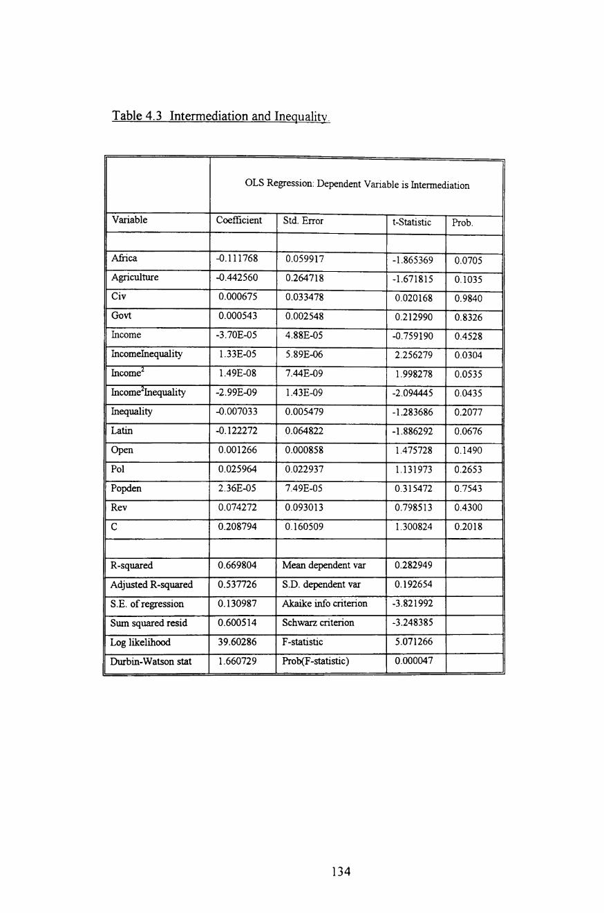
Table 4.3 Intermediation and Inequality.
OLS Regression: Dependent Variable is InteITIlediation
Variable Coefficient Std. Error t-Statistic Prob.
Afiica -0.111768 0.059917 -1.865369 0.0705
Agriculture -0.442560 0.264718 -1.671815 0.1035
Civ 0.000675 0.033478 0.020168 0.9840
Govt 0.000543 0.002548 0.212990 0.8326
Income -3.70E-05 4.88E-05 -0.759190 0.4528
IncomeInequality 1.33E-05 5.89E-06 2.256279 0.0304
Income2 1.49E-08 7.44E-09 1.998278 0.0535
Income2Inequality -2. 99E-09 1.43E-09 -2.094445 0.0435
Inequality -0.007033 0.005479 -1.283686 0.2077
Latin -0.122272 0.064822 -1.886292 0.0676
Open 0.001266 0.000858 1.475728 0.1490
Pol 0.025964 0.022937 1.131973 0.2653
Popden 2.36E-05 7.49E-05 0.315472 0.7543
Rev 0.074272 0.093013 0.798513 0.4300
C 0.208794 0.160509 1.300824 0.2018
R-squared 0.669804 Mean dependent var 0.282949
Adjusted R-squared 0.537726 S.D. dependent var 0.192654
S.E. of regression 0.130987 Akaike info criterion -3.821992
Sum squared resid 0.600514 Schwarz criterion -3.248385
Log likelihood 39.60286 F -statistic 5.071266
Durbin-Watson stat 1.660729 Prob(F -statistic) 0.000047
134

Of the interaction terms neither Inequality nor Income per se have significant
coefficients while this is the case for Income2. This suggest that there is a non-linear
relationship between Intermediation and Income. Of the controls only Agriculture
and the two regional dummies Latin and Africa are significant at the 10-percent
level. Agriculture has a negative coefficient which indicates a negati\'e relationship
between the share of agriculture in the economy and the degree of intermediation.
This seems sensible as one would expect agricultural economies to have a less
developed infrastructure overall than an economy with large industrial and service
sectors. Open, though only significant at the 85 percent level, has a positive
coefficient which is in accordance with what we expect given our model. A more
open economy is likely to have a higher interest elasticity C'f savings supply~ the s
curve in figure 4.1 is therefore flatter and when loan demand goes up, equilibrium
intermediation goes up more than in a closed economy. The negative coefficients on
the two regional dummies suggest that countries located in Latin America or Sub
Saharan Africa have smaller financial sectors than other countries. This result is in
line with other studies which also find negative effects from a location in these two
areas.
Govt, Civ and Pol also have positive coefficients but neither are significant.
Rev surprisingly has a positive coefficient, even though one would expect agents in
politically unstable countries to save outside the formal financial sector which is an
easy target for a dictator in need of funding. However the coefficient is not
significant so we should not pay too much attention to this result. The structural
control Popd~n is also non significant. There are no obvio"J'J ~utliers as can be seen
in figure 4.9 which plots the regression residuals. In table 4.4 we report the result of
regression (14) after dropping the insignificant controls. This does not change the
prevIOUS results significantly, the relationship between Inequality and
Intermediation now takes on positive values at a per capita GDP between US$ 548
and 4418 with a peak at 2483 . For these coefficient estimates the Wald test shows
that ZI is greater than zero with probability 0.85, and (ZI' =:) are different from
each other with probability 0.98.
135

Figure 4.9 Residuals From Inequalitv Regression (Table 4.3)
0.4
0.2
-0.2
r--------------------.-1.0
0.8
0.6
5 10 15 20 25 30 35 40 45 50
1-- Residual ------- Actual ---- Fitted I
136
0.4
0.2
0.0

Table 44 Intermediation and Inequalitv (excluding some controls)
OLS Regression: Dependent Variable is Intermediation
Variable Coefficient Std. Error t-Statistic Prob.
Afiica -0.125966 0.053690 -2.346158 0.0240
Agriculture -0.223693 0.215414 -1.038435 0.3053
Income -5.65E-05 4.43E-05 -1.274992 0.2097
IncomeInequality 1.44E-05 5. 36E-06 2.681182 0.0106
Income2 1.53E-08 6. 84E-09 2.241482 0.0306
Income2Inequality -2.90E-09 l.27E-09 -2.290338 0.0274
Inequality -0.007017 0.005200 -l.349295 0.1848
Latin -0.162801 0.055526 -2.931984 0.0055
Open 0.001605 0.000564 2.844221 0.0070
C 0.287522 0.097120 2.960477 0.0051
R-squared 0.637612 Mean dependent var 0.282949
Adjusted R-squared 0.556075 S.D. dependent var 0.192654
S.E. of regression 0.128361 Akaike info criterion -3.928963
Swn squared resid 0.659060 Schwarz criterion -3.546558
Log likelihood 37.27715 F -statistic 7.819895
Durbin-Watson stat 1.816469 Prob(F -statistic) 0.000002
137

We also tried running regression (14) substituting the Inequality variable \\lith
Poverty. The regression coefficients are reported in table 4.5. The results are ver\"
different from the regression using Inequality: even though the roots are estimated
to be located at VS$ 433 and 4393 and thus are similar to the previous findings, the
sign of the coefficient on Income2Poverty is positive implying that the estimated
polynomial has a V-shape rather than an inverted V-shape. The sign switches are
therefore the opposite of what was the case for the Inequality regression. Increases
in Poverty increases the amount of Intermediation for poor countries with GDP per
capita below VS$ 433 and for rich countries with GDP per capita above US$ 4393.
F or countries with per capita income between these two values increased Poverty
reduces Intermediation. Z1 is greater than zero with probability 0.5, and (Z1' =2)
are different from each other with probability 0.77. The signs and significance of the
controls are very similar to the earlier results using Inequality. However Poverty is
only significant at the 40 percent level making the conclusions here weaker than
when using the Inequality variable. Figure 4. 10 plots the residuals from this
regression, again there are no obvious outliers.
Table 4.6 reports the Poverty regression excluding insignificant controls. In
this regression the Poverty-Intermediation relationship is negative for income levels
between US$ 509 and 4567. In this regression Z1 is greater than zero with
probability 0.6 and (Z1 ,Z2) are different from each other with probability 0.77.
The sign switches found using the Poverty are completely contrary to the
predictions of our theoretical model. However the hypothesis we derived in the
theoretical section is based on changes both at the top and at the bottom of the
income distribution, this is captured better by our Inequality variable than by our
Poverty variable, which only contains information about income of the bottom
quintile.
138

Table 4.5 Intermediation and Poverty.
OLS Regression: Dependent Variable is Intermediation
Variable Coefficient Std. Error t-Statistic Prob.
Africa -0.117769 0.065176 -1.806931 0.0794
Agriculture -0.454761 0.269512 -1.687351 0.1004
Civ -0.003190 0.033866 -0.094191 0.9255
Govt 0.001139 0.002538 0.448960 0.6562
Income 0.000251 0.000133 1.882797 0.0681
Income2 -4.45E-08 1.98E-08 -2.253734 0.0306
IncomePoverty -0.002698 0.001838 -1.467538 0.1512
Income2Poverty 5.59E-07 2.60E-07 2.147786 0.0387
Latin -0.120947 0.072284 -1.673223 0.1032
Open 0.001137 0.000863 1.317403 0.1963
Pol 0.030787 0.023084 1.333675 0.1909
Popden 3.38E-05 7.12£-05 0.475201 0.6376
Poverty 1.065360 1.861116 0.572431 0.5707
Rev 0.081135 0.093347 0.869174 0.3907
C 0.068312 0.234200 0.291684 0.7723
R-squared 0.672753 Mean dependent var 0.282949
Adjusted R-squared 0.541854 S.D. dependent var 0.192654
S.E. of regression 0.130401 Akaike info criterion -3.830962
Sum squared resid 0.595152 Schwarz criterion -3.257355
Log likelihood 39.82712 F -statistic 5.139487
Durbin-Watson stat 1.712743 Prob(F -statistic) 0.000041
139

Figure 4.10 Residuals From Poverty Regression (Table 4.5)
0.3
0.2
0.1
0.0
-0.1
-0.2
-0.3
.-------------------------------------------~1.0
5 10 15 20
Residual
25 30 35 40
------- Actual ----. Fitted
140
45 50
0.8
0.6
0.4
0.2
0.0

Table 4.6 Intermediation and Poverty (excluding some controls).
OLS Regression: Dependent Variable is Intermediation
Variable Coefficient Std. Error t-Statistic Prob.
Africa -0.124087 0.058865 -2.107988 0.0415
Agriculture -0.402287 0.241940 -1.662756 0.1044
Income 0.000243 0.000116 2.090351 0.0432
Income2 4.l4E-08 1.77E-08 -2.331044 0.0250
IncomePoverty -0.002660 0.001653 -1.609317 0.1156
Income2Poverty 5.24E-07 2.36E-07 2.217275 0.0325
Latin -0.120023 0.066793 -1.796952 0.0801
Open 0.001333 0.000544 2.451486 0.0188
Pol 0.027543 0.013901 1.981422 0.0546
Poverty l.218290 1.640385 0.742686 0.4621
C 0.087741 0.151982 0.577310 0.5670
R-squared 0.661369 Mean dependent var 0.282949
Adjusted R-squared 0.574540 S.D. dependent var 0.192654
S.E. of regression 0.125663 Akaike info criterion -3.956766
Sum squared resid 0.615855 Schwarz criterion -3.536121
Log likelihood 38.97223 F -statistic 7.616958
Durbin-Watson stat 1.744376 Prob(F -statistic) 0.000001
141

As mentioned earlier the Deininger and Squire data set contains observations
using different data definitions of income levels; some observations are income
based and some are expenditure based. Some observations· are of household units
some are of individuals. To control for the income/expenditure difference we split
the sample into two sub-samples; one contains the income based observations and
one contains the expenditure based observations. We then run regression (16)
estimating (Z1' Z2) separately in the two sub-samples. Next we control for the
difference between household based and individual based observations in the same
way in regression (17).
Intermediation = ~ 0
+~ 1 D1 Income + ~ 2 D1 Income X Inequality + ~ 3D1 Income 2 X Inequality
(16) +~4DJnequality + ~sDJncome2
+~ 6D2Income + ~ 7D2Income x Inequality + ~ sD2Income 2 x Inequality
+~9D2Inequality + ~IOD2Income2 + Controls
Intermediation = ~ 0
+~ I D3Income + ~ 2D3Income x Inequality + ~ 3D3 Income 2 X Inequality
(17) +~ 4D3Inequality + ~ SD3Income2
+~ 6D4Income + ~ 7D4Income x Inequality + ~ sD4Income2 x Inequality
+~ 9D4Inequality + ~ IOD4Income2 + Controls
In regressIOn (16) we pay attention to the fact that some countries (17
countries) in our sample use income based measures while others (33 countries) use
expenditure based measures. We allow the sign switch point to be estimated
separately for these different definitions by introducing two dummy variables. D)
takes the value 1 when the data is income based and zero otheIWise. D.. takes the
142

value 1 when data is expenditure based and zero otherwise. The sign switch points
for the income based data are
and for the expenditure based data the switch points are
Table 4.7 reports the regression coefficients for regression (16). While both
types of data definitions still estimate a positive sign switch point, the point varies
significantly. For the expenditure measure the sign is positive for income levels
between US$ -3006 and 327 while it is positive for levels between US$ 152 and
6496 for the income based measure. For the expenditure based observations Z I is
different from zero with probability 0.63 and (Zl' Z2) different from each other with
probability 0.66. For the income based observations ZI is different from zero with
probability 0.1 and (ZI ,Z2) are different from each other with probability 0.69. The
Zl estimated from expenditure based data is more significanc than the ZI estimated
from income based data. This is not too surprising given that the share of
expenditure based observations in the sample is largest (33 against income based
data 17). The two ZI 's estimated using the two sub-samples are different from each
143

Table 4.7 Intermediation and Inequality (Income and Expenditure Data)
OLS Regression: Dependent Variable is Intermediation
Variable Coefficient Std. Error t-Statistic Prob.
Africa -0.129996 0.062589 -2.076964 0.0465
Agriculture -0.375299 0.277041 -1.354671 0.1856
Civ -0.016372 0.032658 -0.501310 0.6198
D2Income 0.000265 0.000136 1.956748 0.0597
D2IncomeInequality -1.38E-05 1.66E-05 -0.832392 0.4118
D2Income2 5.41E-09 1.32E-08 0.410800 0.6841
D~come2Inequality -5.15E-09 2.74E-09 -1.88lO44 0.0697
D2Inequality 0.005054 0.007378 0.685080 0.4986
Govt 0.000322 0.002662 0.120864 0.9046
D1Income -4. 78E-06 5.76E-05 -0.082857 0.9345
DIIncomeInequality 8. 11E-06 9.71E-06 0.835613 0.4100
D1Income2 5.42E-09 1.16E-08 0.466438 0.6443
D1Income2Inequality -1.22E-09 2.43E-09 -0.501467 0.6197
DIInequality -0.001204 0.009148 -0.131646 0.8961
Latin -0.130277 0.063053 -2.066146 0.0475
Open 0.001200 0.000819 1.465506 0.1532
Pol 0.020604 0.022699 0.907699 0.3713
Popden -1. 12E-05 8.02E-05 -0.140110 0.8895
Rev 0.094094 0.088715 1.060630 0.2973
C 0.181658 0.164822 1.102145 0.2792
R-squared 0.747809 Mean dependent var 0.282949
Adjusted R-squared 0.588087 S.D. dependent var 0.192654
S.E. of regression 0.123646 Akaike info criterion -3.891489
Sum squared resid 0.458651 Schwarz criterion -3.126680
Log likelihood 46.34030 F -statistic 4.681961
Durbin-Watson stat 1.437849 Prob(F -statistic) 0.000088
144

Table 4.8 Intermediation and Inequality (Household and Indi\idual Data)
OLS Regression: Dependent Variable is Intermediation
Variable Coefficient Std. Error t-Statistic Prob.
Africa -0.147815 0.065471 -2.257697 0.0314
Agriculture -0.374445 0.301189 -1.243225 0.2234
Civ -0.009769 0.036562 -0.267184 0.7912
Govt 0.000745 0.002633 0.282912 0.7792
DJlncomeInequality 2.04E-05 1.12E-05 1.815683 0.0794
DJlncome -7.83E-05 6.36E-05 -1.231575 0.2277
DJlncome2 2.09E-08 8.75E-09 2.388728 0.0234
DJlncome2Inequality -3.92E-09 2.26E-09 -1.735104 0.0930
DJlnequality -0.011551 0.016039 -0.720176 0.4770
Latin -0.132549 0.079934 -1.658240 0.1077
Open 0.001346 0.000885 1.521901 0.1385
DJncomeInequality 6. 82E-06 1.81E-05 0.376563 0.7091
DJncome 4.39E-05 0.000119 0.368497 0.7151
DJncome2 9.21E-09 3.46E-08 0.265983 0.7921
DJncome2Inequality -2.63E-09 6. 64E-09 -0.3963l3 0.6947
DJnequality -0.002320 0.008841 -0.262447 0.7948
Pol 0.027505 0.025936 1.060492 0.2974
Popden 3.04E-05 9.69E-05 0.313367 0.7562
Rev 0.082552 0.099794 0.827225 0.4146
C 0.185086 0.182280 1.015396 0.3180
R-squared 0.706298 Mean dependent var 0.282949
Adjusted R-squared 0.520287 S.D. dependent var 0.192654
S.E. of regression 0.133435 Akaike info criterion -3.739111
Sum squared resid 0.534145 Schwarz criterion -2.974302
Log likelihood 42.53086 F -statistic 3.797069
Durbin-Watson stat 1.657451 Prob(F -statistic) 0.000556
145

other with probability 0.62. The results highlight the fact that the exact location of
the income interval where the effect is positive is sensitive to data definitions used
in the regression.
Similarly regression (17) checks for the importance of differences between
Household based data (11 countries) and Individually based (39 countries). D3
takes the value 1 when the data is based on household units and zero otherwise. D-l
takes the value 1 when data is based on individual units and zero otherwise. Table
4.8 reports the coefficients of regression (17). The positive intervals lies between
income levels ofUS$ 646 and 4557 for household based data, while the interval is
between US$ 403 and 2190 for individually based data. The = I estimated using
household data is different from zero with probability 0.57 and (ZI ,=:) are different
from each other with probability 0.96. For the individual based sub-sample =1 is
different from zero with probability 0.21 and (ZI' Z2) are different from each other
with probability 0.28. The two =1 's estimated using the two sub-samples are
different from each other with probability 0.15. These findings again support the
conclusion that the non-linear relationship between measures of inequality in the
economy and the volume of intermediation exists and is conditional on the level of
per capita GDP. However the data suggests that there are two sign switches; one at
very low per capita income levels (around US$ 500) from negative to positive and
one (around US$ 4000) from positive to negative. The negative effect at very low
income levels is contrary to the predictions of our model. Also the exact location of
the income interval where the effect of inequality is positive varies across different
data definitions.
4.4 Conclusion
We set out to investigate the link between inequality and financial
development. Our investigation is based on a simple model linking these two
variables. The model relies on moral hazard in cutting off poorer agents from
intermediation. This is the same mechanism as is used other recent theoretical
146

models like Plketty(1997) and Aghion and Bolton (1997). We exogenously change
the degree of inequality by looking at a mean preserving spread to the wealth
distribution of entrepreneurs. The experiment suggests that one should expect to
find increased intermediation in poor economies as inequality is increased. In rich
economies one should expect to find that increased inequality reduces the amount
of intermediation. This difference arises because there are two effects on
intermediation of a mean preserving spread: first it increases the average wealth of
the entrepreneurs in the intermediated sector, which given the size of the optimal
investment project reduces the amount of borrowing in the economy. Second it
changes the number of people in the intermediated sector. In the poor economy it
increases the number of agents with access to intermediation, in the rich economy it
reduces this number.
In the poor economy the average effect and the numbers effect work in
opposite directions. Thus, if the numbers effect dominates the average effect, which
we assume it does, inequality increases intermediation. In the rich economy both
effects of a mean preserving spread work in the same direction: there will be fewer
agents with access to intermediation, and they will on average be richer. For a given
size of investment project in the economy, this reduces the amount of borrowing.
Thus increased inequality will unambiguously reduce intermediation in a rich
economy_
Next we go on to test the hypothesis that the relationship between inequality
and intermediation is conditional on the level of national income in a non-linear way
as described above. We use data from a new Wodd Bank data base covering a
cross-section of countries. The data set is the best available but there are still
definitional problems reducing the cross-country compatibility of the inequality
indicator. With this qualification in mind we find the predictions of the theoretical
model to be only partially borne out by the data. The analysis shows that increased
inequality increases intermediation in poor economies with income levels between
US$ 500 and US$ 4000. For income levels above US$ 4000 increased inequality
reduces intermediation as is predicted by our model. However in \'ery poor
147

economies (with GDP per capita below VSS 500) increased inequality reduces
intennediation. This is contrary to the predictions of our model. The exact location
of these switching points vary across different data definitions. However for both
the full sample regressions that use the Inequality variable the estimated roots (=:
around 500, Zj around 4000) are significant. The specific location of the interyal is
sensitive to the data definitions used as regression (16) and (17), using sub-samples
with more homogeneous observations, show. Thus the numbers above are merely
suggestive. The regressions run using the Poverty variable instead of Inequality find
similar roots. However the polynomial estimated has a V-shape rather than an
inverted V-shape as is the case for all the inequality regressions and indeed is
suggested by the theoretical model. Therefore the sign switches found using the
Poverty variable are the opposite of the ones described above. Poverty however
only contains infonnation about the bottom quintile of the income distribution and
is thus a poorer instrument than Inequality for capturing the effects of a mean
preserving spread. Therefore the Poverty findings do not falsify the theoretical
model given the findings of the Inequality regressions.
In the endogenous growth literature the models predict that increased
intennediation increases the real growth rate of the economy. This is the second
part of the channel from inequality to growth which we do not investigate in this
paper. However we can rely on King and Levine's (l993a) findings to get a grip on
the overall effect of inequality on real growth. When we do so, we find that the real
effect of increased inequality are very small for a model transmitting the effect
through the financial sector, so perhaps Lucas(l988) was right when he suggested
that financial variables had been overemphasised in the growth literature.
All in all we find support for the existence of the first part of the financial
transmissions mechanism linking inequality and growth, namely the inequality
intennediation link. But the sign effects derived from the data are only partially
consistent with the predictions of our theoretical model. Furthermore the scale of
the effects is very small suggesting that one should look for other channels linking
inequality and real growth before giving policy prescriptions on this issue.
148

Table 4.9 Data set
Income Intennediation Inequality Poverty Popden Agriculture 1 Algeria 1988 2279.68 0.60 6.85 0.0680 9.937 0.11 2 Banglades 1989 191.91 0.22 4.06 0.0950 737.042 0.37 3 Bolivia 1990 657.78 0.22 8.58 0.0562 6.032 0.32 4 Botswana 1986 1139.95 0.09 16.36 0.0360 1.915 0.05 5 Chile 1989 2174.63 0.47 17.03 0.0370 17.082 0.08 6 Colombia 1988 1296.70 0.14 15.11 0.0370 27.952 0.17 7 Costa Rica 1989 1789.60 0.16 12.68 0.0400 57.768 0.17 800M 1989 953.86 0.16 13.26 0.0420 142.760 0.18 9 Ecuador 1994 1480.02 0.23 9.82 0.0536 37.828 0.12
10 Egypt 1991 657.20 0.22 4.72 0.0871 54.187 0.17 11 Ghana 1989 360.26 0.06 6.33 0.0697 61.021 0.49 12 Greece 1988 6407.59 0.19 6.65 0.0619 76.636 0.14 13 Guatemala 1989 940.76 0.14 30.00 0.0210 82.062 0.26 14 Guinea 1991 238.46 0.14 28.57 0.0206 27.266 044
Bissau 15 Guyana 1993 568.94 0.17 7.48 0.0627 3.774 0.35 16 Honduras 1992 630.90 0.23 14.67 0.0384 46.171 0.17 17 India 1989 346.81 0.29 4.36 0.0910 251.788 0.28 18 Indonesia 1990 590.23 0.50 4.56 0.0920 93.509 0.21 19 Israel 1992 12636.80 0.58 5.25 0.0763 238.641 0.02 20 Jamaica 1989 1700.98 0.31 9.61 0.0510 216.105 0.07 21 Jordan 1991 944.45 0.64 7.37 0.0647 4l.071 0.07 22 Kenya 1992 309.36 0.23 18.24 0.0339 42.524 0.23 23 Korea, R. 1988 4330.45 0.45 5.72 0.0739 424.475 0.1 24 Laos 1992 263.68 0.04 4.21 0.0955 18.842 0.58 25 Lesotho 1987 228.35 0.15 20.90 0.0287 54.394 0.16 26 Madagascar 1993 243.38 0.16 8.52 0.0585 21.065 0.32 27 Mauritania 1988 503.88 0.29 13.12 0.0353 l.857 0.29 28 Mauritius 1991 2558.76 0.36 6.48 0.0670 529.707 0.1 29 Mexico 1989 2464.80 0.16 18.53 0.0320 42.198 0.08 30 Morocco 1991 1105.23 0.20 7.05 0.0657 55.649 0.2 31 Nicaragua 1993 462.24 0.28 13.12 0.0420 30.476 0.3 32 Niger 1992 299.22 0.11 5.90 0.0748 6.527 0.39 33 Nigeria 1992 311.21 0.07 7.32 0.0660 110.308 0.26 34 Pakistan 1988 355.89 0.27 4.69 0.0861 134.081 0.23 35 Panama 1989 2116.09 0.44 29.90 0.0200 31.116 0.12 36 Philippines 1988 645.19 0.16 10.10 0.0520 194.188 0.23 37 Portugal 1990 6805.47 0.42 7.44 0.0570 106.808 0.06 38 Senegal 1991 730.59 0.26 16.75 0.0350 37.245 0.2 39 Singapore 1988 9762.81 0.80 7.15 0.0652 4266.471 0.005 40 South Africa 1993 2960.64 0.61 32.11 0.0202 32.567 0.04 41 Spain 1989 9814.55 0.72 4.21 0.0839 77.481 0.05 42 Sri Lanka 1990 472.75 0.20 4.41 0.0892 262.536 0.23 43 Tanzania 1993 123.67 0.13 6.64 0.0685 28.739 0.49 44 Thailand 1990 1527.08 0.64 13.80 0.0400 107.621 0.13 45 Tunisia 1990 1525.88 0.55 7.91 0.0586 49.318 0.16
46 Turkey 1987 1651.66 0.19 9.53 0.0524 67.447 0.17
47 Uganda 1989 303.95 0.03 4.92 0.0852 69.303 0.54
48 Venezuela 1989 2269.94 0.20 10.29 0.0480 20.837 0.06
49 Zambia 1991 403.50 0.10 8.92 0.0557 11.155 0.16
50 Zimbabwe 1990 660.52 0.16 15.66 0.0398 25.342 0.14
149

Table 4.9 (cont.)
pol CIV Rev Africa Latin govt Open 1 Algeria 1988 6 6 0.10000 0.0000 0.0000 25.8 38.43 2 Bangladesh 1989 4 4 0.62000 0.0000 0.0000 42.1 25.83 3 Bolivia 1990 2 3 1.1500 0.0000 1.0000 19.3 46.87 4 Botswana 1986 2 3 0.0000 1.0000 0.0000 40.1 119.05 5 Chile 1989 4 3 0.19000 0.0000 1.0000 16.1 65.78 6 Colombia 1988 2 3 0.04000 0.0000 1.0000 11 30.15 7 Costa Rica 1989 1 1 0.0000 0.0000 1.0000 19.2 73.49 800M 1989 1 3 0.36000 0.0000 1.0000 9.3 6728 9 Ecuador 1994 2 3 0.57000 0.0000 1.0000 14.1 58.9
10 Egypt 1991 5 5 0.16000 0.0000 0.0000 31.1 74.22 11 Ghana 1989 6 5 0.53000 1.0000 0.0000 20.8 41.48 12 Greece 1988 2 2 0.19000 0.0000 0.0000 13.9 54.36 13 Guatemala 1989 3 3 0.47000 0.0000 1.0000 11.4 39.78 14 Guinea Bissau 1991 6 5 0.19000 1.0000 0.0000 26.8 61.77 15 Guyana 1993 3 3 0.0000 0.0000 1.0000 25.9 52.52 16 Honduras 1992 2 3 0.32000 0.0000 1.0000 14.4 65.49 17 India 1989 2 3 0.12000 0.0000 0.0000 30.1 18.04 18 Indonesia 1990 6 5 0.27000 0.0000 0.0000 14.6 52.61 19 Israel 1992 2 2 0.0000 0.0000 0.0000 24.7 64.41 20 Jamaica 1989 2 2 0.0000 0.0000 1.0000 13.4 113.58 21 Jordan 1991 4 4 0.15000 0.0000 0.0000 28.4 144.21 22 Kenya 1992 4 5 0.05000 1.0000 0.0000 24 55.22 23 Korea, R. 1988 2 3 0.40000 0.0000 0.0000 8.3 71.64 24 Laos 1992 7 6 0.00000 0.0000 0.0000 10.7 31.'1 25 Lesotho 1987 5 6 0.05000 1.0000 0.0000 30.2 148.06 26 Madagascar 1993 2 4 0.08000 1.0000 0.0000 18.5 41.84 27 Mauritania 1988 6 6 0.19000 1.0000 0.0000 16.1 114.08 28 Mauritius 1991 1 2 0.0000 1.0000 0.0000 14.8 133.96 29 Mexico 1989 4 3 0.0000 0.0000 1.0000 9.3 32.15 30 Morocco 1991 5 5 0.08000 0.0000 0.0000 22.4 49.93 31 Nicaragua 1993 4 5 0.23000 0.0000 1.0000 34 68.59 32 Niger 1992 5 4 0.16000 1.0000 0.0000 26.5 40.49 33 Nigeria 1992 5 5 0.55000 1.0000 0.0000 14.4 73.74 34 Pakistan 1988 3 3 0.32000 0.0000 0.0000 19.2 36.05 35 Panama 1989 4 3 0.16000 0.0000 1.0000 29.8 63.8 36 Philippines 1988 2 3 0.46000 0.0000 0.0000 15.1 55.04 37 Portugal 1990 1 2 0.27000 0.0000 0.0000 22 75.2
38 Senegal 1991 4 3 0.04000 1.0000 0.0000 23.1 54.f7
39 Singapore 1988 4 5 0.0000 0.0000 0.0000 8.4 378.75
40 South Africa 1993 5 4 0.04000 1.0000 0.0000 25.5 43.83
41 Spain 1989 1 1 0.08000 0.0000 0.0000 12.1 39.45
42 Sri Lanka 1990 4 5 0.08000 0.0000 0.0000 18.5 67.37
43 Tanzania 1993 6 5 0.21000 1.0000 0.0000 40.4 62.93
44 Thailand 1990 2 3 0.48000 0.0000 0.0000 13.9 75.83
45 Tunisia 1990 5 4 0.0000 1.0000 0.0000 18.6 89.33
46 Turkey 1987 2 4 0.32000 0.0000 0.0000 11.2 42.74
47 Uganda 1989 6 4 0.52000 1.0000 0.0000 15 18.42
48 Venezuela 1989 1 3 0.31000 0.0000 1.0000 16 55.21
49 Zambia 1991 2 3 0.05000 1.0000 0.0000 31.5 59.4'1
50 Zimbabwe 1990 6 4 0.32000 1.0000 0.0000 34.9 59
150

Chapter 5
Search in Financial Markets l
This paper uses a random matching framework to study an economy without
intermediaries in the financial market. Investors search for investment projects that
are held by entrepreneurs. Projects have different returns and a reservation return
rule is derived. An endogenous growth setting is used to describe the effect the
absence of the intermediary has on the economy's growth rate.
1 Charlie Bean supervised my work on this paper and provided invaluable advice. I thank Peter Boone for valuable conunents.
151

5. 1 Introduction
In this paper we set out to describe an economy without intennediation and
analyse what the consequences are of the absence of this institution. This type of
analysis is relevant for some emerging economies that to a large extent rely on
(foreign) venture capital to finance the restructuring of the economy. and for the
general analysis of economies where a financial sector has not yet been developed.
It also captures the situation where disintennediation takes place by choice and
agents meet directly in the market place rather than through intennediaries as is
increasingly the case in the market for large scale corporate loans.
An intennediary can be viewed as a trading post for investment projects
where potential investors with placement needs meet potential entrepreneurs with
financing needs2. One way of studying the importance of such an institution is to
compare the situation where it exists with the situation where it is absent. This
approach is the most primitive way of studying the importance of institutions since
one does not address the question of how the institution emerges; all institutional
features are exogenously imposed by the economist. This simplistic comparative
statics approach however has the advantage of helping one to address interesting
questions relatively easily compared to literature where financial institutions are
derived endogenousll. When analysing intennediation the obvious institutional
alternative is autarchy where agents' consumption is entirely determined by their
endowment stream4. However this pure Robinson Crusoe set up is not the only
viable alternative to the situation where the institution exists. Diamond (1982)
suggests that one uses the random matching framework as the benchmark. In this
set up agents do not passively accept their fates as Robinson Crusoes but set out to
look for counterparties. In the case of financial markets these agents could be
investors and entrepreneurs looking for suitable matches. The entrepreneur would
2 See Gertler (1988) for a swvey of the models of intennediaries that have been most influential recently. 3 Townsend who is a proponent of the endogeneity approach uses this more simplistic approach as a first step to getting a handle on the importance of intennediation for grO\\th (see Townsend(1983». 4 Alvarez and Jennann(l996), Kehoe and Levine(1996) and Kocherlakota(l995) are all examples where autarchy is the alternative to intennediation.
152

be looking for an investor to finance a project, and the investor would be looking
for a good project to place his savings inS. In this paper we use this search and
matching approach as our benchmark. To describe the situation without
intermediation, we adapt the random matching model known from labour
econonucs as was first described by Jovanovic (1979) and in particular the
reservation rule set up derived for example in Sargent (1987). We embed the
analysis in a standard endogenous growth set up taken from Romer(1986). In this
setting we contrast the outcome of the search economy with the outcome in an
economy with intermediation between investors and entrepreneurs.
Search models have been used in several other fields of economics. Stigler
(1961) and McCall(1970) are among the first papers in the literature. Diamond
(1982) studies aggregate issues, while Kiyotaki and Wright(1989) applies the set up
to the study of monetary theory6. The search framework has also been used
previously to describe financial markets. Bester(l995) uses the set up to describe
the emergence of intermediators. He assumes that an intermediary can commit ex
ante to handing over a certain return to an investor. This helps the intermediary
extract a larger fraction of the surplus in a bargaining situation with the
entrepreneur than the investor could himself in direct bargaining. On the other hand
the investor cannot monitor the search behaviour of the intermediary7, therefore he
might choose to search for an entrepreneur himself to avoid ending up in the I'
situation where the intermediary accepts excessively risky projects.
In our set up there are two types of agents, investors and entrepreneurs.
Entrepreneurs are agents endowed with a technology that can transform the
endowment the investor invests today into consumable output in the future. The
entrepreneurs have only a passive role in the market for investment funds~ they
accept funding from any investor. This seems a reasonable assumption given that all
5 Autarchy might still be the equilibrium outcome of a search process. This would happen if e.g. the information structure was such that moral hazard problems would rule out a \ iable financial contract between the matched agents. 6 See Wallace (1997) for a survey of search models of money. " This problem is related to the criticism facing Diamond' s( 198.t) model of intennediation as a set up which exploits economies of scale in monitoring. The question asked in response to Diamond' s model is. who monitors the monitor?
153

investors are identical. We also assume that entrepreneurs consume all returns from
production and hence face no intertemporal allocation decisions. This allows us to
focus on the actions of the investor in the analysis.
Investors have an initial endowment of the consumption good. They face a
decision on how much to invest over time and how much to consume, that is they
are choosing optimal savings and consumption plans over an infinite horizon. The
return from investing is the key variable affecting this decision. \Ye describe two
settings with different returns, the search economy and the intermediated economy,
and detennine the equilibrium paths of consumption and savings in both. The
institutional analysis in this simple setting boils down to a comparison of these two
sets of paths for the variables of the economy.
In the search economy the investor is paired randomly with an entrepreneur at
a given rate. If the investor decides to accept the match with a given entrepreneur,
production begins. The production process yields a flow of output that is divided
among the investor and the entrepreneur at a predetennined rate. Production
continues until the project is hit by an adverse shock~ these shocks hit projects at a
given rate.
Investors that have their endowment tied up in production cannot
simultaneously engage in search, thus there are two separate states an investor can
be in: search or production. Entrepreneurs differ in the productivity of their
technology. Each investor knows the distribution of returns of the technologies in
the economy. When an investor meets an entrepreneur he is informed of the return
that the project can yield. He then has to decide whether to accept that technology
and thus engage in production, or to continue searching for an entrepreneur with a
better technology. When making this decision the investor also knows the
distribution of returns of the entire population of investment projects.
In the intermediated economy the investor faces the same distribution of
entrepreneurial projects. Intermediation is simply modelled as a pooling of resources
154

by all investors who then fund entrepreneurs. We abstract from transactions costs in
this set up and thus the return to a given investor is just the expected return of the
entire set of entrepreneurial projects minus the share to the entrepreneur which is
assumed to be identical to the share he receives in the search economy.
We now describe the search economy and the intermediated economy to
derive the expected returns faced by an investor. We then use these returns to
describe the optimal consumption and savings paths for the investors in the
economy.
5.2 The Search Economy8
We describe the outcome in the search economy gIVen the investor has
decided to invest k #. The entrepreneurs all have a production function
y = f (k ,K, /) where k is the investment by the investor the entrepreneur is paired
with, K is the sum of total investment in the economy and I is the amount of labour
supplied by the entrepreneur. We assume that the entrepreneur has one unit of
labour which is inelastically supplied. The output of the production function is to be
interpreted as an instantaneous flow return per unit of time. Because we only
describe the steady state in the search economy we can suppress the time subscripts.
Match-specific heterogeneity is introduced by assuming that once a match occurs, a
productivity parameter ex is drawn randomly from a probability distribution G( ex) .
Thus a proj ect with productivity ex j has a flow return of y = ex jf (k ,K,I). The
investor's decision of whether to engage in a given project with return ex j can be
described by a reservation return rule. The investor will have a reservation return
ex . if ex . > ex the investor will accept the pro1ect, if not he will reject it and r' J - r J
continue searching for another project. It is crucial for the description of the search
economy how the relative values of searching and producing affects the reservation
return of an investor.
8 The deri\"ation of the basic model follows Pissarides (1990).
155
There is an equal number of investors and entrepreneurs in the economy. each
represented by a continuum of size 1. When searching investors meet entrepreneurs
in random pairwise matches. These matches are described by a Poisson process with
a given arrival rate9
y > O. In adopting a fixed arrival rate we are abstracting from
the existence of a search externality since the arrival rate is not a function of the
number of agents searching. An investor with a reservation return a . will moye rl
from search to production according to a Poisson process with transition rate
Where [1 - G (ari ) ] is the fraction of the investment projects with returns above the
agents' reservation return.
Call the searching state for the investor VI and the producing state V2 . Let
V Ii be the return to a representative investor i who is searching for an investment
project, and V2j the present discounted value from engaging in production given
that the investment project has return a j .
An investor who after meeting an entrepreneur discovers that the return of his
project is a j will only accept the match if
Because the return from production in a given match is increasing in the return of
the investment project in that match, and the return from searching is independent of
that specific return, since it depends only on the distribution of returns in the
economy, a reservation productivity ari will exist, and satisfy
9 In the search literature it is sometimes assumed that the matching rate is described by a matching function which depends on the relative number of the two types of agents in the economy. \Ve make the simplifying assumption that the arrival rate is constant and thus independent of the number of active searchers.
156

All projects with a return a j ~ ari are accepted.
Let r be the discount rate in the economy. Then the value of being in the searching
state for a representative investor i is equal to the discounted value of the
probability of switching to the productive state Pi times the expected value of being
in that state plus the probability of staying in the search state 1- Pi times the value
of being in that state.
This can also be written
(4) rVli = Pi(Vli -Vli )
where V £ is the expected value of being in the productive state for an investor who
is currently searching. Since the investor knows that the return will be at least equal
to his reservation return, V£ can be defined as the expected value of V2j
conditional upon the return being higher than his reservation return, or
Let s be the rate at which adverse shocks hit investment projects forcing investor
and entrepreneur to separate, and ro be the share of the investment project return
that accrues to the investor. The value of being in the productive state for an
investor who has invested k # and is engaged in a project with return a j can then
157

be written as the present discounted value of the flow return from the investment
project plus the probability of remaining in this state (1- s) times the value of being
in this state plus the probability of switching to the searching state (s) times the
value of searching:
This can also be written
Having described the value functions and the properties that the reservation
rate of return must satisfy, we proceed in a partial equilibrium setting to solve for
the reservation rate of return.
First use (6) to get
Then substitute from (3) to get
Equation (7) says that any project that has a return equal to or higher than the
permanent income from searching will be accepted. To express the reservation
return in terms of purely exogenous variables, we take conditional expectations over
equation (6) to get
158

We solve this for Vv and substitute into (4) to get
TT _ (coo e f (kl< ,K,l) + SV1i J rY 1i -Pi -V,. r+s Ii
Then we use (7) to substitute out r V Ii to obtain the final expression for a . rl
In equilibrium all investors are the same, so they all have the same reservation rate
of return
(9) ( ae J a =P
r r+s+p
Projects with a rate of return below a r will not be carried out in this economy.
Steady state in the search economy is the situation in which, gIven the
reservation returns of investors and the structural features of the search process, the
flow of funds in and out of investment projects are equal so that the stock of
invested funds is constant. If we call the fraction of funds engaged in production =, the steady state is characterised by,
or
z(: = p(1- z)
(10) z = p s+p
159

Equations (1), (9) and (10) together with the distribution of project returns
G( a) describe the equilibrium values of p, z a r and a e = E (ala ~ a r) as a
function of the exogenous variables y ,s and r .
The expected flow return cp (k 1') to an investor investing k" in the search
process IS
(11) cp(k#) = zwa e f(k# ,K,I)
This is the investors share of the expected return from a project with an
investment k #, rescaled by z. This rescaling reflects the fact that he will be
searching some of the time and producing some of the time. In steady state a
fraction z of the funds invested will be engaged in production.
5.3 The intermediated economy.
When describing the intermediating institution we should be careful not to
make assumptions that clash with the assumptions made in the random matching
framework since this would undermine the validity of the comparative static
analysis.
If we view the intermediary as an institution where all investors place their
endowments and all entrepreneurs receive their funding, then the equilibrium
outcome in this economy will be one in which an investor who has invested k ~
receives an expected flow return ~ (k;; ), where
One can describe the main differences in returns on investment in the search
economy and the intermediated economy by comparing equations (11) and (12). In
the search economy the distribution of project returns above the reserYation return
160

plays a role through a e = E(o,\o, ~ o, r ) while in the intermediated economy the
entire distribution of project returns plays a role through E(o,). In the search
economy only a fraction z of each unit invested is engaged in production while in
the intermediated economy the entire unit engages in production. Finally, to ensure
consistency across the institutional regimes we assume that the fraction of total
returns that an investor receives is the same in the search economy and in the
intermediated economy i.e. the (0 in equation (12) is the same as the (0 in equation
(11).
We have now described the expected returns to 'ail investor in the search
economy (11) and in the intermediated economy (12). Variables that affect the
nature of the search process such as the separation rate and the discount rate will
affect the relative returns in these two investment regimes as will changes in the
distribution of project returns. We now embed the two regimes in a simple general
equilibrium framework which provides us with a set up in which we can compare
the equilibrium outcomes in the two economies and show how these vary when the
variables mentioned above are changed.
5.4 Equilibrium
We can now use equations (11) and (12) as the production functions facing
investors respectively in the search economy and in the intermediated economy, and
use these production functions to characterise the optimal investment and
consumption paths in a standard endogenous growth set up. This solution is
represented as two first-order differential equations which we derive belowlO. To
simplify the analysis we adopt a specific functional form for f (0,.,.). We assume
that,
10 This derivation follows Lucas(l988) pp.8-9.
161

Where 0 <v < 1, 0 < e < 1 and 0 < ~ < 1. We study the special case from
Romer(l986) where v = 1 - e which is a situation with indefinite growth in
equilibrium.
To simplify notation we will for now aggregate all potential producti\;ty
parameters in a single parameter A. We then conduct the analysis of the investment
and consumption decisions of the investor in general terms and subsequently
substitute in for the values of A in the search economy and the intermediated
economy respectively.
We also adopt a specific utility function, namely u(c(t)) = In(c(t)). This
function is adopted because it gives the simplest solution in tenns of notation thus
allowing us to focus on the comparative statics. We descrbe the infinite horizon
investment and consumption plans for a representative investor j with an initial
endowment kj (0) of the consumption good of the economy. We study his
optimisation problem given the infonnation available at time zero. This is the
simplest possible approach since it allows us to carry the analysis through entirely in
expected value tenns, which implies that we can use representative agent analysis
both in the intennediated economy and in the search economy. The intennediated
economy will always be a representative agent economy since all agents are in an
identical situation at each point in time because they receive a share of the aggregate
output each period. This is not the case in the search economy where individual
agents will be in different situations at a given point in time depending on the history
of productivies of the entrepreneurs they have been matched with up to that time.
Only at time zero before they have entered the search process will the situation for
all agents be the same and thus only at time zero can Wt! Justify the representative
agent approach in the search economy. The time zero optimisation problem of a
representative investor is,
00
(14) max Eo J e -rt In(c) (t)) r> 0 {c),k)} 0
162

·1
where K(t)· f k j (t)di i.e. the total investment of all i investors in the economv. o
Since all investors are identical we suppress the subscripts in the remainder of the
analysis. Standard dynamic optimisation gives us the two first-order differential
equations characterising the optimal paths for k(t) and A(t) where A(t) is the
marginal utility of consumption which in our set up equals _1_. c(t)
(16) ~g> r - Avk(tr-' K(t)' and,
(17) k(t) = Ak(tf K(t)9 __ 1_ A(t)
We can find the steady state equilibrium values of k(t) and A(t) by finding . .
the intersection of the two curves k(t) = 0 and A(t) = 0 in a phase plane diagram.
When doing so we use what is sometimes referred to as a rational expectations
assumption, namely that in equilibriumK(t) = k(t). This is called the rational
expectations assumptions because individual agents need to make a forecast of
K(t) when choosing k(t). In the rational expectations equilibrium the sum of the
agents' choices add up to the forecasted value and thus agents' actions are
consistent with the actual outcome. Equilibrium is then characterised by the two
first order differential equations,
(16') A(t) = r - Avk(tf+9-1 and, A(t)
(IT) k(t) = Ak(t) v+9 __ 1_ A(t)
163

If v + 8 ~ 1 there is ongoing growth in equilibrium. A detailed analysis of this
situation is given in Romer(1986). In figure 5.1 we reproduce Romer's figure 3
showing the phase plane diagram of (16') and (11'). This diagram shows that if
v +8 ~ 1 the k(t) = 0 and )..(t) = 0 loci never intersect and there is ongoing growth
in equilibrium. Romer shows how the competitive equilibrium trajectory is located
between the two loci as is illustrated in the diagram.
Let us now characterise the balanced growth path of this economy with
v +8 = 1 which is the simplest case of endogenous growth. We notice from (16')
that,
A(t) = r - Av since.! = A, this is equivalent to, A(t) e
(18) e(t) = Av - r thus e(t) ,
(19) e(t) = e(O)e(AV-r)t
F or balanced growth we then guess that,
(20) k(t) = k(O)e(Av-r)t
With k(O) given we need to determine e(O). This can be done by
differentiating (20) which yields, k(t) = (Av - r)k(O)e(Av-r)t . We substitute this into
the capital accumulation identity k(t) = Ak(t) - e(t) and combine with (19). This
gIves
164

Figure 5. 1. Phase Plane Diagram With v + () ~ 1 .
@D k=O
k
165

(21) (Av - r)k(O) = Ak(O) - e(O)
from which e( 0) can be determined.
The balanced growth equilibrium is thus described by equations (19) (20) and
(21).
Thus far in the equilibrium analysis we have suppressed the differences
between the intermediated economy and the search economy. By substituting the
different values of A for the search economy and intermediated economy
respectively from equations (11) and (12) we can now describe the different
equilibrium paths for these two economies.
Equilibrium in the Search Economy
(22a) e(t) = e(O)e(zroa<v-r)t
(22b) k(t) = k(O)e(zroa<v-r)t
(22c) (zroa\! -r)k(O) =zroaek(O)-e(O)
Equilibrium in the Intermediated Economy
(23 a) e(t) = e(O)e(roE(a)V-r)t
(23b) k(t) = k(O)e(roE(a)v-r)t
(23c) (roE (a )v - r)k(O) = roE (a )k(O) - e(O)
166

We will now look at how changes in the economic environment have different
effects in the two economies and use this analysis to highlight what the economic
consequences are of the absence of financial intermediaries.
5.5 Comparative Statics
If factors in the environment that only affect the search and matching process,
and not the intennediated economy, change, it will obviously affect the difference
between these two economies.
One such factor is the separation rate. If the separation rate of investment
projects s increases then equation (9) shows that the reservation productivity of
investors will fall. This makes intuitive sense: an increase in the separation rate
reduces the expected duration of a future investment project match and hence the
present value of this project falls. Therefore investors will be less choosy today
when faced with a project with a given productivity since the value of the
investment project they might be matched with if they continue to search has been
reduced. A reduction in the reservation productivity reduces ex e = E(exlex ;::: ex r)
since lower productivity projects are now included in the distribution of accepted
projects. The reduction in the reservation productivity increases the arrival rate of
acceptable projects p (see equation (1».
If s increases and p falls as a consequence, the effect on the total fraction of
invested funds engaged in production (z) is apparently ambiguous as can be seen
from equation (10). However the effect of s on z is of a first-order nature, while
the effect through p is second order in nature. Therefore we conclude that an
increase in s will reduce z. Thus the consequence of an increase in the separation
rate of investment projects is that the expected productivity of projects carried out
falls as investors accept lower productivity projects. The fraction of invested funds
that are engaged in production at a given point of time also falls. Therefore the
productivity per unit invested, zex e unambiguously falls.
167

By contrast a change in the separation rate has no effect on the intennediated
economy in our set up. Looking at equations (22a) and (22b) we see that the
increased separation rate reduces the growth rate in the search economy. Also from
equation (22c) it can be seen that for a given initial capital stock the initial level of
consumption is reduced as za e falls. Thus an increase in the separation rate reduces
the growth rate in the search economy and also the initial value of consumption for
each value of the initial capital stock.
While changes in the separation rate exclusively affect the search economy,
changes in the discount rate of investors affects both the intennediated and the
search economy. An increase in the discount rate r reduces the reservation
productivity of investors. This reduction is again caused by the fact that the present
value of future matches falls, this time because they are discounted at a higher rate.
This makes the value of a project available today relatively more attractive, thus
reducing the reservation productivity. Thus a e falls as r increases. However the
reduction in the reservation productivity increases p, so z increases. Thus an
increase in the discount rate reduces the expected productivity of the investment
projects undertaken in the economy, but increases the fraction of each unit invested
that is engaged in production at each point in time. Thus the effect on za e is
ambiguous depending on which of the two effects dominates.
The increase in the discount rate has an additional effect on the search
economy since it reduces the present discounted value of investments. This effect
shows up in our model through the direct entry of r in equations (22a) and (22b).
An increase in r will cause investors to consume more today and invest less. This
effect on its own will reduce the future growth of consumption and the capital
stock. In the search economy the negative effect on the growth rate of the increase
in r can be overturned if roza e increases sufficiently i.e. if the increase in the
discount rate causes the per unit productivity of invested funds to increase by an
.. d(roz{r)ae(r)-r). amount larger than the Increase In r so that ~ o. This can
dr
happen if the positive effect of r on = is large and the negative effect of r on a C
168

is small. Thus an increase in r might either increase or decrease the growth rate in
the search economy.
As equations (23a) and (23b) show an increase in the discount rate also
affects the intermediated economy, but only through one of the channels discussed
above, namely through the increase in consumption today at the expense of
investment for future consumption. In the intermediated economy an increase in the
discount rate will therefore unambiguously reduce the growth rate
The last factor in our model that affects the difference between the
intermediated economy and the search economy is the distribution of investment
projects available to investors in the economy. In the intermediated economy only
the expected return of investments matters as investors are completely isolated from
idiosyncratic shocks since all projects are pooled at the intermediary. In the search
economy this is not the case. An investor receives a return that is entirely
determined by the specific match he is engaged in. Therefore changes in the
dispersion of the distribution of returns affect the search behaviour of investors. An
increase in the dispersion of investment returns that leaves the expected value of
project returns unchanged will affect behaviour in the search economy since
investors now have the opportunity to engage in future matches with projects that
have higher returns than under the old, less-dispersed distribution. An increase in
dispersion of a distribution that leaves the mean unchanged is called a mean
preserving spread. The simplest possible type of mean-preserving spread is one
which moves probability mass from the centre of the distribution and places more
weight on the tails without affecting the mean. A distribution G8
(ex) is a mean
preserving spread on the distribution G ~ (ex) if
a h a h
(24) E(o.) = f adG~ (a) = f adG8 (a)
a' a'
a"
(25) f[G8(ex)-G~(o.)}tex ~O 0.1 ~o.:t ~exh
a l
169

In addition it satisfies the single crossing property (which implies that the mean
preserving spread is of the kind that moves probability mass from the centre of the
distribution to the tails) if,
(26) G9 (a) - G~ (a) ~ 0(::; 0) for a ::;ci(~ci)
where ci IS some a in the support of G i (a) i = ~ ,8 .
In our model such a mean preservmg spread is equivalent to an increase m
a e = E(ala ~ a r) for a given a r. This is can be seen if one writes (24) as,
aT a h aT a h
(27) J adG~ (a) + J adGIl (a) = J adG9 (a) + J adG9 (a) a' aT a' aT
If we rearrange and use integration by parts we get that,
a h a h aT
J adG 9 (a) - J adG Il (a) = J [G 9
( a) - Gil (a) }fa (28) aT aT a'
+ a r [G Il (a r) - G9 (a r) ]
By equation (25) the first term on the right hand side is always positive. The second
term is positive for a r ~ ci where ci is the same as in equation (25)11. Thus for an
a r satisfying this condition we get that
a h a h
(29) J adG9 (a) - J adGIl (a) ~ 0 aT aT
11 Ow proof therefore holds only for the reservation return satisfying this condition. For other values of the reservation productivity we cannot provide a proof and rely on the intuitive ex-planation.
170

a h
Since ae =E(ala~ar)= JadG(a) where G(a)=G(a)/[1-G(a r )]and since
a rebasing of the probability distribution will only increase the relative size of the
two terms in the right direction since 1- G8 (a) $; 1- G~ (a), we get that
a h a h
(30) f adG 8 (a) - f adG~ (a) ~ 0
We therefore conclude that a e under the more dispersed distribution a - G tl (a) is
larger than a e under the less dispersed distribution a - G ~ (a). So a mean
preserving spread can be modelled as an exogenous increase in a e for a given a r .
From equation (9) we can see that this implies that the search equilibnum
value of a r increases. As mentioned above this makes intuitive sense. Investors
now have increased opportunities to be matched with high return projects in the
future than before the mean-preserving spread, therefore they will be more choosy
about which projects to accept today. A further consequence of the equilibrium
increase in a r is that z falls. The equilibrium growth effects in the search economy
are thus ambiguous depending on whether or not the increase in a e is significantly
large to offset the reduction in z so that za e increases and with it the equilibrium
growth rate in the economy.
While the mean-preservmg spread affects the growth rate in the search
economy because it alters agents search behaviour and thus their returns from
investing, it has no effect on the growth rate in the intermediated economy where
only the mean of the distribution, which has been left unchanged, matters.
5.6 Conclusion
In an economy where investors place their funds with intermediaries and
entrepreneurs borrow from these institutions, only the expected return of the
171

available projects matter for the return investors get and consequently this is the
only factor related to the match between entrepreneurs and investors that affects the
growth rate. If there are no intermediaries and investors instead are located in an
economy where they have to seek out entrepreneurs themselves. additional factors
affect the growth rate of the economy. This is because several factors affect the
search behaviour of investors, which in turn affect the return they can expect to
obtain from the search process. To understand this it helps to remind oneself why
investors are searching. Given an investment opportunity in the search economy an
investor can either commit his funds now, or continue searching in the hope that he
will get a project with a higher return. This extra search however comes at a cost
since his investment funds are idle during the searching period, and in an economy
with discounting this affects the present value of his returns.
These two factors work in opposite directions in the case where the discount
rate is increased. An increased discount rate causes investors to be less choosy thus
lowering their expected return from a given project. This implies that agents spend
less time searching and thus more time producing. Depending on which effect
dominates, the expected return in the search economy goes up or down. The same
two factors are at play in the situation where the dispersion of returns on investment
projects goes up.
All in all the search economy contains an additional channel through which the
discount rate of the agents can affect the growth rate of the economy, and also a
channel through which the dispersion of investment returns matter rather than solely
the mean as is the case in the intermediated economy. In addition the search
economy provides a set up In which there are equilibrium credit constraints.
Because z is never unity, there are always funds in the economy searching for
investment opportunities. The flip side of this is that some entrepreneurs are denied
funding because investors are looking for better opportunities. This credit constraint
binds more the higher is the reservation productivity of investors, i.e. the lower is
investors discount rate and the higher is the dispersion of investment returns.
172

We have presented the simplest possible framework within which the search
economy can be compared with the intermediated economy. Our model fails to
address the important question: why do intermediaries emerge? This is one possible
extension that could be added in the future. Another shortcuming of our analysis is
that we do not continuously allow agents to update their investment and
consumption plans as a function of the history of the previous matches they have
engaged in. While economists do not normally allow the entire history to determine
the next step of the agent, they normally allow the current state to affect ne:\.1
periods allocation thus linking the periods. We have completely abstracted from this
by performing the analysis entirely in terms of time zero expectations. This can be
justified by the fact that in our set up even finding this type of solution would be
complicated by the existence of an externality in the investment decision that would
feed back into individual decision rules. While our model therefore is simplistic it
does provide a first step towards understanding how the absence of intermediation
affects the economy.
173

References
Abreu, D. (1988). On the Theory of Infinitely Repeated Games with Discounting.
Econometrica. 56: 383-396.
Aghio~ P. and Bolto~ P. (1997). A Theory of Trickle Down and Development.
Review of Economic Studies. (64): 151-172.
Aizenman, 1. (1989). The Competitive Externalities and the Optimal Seigniorage.
NBER Working Paper No.2937.
Alesina, A. and Drazen, A. (1991). Why are Stabilizations Delayed? American
Economic Review 81(5): 1170-88.
Alvarez, F. and Jermann, U. (1996). Asset Pricing When Risk Sharing is Limited by
Default. Paper presented at FMG Conference on Asset Market Constraints and
Incompleteness, LSE, November 8.
Aslund, A. (1995). How Russia Became a Market Economy. Washington D.C.
The Brookings Institution.
Aslund, A, Boone P., et al. (1996). How to Stabilise: Lessons from Post-Communist
Countries. Brookings Papers on Economic Activity 81(1): 217-33
Bailey, M. (1956). The Welfare Cost of Inflationary Finance. Journal of Political
Economy 64(2): 93-100.
174

Barro, R. and Gordon, D.(I983). Rules and Discretion and Reputation in a \fodel
of Monetary Economics. Journal of Monetary Economics. 12: 101-1: 1.
Bartle, R. (I 976). The Elements of Real Analysis. 2nd. edition. New York:John
Wiley and Sons.
Bencivenga, V. and Smith, B. (1991). Financial Intennediation and Endogenous
Growth. Review of Economic Studies. 58: 195-209.
Bester, (1995) A Bargaining Model of Financial Intennediation. European
Economic Review. 39: 211-28.
Bruno, M. and Easterly, W. (1995). Inflation Crises and Long Run Growth. NBER
Working Paper No.5209.
Bruno, M. and Fischer, S. (1990). Seigniorage and the High Inflation Trap.
OuarterlyJournalofEconomics. 105: 353-374.
Cagan, P. (1956). The Monetary Dynamics of Hyperinflation. In M. Friedman (ed.)
Studies in the Quantity Theory of Money. Chicago: University of Chicago Press.
Calvo, G. (1988). Servicing the Public Debt:The Role of Expectations. American
Economic Review. 78: 647-61.
Calvo, G. and Coricelli, F. (1992). Output Collapse in Eastern Europe: The Role of
Credit. IlvfF Working Paper 92/64.
Chang, R. (1994). Endogenous Currency Substitution, Inflationary Finance and
Welfare. Journal of Money Credit and Banking. 26(4): 903-16.
Country Economic Memorandums. Washington D.C: World Bank.
175

Coumot, A. (1838). Recherces sur les Principles Mathematiques de la Theorie Des
Richesses. [English Edition: Researches into the Mathematical Principles of the
Theory of Wealth. New York:MacMillan(1897)].
Cukierman, A. (1992). Central Bank Strategy, Credibility and Independence:
Theory and Evidence. Cambridge, Mass.: MIT Press.
Cukierman, A. Edwards S., and Tabellini, G. (1992). Seigniorage and Political
Instability. American Economic Review. 82(3): 537-55.
de Melo, M., Denizer, C. et al. (1995). From Plan to Market: Patterns of Transition..
Washington D.C: World Bank.
Deininger, K. and Squire, L. (1996). Measuring Income Inequality: A New Data
base. Development Discussion Paper 537. Harvard Institute for International
Development.
[Data Set Available at www.worldbank.orglhtmllprdmglgrthweb/datasets.htm]
Diamond, D. (1984) Financial Intermediation and Delegated Monitoring. Revie}f of
Economic Studies. 51: 393-414.
Diamond, D. and Dybvig, P. (1983). Bank Runs, Deposit Insurance, and Liquidity.
Journal of Political Economy. 91: 401-419.
Diamond, P.(1982) Aggregate Demand Management in Search equilibrium. Journal
of Political Economy. 90: 881-94.
EBRD (1996) Transition Report. London: EBRD.
Economic Trends. Various Countries. Washington D.C. :IMF.
176

Fischer, S. (1984). The Economy of Israel. In K.Brunner and A.H. \feltzer (eds.)
Monetary and Fiscal Policies and Their Applications. Carnegie-Rochester
Conference Series. 20. Amsterdam: North Holland.
Fischer, S., Sahay, R. et al. (1996). Stabilisation and Growth in Transition Economies.
Journal of Economic Perspectives. 10(2): 45-66.
Gaidar, Y. (1995). In Gaidar, Y. and Pohl, K.O. Russian Refonn/Intemational
Money. The Lionel Robbins Lectures. Cambridge, Mass: MIT Press.
Galor, O. and Zeira, 1. (1993). Income Distribution and Macroeconomics. Review
of Economic Studies. 60: 35-52.
Gertler, M.(1988) Financial Structure and Aggregate Economic Activity: An
Overview. Journal of Money, Credit and Banking. 20 (pt.2)· 559-88.
Goldfeld, S. and Sichel, D. (1990). In B. Friedman and F. Hahn (eds.) Handbook of
Monetary Economics. New York: Elsevier Science Publishers.
Goldman, M. (1994). Lost opportunity:Why Economic Reforms in Russia Have Not
Worked. New York: W.W. Norton.
Goldsmith, R. (1969). Financial Structure and Development. New Haven:Yale
University Press.
Gomulka, S. (1994). The IMF-Supported Programs of Poland and Russia, 1990-94~
Principles, Errors, and Results. Journal of Comparative Economics. 20(3): 316-46.
Granville, B. and Shapiro, 1. (1996). Less Inflation, Less Poverty. First Results for
Russia. Discusison Paper 68. The Royal Institute of International Affairs.
177

Green, E. and Porter, R. (1984). Noncooperative Collusion Under Imperfect Price
Information. Econometrica. 52(1): 87-100.
Greenwood, 1. and Jovanovics, B. (1990). Financial Development, Growth. and
the Distribution of Income. Journal of Political Economy. 98: 1076-1107.
Handelman S. (1994). Comrade Criminal: The Theft of the Second Russian Revolution.
London: :Michael Joseph.
HaVl)'lyshyn, O. (1994). In 1. Williamson, (ed) The Political Economy of Policy
Reform. Washington D.C.: Institute for International Economics.
IMF (1992). Economic Review, Russian Federation. April. Washington D.C.: IMP.
IMF et aI. (1991). A Study of the Soviet Economy.Paris: OECD.
International Financial Statistics. Washington D.C.:IMF.
Jovanovic, B. (1979) Job Matching and the Theory of Turnover. Journal of
Political Ecollumy. 87(5): 972-990.
Kareken, 1.H. and Wallace, N. (1980). Introduction. In 1.H. Kareken and N.Wallace
(eds.) Models of Monetary Economies. Minneapolis: Federal Reserve Bank of
Minneapolis.
Kehoe, T. and Levine, D. (1996) Incomplete Markets vs. Debt Constrained
Markets. Paper presented at FMG Conference on Asset Market Constraints and
Incompleteness, LSE, November 8.
King, R. and Levine, R. (1993a), Finance and Growth: Schumpeter Might Be Right.
Quarterly Journal of Economics. 108: 717-737.
178

King, R. and Levine, R. (1 993b ). Finance, Entrepreneurship and Growth: Theory
and Evidence. Journal of Monetary Economics. 32: 513-542.
Kiyotaki, N. and Wright, R. (1989). On Money as a Medium of Exchange. Journal
of Political Economy. 97: 927-954.
Kocherlakota, N. (1995) Efficient Bilateral Risk Sharing Without Commitment.
University of Iowa Manuscript.
Kuznets, S. (1971). Economic Growth of Nations: Total Output and Production
Structure. Cambridge: Harvard University Press.
Kydland, F. and Prescott, E. (1977). Rules Rather Than Discretion:The
Inconsistency of Optimal Plans. Journal of Political Economy. (85): 473-91.
Layard, R. and Richter, A. (1994). Who Gains and Who Loses From Russian Credit
Expansion? Communist Economies and Economic Transformation. 6(4). 459-72.
Lucas, R. (1988). On the Mechanics of Economic Development. Journal of
Monetary Economics. 22: 3-42.
Lucas, R. and Stokey, N. (1983). Optimal Fiscal and Monetary Policy In an ,
Economy Without Capital. Journal of Monetary Economics. 12(1): 55-93.
Mas-Colell, A. Whinston, M and Green, 1. (1995). Microeconomic Theory. New
York: Oxford University Press.
McCall, 1. (1970). Economics of Information and Job Search. Ouarterly Journal of
Economics. 84(1): 113-126.
McCandless, G. and Weber W. (1995). Some Monetary Facts. Ouarterly Review,
Federal Reserve Bank of Minneapolis. Summer: 2-11.
179

McKinnon, R. (1973). Money and Capital in Economic Development. \Vashington
D. C.: Brookings Institution.
Persson, T. and Tabellini, G. (eds.) (1994). Monetary and Fiscal Policy.
Cambridge, Mass.: MIT Press.
Piketty , T. (1997). The Dynamics of the Wealth Distribution and the Interest Rate
With Credit Rationing. Review of Economic Studies. 64: 173-189.
Pissarides, C. (1990). Equilibrium Unemployment Theory. Cambridge, Mass.:
Blackwell.
Robinson, J. (1952). The Rate of Interest and Other Essays. London: MacMillan.
Romer, P. (1986). Increasing Returns and Long Run Growth. Journal of Political
Economy. 94: 1002-1037.
Rothschild, M. and Stiglitz, J. (1970). Increasing Risk I: a definition. Journal of
Economic Theory. 2(3): 225-243.
Rothschild, M. and Stiglitz, J. (1971). Increasing Risk II: its Economic
Consequences. Journal of Economic Theory. 3(1): 66-84.
Roubini, N. and Sachs, J. (1989). Political and Economic Detenninants of Budget
Deficits in Industrial Countries. European Economic Review. 33: 903 -38.
Russian Economic Trends. London: Whurr Publishers.
Ryan, J. (1994). The Comparative Survey of Freedom 1993-1994 Survey
Methodology. In Freedom in the World: The Annual Survey of Political Rights and
Civil Liberties. New York: Freedom House.
180

Sachs, 1. (1994a). Prospects for Monetary Stabilization in Russia. In :\ Aslund
(ed.) Economic Transformation in Russia. London: Pinter Publishers.
Sachs, 1. (1994b). Russia's Struggle With Stabilization: Conceptual Issues and
Evidence. In M. Bruno and B. Pleskovic (eds.) Proceedings of the ~rorld Bank
Annual Conference on Development Economics 1994. Washington D.C. '\\"orId
Bank.
Sachs, 1. and Warner, A. (1995). Economic Reforms and the Process of Global
Integration. Brookings Papers on Economic Activity 80(1): 1-95.
Sargent, T. (1983) The Ends of Four Big Inflations. In R.E.Hall (ed.) InflatiOn.
Chicago: University of Chicago Press.
Sargent, T. (1987). Dynamic Macroeconomic Theory. Cambridge: Harvard
University Press.
Schumpeter, 1. (1969). The Theory of Economic Development. Oxford: Oxford
University Press.
Stigler, G. (1961). The Economics of Information. Journal of Political Economy.
69(3): 213-225.
Summers, R. and Heston, A. (1991). The Penn World Table (Mark 5): An
Expanded Set of International Comparisons, 1950-1988. Ouarterly Journal of
Economics. 106: 327-68.[Data Set Available at www.nber.harvard.edu]
Townsend, R. (1983). Financial Structure and Economic Activity. American
Economic Review. 73: 895-91l.
181

Townsend, R. (1995). Micro Enterprise and Macro Policy: Evaluation of Financial
Systems With an Application to Thai Rural Credit. Paper presented at the Seventh
World Congress of the Econometric SOCiety, Tokyo, August 22-29, 1995.
Triesman (1995) The Politics of Soft Credit in Post-Soviet Russia. Europe-Asia
Studies. 47(6): 949-976.
Ukrainian Economic Trends. Brussels: Tacis Services. European Commission.
Wallace, N. (1980). The Overlapping Generations Model of Money. In J.H
Kareken and N.Wallace (eds.) Models of Monetary Economies. Minneapolis
Federal Reserve Bank of Minneapolis.
Wallace, N. (1997). Absence-of-Double-Coincidence Models of Money: A Progress
Report. Quarterly Review, Federal Reserve Bank of Minneapolis. Winter: 2-20.
Williamson, J. (1991). Inequality, Poverty and History: The Kuznets Memorial
Lectures of The Economic Growth Center, Yale University. Cambridge Mass.:
Blackwell.
World Bank (1996). World Development Report. New York: Oxford University
Press.
Zarazaga, C. (1993). Hyperinjlations, Institutions and Moral Hazard m the
Appropriations of Seigniorage. PhD Thesis. University of Minnesota.
182