1

Future fish distributions constrained by depth in warming seas 1

2

Louise A. Rutterford1,2,3†, Stephen D. Simpson1,†,*, Simon Jennings3,4, Mark P. Johnson5, 3

Julia L. Blanchard6, Pieter-Jan Schön7, David W. Sims8,9,10, Jonathan Tinker11 & 4

Martin J. Genner2 5

6

1 Biosciences, College of Life & Environmental Sciences, University of Exeter, Stocker 7

Road, Exeter, EX4 4QD, United Kingdom. 8

2 School of Biological Sciences, Life Sciences Building, University of Bristol, Bristol, BS8 9

1TQ, United Kingdom. 10

3 Centre for Environment Fisheries and Aquaculture Science (Cefas), Lowestoft Laboratory, 11

Pakefield Road, Lowestoft, Suffolk, NR33 0HT, United Kingdom. 12

4 School of Environmental Sciences, University of East Anglia, Norwich, NR4 7TJ, United 13

Kingdom. 14

5 Ryan Institute, National University of Ireland Galway, University Road, Galway, Ireland. 15

6 Institute of Marine and Antarctic Studies, University of Tasmania, IMAS Waterfront 16

Building, 20 Castray Esplanade, Battery Point, Hobart, TAS 7001, Australia. 17

7 Agri-Food and Biosciences Institute, Newforge Lane, Belfast, BT9 5PX, Northern Ireland, 18

United Kingdom. 19

8 Marine Biological Association of the United Kingdom, The Laboratory, Citadel Hill, 20

Plymouth, PL1 2PB, United Kingdom. 21

9 Ocean and Earth Science, National Oceanography Centre Southampton, University of 22

Southampton, Waterfront Campus, European Way, Southampton, SO14 3ZH, United 23

Kingdom. 24

10 Centre for Biological Sciences, Building 85, University of Southampton, Highfield 25

Campus, Southampton, SO17 1BJ, United Kingdom. 26

11 Met Office Hadley Centre, FitzRoy Road, Exeter, Devon, EX1 3PB, United Kingdom. 27

28

† L.A.R. and S.D.S contributed equally to this work 29

* Correspondence should be addressed to S.D.S. (S.Simpson@exeter.ac.uk) 30

31

32

2

European continental shelf seas have experienced intense warming over the last 30 33

years1. In the North Sea, fishes have been comprehensively monitored throughout 34

this period and resulting data provide a unique record of changes in distribution and 35

abundance in response to climate change2,3. We use these data to demonstrate the 36

remarkable power of Generalised Additive Models (GAMs), trained on data earlier in 37

the time-series, to reliably predict trends in distribution and abundance in later years. 38

Then, challenging process-based models that predict substantial and ongoing 39

poleward shifts of cold-water species4,5, we find that GAMs coupled with climate 40

projections predict future distributions of demersal (bottom-dwelling) fish species 41

over the next 50 years will be strongly constrained by availability of habitat of suitable 42

depth. This will lead to pronounced changes in community structure, species 43

interactions and commercial fisheries, unless individual acclimation or population-44

level evolutionary adaptations enable fish to tolerate warmer conditions or move to 45

previously uninhabitable locations. 46

47

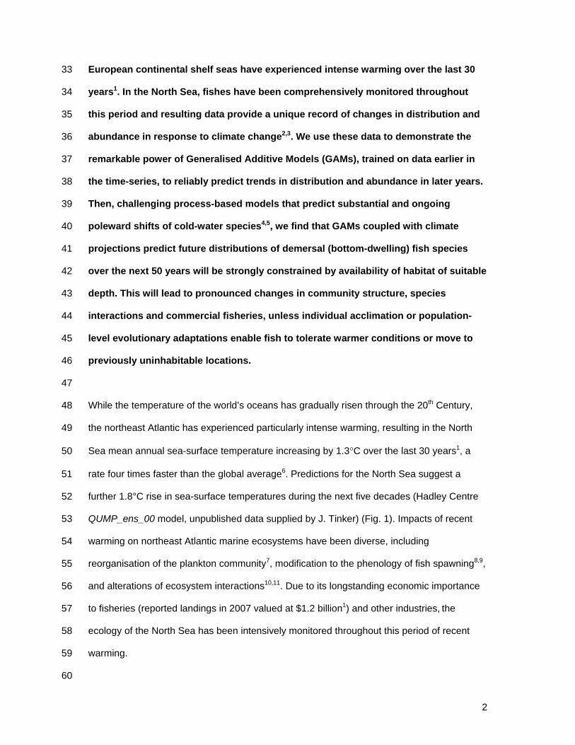
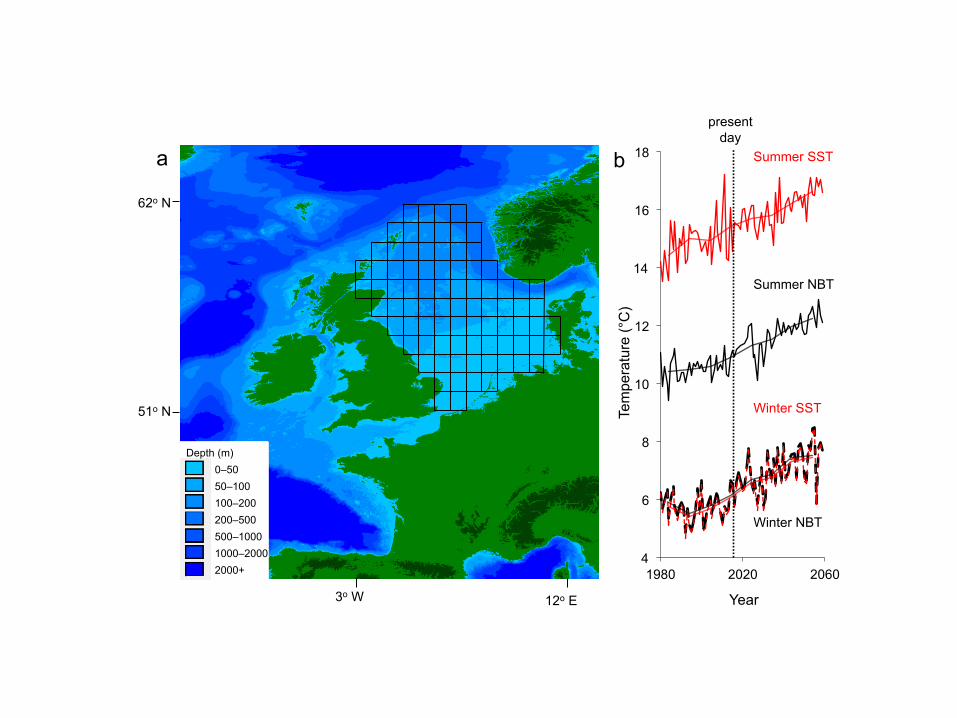
While the temperature of the world’s oceans has gradually risen through the 20th Century, 48

the northeast Atlantic has experienced particularly intense warming, resulting in the North 49

Sea mean annual sea-surface temperature increasing by 1.3°C over the last 30 years1, a 50

rate four times faster than the global average6. Predictions for the North Sea suggest a 51

further 1.8°C rise in sea-surface temperatures during the next five decades (Hadley Centre 52

QUMP_ens_00 model, unpublished data supplied by J. Tinker) (Fig. 1). Impacts of recent 53

warming on northeast Atlantic marine ecosystems have been diverse, including 54

reorganisation of the plankton community7, modification to the phenology of fish spawning8,9, 55

and alterations of ecosystem interactions10,11. Due to its longstanding economic importance 56

to fisheries (reported landings in 2007 valued at $1.2 billion1) and other industries, the 57

ecology of the North Sea has been intensively monitored throughout this period of recent 58

warming. 59

60

3

Analyses of North Sea fish surveys have revealed northerly range expansions of warmer-61

water species12, population redistributions to higher latitudes2 and deeper water13, and 62

widespread changes in local abundance associated with warming, with impacts on 63

community structure3. This substantial modification to fish community composition in the 64

region has had an observable economic impact on fisheries, with landings of cold-adapted 65

species halved but landings of warm-adapted species increasing 2.5 times since the 1980s3; 66

a pattern also identified in other marine ecosystems14. With a uniquely rich fish abundance 67

time-series from the period of warming, it is possible to split these data to assess how 68

predictions made using data from earlier years match observations from later years; a 69

validation approach which has been promoted for terrestrial systems15. Existing studies have 70

used survey data to describe past changes2,3,12,13, or adopted process-based climate 71

envelope models to predict future abundance without validation16. Thus there is a need to 72

compare the predictions of climate-envelope models with those from more structurally-73

complete data-driven models that have been developed and tested using spatially and 74

temporally explicit abundance data. 75

76

The GAM approach makes no a-priori assumptions about the nature of associations 77

between predictors and response variables17 and has been used to assess the importance 78

of different environmental drivers on patterns of distributions and relative abundance in 79

marine ecosystems18-20. Here we developed GAMs to predict changes in the distribution and 80

abundance of the 10 most abundant North Sea demersal (bottom-dwelling) fish species, 81

which accounted for 68% of commercial landings by the North Sea fishery between 1980 82

and 2010 (www.ices.dk/marine-data/dataset-collections/Pages/Fish-catch-and-stock-83

assessment.aspx). We used a two-step approach. First, predictive models with different sets 84

of variables were compared using data earlier in the time-series to train the models and 85

predict known distributions and abundances later in the time-series. Second, models were 86

used to predict changes in species distributions over the next 50 years. 87

88

4

Predictors of species’ abundance were identified from a wider array of potential variables 89

(annual sea-surface and near-bottom temperatures; seasonal sea-surface and near-bottom 90

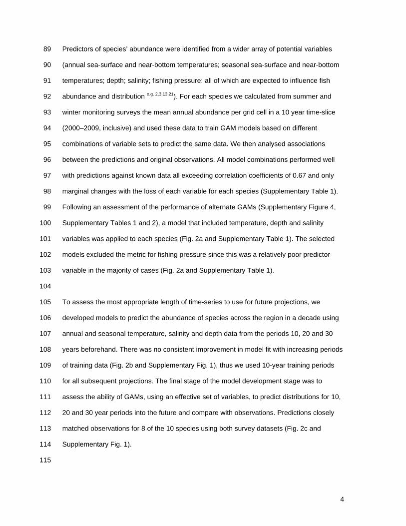
temperatures; depth; salinity; fishing pressure: all of which are expected to influence fish 91

abundance and distribution e.g. 2,3,13,21). For each species we calculated from summer and 92

winter monitoring surveys the mean annual abundance per grid cell in a 10 year time-slice 93

(2000–2009, inclusive) and used these data to train GAM models based on different 94

combinations of variable sets to predict the same data. We then analysed associations 95

between the predictions and original observations. All model combinations performed well 96

with predictions against known data all exceeding correlation coefficients of 0.67 and only 97

marginal changes with the loss of each variable for each species (Supplementary Table 1). 98

Following an assessment of the performance of alternate GAMs (Supplementary Figure 4, 99

Supplementary Tables 1 and 2), a model that included temperature, depth and salinity 100

variables was applied to each species (Fig. 2a and Supplementary Table 1). The selected 101

models excluded the metric for fishing pressure since this was a relatively poor predictor 102

variable in the majority of cases (Fig. 2a and Supplementary Table 1). 103

104

To assess the most appropriate length of time-series to use for future projections, we 105

developed models to predict the abundance of species across the region in a decade using 106

annual and seasonal temperature, salinity and depth data from the periods 10, 20 and 30 107

years beforehand. There was no consistent improvement in model fit with increasing periods 108

of training data (Fig. 2b and Supplementary Fig. 1), thus we used 10-year training periods 109

for all subsequent projections. The final stage of the model development stage was to 110

assess the ability of GAMs, using an effective set of variables, to predict distributions for 10, 111

20 and 30 year periods into the future and compare with observations. Predictions closely 112

matched observations for 8 of the 10 species using both survey datasets (Fig. 2c and 113

Supplementary Fig. 1). 114

115

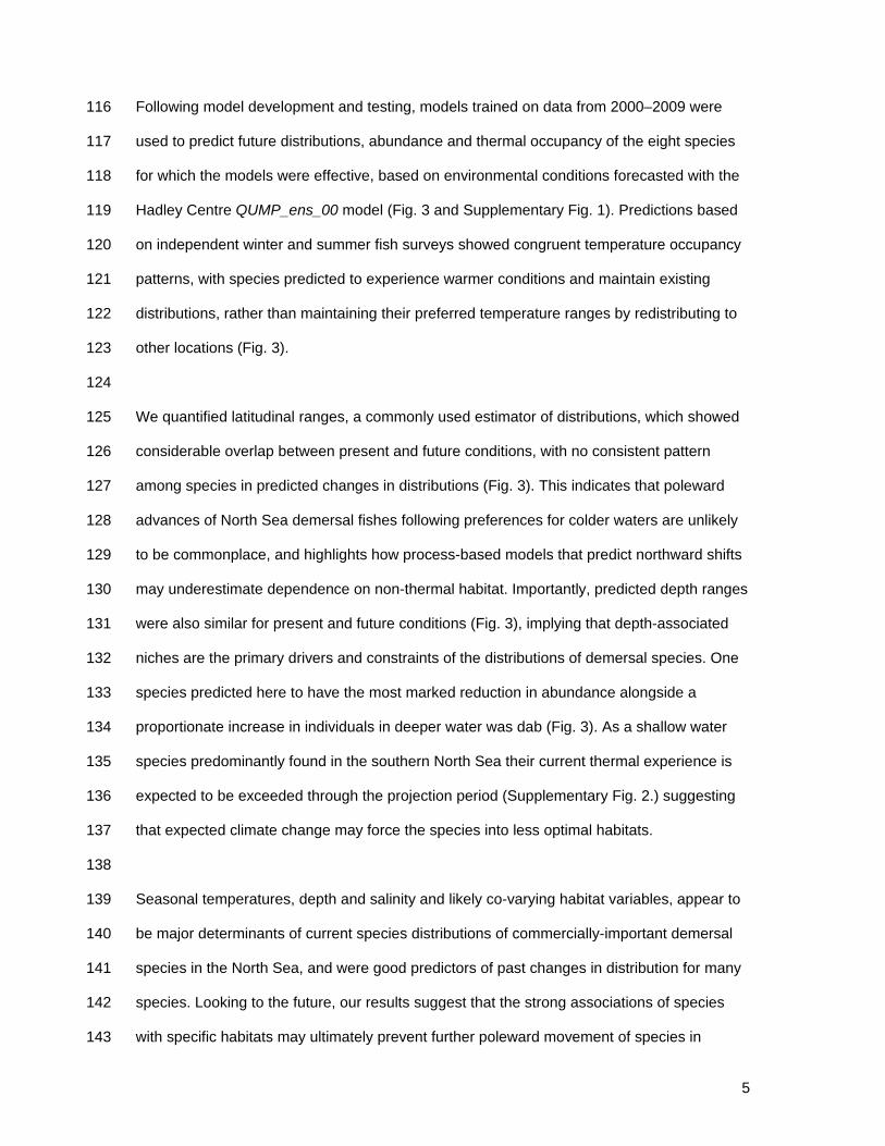
5

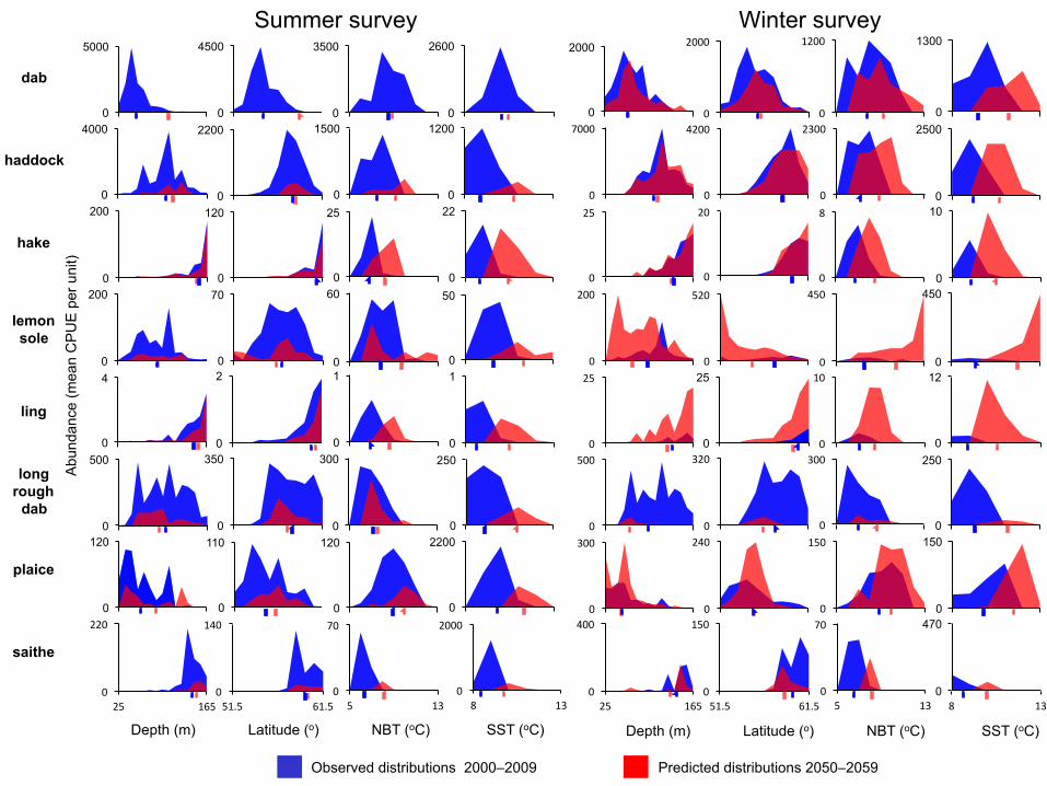
Following model development and testing, models trained on data from 2000–2009 were 116

used to predict future distributions, abundance and thermal occupancy of the eight species 117

for which the models were effective, based on environmental conditions forecasted with the 118

Hadley Centre QUMP_ens_00 model (Fig. 3 and Supplementary Fig. 1). Predictions based 119

on independent winter and summer fish surveys showed congruent temperature occupancy 120

patterns, with species predicted to experience warmer conditions and maintain existing 121

distributions, rather than maintaining their preferred temperature ranges by redistributing to 122

other locations (Fig. 3). 123

124

We quantified latitudinal ranges, a commonly used estimator of distributions, which showed 125

considerable overlap between present and future conditions, with no consistent pattern 126

among species in predicted changes in distributions (Fig. 3). This indicates that poleward 127

advances of North Sea demersal fishes following preferences for colder waters are unlikely 128

to be commonplace, and highlights how process-based models that predict northward shifts 129

may underestimate dependence on non-thermal habitat. Importantly, predicted depth ranges 130

were also similar for present and future conditions (Fig. 3), implying that depth-associated 131

niches are the primary drivers and constraints of the distributions of demersal species. One 132

species predicted here to have the most marked reduction in abundance alongside a 133

proportionate increase in individuals in deeper water was dab (Fig. 3). As a shallow water 134

species predominantly found in the southern North Sea their current thermal experience is 135

expected to be exceeded through the projection period (Supplementary Fig. 2.) suggesting 136

that expected climate change may force the species into less optimal habitats. 137

138

Seasonal temperatures, depth and salinity and likely co-varying habitat variables, appear to 139

be major determinants of current species distributions of commercially-important demersal 140

species in the North Sea, and were good predictors of past changes in distribution for many 141

species. Looking to the future, our results suggest that the strong associations of species 142

with specific habitats may ultimately prevent further poleward movement of species in 143

6

response to warming as previously predicted16. A recent study demonstrated that 1.6°C of 144

warming across the European continental shelf over the last 30 years locally favoured some 145

demersal species suited to warmer waters, but drove local declines in cold-adapted species, 146

despite long-term stability in spatial patterns of species presence-absence3. Dependence of 147

species on specific non-thermal habitat, together with spatially-contrasting local changes in 148

responses to warming3, may explain why mean latitudinal range shifts are only apparent in 149

some species2, and are not detected in others despite sharing similar temperature 150

preferences. Dependence on specific non-thermal habitat has been observed in tagged 151

Atlantic cod (Gadus morhua), where fish occupied suboptimal thermal habitat for extended 152

periods with likely costs to metabolism and somatic growth22. Indeed a dominant driver of 153

changes in the central distributions of cod in the North Sea appears to have been intense 154

fishing pressure over the last century rather than warming, which has depleted former 155

strongholds in the western North Sea, driving an eastward longitudinal shift in relative 156

population abundance but no apparent poleward shift21. These factors, together with 157

potential indirect effects of warming potentially not captured in our models, for example from 158

changes to prey abundance, may explain why models based on depth and temperature 159

were not effective for longer term projections for Atlantic cod and whiting (Merlangius 160

merlangus). It is necessary to evaluate the performance of alternate predictor variables for 161

data-driven models of these species. 162

163

Mean depth distributions of North Sea fishes that had preferences for cooler water increased 164

by approximately 5m during the warming of the 1980s but tended to slow or stabilise 165

thereafter13. Based on the GAM results we do not expect or predict substantial further 166

deepening for cooler water species because depth is such a strong predictor of distribution. 167

Collectively, the studies imply that capacity to remain in cooler water by changing their depth 168

distribution has been largely exhausted in the 1980s and that fish with preferences for cooler 169

water are being increasingly exposed to higher temperatures, with expected physiological, 170

life history and population consequences. 171

7

172

In the absence of substantial distributional shifts that would allow fish to occupy different 173

habitats and depths, North Sea populations are likely to experience 3.2°C of warming over 174

the coming century (J. Tinker, Hadley Centre). Although such temperature increases are 175

within observed thermal limits for these species the ecological consequences are unknown, 176

especially when warmer conditions are closer to thermal preferences of other species using 177

the same habitats. Furthermore, physiological theory suggests that responses of species to 178

projected warming will eventually reach thermal thresholds. As species’ Pejus temperatures 179

are reached, increased metabolic costs will compromise growth with associated declines in 180

population productivity23. Capacity to tolerate warming will thus depend on scope for thermal 181

acclimation24 and adaptation25, with the degree of connectivity between thermally-adapted 182

sub-populations across the geographic range of species influencing the rate of adaptation to 183

future warming. Unless adaptation or acclimation can track the rate of warming, it is likely 184

that stocks will be affected, both directly through individual physiological tolerances, and 185

indirectly through climate-related changes to the abundance of prey, predators, competitors 186

and pathogens. 187

188

Our study demonstrates the power of data-driven GAM models for predicting future fish 189

distributions. In contrast to process-based models that attempt to integrate discrete 190

ecological mechanisms such as dispersal and density dependence, GAMs are grounded by 191

past net responses of populations to all these processes, in addition to interspecific 192

interactions and habitat associations that are not typically considered in process-based 193

modelling, perhaps explaining the strong predictive power of our GAM approach for 194

predicting known future conditions. The results of this study suggest that we should be 195

cautious when interpreting process-based model projections of distributional shifts, and that 196

interpretations should be informed by data-driven modelling approaches, especially when 197

using predictions for policy and management planning. Our projections suggest that if 198

populations fail to adapt or acclimatise to a warmer environment, warming will change 199

8

fishing opportunities for currently-targeted species in the North Sea over the next century. 200

Historically, fishing pressure has substantially modified the North Sea26 and ongoing 201

changes in management will play an important role in shaping future fisheries resources. 202

Species responses to temperature should be considered when planning future fisheries 203

management strategies to ensure that anticipated long-term benefits of management are 204

ecologically feasible in this period of intense warming. 205

206

METHODS 207

Fish surveys. We used two long-term monitoring surveys that give detailed descriptions of 208

the distribution and abundance of demersal (bottom-dwelling) fishes in the North Sea. The 209

Centre for Environment, Fisheries and Aquaculture Science UK (Cefas) time-series is a 210

summer survey (August–September) conducted since 1980. The survey encompasses 69 211

1x1° latitude-longitude cells with at least three hauls conducted in each decade. The 212

International Council for the Exploration of the Sea (ICES) International Bottom Trawl Survey 213

(IBTS) time-series is a winter survey (January–March) conducted since 1980. The survey 214

encompasses 84 1x1° cells with at least three hauls conducted in each decade. Both 215

surveys are conducted using otter trawling gear (Granton trawl for pre-1992 Cefas surveys, 216

otherwise Grande Ouverture Verticale (GOV) trawls). Raw catch data were 4th-root 217

transformed to reduce skewness that is inherent in ecological abundance data. 218

219

Our study focused on the 10 most abundant demersal species targeted by commercial 220

fisheries or taken as bycatch (Fig. 2c), which together accounted for 68% of commercial 221

landings (by weight) in the North Sea fishery from 1980–2010 (www.ices.dk/marine-222

data/dataset-collections/Pages/Fish-catch-and-stock-assessment.aspx). For both surveys, 223

we grouped data into three 10-year time slices and one three-year time slice for the 224

analyses: 1980–1989, 1990–1999, 2000–2009 and 2010–2012. The limited 2010–2012 time 225

slice was only used for testing predictions from the GAMs. To ensure a balanced design, 226

9

mean values for each for each decadal time period were used. This method controls for the 227

variable numbers of survey hauls taken in each cell and ensures that longer-term responses 228

to climate change are identified rather than year on year variability. All data were 4th root 229

transformed before being subject to GAM modelling, and individual cell predictions were 230

back transformed before calculation of correlation coefficients. 231

232

Depth. We used mean 1x1° cell in situ measures of depth taken during the hauls for each 233

survey (Supplementary Fig. 3), which closely matched data from the 1x1o resolution GEBCO 234

Digital Atlas (summer survey, r = 0.91; winter survey, r = 0.90; 235

www.gebco.net/data_and_products/gebco_digital_atlas/)3. 236

237

Temperature and salinity. We calculated Sea-Surface Temperature (SST), Near-Bottom 238

Temperature (NBT) and salinity (Supplementary Fig. 3) for the period 1980–2012 using the 239

UK Meteorological Office Hadley Centre QUMP_ens_00 standard model for the northwest 240

European shelf seas. Modelled temperatures closely matched data from the Hadley Centre 241

global ocean surface temperature database (HadISST1.1; 92 cells, Pearson’s r = 0.84; 242

www.metoffice.gov.uk/hadobs/hadisst/). Data from the QUMP_ens_00 model were provided 243

as monthly means for 1x1° cells, enabling mean winter (January–March), summer (July–244

September) and mean annual values to be calculated (Fig. 1). 245

246

Fishing pressure. We calculated a spatially-explicit metric of fishing pressure for each 10-247

year time-slice by combining annual multispecies fishing mortality (F) estimates for North 248

Sea demersal species (mean estimates of regional F for cod, dab, haddock, hake, lemon 249

sole, ling, long rough dab, plaice, saithe and whiting, weighted by spawning-stock biomass, 250

from ICES stock assessments; www.ices.dk/datacentre/StdGraphDB.asp)3 with mean otter 251

and beam trawling effort for each 1x1° cell based on hours of fishing27 (Supplementary Fig. 252

3). This integrated metric combining temporal trends in fishing mortality and spatial 253

10

distribution of fishing effort enabled us to test the importance of fishing pressure as a 254

predictor of abundance. 255

256

Identifying key predictors. We used GAM models, coded using the mgcv package in R 257

(www.r-project.org), to test the performance of GAMs for predicting changes in fish species’ 258

distribution and identify the importance of different variables to these predictions. The s 259

smooth was used with k = 7 for all variables to limit the degrees freedom in-line with the 260

number of data points. The Gaussian model was used. Assessment of the plots for each 261

variable using the gam.plot function showed that increasing the k value did not improve 262

model fit to each variable. The gam.check function was used to check the k index was above 263

or close to 1 with non-significant p values. Analysis of the residuals showed no obvious 264

deviations from normal distributions, while the response to fitted values relationship was 265

close to linear. 266

267

Data from 2000–2009 were used to test sets of variables as this period had the greatest 268

survey intensity. To identify variables that most strongly influenced prediction we first 269

developed a model with all variables (annual temperatures, seasonal temperatures, depth, 270

salinity and fishing), and a subsequent five models each excluding one set of variables 271

(Supplementary Table 1). Sea surface and near bottom temperatures from both the summer 272

and winter were grouped together to characterise seasonal fluctuations. This suite of 273

potentially correlated variables captured the extremes of temperatures that all species may 274

experience at different life stages, and ensured that thermal conditions with and without the 275

seasonal thermocline, annually varying ocean currents and land mass effects are all 276

included. We compared the performance of models based on i) the strength of correlation r 277

between observed and predicted data, ii) weighted AIC 28 using data from the AIC function in 278

R, and iii) using generalised cross validation (GCV, through summary.gam in R). Inclusion of 279

interaction terms between depth and seasonal temperature extremes either reduced or had 280

little influence on model performance (Supplementary Table 2 and summaries based on 281

11

Akaike weights in Supplementary Fig. 4). 282

283

Model development 284

We developed predictive GAMs with a set of variables that were effective across all species. 285

The correlation coefficient r, AIC values and GCV values of modelled and observed data 286

were compared. Across-species inclusion of depth, seasonal temperature, annual 287

temperature, salinity and fishing effort all improved the predictions (Fig. 2a). A key finding 288

from this model development stage is that variables that are readily measured and projected 289

in climate models effectively predict species distributions. On average models that excluded 290

fishing effort were most similar to the all-variable models (Supplementary Table. 1, Fig. 2a). 291

Since this metric had little predictive value, and we have no robust models of future fishing 292

effort, we excluded it when making future predictions. 293

294

Training period and predictive performance. To assess the influence of the duration of 295

training data on predictive power, GAMs trained on sets of one, two and three decades of 296

data for each species were used to predict 10 years into the future (Supplementary Fig. 1), 297

and the associations between predicted and known data compared. We also assessed the 298

performance of the model to predict further into the future within the historic records 299

available (Supplementary Fig. 1). We compared predicted with known abundance data for 300

each species for each forecasting period (0 to 30 years). 301

302

Forecasting future distributions. We used surface and near bottom annual and seasonal 303

temperature projections from the QUMP_ens_00 model, surface and near bottom salinity, 304

and average depths from surveys between 1980–2012 as the environmental variables for 305

our predictions. We predicted fish abundances for sequential decades from 2000–2009 to 306

2050–2059 (Supplementary Figs. 5 & 6) using environmental variables (Supplementary 307

Figs. 3 & 7), and observed fish abundances from 2000–2009. Throughout the projection 308

period many cells do not experience temperatures outside of the range used to train the 309

12

model (Supplementary Fig. 2). For the widespread species in this study it is therefore likely 310

that at least parts of the population have experienced future conditions. However we 311

recognise that in future projected conditions the climate in some areas of the North Sea will 312

depart from existing variability in the model training period. Since it is not possible to test the 313

model beyond current thermal conditions using know data, some caution should be taken 314

interpreting projections for cells as they begin to experience temperatures beyond those 315

currently in the region (Supplementary Fig. 2). 316

317

REFERENCES 318

1 Sherman, K. and Hempel, G. (Editors). The UNEP Large Marine Ecosystem Report: 319

A perspective on changing conditions in LMEs of the world’s Regional Seas. UNEP 320

Regional Seas Report and Studies No. 182. United Nations Environment 321

Programme. Nairobi, Kenya (2009). 322

2 Perry, A. L., Low, P. J., Ellis, J. R. & Reynolds, J. D. Climate change and distribution 323

shifts in marine fishes. Science 308, 1912–1915 (2005). 324

3 Simpson, S. D. et al. Continental shelf-wide response of a fish assemblage to rapid 325

warming of the sea. Curr. Biol. 21, 1565–1570 (2011). 326

4 Cheung, W. W., Lam, V. W., Sarmiento, J. L., Kearney, K., Watson, R. & Pauly, D. 327

Projecting global marine biodiversity impacts under climate change scenarios. Fish 328

Fish. 10, 235–251 (2009). 329

5 Jones, M. C. et al. Predicting the impact of climate change on threatened species in 330

UK waters. PLoS ONE 8, e54216 (2013). 331

6 Smith, T. M., Reynolds, R. W., Peterson, T. C. & Lawrimore, J. Improvements to 332

NOAA's historical merged land-ocean surface temperature analysis (1880–2006). J. 333

Climate 21, 2283–2296 (2008). 334

13

7 Beaugrand, G., Reid, P. C., Ibanez, F., Lindley, J. A. & Edwards, M. Reorganization 335

of North Atlantic marine copepod biodiversity and climate. Science 296, 1692–1694 336

(2002). 337

8 Edwards, M. & Richardson, A. J. Impact of climate change on marine pelagic 338

phenology and trophic mismatch. Nature 430, 881–884 (2004). 339

9 Genner, M. J. et al. Temperature-driven phenological changes within a marine larval 340

fish assemblage. J. Plankton Res. 32, 699–708 (2010). 341

10 Beaugrand, G., Brander, K. M., Lindley, J. A., Souissi, S. & Reid, P. C. Plankton 342

effect on cod recruitment in the North Sea. Nature 426, 661–664 (2003). 343

11 Durant, J. M., Hjermann, D. O., Ottersen, G. & Stenseth, N. C. Climate and the 344

match or mismatch between predator requirements and resource availability. Climate 345

Res. 33, 271–283 (2007). 346

12 Beare, D. J. et al. Long-term increases in prevalence of North Sea fishes having 347

southern biogeographic affinities. Mar. Ecol. Prog. Ser. 284, 269–278 (2004). 348

13 Dulvy, N. K. et al. Climate change and deepening of the North Sea fish assemblage: 349

a biotic indicator of warming seas. J. Appl. Ecol. 45, 1029–1039 (2008). 350

14 Cheung, W. W. L., Watson, R. & Pauly, D. Signature of ocean warming in global 351

fisheries catch. Nature 497, 365–369 (2013). 352

15 Araujo, M. B., Pearson, R. G., Thuiller, W. & Erhard, M. Validation of species-climate 353

impact models under climate change. Glob. Change Biol. 11, 1504–1513 (2005). 354

16 Cheung, W. W. L. et al. Large-scale redistribution of maximum fisheries catch 355

potential in the global ocean under climate change. Glob. Change Biol. 16, 24–35 356

(2010). 357

17 de Madron, X. D. et al. Marine ecosystems' responses to climatic and anthropogenic 358

forcings in the Mediterranean. Prog. Oceanogr. 91, 97–166 (2011). 359

18 Dingsor, G. E., Ciannelli, L., Chan, K.-S., Ottersen, G. & Stenseth, N. C. Density 360

dependence and density independence during the early life stages of four marine fish 361

stocks. Ecology 88, 625–634 (2007). 362

14

19 Hedger, R. et al. Analysis of the spatial distributions of mature cod (Gadus morhua) 363

and haddock (Melanogrammus aeglefinus) abundance in the North Sea (1980–1999) 364

using generalised additive models. Fish. Res. 70, 17–25 (2004). 365

20 Belanger, C. L. et al. Global environmental predictors of benthic marine 366

biogeographic structure. P. Natl. Acad. Sci. USA 109, 14046–14051 (2012). 367

21 Engelhard, G. H., Righton, D. A. and Pinnegar, J. K. Climate change and fishing: a 368

century of shifting distribution in North Sea cod. Glob. Change Biol. 20, 2473–2483 369

(2014). 370

22 Neat, F. C. & Righton, D. Warm water occupancy by North Sea cod. P. Roy. Soc. 371

Lond. B Bio. 274, 789–798 (2007). 372

23 Neuheimer, A. B., Thresher, R. E., Lyle, J. M. & Semmens, J. M. Tolerance limit for 373

fish growth exceeded by warming waters. Nature Clim. Change 1, 110–113 (2011). 374

24 Donelson, J. M., Munday, P. L., McCormick, M. I. & Pitcher, C. R. Rapid 375

transgenerational acclimation of a tropical reef fish to climate change. Nature Clim. 376

Change 2, 30–32, (2012). 377

25 Crozier, L. G. & Hutchings, J. A. Plastic and evolutionary responses to climate 378

change in fish. Evol. Apps. 7, 68–87 (2014). 379

26 Jennings, S. & Blanchard, J. L. Fish abundance with no fishing: predictions based on 380

macroecological theory. J. Anim. Ecol. 73, 632–642 (2004). 381

27 Jennings, S. et al. Fishing effects in northeast Atlantic shelf seas: patterns in fishing 382

effort, diversity and community structure. III. International trawling effort in the North 383

Sea: an analysis of spatial and temporal trends. Fish. Res. 40, 125–134 (1999). 384

28 Burnham, K. P. and D. R. Anderson. Model Selection and Multimodel Inference. 385

(Springer-Verlag, New York, 2002). 386

387

AUTHOR INFORMATION 388

Correspondence and requests for materials should be addressed to S.D.S. 389

(S.Simpson@exeter.ac.uk). 390

15

391

ACKNOWLEDGEMENTS 392

We thank staff of the Centre for Environment, Fisheries and Aquaculture Science UK 393

(Cefas) and all contributors to the International Council for the Exploration of the Sea (ICES) 394

International Bottom Trawl Survey (IBTS) for collecting and providing survey data. We thank 395

Sandrine Vaz for training in GAM modeling in R and David Maxwell for statistical guidance. 396

This work was supported by a Natural Environment Research Council (NERC) / Department 397

for Environment Food and Rural Affairs (Defra) Sustainable Marine Bioresources award 398

(NE/F001878/1), with additional support from a NERC KE Fellowship (S.D.S; 399

NE/J500616/2), NERC-Cefas CASE PhD Studentship (L.A.R; NE/L501669/1), Great 400

Western Research (M.J.G.), Defra (S.J. and J.L.B.), NERC Oceans 2025 (M.J.G. and 401

D.W.S), The Worshipful Company of Fishmongers (D.W.S.), and a Marine Biological 402

Association Senior Research Fellowship (D.W.S.). 403

404

AUTHOR CONTRIBUTIONS 405

M.J.G. and M.P.J. conceived the research; S.J., J.L.B. and D.W.S. contributed to project 406

development; S.D.S. and S.J. pre-processed fisheries agency data; L.A.R. and J.T. pre-407

processed climate data; S.D.S., M.J.G., L.A.R., M.P.J. and S.J. designed the analysis; L.A.R 408

and S.D.S. conducted the analysis; S.D.S., L.A.R and M.J.G. prepared the initial manuscript 409

and all authors contributed to revisions. 410

411

COMPETING FINANCIAL INTERESTS STATEMENT 412

The authors declare no competing financial interests. 413

414

415

FIGURE LEGENDS 416

417

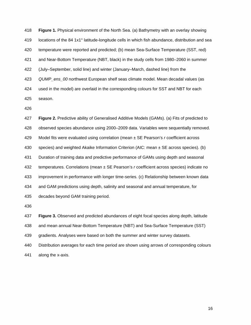
16

Figure 1. Physical environment of the North Sea. (a) Bathymetry with an overlay showing 418

locations of the 84 1x1° latitude-longitude cells in which fish abundance, distribution and sea 419

temperature were reported and predicted; (b) mean Sea-Surface Temperature (SST, red) 420

and Near-Bottom Temperature (NBT, black) in the study cells from 1980–2060 in summer 421

(July–September, solid line) and winter (January–March, dashed line) from the 422

QUMP_ens_00 northwest European shelf seas climate model. Mean decadal values (as 423

used in the model) are overlaid in the corresponding colours for SST and NBT for each 424

season. 425

426

Figure 2. Predictive ability of Generalised Additive Models (GAMs). (a) Fits of predicted to 427

observed species abundance using 2000–2009 data. Variables were sequentially removed. 428

Model fits were evaluated using correlation (mean ± SE Pearson’s r coefficient across 429

species) and weighted Akaike Information Criterion (AIC: mean ± SE across species). (b) 430

Duration of training data and predictive performance of GAMs using depth and seasonal 431

temperatures. Correlations (mean ± SE Pearson’s r coefficient across species) indicate no 432

improvement in performance with longer time-series. (c) Relationship between known data 433

and GAM predictions using depth, salinity and seasonal and annual temperature, for 434

decades beyond GAM training period. 435

436

Figure 3. Observed and predicted abundances of eight focal species along depth, latitude 437

and mean annual Near-Bottom Temperature (NBT) and Sea-Surface Temperature (SST) 438

gradients. Analyses were based on both the summer and winter survey datasets. 439

Distribution averages for each time period are shown using arrows of corresponding colours 440

along the x-axis. 441

4

6

8

10

12

14

16

18

1980 2020 2060

b a

Depth (m) 0 1000 2000 3000 4000 5000 6000 7000

Tem

pera

ture

(°C

)

1000–2000

0–50

100–200

500–1000

200–500

50–100

2000+

Depth (m)

62o N

51o N

3o W 12o E Year

Summer SST Summer NBT

Winter SST

Winter NBT

present day

-0.5

0

0.5

1

0 10 20 30 -0.5

0

0.5

1

0 10 20 30

cod dab haddock hake lemon sole ling long rough dab plaice saithe whiting

Prediction into future (years)

Cor

rela

tion

(r) o

f obs

erve

d an

d m

odel

led

abun

danc

e

GAM training period (years)

Blue (bottom axis): Correlation (r) of observed and modelled abundance. Red (top axis): Weighted AIC values of models

a

b

c

Winter survey Summer survey

0.4

0.5

0.6

0.7

0.8

0.9

10 20 30 0.4

0.5

0.6

0.7

0.8

0.9

10 20 30

Cor

rela

tion

(r) o

f obs

erve

d an

d m

odel

led

abun

danc

e

0.8 1

Excluding fishing

Excluding salinity

Excluding depth

Excluding seasonal temperature

Excluding annual temperature

All variables

0 0.5

All variables

Excluding annual temperature

Excluding seasonal temperature

Excluding depth Excluding salinity Excluding fishing !

0.8 1

0 0.5

0"

140"

51.5" 61.5"

0

120

0

2200

0

120

0

70

0

2

0

350

0

4500

0

22

0

50

0

1

0

250

0

2200

0

2600

0

120

0"

220"

25" 165"

0

4000

0

200

0

4

0

5000

0

1300

0

25

0

12

0"

400"

25" 165"0

470

8" 13"0"

70"

5" 13"0"

2000"

8" 13"

0"

200"

0

110

0

1500

0

25

0

60

0

1

0

300

0

3500

0

1200 0

2000

0"

7000"

0"

25"

0"

25"

0"

500"

0"

300"

0"

4200"

0"

20"

0"

520"

0"

320"

0"

240"

0"

2000"

0"

2300"

0"

8"

0"

450"

0"

10"

0"

300"

0"

150"

0"

1200"

0

2500

0

10

0

450

0

250

0

150

0"

150"

51.5" 61.5"0"

70"

5" 13"

Depth (m) Latitude (o) NBT (oC) SST (oC)

0

200

0

500

Depth (m) Latitude (o) NBT (oC) SST (oC)

Summer survey Winter survey

dab

haddock

hake

lemon sole

ling

long rough

dab

plaice

saithe

Abu

ndan

ce (m

ean

CP

UE

per

uni

t)

Observed distributions 2000–2009 Predicted distributions 2050–2059