INSTITUTE OF PHYSICS PUBLISHING COMBUSTION THEORY AND MODELLING

Combust. Theory Modelling 8 (2004) 1–22 PII: S1364-7830(04)61306-4

PDF calculations of turbulent lifted flames of H2/N2fuel issuing into a vitiated co-flow

A R Masri1,4, R Cao2, S B Pope2 and G M Goldin3

1 School of Aerospace, Mechanical and Mechatronic Engineering, The University of Sydney,NSW 2006, Australia2 Mechanical and Aerospace Engineering, Cornell University, Ithaca, NY 14850, USA3 Fluent Inc, Lebanon, New Hampshire, USA

Received 25 March 2003, in final form 10 October 2003Published 13 November 2003Online at stacks.iop.org/CTM/8/1 (DOI: 10.1088/1364-7830/8/1/001)

AbstractThis paper presents detailed calculations of the flow, mixing and compositionfields of a simple jet of hydrogen–nitrogen mixture issuing into a vitiatedco-flowing stream. The co-flow contains oxygen as well as combustion productsand is sufficiently hot to provide an ignition source for a flame that stabilizesat some ten diameters downstream of the jet exit plane. This configurationforms a good model problem for studying lifted flames as well as issues ofauto-ignition.

The calculations employ a composition probability density function (PDF)approach coupled to the commercial CFD package FLUENT. The in situadaptive tabulation method is adopted to account for detailed chemical kinetics.A simple k–ε model is used for turbulence along with a low Reynolds numbermodel for the walls. Calculations are optimized to obtain a numerically accuratesolution and are repeated for two different H2 mechanisms, each consisting often species. The flame is found to be largely controlled by chemical rather thanmixing processes. The mechanisms used yield different lift-off heights andcompositions that straddle the data. Ignition delays are found to be extremelysensitive to the chemical kinetic rates of some reactions in the mechanisms.

(Some figures in this article are in colour only in the electronic version)

1. Introduction

Despite the apparent simplicity of the flow, lifted flames continue to pose a challenge tomodellers due to the outstanding difficulty in understanding the stabilization processes. Thereare many theories and hypotheses proposed for lifted flame stabilization [1, 2], all of whichremain unproven due to the lack of reliable data. A comprehensive review of flame stabilizationtheories may be found in Pitts [3]. Until recently, only global measurements of lift-off heightswere available and these were used to generate empirical correlations for lifted flames [4–9].

4 Author to whom any correspondence should be addressed.

1364-7830/04/010001+22$30.00 © 2004 IOP Publishing Ltd Printed in the UK 1

2 A R Masri et al

However, this scenario is gradually changing and detailed single point data as well as planarimages of a range of scalars taken at the base of lifted flames have recently appeared in[10–13]. The difficulty, both experimentally and numerically, lies in the fact that the flameat the stabilization base is unstable and involves a significant degree of interaction betweenchemical and flow timescales. Spontaneously, the flame zone appears to reside where a balancebetween these interacting processes is reached [11]. Accounting for such interactions requiresthe use of detailed chemical kinetics as well as correct representation of the flow-field.

In a recent breakthrough in the computation of turbulent non-premixed combustion,Tang et al [14] and Lindstedt et al [15] have used the probability density function (PDF)approach with detailed chemical kinetics to compute extinction and re-ignition processes inpilot-stabilized diffusion flames. Although the approaches of the two groups differ in the useof mixing models, chemical kinetics and its implementation, they constitute the first directand detailed computations of finite-rate chemistry effects in diffusion flames. Lindstedt andLouloudi [16] have recently extended the approach to piloted flames of methanol fuel while Liuet al [17] have performed successful computations of finite-rate chemistry effects in the morecomplex bluff-body stabilized flames of methane–hydrogen fuels. Conditional moment closureapproaches [18–20] are gradually developing capabilities for computing finite-rate chemistryeffects with the introduction of second order methods or second level of conditioning. However,large eddy simulations [21] remain largely constrained by huge computational requirements.

Another issue that is relevant to lifted flames as well as to engine combustion in general isthe auto-ignition that occurs when reactive mixtures encounter hot pockets of air or combustionproducts. The chemical reactions that control auto-ignition may not necessarily be the sameas those controlling steady combustion. In the flames considered here, the flames are largelycontrolled by chemical kinetics and hence the correct representation of the chemistry is critical.Numerical and theoretical studies of auto-ignition [22–28] have shown that mixtures do notnecessarily ignite at stoichiometric mixture fraction but rather at mixture fractions wherethe fluid is most reactive yet the scalar dissipation rate is relatively low. Direct numericalsimulations are proving to be an extremely useful tool in furthering current understanding ofauto-ignition [24–28]. However, laboratory experiments investigating this phenomenon arerather scarce. Dally et al [29] have presented a detailed experimental study of a turbulent jetof H2/CH4 issuing into a stream of hot combustion products where the oxygen level is varied.Although this flow configuration is referred to as flameless or moderate and intense low oxygendilution (MILD) combustion, it is closely related to auto-ignition.

This paper addresses both issues of auto-ignition and lifted flame stabilization. It presentscalculations for turbulent jets of H2/N2 issuing in a wide co-flow of hot gas mixtures. The jetfluid mixes with co-flowing combustion products and heated air and subsequently auto-ignites,forming a lifted flame stabilized at about ten jet diameters downstream of the exit plane. Thisburner, developed by Cabra et al [30], has the advantage of representing both lift-off andauto-ignition in a rather simple and well-defined flow configuration. However, it should benoted that lifted flames issuing in vitiated co-flow are different from those stabilized in stillair. The temperature and composition of the co-flow impose different conditions such that thecontrolling processes and the dynamics of flame stabilization are different from a regular liftedflame. Extensive composition data have been provided by Cabra [31] and these are used herefor comparisons with the calculations.

2. The burner

Figure 1 shows a schematic of the burner and the computational domain used in the currentcalculations. The fuel jet, which has an inner diameter D = 4.57 mm and a wall thickness of

PDF calculations of turbulent lifted flames of H2/N2 fuel 3

(a) (b)

Figure 1. Schematic of (a) the burner and (b) the computational domain.

Table 1. Experimental conditions for the reacting and non-reacting jets.

Non-reacting case Reacting case

Jet Pilot Jet Pilot

Velocity (m s−1) 170 4.4 107 3.5ξs — — 0.47 —� — 0.31 — 0.25T (K) 310 1190 305 1045X(O2) 0.21 0.135 0 0.1474X(N2) 0.79 0.741 0.75 0.7532X(H2O) 0 0.124 0 0.0989X(H2) 0 0 0.25 0X(OH) 0 0 0 0.0005

0.89 mm, is located at the centre of a perforated disc that has a diameter of 210 mm. The dischas 2200 × 1.58 mm diameter holes that stabilize as many premixed flames, providing a hotco-flowing stream with a temperature and composition that are outlined in table 1. The overallblockage of the perforated plate is 87%. The central fuel jet extends by 70 mm downstreamof the surface of the perforated plate so that the fuel mixture exits in a uniform compositionfor the co-flow. The entire burner assembly is shrouded with a water jacket for cooling andsits in stagnant air. The surrounding air does not affect the central jet for the axial locationsdiscussed in this paper (which extend to about x/D = 26).

Two sets of measurements are available for this flow configuration, one for a non-reactingjet of air and the other for a lifted flame, both issuing in a vitiated co-flow. The burner waslocated in the wind tunnel at the Combustion Research Facility, Sandia National Laboratories,where detailed single point measurements of temperature and composition were made usingthe Raman–Rayleigh–LIF technique. The mass fractions of N2, O2, H2O, OH and NO weremeasured and the data have been made available by Sreedhara and Lakshmisha [24]. Furtherdetails of the measurement technique, calibration and accuracy of the data may be foundelsewhere [30]. Measurements of the flow-field are not yet available. Details of the conditionsand characteristics of both cases are shown in table 1.

3. PDF computations

All computations presented here use the FLUENT package, which solves Reynolds averagedNavier–Stokes (RANS) equations for the mean conservation of mass, momentum and energy,

4 A R Masri et al

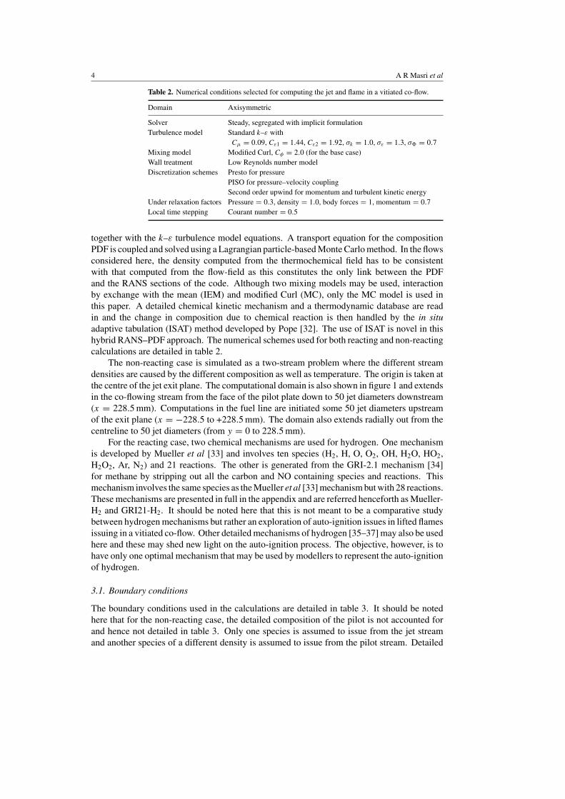
Table 2. Numerical conditions selected for computing the jet and flame in a vitiated co-flow.

Domain Axisymmetric

Solver Steady, segregated with implicit formulationTurbulence model Standard k–ε with

Cµ = 0.09, Cε1 = 1.44, Cε2 = 1.92, σk = 1.0, σε = 1.3, σ� = 0.7Mixing model Modified Curl, Cφ = 2.0 (for the base case)Wall treatment Low Reynolds number modelDiscretization schemes Presto for pressure

PISO for pressure–velocity couplingSecond order upwind for momentum and turbulent kinetic energy

Under relaxation factors Pressure = 0.3, density = 1.0, body forces = 1, momentum = 0.7Local time stepping Courant number = 0.5

together with the k–ε turbulence model equations. A transport equation for the compositionPDF is coupled and solved using a Lagrangian particle-based Monte Carlo method. In the flowsconsidered here, the density computed from the thermochemical field has to be consistentwith that computed from the flow-field as this constitutes the only link between the PDFand the RANS sections of the code. Although two mixing models may be used, interactionby exchange with the mean (IEM) and modified Curl (MC), only the MC model is used inthis paper. A detailed chemical kinetic mechanism and a thermodynamic database are readin and the change in composition due to chemical reaction is then handled by the in situadaptive tabulation (ISAT) method developed by Pope [32]. The use of ISAT is novel in thishybrid RANS–PDF approach. The numerical schemes used for both reacting and non-reactingcalculations are detailed in table 2.

The non-reacting case is simulated as a two-stream problem where the different streamdensities are caused by the different composition as well as temperature. The origin is taken atthe centre of the jet exit plane. The computational domain is also shown in figure 1 and extendsin the co-flowing stream from the face of the pilot plate down to 50 jet diameters downstream(x = 228.5 mm). Computations in the fuel line are initiated some 50 jet diameters upstreamof the exit plane (x = −228.5 to +228.5 mm). The domain also extends radially out from thecentreline to 50 jet diameters (from y = 0 to 228.5 mm).

For the reacting case, two chemical mechanisms are used for hydrogen. One mechanismis developed by Mueller et al [33] and involves ten species (H2, H, O, O2, OH, H2O, HO2,H2O2, Ar, N2) and 21 reactions. The other is generated from the GRI-2.1 mechanism [34]for methane by stripping out all the carbon and NO containing species and reactions. Thismechanism involves the same species as the Mueller et al [33] mechanism but with 28 reactions.These mechanisms are presented in full in the appendix and are referred henceforth as Mueller-H2 and GRI21-H2. It should be noted here that this is not meant to be a comparative studybetween hydrogen mechanisms but rather an exploration of auto-ignition issues in lifted flamesissuing in a vitiated co-flow. Other detailed mechanisms of hydrogen [35–37] may also be usedhere and these may shed new light on the auto-ignition process. The objective, however, is tohave only one optimal mechanism that may be used by modellers to represent the auto-ignitionof hydrogen.

3.1. Boundary conditions

The boundary conditions used in the calculations are detailed in table 3. It should be notedhere that for the non-reacting case, the detailed composition of the pilot is not accounted forand hence not detailed in table 3. Only one species is assumed to issue from the jet streamand another species of a different density is assumed to issue from the pilot stream. Detailed

PDF calculations of turbulent lifted flames of H2/N2 fuel 5

Table 3. Boundary conditions for the non-reacting and reacting jets.

Stream Condition Non-reacting jet Lifted flame

Fuel jet Velocity (m s−1) 170 107Turbulent kinetic energy (m2 s−2) 1.0 1.0Turbulence dissipation rate (m2 s−3) 1.0 1.0Temperature (K) 310 305Y(H2) — 0.023 44Y(Ar) — 0.01Density, ρ (kg m−3) 0.854 0.859

Pilot co-flow Velocity (m s−1) 4.4 3.5Turbulent intensity (%) 5.0 5.0Turbulence length scale (mm) 1.0 1.0Temperature (K) 1190 1045Y(O2) — 0.170 92Y(OH) — 0.000 31Y(H2O) — 0.064 56Density, ρ (kg m−3) 0.322 0.322

Jet wall Wall with zero heat flux (adiabatic)Outer wall SymmetryOutflow Pressure outlet

Table 4. Relevant information about the various meshes used in the calculations.

X Y Mesh 1 Mesh 2 Mesh 3

From To From To Cells Cells Cells Cells Cells Cells(mm) (mm) (mm) (mm) X Y X Y X Y

Fuel jet −228.5 0 0 2.285 27 5 54 10 108 20Pilot stream A −70 0 2.285 60 11 31 22 62 44 124Pilot stream B −70 0 60 228.5 11 14 22 28 44 28Main domain A 0 228.5 0 60 38 19 76 38 152 ∼76Main domain B 0 228.5 60 228.5 38 31 76 62 152 ∼62

Total cells 2530 10 120 29 707

conditions for the lifted flame case are detailed in table 3 in terms of species mass fractions,which are specified as boundary conditions.

4. Numerical issues

4.1. Grid and statistical convergence

The solution domain, shown in figure 1, is axisymmetric about the x-axis while y and r areused interchangeably to denote the radial coordinate. The solution domain is subdivided intofive regions that are then meshed as described in table 4. The meshing is non-uniform, and inorder to reduce the aspect ratio, some cells are made non-orthogonal. Mesh 2 is generated bydividing each cell in mesh 1 into four cells. In the third mesh, cells of mesh 2 extending radiallyup to y = 60 mm are divided by four while the remaining cells that are beyond y = 60 mmare not changed. The total number of cells in meshes 1, 2 and 3 are 2530, 10 120 and 29 707,respectively.

Figure 2 shows radial profiles of mean axial velocity, U , turbulent kinetic energy, k, meanmixture fraction, ξ , and its rms fluctuations, ξ ′, mean temperature, T , and its rms fluctuations,

6 A R Masri et al

Figure 2. Radial profiles of mean velocity, turbulent kinetic energy, k, mean mixture fraction,ξ , its rms fluctuations, ξ ′, mean temperature, T , and its rms fluctuations, T ′, computed for thelifted flame. Each plot shows three profiles for meshes 1, 2 and 3. Plots on the LHS are forx/D = 5 and on the RHS are for x/D = 14. Further information about meshes 1, 2 and 3 may befound in table 4. Black dot: mesh 1; green dash: mesh 2; red solid; mesh 3.

T ′, computed at two axial locations, x/D = 5 and x/D = 14 in the flame using the GRI21-H2

mechanism. Each plot shows three profiles for meshes 1, 2 and 3. Mesh 1 shows onlyslight departures from meshes 2 and 3, especially for mean temperature and the fluctuatingquantities. Meshes 2 and 3 give very close results and either may be used to produce a grid-independent solution. However, the finer mesh (mesh 3) is selected here and is used in allfurther calculations.

To ensure that statistically stationary solutions are obtained, two mean quantities aremonitored on the centreline at the exit plane of the solution domain. For the non-reactingcase, velocity and mixture fraction are monitored, while for the reacting case, this is donefor temperature and the mass fraction of OH. Time averaging is performed over the last 50steps to reduce the statistical variability in mean quantities. Figure 3 shows radial profiles ofmean axial velocity, U , turbulent kinetic energy, mean mixture fraction, ξ , its rms fluctuations,ξ ′, and mean density, 〈ρ〉, computed at two axial locations, x/D = 5 and x/D = 14 in thenon-reacting jet. Each plot shows four profiles for 5, 10, 20 and 30 particles per cell. It is clearthat profiles computed using 5 and 10 particles per cell deviate slightly from other calculationsespecially for the rms quantities and on the outer edges of the jet. Twenty and 30 particles areadequate and 20 particles per cell are hence used in all subsequent calculations.

4.2. Performance of ISAT

It is important to choose adequate error tolerances for the ISAT table and for integrating theordinary differential equations (ODEs) of chemical rates. With an ODE absolute error tolerance

PDF calculations of turbulent lifted flames of H2/N2 fuel 7

Figure 3. Radial profiles of mean velocity, turbulent kinetic energy, k, mean mixture fraction, ξ ,its rms fluctuations, ξ ′, and mean density, 〈ρ〉, computed using mesh 3 for the non-reacting jet.Each plot shows four profiles computed using 5, 10, 20 and 30 particles per cell. Plots on the LHSare for x/D = 5 and on the RHS are for x/D = 15. Blue dash: 5; black dot: 10; red solid: 20;green dash dot: 30.

Table 5. Error tolerances used for ISAT and ODE.

Case 1 Case 2 Case 3 Case 4 Case 5 Case 6

ISAT, εtol 4 × 10−4 1 × 10−4 2.5 × 10−5 6.25 × 10−6 1 × 10−6 6.25 × 10−6

ODE, εtol 1 × 10−8 1 × 10−8 1 × 10−8 1 × 10−8 1 × 10−8 1 × 10−12

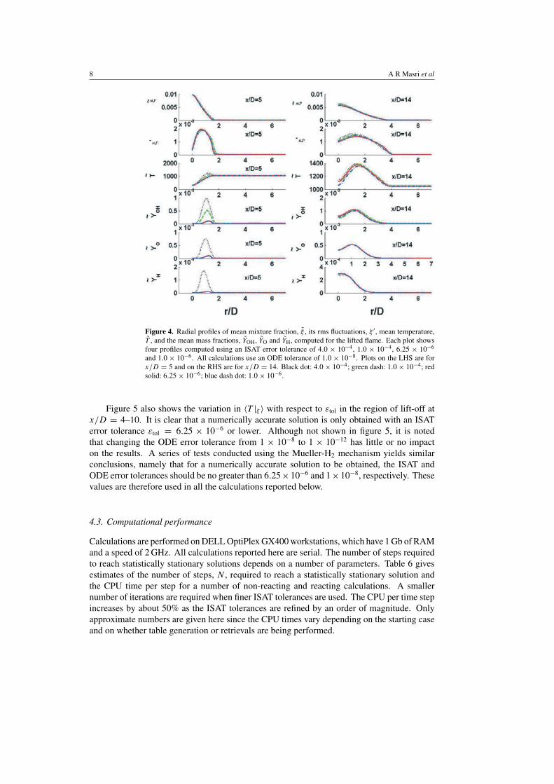
of 1 × 10−8, the following ISAT error tolerances are used: 4 × 10−4, 1 × 10−4, 2.5 × 10−5,6.25 × 10−6 and 1.0 × 10−6. In order to check the effects of the ODE error tolerance, anothercalculation was performed with an ISAT error of 6.25 × 10−6 and the ODE error tolerancedecreased from 1.0 × 10−8 to 1.0 × 10−12. The six cases investigated are summarized intable 5. The results of these tests are presented in figure 4, which shows radial profiles ofthe mean mixture fraction, ξ , and its rms fluctuations, ξ ′, mean temperature, T , and the meanmass fractions of OH, YOH, O, YO, and H, YH, computed at two axial locations, x/D = 5 andx/D = 14, in the flame. Each plot shows four profiles for cases 1, 2, 4 and 5 (listed in table 5),all of which are computed using the GRI21-H2 mechanism.

While the mean mixture fraction and its rms fluctuations are only slightly affected, it isclear that decreasing the ISAT error tolerance from 4×10−4 to 1×10−6 has a significant impacton the calculated temperature and compositional structure of the flame. While an ISAT errortolerance εtol = 4 × 10−4 is clearly unacceptable for these calculations, εtol = 6.25 × 10−6 isvery close to an accurate solution. This change in εtol has a direct impact on the lift-off heightas is clear form figure 5, which shows the conditional mean temperature at the stoichiometricmixture fraction, 〈T |ξs〉, calculated for the range of conditions detailed in table 5. At a givenaxial location, the conditional mean temperature, 〈T |ξs〉, is calculated as the ensemble averagetemperature of all particles whose mixture fraction, ξ , is in the range 0.45 < ξ < 0.5.

8 A R Masri et al

Figure 4. Radial profiles of mean mixture fraction, ξ , its rms fluctuations, ξ ′, mean temperature,T , and the mean mass fractions, YOH, YO and YH, computed for the lifted flame. Each plot showsfour profiles computed using an ISAT error tolerance of 4.0 × 10−4, 1.0 × 10−4, 6.25 × 10−6

and 1.0 × 10−6. All calculations use an ODE tolerance of 1.0 × 10−8. Plots on the LHS are forx/D = 5 and on the RHS are for x/D = 14. Black dot: 4.0 × 10−4; green dash: 1.0 × 10−4; redsolid: 6.25 × 10−6; blue dash dot: 1.0 × 10−6.

Figure 5 also shows the variation in 〈T |ξ 〉 with respect to εtol in the region of lift-off atx/D = 4–10. It is clear that a numerically accurate solution is only obtained with an ISATerror tolerance εtol = 6.25 × 10−6 or lower. Although not shown in figure 5, it is notedthat changing the ODE error tolerance from 1 × 10−8 to 1 × 10−12 has little or no impacton the results. A series of tests conducted using the Mueller-H2 mechanism yields similarconclusions, namely that for a numerically accurate solution to be obtained, the ISAT andODE error tolerances should be no greater than 6.25×10−6 and 1×10−8, respectively. Thesevalues are therefore used in all the calculations reported below.

4.3. Computational performance

Calculations are performed on DELL OptiPlex GX400 workstations, which have 1 Gb of RAMand a speed of 2 GHz. All calculations reported here are serial. The number of steps requiredto reach statistically stationary solutions depends on a number of parameters. Table 6 givesestimates of the number of steps, N , required to reach a statistically stationary solution andthe CPU time per step for a number of non-reacting and reacting calculations. A smallernumber of iterations are required when finer ISAT tolerances are used. The CPU per time stepincreases by about 50% as the ISAT tolerances are refined by an order of magnitude. Onlyapproximate numbers are given here since the CPU times vary depending on the starting caseand on whether table generation or retrievals are being performed.

PDF calculations of turbulent lifted flames of H2/N2 fuel 9

(a)

(b)

Figure 5. Calculated conditional mean temperature at the stoichiometric mixture fraction, 〈T |ξs〉,in the lifted flame. Plot (a) shows the computations versus x/D at ISAT error tolerances of4.0 × 10−4, 1.0 × 10−4, 2.5 × 10−5, 6.25 × 10−6 and 1.0 × 10−6. Plot (b) shows computationsat various x/D plotted against ISAT error tolerance. All calculations use an ODE error toleranceof 1.0 × 10−8.

Table 6. Computational requirements for a number of selected runs.

Particles Number ofMechanism Mesh per cell ISAT, εtol ODE, εtol steps, N CPU/step (s)

Non-reacting — Mesh 1 20 — — ∼1000 ∼2.5Non-reacting — Mesh 3 20 — — ∼3000 ∼26Reacting GRI21-H2 Mesh 2 20 1.0 × 10−4 1.0 × 10−8 ∼6000 ∼33Reacting GRI21-H2 Mesh 2 20 1.0 × 10−6 1.0 × 10−8 ∼3500 ∼65Reacting Mueller-H2 Mesh 3 20 1.0 × 10−4 1.0 × 10−8 ∼6000 ∼65Reacting Mueller-H2 Mesh 3 20 1.0 × 10−6 1.0 × 10−8 — ∼180

10 A R Masri et al

Figure 6. Measured and computed radial profiles of mean temperature, T , in the non-reactingjet. Symbols represent measurements. Five plots are shown for x/D = 1, 5, 10, 15 and 25. Thecomputations use mesh 3 and 20 particles per cell.

5. Results

The computations presented in this section use the fine mesh (mesh 3) with 20 particles percell. Mean quantities are obtained by averaging over 50 time steps. For the reacting case,an ISAT error tolerance of 6.25 × 10−6 is used with on ODE error tolerance of 1.0 × 10−8.Comparisons are made with the data of Cabra and co-workers [30, 31].

5.1. Non-reacting jet

Figure 6 shows radial profiles of the measured and computed temperatures at various axiallocations in the non-reacting jet. It should be noted here that the temperature is obtained fromthe computed density which linearly correlates with mixture fraction. The agreement betweenmeasurements and computations is reasonable, given the following qualifications: (i) the k–ε

model, with its standard constants, is known to over-predict the spreading rate of cylindricaljets. The standard adjustment of increasing one of the constants, Cε1, from 1.44 to 1.6, isnot effective here, and this is conjectured to be because of the lower density of the co-flow.Differences in density between the jet and the co-flow are known to affect the mixing behaviourof jets [38]. (ii) The disagreement between the measured and computed temperatures on thecentreline, particularly near the jet exit plane, is largely due to the fact the heat transfer fromthe hot co-flow is rather significant and yet not properly accounted for in the computations.Conjugate heat transfer between the jet and the co-flow is the subject of further investigationsand this aspect will be enhanced in the next generation of calculations.

PDF calculations of turbulent lifted flames of H2/N2 fuel 11

Figure 7. Measured and computed radial profiles of mean mixture fraction, ξ , and its rmsfluctuations, ξ ′, for the lifted flame. Plots on the LHS are for ξ and plots on the RHS are for ξ ′.Each column shows six plots for axial locations x/D = 1, 8, 10, 11, 14 and 26. The symbols ineach plot represent measurements, the solid line is computed using the GRI21-H2 mechanism andthe dotted line represents computations from the Mueller-H2 mechanism.

5.2. Lifted flame

Figures 7–10 show a comparison between measurements and computations at various axiallocations (x/D = 1, 8, 10, 11, 14, 26) in the lifted flame. Two scalars are presented ineach figure with: mean mixture fraction, ξ , and its rms fluctuations, ξ ′, in figure 7; meantemperature, T , and its rms fluctuations, T ′, presented in figure 8; the mean mass fractions ofhydrogen, YH2 , and hydroxyl, YOH, in figure 9; and the mean mass fractions of water, YH2O, andoxygen, YO2 , in figure 10. Results are presented for both the Mueller-H2 and GRI21-H2

mechanisms.Figure 7 shows that the measured and computed mixing fields are in good agreement at

upstream locations but start to deviate at x/D � 11, with the computations under-predictingξ and over-predicting the spreading rate of the jet. It should be noted here that increasingthe constant Cε1 from 1.44 to 1.6 does not remedy this deficiency as is normally the casefor turbulent jets. This is probably because the jet is issuing in heated air where the densityis less than that of the jet fluid. The rms fluctuations of mixture fraction, ξ ′, are generallyover-predicted right across the jet length. This may be overcome by increasing the mixing-model constant, Cφ, and this aspect is discussed later. These results are consistent for boththe Mueller-H2 and GRI21-H2 mechanisms.

The mean temperature profiles (shown in figure 8) indicate that the lift-off heightscomputed using the Mueller-H2 and GRI21-H2 mechanisms are very different and bracket theexperimental lift-off height, which occurs at about 11 jet diameters as seen from the measuredrise in peak temperature. The computed lift-off heights for the GRI21-H2 and Mueller-H2

12 A R Masri et al

Figure 8. Measured and computed radial profiles of mean temperature, T , and its rms fluctuations,T ′, for the lifted flame. Plots on the LHS are for T and plots on the RHS are for T ′. Each columnshows six plots for axial locations x/D = 1, 8, 10, 11, 14 and 26. The symbols in each plotrepresent measurements, the solid line is computed using the GRI21-H2 mechanism and the dottedline represents computations from the Mueller-H2 mechanism.

mechanisms are x/D ∼ 8 and 14, respectively. The GRI21-H2 mechanism results in higherrms fluctuations of temperature, especially at upstream locations. However, the computedprofiles of T ′ using the Mueller-H2 mechanism are very close to the measurements.

The mean species mass fractions (shown in figures 9 and 10) confirm the results shownearlier for temperature, namely, that the computations using the Mueller-H2 and GRI21-H2

mechanisms, generally bracket the experimental results at least for the upstream measurementlocations. This is true for the mass fractions of H2, H2O, O2 and OH shown in figures 9 and10. Further downstream at x/D = 26, the peak mass fraction of OH is under-predicted byboth mechanisms while the computed profiles of H2, H2O and O2 are adequate except for adiscrepancy in the spreading rate that is mainly due to the turbulence model.

Axial profiles of the computed mean temperature and mean mass fractions of OH, O and Hare plotted in figure 11 for both Mueller-H2 and GRI21-H2 mechanisms and for radial locationsr/D = 0, 0.5, 1.0 and 1.5, which span the base of the flame. The measured mean centrelinetemperatures and mass fractions of OH are also shown on the relevant plots. A sharper rise intemperature is observed with the GRI21-H2 mechanism, and lift-off is first observed at a radiallocation of about r/D = 1. This is also observed in the axial profiles for YOH, YO and YH,which show an increase starting to occur at r/D = 1.0 as early as x/D = 5. The peak meanmass fraction of oxygen, YO, occurs first at x/D = 8 and this may be taken as the computedlocation of the flame base. With the Mueller-H2 mechanism, the profiles of temperature andspecies mass fractions overlap regardless of the radial locations, implying that lift-off occurscloser to the jet centreline. Gauging by the peak location of species mass fractions, lift-offoccurs at about x/D = 18, which is further from measurements.

PDF calculations of turbulent lifted flames of H2/N2 fuel 13

Figure 9. Measured and computed radial profiles of mean mass fractions of H2 and OH, YH2 andYOH, for the lifted flame. Plots on the LHS are for YH2 and plots on the RHS are for YOH. Eachcolumn shows six plots for axial locations x/D = 1, 8, 10, 11, 14 and 26. The symbols in eachplot represent measurements, the solid line is computed using the GRI21-H2 mechanism and thedotted line represents computations from the Mueller-H2 mechanism.

Figure 10. Measured and computed radial profiles of mean mass fractions of H2O and O2, YH2O

and YO2 , for the lifted flame. Plots on the LHS are for YH2O and plots on the RHS are for YO2 .Each column shows six plots for axial locations x/D = 1, 8, 10, 11, 14 and 26. The symbols ineach plot represent measurements, the solid line is computed using the GRI21-H2 mechanism andthe dotted line represents computations from the Mueller-H2 mechanism.

14 A R Masri et al

Figure 11. Axial profiles of mean temperature, T , and the mean mass fractions YOH, YO and YHcomputed for the lifted flame. Plots on the LHS are computed using GRI21-H2 mechanism andplots on the RHS are computed using the Mueller-H2 mechanism. Each plots shows four profilesfor r/D = 0, 0.5, 1.0 and 1.5. Symbols are measurements for r/D = 0. Red solid: r/D = 0.0;black dot: r/D = 0.5; green dash: r/D = 1.0; cyan dash dot: r/D = 1.5.

Measured and computed scatter plots of temperature and the mass fraction of OH areshown in figure 12 for various axial locations in the flame. All the data points or fluid samplescorresponding to the particular axial location are shown. The computations are obtainedusing the GRI21-H2 mechanism, and these agree qualitatively well with the measurements. Atx/D = 8, the domain below the fully burnt limit is similarly populated, indicating the existenceof fluid samples that are partially burnt and in the process on igniting. This proportion increasesat x/D = 11, indicating intense auto-ignition that is almost complete at x/D = 14, wheremost of the data points lie closer to the fully burnt limits.

6. Modelling issues

The hybrid approach adopted in this paper involves a turbulence model, a mixing model and achemistry model. The turbulence model used here is rather simple and not elaborated furtherin this paper except for re-stating that changing the constant Cε1 from 1.44 to 1.6 has become astandard approach that will improve the k–ε calculation of the jet spreading rate. However, thisimprovement did not occur in the current geometry possibly because the co-flowing mixturein which the jet issues is heated and hence the mixing rates in the jet are affected by thesignificant density ratio between the jet and the co-flow [38]. The discussion that follows isonly concerned with modelling of mixing and chemical reactions.

6.1. Effects of Cφ

The MC mixing model used here is also rather simple. Other mixing models that may be used inthe future are the IEM and the Euclidean minimum spanning tree (EMST) models [39]. More

PDF calculations of turbulent lifted flames of H2/N2 fuel 15

Figure 12. Measured (LHS) and computed (RHS) scatter plots for temperature and the mass fractionof OH, YOH, against mixture fraction, ξ , plotted for x/D = 8, 11 and 14. The computations arefor the GRI21-H2 mechanism.

sophisticated mixing models are currently being developed by Klimenko and Pope [40]. Theconstant Cφ used with the MC model is changed from Cφ = 2.0, which is the standard value,to Cφ = 2.3 (assumed by Lindstedt and Louloudi [16]) and 20, respectively. Figure 13 showsradial profiles of mean mixture fraction, ξ , and its rms fluctuations, ξ ′, mean temperature, T ,and its rms fluctuations, T ′, and the mean mass fractions of OH, YOH, and O, YO, computedat two axial locations, x/D = 5 and x/D = 14, in the flame. Each plot shows three profilescomputed for Cφ = 2.0, 2.3 and 20. The following points are worth noting.

• IncreasingCφ from 2.0 to 2.3 has little impact on the mixing: the rms fluctuations of mixtureremain over-predicted as shown earlier. It is worth mentioning here that Cφ = 2.3 wasfound to be the optimal value in the calculations of Lindstedt and Louloudi [16].

• As expected, increasing Cφ from 2.0 to 20 reduces the rms fluctuations significantly andenhances mixing as shown from the profiles of ξ ′ and T ′. Although the flame lift-off heightdecreases slightly from about eight to six diameters, the flame remains lifted indicatingthat the lift-off height is affected by the rates of both mixing and chemical reactions. Thisdependence on the chemical kinetics confirms the auto-ignition characteristics of this jetflame.

6.2. Effects of reaction rates

In order to understand the impact of the reaction rates on auto-ignition, a simple sensitivityanalysis has been conducted of both mechanisms using an idealized model problem. A simpleone-dimensional channel is set-up (essentially a plug-flow reactor) with a lean but reactivemixture issuing from one end at a velocity of 100 m s−1. The fluid entering the channel hasthe following composition: mixture fraction ξ = 0.05, temperature = 1003.03 K and massfractions YH2 = 0.001 171 29, YO2 = 0.162 326, YH2O = 0.061 319 1. This mixture lies alongthe mixing line formed by the jet and pilot fluid in the flame considered in this paper.

16 A R Masri et al

Figure 13. Radial profiles of mean mixture fraction, ξ , its rms fluctuations, ξ ′, mean temperature,T , its rms fluctuations, T ′, and the mean mass fraction of OH and O, YOH and YO, computed forthe lifted flame. Each plot shows three profiles for Cφ = 2.0, 2.3 and 20. Plots on the LHS are forx/D = 5 and on the RHS are for x/D = 14. Red solid: Cφ = 2.0; black dot: Cφ = 2.3; greendash: Cφ = 20.

Using the GRI21-H2 mechanism, the mixture auto-ignites at some x = 125 mm within thechannel, giving a peak temperature of 1118.1 K. Consistent with the turbulent flame results,auto-ignition for the Mueller-H2 mechanism occurs later at x = 200 mm. In order to testthe impact of individual reactions on auto-ignition, the rate of each reaction is changedseparately (by doubling the pre-exponential factor, A) and the computations repeated for thesame condition. It is found that some reactions speed-up the auto-ignition process while otherscause a delay. The three most dominant reactions that cause a delay or speed-up in auto-ignitionare listed for both mechanisms in table 7.

Computations of the lifted flames are now repeated with a modified mechanism where therate of the reaction that dominates the speed-up of auto-ignition: O2 +H ↔ O+OH is doubled.This is reaction 11 in the GRI21-H2 mechanism and reaction 1 in the Mueller-H2 mechanism.The results are summarized in figures 14 and 15, which show the change in composition andlift-off height due to the rate increase.

Figure 14 shows plots of mean temperature, T , and mean mass fractions of OH, Oand H at various axial locations in the flame computed using the standard and modifiedGRI21-H2 mechanisms. Figure 15 shows similar plots computed using the standard andmodified Mueller-H2 mechanisms. The following points are worth noting.

• As expected, and consistent with the simple channel calculations, auto-ignition occursearlier and the flame base shifts upstream. Using the computed peak mean mass fractionof oxygen radical as an indicator, the lift-off height of the turbulent flame shifts fromx/D = 8 to x/D = 5 for the GRI21-H2 mechanism and from x/D = 18 to x/D = 9 forthe Mueller-H2 mechanism.

• The peak species mass fractions also change significantly.

PDF calculations of turbulent lifted flames of H2/N2 fuel 17

Table 7. Reactions from GRI21-H2 and Mueller-H2 mechanisms to which auto-ignition is mostsensitive.

GRI21-H2 Mueller-H2

Reaction Reactionnumber Reaction number Reaction

Increasing rate delays auto-ignition8 H + O2 + H2O ↔ HO2 + H2O 13 HO2 + OH ↔ H2O + O2

9 H + O2 + N2 ↔ HO2 + N2 12 HO2 + O ↔ O2 + OH7 H + O2 + O2 ↔ HO2 + O2 10 HO2 + H ↔ H2 + O2

Increasing rate speeds up auto-ignition11 O2 + H ↔ O + OH 1 O2 + H ↔ O + OH

3 O + H2 ↔ H + OH 2 O + H2 ↔ H + OH21 H2 + OH ↔ H2O + H 3 H2 + OH ↔ H2O + H

Figure 14. Radial profiles of mean temperature, T , and the mean mass fractions YOH, YO and YHcomputed using the GRI21-H2 mechanism at three axial locations in the lifted flame, x/D = 5, 10and 14. Each plot shows two profiles, one for the standard mechanism and the other obtained whenthe rate of reaction 11 is doubled by doubling the pre-exponential factor A. Red solid: standard;black dot: doubled.

• These calculations confirm that the chemical kinetics is very important in controlling theearly regions of the turbulent flames studied here. The lift-off height is affected by ratesof both mixing and chemical reactions, with there being a marked sensitivity to the ratesof the controlling reactions.

7. Discussion

It is clear from the figures presented earlier, especially figure 13, that this flame, althoughstill affected by mixing, is largely controlled by chemical processes. The dependence on thechemical kinetic mechanism is clear, and further investigations are needed to confirm as towhich mechanism (and kinetic rates) would be more relevant for the modelling of hydrogen

18 A R Masri et al

Figure 15. Radial profiles of mean temperature, T , and the mean mass fractions YOH, YO and YHcomputed using the Mueller-H2 mechanism at three axial locations in the lifted flame, x/D = 5, 10and 14. Each plot shows two profiles, one for the standard mechanism and the other obtained whenthe rate of reaction 1 is doubled by doubling the pre-exponential factor A. Red solid: standard;black dot: doubled.

auto-ignition. What is clear from the calculations presented here is that the GRI21-H2 andMueller-H2 mechanisms straddle the data and the rates of some individual reactions have ahuge impact on the lift-off height as well as the flame composition.

A conclusive statement as to the presence of auto-ignition or flame propagation processesat the flame base cannot be made here. Experimentally, the flame is very sensitive to thetemperature in the co-flowing pilot and changes, at least qualitatively, from a quietly liftedflame to a noisy flame with larger fluctuations at the base as the pilot temperature decreases.It is not clear whether this implies a definite transition from auto-ignition to premixed flamepropagation, or simply a co-existence of both processes. This issue is clearly of importanceand warrants further investigation.

Proceeding with the view that auto-ignition does indeed take place, an important questionto address here is which mixture fraction range is most responsible for auto-ignition. This is aninteresting issue that is explored a little further in this section. The excess temperature, Texcess,conditional on mixture fraction is plotted versus axial location is figure 16 for calculations usingboth the GRI21-H2 and Mueller-H2 mechanisms. The excess temperature is representative ofthe heat release and is defined as Texcess = T –Tmixing, where T is the computed temperatureand Tmixing is the mixing temperature at the mixture fraction of the fluid sample. Three mixturefraction bands are shown in the three plots presented here: 0 < ξ < 0.1, 0.1 < ξ < 0.2 and0.2 < ξ < 0.3. It is seen that fluid samples in the mixture fraction range 0 < ξ < 0.1 ignite atearlier axial locations than richer mixtures. This is expected since hot co-flowing gases fromthe pilot will first mix with enough jet fuel to produce lean mixtures that are hot and hencehave short ignition delays. Richer mixtures will have lower temperatures and hence longerignition delays.

PDF calculations of turbulent lifted flames of H2/N2 fuel 19

Figure 16. Scatter plots of the excess temperature, Texcess = T –Tmixing, conditional with respectto mixture fraction and plotted versus axial location. Three plots are presented for three mixturefraction bands with ranges (from top to bottom) 0 < ξ < 0.1, 0.1 < ξ < 0.2 and 0.2 < ξ < 0.3.

This finding is consistent with separate calculations made using the simple channel flowproblem discussed earlier. It is also consistent with the reported findings from DNS studies[24–28]. Fluid samples in the mixture fraction range 0 < ξ < 0.1 have the fastest ignitionrate and this is controlled purely by chemical kinetics rather than mixing. These conclusionsapply for both the GRI21-H2 and Mueller-H2 mechanisms.

8. Conclusions

The hybrid RANS–PDF (composition) approach is used here to compute successfully thestructure of lifted flames issuing in a vitiated co-flow. Two chemical kinetic mechanisms are

20 A R Masri et al

implemented using the ISAT approach. Numerically accurate solutions are obtained after asignificant testing for grid convergence, number of particles per cell and error tolerancesassociated with the ISAT approach.

It is found that, although mixing rates are still important, the flame is largely controlledby the chemical kinetics and the mechanisms used give lift-off heights that straddle theexperimental data. The computed mean temperatures and species mass fractions also comparefavourably with experimental data. At downstream locations, the flow and mixing fields deviatefurther from experiments in line with what is expected for the k–ε model.

The lift-off height and flame composition at the stabilization base are extremely sensitiveto the rates of some individual reactions, hence stressing the importance of chemical kineticsin this flow configuration. For the fuel mixture used here, it is found that the shortest ignitiondelays are obtained for lean mixtures spanning the mixture fraction range 0.0 < ξ < 0.1.

Acknowledgments

This work is supported by the Australian Research Council and the US Air Force Office ofScientific Research grant no F49620-00-1-0171. The authors are also grateful for the supportof the University of Sydney and Cornell University.

Appendix

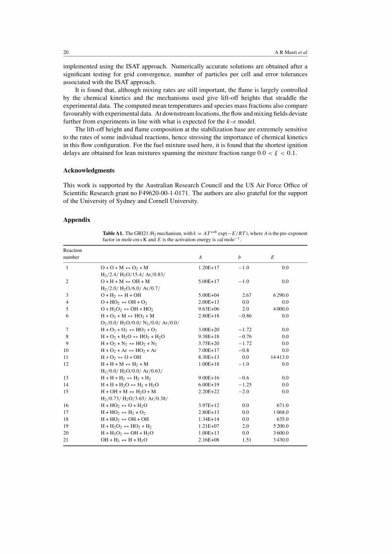
Table A1. The GRI21-H2 mechanism, with k = AT ∗∗b exp(−E/RT ), where A is the pre-exponentfactor in mole cm s K and E is the activation energy is cal mole−1.

Reactionnumber A b E

1 O + O + M ↔ O2 + M 1.20E+17 −1.0 0.0H2/2.4/ H2O/15.4/ Ar/0.83/

2 O + H + M ↔ OH + M 5.00E+17 −1.0 0.0H2/2.0/ H2O/6.0/ Ar/0.7/

3 O + H2 ↔ H + OH 5.00E+04 2.67 6 290.04 O + HO2 ↔ OH + O2 2.00E+13 0.0 0.05 O + H2O2 ↔ OH + HO2 9.63E+06 2.0 4 000.06 H + O2 + M ↔ HO2 + M 2.80E+18 −0.86 0.0

O2/0.0/ H2O/0.0/ N2/0.0/ Ar/0.0/

7 H + O2 + O2 ↔ HO2 + O2 3.00E+20 −1.72 0.08 H + O2 + H2O ↔ HO2 + H2O 9.38E+18 −0.76 0.09 H + O2 + N2 ↔ HO2 + N2 3.75E+20 −1.72 0.0

10 H + O2 + Ar ↔ HO2 + Ar 7.00E+17 −0.8 0.011 H + O2 ↔ O + OH 8.30E+13 0.0 14 413.012 H + H + M ↔ H2 + M 1.00E+18 −1.0 0.0

H2/0.0/ H2O/0.0/ Ar/0.63/

13 H + H + H2 ↔ H2 + H2 9.00E+16 −0.6 0.014 H + H + H2O ↔ H2 + H2O 6.00E+19 −1.25 0.015 H + OH + M ↔ H2O + M 2.20E+22 −2.0 0.0

H2/0.73/ H2O/3.65/ Ar/0.38/

16 H + HO2 ↔ O + H2O 3.97E+12 0.0 671.017 H + HO2 ↔ H2 + O2 2.80E+13 0.0 1 068.018 H + HO2 ↔ OH + OH 1.34E+14 0.0 635.019 H + H2O2 ↔ HO2 + H2 1.21E+07 2.0 5 200.020 H + H2O2 ↔ OH + H2O 1.00E+13 0.0 3 600.021 OH + H2 ↔ H + H2O 2.16E+08 1.51 3 430.0

PDF calculations of turbulent lifted flames of H2/N2 fuel 21

Table A1. (Continued.)

ReactionNumber A b E

22 OH + OH(+M) ↔ H2O2(+M) 7.40E+13 −0.37 0.0LOW/2.3E+18 −0.9 −1.7E+3TROE/0.7346 94.0 1756.0 5182.0/

H2/2.0/ H2O/6.0/ Ar/0.7/

23 OH + OH ↔ O + H2O 3.57E+04 2.4 −2 110.024 OH + HO2 ↔ H2O + O2 2.90E+13 0.0 −500.025 H + H2O2 ↔ HO2 + H2O 1.75E+12 0.0 320.026 H + H2O2 ↔ HO2 + H2O 5.80E+14 0.0 9 560.027 HO2 + HO2 ↔ O2 + H2O2 1.30E+11 0.0 −1 630.028 HO2 + HO2 ↔ O2 + H2O2 4.20E+14 0.0 12 000.0

Table A2. The Mueller-H2 mechanism, with k = AT ∗∗b exp(−E/RT ), where A is the pre-exponent factor in mole cm s K and E is the activation energy is cal mole−1.

Reactionnumber A b E

1 H + O2 ↔ O + OH 1.915E+14 0.0 16 439.02 O + H2 ↔ H + OH 0.508E+05 2.67 6 290.03 H2 + OH ↔ H2O + H 0.216E+09 1.51 3 430.04 O + H2O ↔ OH + OH 2.970E+06 2.02 13 400.05 H2 + M ↔ H + H + M 4.577E+19 −1.40 104 380.0

H2/2.5/ H2O/12/

6 O + O + M ↔ O2 + M 6.165E+15 −0.50 0.0H2/2.5/ H2O/12/

7 O + H + M ↔ OH + M 4.714E+18 −1.00 0.08 H + OH + M ↔ H2O + M 2.212E+22 −2.00 0.0

H2/2.5/ H2O/6.3/

9 H + O2(+M) ↔ HO2(+M) 1.475E+12 0.60 0.0LOW/3.482E+16 −0.411 −1.115E+3TROE/0.5 1E−30 1E+30/

H2/2.5/ H2O/12/10 HO2 + H ↔ H2 + O2 1.66E+13 0.0 823.011 HO2 + H ↔ OH + OH 7.079E+13 0.0 295.012 HO2 + O ↔ O2 + OH 0.325E+14 0.0 0.013 HO2 + OH ↔ H2O + O2 2.890E+13 0.0 −497.014 HO2 + HO2 ↔ H2O2 + O2 4.200E+14 0.0 11 982.015 HO2 + HO2 ↔ H2O2 + O2 1.300E+11 0.0 −1 629.016 H2O2(+M) ↔ OH + OH(+M) 2.951E+14 0.0 48 430.0

LOW/1.202E+170.0 + 4.55E+4TROE/0.5 1E−30 1E+30/

H2/2.5/ H2O/12/

17 H2O2 + H ↔ H2O + OH 0.241E+14 0.0 3 970.018 H2O2 + H ↔ HO2 + H2 0.482E+14 0.0 7 950.019 H2O2 + O ↔ OH + HO2 9.550E+06 2.0 3 970.020 H2O2 + OH ↔ HO2 + H2O 1.000E+12 0.0 0.021 H2O2 + OH ↔ HO2 + H2O 5.800E+14 0.0 9 557.0

References

[1] Vanquickenborne L and Van Tiggelen A 1996 Combust. Flame 10 59–69[2] Broadwell J E, Dahm W J A and Mungal M G 1984 Proc. Combust. Inst. 20 303–10

22 A R Masri et al

[3] Pitts W M 1990 Proc. Combust. Inst. 23 661–8[4] Pitts W M 1988 Proc. Combust. Inst. 22 809–16[5] Kalghatgi G T 1984 Combust. Sci. Technol. 41 17–29

Kalghatgi G T 1981 Combust. Sci. Technol. 26 233–9[6] Eickhoff H, Lenze B and Leuckel W 1984 Proc. Combust. Inst. 20 311–8[7] Gollahalli S R, Savas O, Huang R F and Rodriquez Azara J L 1986 Proc. Combust. Inst. 21 1463–71[8] Takahashi F and Schmoll W J 1990 Proc. Combust. Inst. 23 677–83[9] Peters N and Williams F A 1983 AIAA J. 21 423–9

[10] Schefer R W, Namazian M and Kelly J 1990 Proc. Combust. Inst. 23 669–76[11] Kelman J B and Masri A R 1998 Combust. Sci. Technol. 135 117–34[12] Tacke M M, Geyer D, Hassel E P and Janicka J 1998 Proc. Combust. Inst. 27 1157–65[13] Upatnieks A, Driscoll J F and Ceccio S L 2002 Proc. Combust. Inst. 29 1897–903[14] Tang Q, Xu J and Pope S B 2000 Proc. Combust. Inst. 28 133–40[15] Lindstedt R P, Louloudi S A and Vaos E M 2000 Proc. Combust. Inst. 28 149–56[16] Lindstedt R P and Louloudi S A 2002 Proc. Combust. Inst. 29 2147–54[17] Liu K, Pope S B and Caughey D A 2003 Calculations of a turbulent bluff-body stabilized flame 3rd Joint Meeting

of the US Sections of the Combustion Institute (Chicago, March 2003)[18] Klimenko A Yu 1990 Fluid Dyn. 25 327–34[19] Bilger R W 1993 Phys. Fluids A 5 436–44[20] Kim S H, Huh K Y and Bilger R W 2002 Proc. Combust. Inst. 29 2131–7[21] Pitsch H 2002 Proc. Combust. Inst. 29 2679–85[22] Mastorakos E T A, Baritaud B and Poinsot T J 1997 Combust. Flame 109 198–223[23] Mastorakos E T A, da Cruz T A, Baritaud B and Poinsot T J 1997 Combust. Sci. Technol. 125 243–82[24] Sreedhara H and Lakshmisha K N 2000 Proc. Combust. Inst. 28 25–34[25] Sreedhara H and Lakshmisha K N 2002 Proc. Combust. Inst. 29 2051–9[26] Sreedhara H and Lakshmisha K N 2002 Proc. Combust. Inst. 29 2069–77[27] Hilbert R and Thevenin D 2002 Combust. Flame 128 22–37[28] Hilbert R, Tap F, Veynante D and Thevenin D 2002 Proc. Combust. Inst. 29 2079–85[29] Dally B B, Karpetis A N and Barlow R S 2002 Proc. Combust. Inst. 29 1147–54[30] Cabra R, Myrvold T, Chen J Y, Dibble R W, Karpetis A N and Barlow R S 2002 Proc. Combust. Inst. 29 1881–8[31] Cabra R, http://www.me.berkeley.edu/cal/VCB/[32] Pope S B 1997 Combust. Theory Modelling 1 1–24[33] Mueller M A, Kim T J, Yetter R A and Dryer F L 1999 Flow reactor studies and kinetic modeling of the H2/O2

reaction Int. J. Chem. Kinetics 31 113–25[34] Bowman C T, Hanson R K, Davidson D F, Gardiner Jr, Lissianski V, Smith G P, Golden D M, Goldenberg M

and Frenklach M 1999 Gri-Mech 2.11 http://www.me.berkeley.edu/gri mech/[35] Kreutz T G and Law C K 1996 Combust. Flame 104 157–75[36] Im H G, Chen J H and Law C K 1998 Proc. Combust. Inst. 27 1047–56[37] Maas U and Warnatz J 1988 Proc. Combust. Inst. 22 1695–704[38] Pitts W M 1991 Exp. Fluids 11 125–34

Pitts W M 1991 Exp. Fluids 11 135–41[39] Subramanian S and Pope S B 1998 Combust. Flame 115 487–514[40] Klimenko A Yu and Pope S B 2003 Phys. Fluids 15 1907–25