Single-frequency GNSS retrieval of vertical total electron content

(VTEC) with GPS L1 and Galileo E5 measurements

Torben Schuler1,2,*, and Olushola Abel Oladipo3,4

1 University of the Federal Armed Forces Munich, Faculty of Aerospace Engineering, Department LRT9.2, 85577 Neubiberg,Germany*Corresponding author: e-mail: dr_schueler@gmx.net

2 Geodetic Observatory Wettzell, Federal Agency of Cartography and Mapping (BKG), Sackenrieder Str. 25, 93444 Bad Kotzting,Germany

3 University of Ilorin, Physics Department, P.M.B., 1515 Ilorin, Nigeria4 Alexander von Humboldt Research Fellow at University of the Federal Armed Forces Munich, Germany

Received 27 February 2012 / Accepted 13 February 2013

ABSTRACT

The European Galileo satellite navigation system offers a signal in space that will enable us to deduce range measurements ofunprecedented precision: the E5 broadband signal. These new code range measurements would be up to three or four times moreaccurate compared to nowadays GPS L1. However, E5 will be the only Galileo signal of that outstanding performance. For thisreason, a single-frequency single-site ionospheric delay estimator is experimented with to retrieve absolute VTEC data. A single-frequency VTEC retrieval algorithm was developed and tested. It is following the principles published in Xia (1992), Issler et al.(2004), and Leick (1995, 2004). During the validation phase, we devoted considerable time to process GPS L1 measurements inorder to assess the level of precision obtainable with current real-world GNSS measurements. We found the global average RMS tobe close to 4 TECU (1.5–2.5 TECU at mid- and higher latitude stations) what is considered to be a promising result. The verylimited Galileo satellite constellation present during the time of this study did not allow us to run the absolute VTEC retrieval algo-rithm with real Galileo data. However, we can demonstrate the significant improvements related to the Galileo E5 signal with thehelp of satellite-specific ionosphere retrieval results from the Galileo experimental satellite GIOVE-B, although only a limited setof data was available for that purpose. In addition, we are presenting a test case based on simulated data that also underlines that theprecision figures will clearly improve when using Galileo E5 data. This could make single-frequency ionosphere retrieval moreattractive in the future.

Key words. vertical total electron content (VTEC) – GPS – Galileo – GNSS – E5 wideband signal – ionosphere monitoring

1. Introduction

One method to separate the ionospheric delay from all the othercomponents inherent in GNSS measurements is to exploit thecharacteristics of group versus phase delay. In fact, the iono-spheric delay has opposite signs on both the code range(‘‘pseudoranges’’) and carrier phase measurements.

Although not in widespread use today, a single-frequencyGNSS receiver can actually be useful for sensing ionosphericdelays, too. A least-squares block adjustment procedure is usedfor this purpose. A sequential filter implementation of this algo-rithm, which is not in the focus of this paper, could be used forreal-time ionosphere monitoring.

1.1. Importance of code ranges

The single-frequency approach makes use of a linear combina-tion of code range and carrier phase measurements. Coderanges are less accurate than carrier phase measurements, inparticular because multipath effects impact ranges to a largerextent than carrier phases, but there are variations for the differ-ent GNSS signals depending on design parameters such as sig-nal structure and bandwidth (Eissfeller et al. 2007). Inparticular, the E5 AltBOC-modulated broadband signal of thefuture Galileo navigation satellite system will feature an out-

standing multipath performance that can be three or even fourtimes lower compared to the current signals such as GPS L1.The increased multipath resistance and reduced code noiseare a result of both the AltBOC(15,10) modulation applied tothis signal and the enhanced bandwidth of more than 50 MHzcompared to 24 MHz of the GPS L1 signal in space. This factcan make the single-frequency approach more competitivecompared to dual-frequency methods, although receiver perfor-mance has evolved during the past too, so that GPS L1 data canalso be successfully processed as demonstrated in this paper.

1.2. Literature review

The idea to use single-frequency GPS measurements for iono-spheric delay estimation is not new, but literature on this topic islimited, mainly because of the code noise problem outlinedbefore that has delayed the realization of this conceptsignificantly.

Yuan & Ou (2001) outline the basic methodology, but theauthors only recognize the relative character of the code-minus-carrier approach rather than the possibility to determineabsolute total electron content.

Coco et al. (1991) published an article focusing on theestimation of differential instrumental delay biases to make

J. Space Weather Space Clim. 3 (2013) A11DOI: 10.1051/swsc/2013033� T. Schuler et al., Published by EDP Sciences 2013

OPEN ACCESSRESEARCH ARTICLE

This is an Open Access article distributed under the terms of the Creative Commons Attribution License (http://creativecommons.org/licenses/by/2.0),which permits unrestricted use, distribution, and reproduction in any medium, provided the original work is properly cited.

the estimation of total electron content from dual-frequencyGPS measurements feasible. This comprises, in particular, theestimation of the L2-L1 differential group delay. Although acalibration technique is depicted, the horizontal interpolationapproach carried out for the total electron content is similar tothe one followed in this note.

Xia (1992) describes an experiment to retrieve absolute ion-ospheric delay errors from a single-frequency GPS receiver.This approach published in 1992 underlines that the use of acode range minus carrier phase combination (CMC) enablesus to determine the total electron content from data collectedon just one instead of both GPS frequencies, although somedetails necessary for a successful delay retrieval are not com-pletely clear, and the author admits that this study is just a veryfirst step and a demonstration of the technique. Just at the sameconference, Cohen et al. (1992) present a paper of similar con-tents. A first-order spherical harmonics model is chosen for hor-izontal interpolation of the ionospheric delays at the piercepoints, which are expressed in a sun-fixed reference frame. Acouple of years later, Lestarquit et al. (1996) depict a sequentialfilter algorithm for L1 only ionospheric delay estimation, whichis also mentioned by Issler et al. (2004). Finally, a more recentpublication by Mayer et al. (2008) is – in essence – of the samecontents.

2. Description of algorithm

As already mentioned, the method of single-frequency site-spe-cific VTEC retrieval is not new, so that only a brief descriptionis given here. The reader may refer to the literature cited in thepreceding section. In particular, we refer to Leick (1995, 2004)who outlines this method, although its application is focusingon position accuracy improvement rather than ionosphere mon-itoring in his textbook.

The appropriate observable containing the ionosphericdelay in slant direction is the code-minus-carrier observationthat eliminates all geometry-dependent components with theimpact of the ionospheric propagation delay being the promi-nent remainder in the observation equation:

CMCi ¼ PRi � k� /i ¼ 2mi �Cf 2� VTECi þ b;

b ¼ Ni � kþ bi þ bREC þ bCh; ð1Þwhere

CMC Code-minus-carrier observable containing theionospheric delay (m)

PR Code range measurement (‘‘pseudo range’’) (m)k Carrier wave wavelength (m)/ Carrier phase measurement (cycles)m Mapping function to project slant to zenith direction (/)C Constant; C � 40.309 · 1016 according to Petit &

Luzum (2010)f Carrier wave frequency (Hz)VTEC Vertical total electron content (TECU)b Bias term (combined term)N Ambiguity term (cycles)bi Satellite-specific biasbREC Receiver common biasbCH Receiver interchannel bias

Our target parameter is VTEC that is to be estimated from aset of CMC observables to various GNSS satellites. It should benoted that VTECi differs for each satellite i, because the rays arepassing through different parts of the ionosphere, and a numberof bias terms are to be determined. As a matter of fact, thissystem of equations cannot be solved ad hoc, because it isunderdetermined. A common method to solve this problem isto use a horizontal interpolation function, a low-order polyno-mial in our case with three to four parameters, and to determineits coefficients rather than each piercepoint-related VTECi indi-vidually. The variations in time domain are modeled as piece-wise linear function. The system of equations is then solvedusing a least-squares block adjustment procedure.

2.1. Biases

A bias problem is present and must be addressed. The sum ofall biases is denoted as b here. The satellite-receiver-specificambiguity terms are important bias terms in addition to thesatellite-specific bias bi. The ambiguities change as soon as a(non-fixable) cycle slip occurs. Such phase jumps are usuallyrelated to obstacles hiding the satellite signal, strong multipatheffects and ionospheric scintillations. The receiver-specific biasis considered to be common to all observations. In addition, wetake an interchannel bias into consideration: Nowadays receiv-ers use a number of hardware channels for satellite tracking.Each of these channels may exhibit an individual delay. Thesedelays are supposed to be estimated in a geodetic-grade recei-ver, e.g., by tracking one selected satellite on all hardwarechannels, but our algorithm is also supposed to work withmass-market receivers which are very cheap and for whichwe cannot assume that such receiver-internal calibration proce-dures will be carried out with sufficient accuracy. However,please note that mass-market receivers might be equipped withless stable tracking loops and thus are more susceptible to lossof lock causing more cycle slips than high-quality receivers.

We effectively estimate the complete b terms for each unin-terrupted satellite arc (typically between 150 and 180 min usinga 20� elevation mask). Our assumption is that the bias termdoes not change over that (relatively short) period of time.We do not separate the common bias bREC from the rest ofthe terms in our implementation.

2.2. Mapping function

The slant ionospheric propagation delays are separated from thebias terms with the help of a mapping function that relates theslant delay to the vertical direction. A commonly used approx-imation called ‘‘single-layer model’’ of the ionosphere isadopted, see e.g., Hoffmann-Wellenhof et al. (1993). The preci-sion of this mapping function is critical from our experience,even when using an elevation cut-off of 20�. For this reason,station-specific effective heights were adopted and a modifiedmapping function is used that is documented in Dach et al.(2007). We can confirm their global effective ionosphere heightof 450 km, but considerable variations can be stated, predomi-nantly in the North-South direction. We are using a fixed heightfor each site: the median from a daily analysis of annual datasets. Smaller seasonal variations exist for certain stations, diur-nal variations can be present but have not been investigated yet.An alternative method using the NeQuick2 ray-tracer (Navaet al. 2008) to derive precise obliquity factors is underway.

J. Space Weather Space Clim. 3 (2013) A11

A11-p2

3. GPS IGS LEO network test

The year 2003 appears to be a proper time period to test the sin-gle-frequency ionosphere monitoring approach with real-worldGPS data. Intentionally not right in the middle of the solarcycle’s maximum activity nor located in its minimum, it is stilla period of slightly higher activity than what we would call‘‘typical’’. Moreover, the already-mentioned October 2003 ion-osphere storm (Doherty et al. 2004) provides a prominent sig-nature in the data sets of most stations.

3.1. General information

The IGS LEO network is a sub-network of the IGS trackingnetwork (see http://igscb.jpl.nasa.gov/network/netindex.html,last access: 7 November 2011) implemented in support ofLEO satellite missions (e.g., for radio occultation). These sta-tions provide ‘‘high-rate’’ data with a sampling interval of 1 sin data fragments of 15 min. The normal data interval is 30 swhich is too coarse for single-frequency ionosphere analysis,mainly because cycle slip detection is not as easy as for dual-frequency GPS data and essentially requires high-frequencydata. Cycle slips occur under certain conditions (e.g., strongmultipath and obstructions) and change the ambiguity term Ni

mentioned in Formula (1).

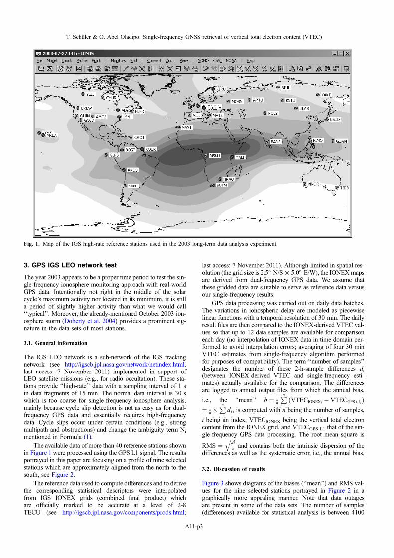
The available data of more than 40 reference stations shownin Figure 1 were processed using the GPS L1 signal. The resultsportrayed in this paper are focusing on a profile of nine selectedstations which are approximately aligned from the north to thesouth, see Figure 2.

The reference data used to compute differences and to derivethe corresponding statistical descriptors were interpolatedfrom IGS IONEX grids (combined final product) whichare officially marked to be accurate at a level of 2-8TECU (see http://igscb.jpl.nasa.gov/components/prods.html;

last access: 7 November 2011). Although limited in spatial res-olution (the grid size is 2.5� N/S · 5.0� E/W), the IONEXmapsare derived from dual-frequency GPS data. We assume thatthese gridded data are suitable to serve as reference data versusour single-frequency results.

GPS data processing was carried out on daily data batches.The variations in ionospheric delay are modeled as piecewiselinear functions with a temporal resolution of 30 min. The dailyresult files are then compared to the IONEX-derived VTEC val-ues so that up to 12 data samples are available for comparisoneach day (no interpolation of IONEX data in time domain per-formed to avoid interpolation errors; averaging of four 30 minVTEC estimates from single-frequency algorithm performedfor purposes of compatibility). The term ‘‘number of samples’’designates the number of these 2-h-sample differences di(between IONEX-derived VTEC and single-frequency esti-mates) actually available for the comparison. The differencesare logged to annual output files from which the annual bias,

i.e., the ‘‘mean’’ b ¼ 1n

Pni¼1

VTECIONEXi � VTECGPS L1ið Þ¼ 1

n�Pni¼1

di, is computed with n being the number of samples,

i being an index, VTECIONEX being the vertical total electroncontent from the IONEX grid, and VTECGPS L1 that of the sin-gle-frequency GPS data processing. The root mean square is

RMS ¼ffiffiffiffid2

in

qand contains both the intrinsic dispersion of the

differences as well as the systematic error, i.e., the annual bias.

3.2. Discussion of results

Figure 3 shows diagrams of the biases (‘‘mean’’) and RMS val-ues for the nine selected stations portrayed in Figure 2 in agraphically more appealing manner. Note that data outagesare present in some of the data sets. The number of samples(differences) available for statistical analysis is between 4100

Fig. 1. Map of the IGS high-rate reference stations used in the 2003 long-term data analysis experiment.

T. Schuler & O. Abel Oladipo: Single-frequency GNSS retrieval of vertical total electron content (VTEC)

A11-p3

and 4380 for four out of the nine presented sites. Slightly largerdata losses are linked to KIRU, VILL, and MAS1 (between3090 and 3180 samples), and the largest data outages occurredat MSKU (1453 samples) which was not recording data for thecomplete year 2003.

Typically, the RMS is between 1.4 and 2.3 TECU for thehigh- and mid-latitude sites which is a very promising resultin our eyes. Not unexpectedly, the RMS climbs up to valuesof 7.2 and 10.7 TECU for MAS1 and MSKU, respectively.Horizontal interpolation errors and mapping function inconsis-tencies yield higher deviations from the reference data. The glo-bal RMS is close to 4 TECU taking all IGS LEO tracking sites

into account. This is still in the 2–8 TECU boundaries of theuncertainty we have to expect for the reference data. However,please note that our statistical analysis can only depict the typ-ical annual mean performance of the single-frequency VTECretrieval algorithm. The accuracy of a single VTEC determina-tion can still show variations, e.g., as a function of local time,which cannot be revealed by our analysis.

The long-term bias of MSKU is the largest out of all nineselected stations, but it is also located closest to the geomag-netic equator where the diurnal variations are strongest and gra-dients are most expressed. Moreover, this station had to largestnumber of data outages. Anyway, the bias is still much smallerin magnitude than the RMS of this station.

4. Galileo E5 test trials

As mentioned in Section 1.1, code range accuracy is of majorimportance to obtain useful VTEC results with this single-fre-quency algorithm. With this respect, the dominant error sourceis multipath. Table 1 summarizes maximum and typical multi-path errors for selected signals for one specific type of correlatorcalled ‘‘Narrow Correlator’’ (van Dierendock et al. 1992) asbuilt into certain commercially available receivers.

The reader can see in the table that a number of new signalswill be available. The GPS L5 signal, for instance, will also fea-ture an increased multipath performance. Two modulation

Fig. 2. Selection of IGS network sites used for all diagrams in this paper; RMS ‘‘speedometer’’ visualization in (TECU) on the left and right.

Fig. 3. Diagram of VTEC biases and RMS in (TECU) for the GPSL1 results.

J. Space Weather Space Clim. 3 (2013) A11

A11-p4

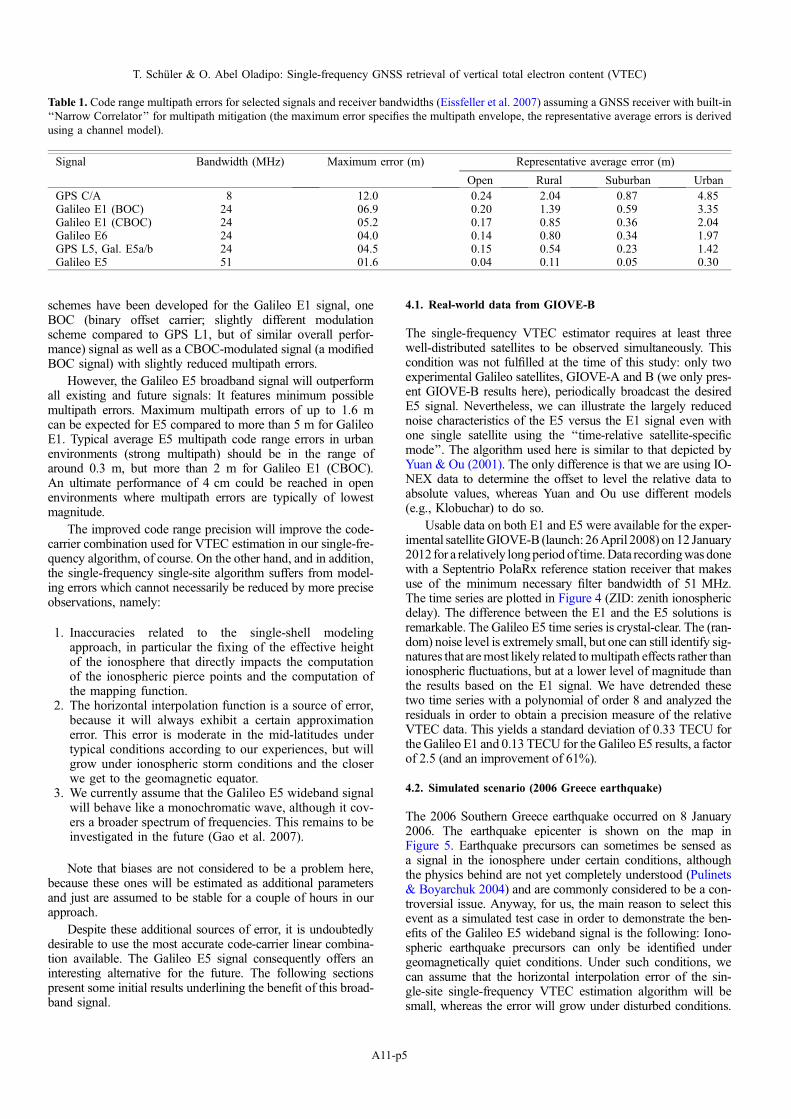
schemes have been developed for the Galileo E1 signal, oneBOC (binary offset carrier; slightly different modulationscheme compared to GPS L1, but of similar overall perfor-mance) signal as well as a CBOC-modulated signal (a modifiedBOC signal) with slightly reduced multipath errors.

However, the Galileo E5 broadband signal will outperformall existing and future signals: It features minimum possiblemultipath errors. Maximum multipath errors of up to 1.6 mcan be expected for E5 compared to more than 5 m for GalileoE1. Typical average E5 multipath code range errors in urbanenvironments (strong multipath) should be in the range ofaround 0.3 m, but more than 2 m for Galileo E1 (CBOC).An ultimate performance of 4 cm could be reached in openenvironments where multipath errors are typically of lowestmagnitude.

The improved code range precision will improve the code-carrier combination used for VTEC estimation in our single-fre-quency algorithm, of course. On the other hand, and in addition,the single-frequency single-site algorithm suffers from model-ing errors which cannot necessarily be reduced by more preciseobservations, namely:

1. Inaccuracies related to the single-shell modelingapproach, in particular the fixing of the effective heightof the ionosphere that directly impacts the computationof the ionospheric pierce points and the computation ofthe mapping function.

2. The horizontal interpolation function is a source of error,because it will always exhibit a certain approximationerror. This error is moderate in the mid-latitudes undertypical conditions according to our experiences, but willgrow under ionospheric storm conditions and the closerwe get to the geomagnetic equator.

3. We currently assume that the Galileo E5 wideband signalwill behave like a monochromatic wave, although it cov-ers a broader spectrum of frequencies. This remains to beinvestigated in the future (Gao et al. 2007).

Note that biases are not considered to be a problem here,because these ones will be estimated as additional parametersand just are assumed to be stable for a couple of hours in ourapproach.

Despite these additional sources of error, it is undoubtedlydesirable to use the most accurate code-carrier linear combina-tion available. The Galileo E5 signal consequently offers aninteresting alternative for the future. The following sectionspresent some initial results underlining the benefit of this broad-band signal.

4.1. Real-world data from GIOVE-B

The single-frequency VTEC estimator requires at least threewell-distributed satellites to be observed simultaneously. Thiscondition was not fulfilled at the time of this study: only twoexperimental Galileo satellites, GIOVE-A and B (we only pres-ent GIOVE-B results here), periodically broadcast the desiredE5 signal. Nevertheless, we can illustrate the largely reducednoise characteristics of the E5 versus the E1 signal even withone single satellite using the ‘‘time-relative satellite-specificmode’’. The algorithm used here is similar to that depicted byYuan & Ou (2001). The only difference is that we are using IO-NEX data to determine the offset to level the relative data toabsolute values, whereas Yuan and Ou use different models(e.g., Klobuchar) to do so.

Usable data on both E1 and E5 were available for the exper-imental satelliteGIOVE-B (launch: 26April 2008) on 12 January2012 for a relatively longperiod of time.Data recordingwas donewith a Septentrio PolaRx reference station receiver that makesuse of the minimum necessary filter bandwidth of 51 MHz.The time series are plotted in Figure 4 (ZID: zenith ionosphericdelay). The difference between the E1 and the E5 solutions isremarkable. The Galileo E5 time series is crystal-clear. The (ran-dom) noise level is extremely small, but one can still identify sig-natures that aremost likely related tomultipath effects rather thanionospheric fluctuations, but at a lower level of magnitude thanthe results based on the E1 signal. We have detrended thesetwo time series with a polynomial of order 8 and analyzed theresiduals in order to obtain a precision measure of the relativeVTEC data. This yields a standard deviation of 0.33 TECU forthe Galileo E1 and 0.13 TECU for the Galileo E5 results, a factorof 2.5 (and an improvement of 61%).

4.2. Simulated scenario (2006 Greece earthquake)

The 2006 Southern Greece earthquake occurred on 8 January2006. The earthquake epicenter is shown on the map inFigure 5. Earthquake precursors can sometimes be sensed asa signal in the ionosphere under certain conditions, althoughthe physics behind are not yet completely understood (Pulinets& Boyarchuk 2004) and are commonly considered to be a con-troversial issue. Anyway, for us, the main reason to select thisevent as a simulated test case in order to demonstrate the ben-efits of the Galileo E5 wideband signal is the following: Iono-spheric earthquake precursors can only be identified undergeomagnetically quiet conditions. Under such conditions, wecan assume that the horizontal interpolation error of the sin-gle-site single-frequency VTEC estimation algorithm will besmall, whereas the error will grow under disturbed conditions.

Table 1. Code range multipath errors for selected signals and receiver bandwidths (Eissfeller et al. 2007) assuming a GNSS receiver with built-in‘‘Narrow Correlator’’ for multipath mitigation (the maximum error specifies the multipath envelope, the representative average errors is derivedusing a channel model).

Signal Bandwidth (MHz) Maximum error (m) Representative average error (m)

Open Rural Suburban Urban

GPS C/A 8 12.0 0.24 2.04 0.87 4.85Galileo E1 (BOC) 24 06.9 0.20 1.39 0.59 3.35Galileo E1 (CBOC) 24 05.2 0.17 0.85 0.36 2.04Galileo E6 24 04.0 0.14 0.80 0.34 1.97GPS L5, Gal. E5a/b 24 04.5 0.15 0.54 0.23 1.42Galileo E5 51 01.6 0.04 0.11 0.05 0.30

T. Schuler & O. Abel Oladipo: Single-frequency GNSS retrieval of vertical total electron content (VTEC)

A11-p5

Hence we are able to separate data modeling errors from obser-vation uncertainties.

4.2.1. Data simulation

Simulated code range and carrier phase data for 7 days includ-ing several days before the seismic event were generated andanalyzed. These synthetic observations were generated with atemporal resolution of 5 s. The further simulation settings areas follows:

The random carrier phase noise is set to a minimum of0.6 mm and a maximum of 2 mm as a function of elevation.This corresponds to typical values for high-quality geodeticreceivers. The code range noise is assumed to be 11 cm forGalileo E1 (identical choice for GPS L1) and 1 cm for GalileoE5 in zenith direction following Avila-Rodriguez et al. (2004,Table 6). These minimum noise figures are mapped into slant

direction using an elevation-dependent exponential functionso that measurements close to the horizon are considerablynoisier than close to the zenith – an evident characteristic.

The multipath settings are taken from Eissfeller et al. (2007)and correspond to the values listed in Table 1: the maximumcode range multipath is set to 6.93 m for Galileo E1 and1.62 m for Galileo E5. The maximum carrier phase multipatherrors are set to 23.8 mm for Galileo E1 and 31.4 mm forGalileo E5. The fact that Galileo E5 exhibits a higher maximumerror on the carrier phase is linked to the phase shift induced bythe multipath. Since the wavelength of E5 is higher (25.2 cm)compared to E1 (19.0 cm), the resulting error in metric unitswill be higher, too. However, all these error values for the car-rier phases are of minor concern, because code range errors areclearly dominating. Similarly to the randomly distributed noisefigure, an elevation-dependent increase of the multipath error isto be expected. In our simulation we assume that 32% of themaximum error are typically present at an elevation angle of10�, and we set this ratio to 1.2% for values at zenith (whichis rarely reached by the Galileo satellites). These percentagesare taken from our experiences and approximately correspondto an environment at our University campus. Actually, wearrive at errors between 52 cm (at 10�) and (theoretically) 2cm (at 90�) for the E5 signal which approximately fits the typ-ical values stated in Table 1 for category ‘‘urban’’. Note that thetypical average elevation of a Galileo satellite is around 30� to35�. With this respect, our simulation settings are relatively pes-simistic, because there are also reference stations located in‘‘open’’ environments. At these locations, the results obtainedwith Galileo E5 single-frequency data analysis could be signif-icantly better than in our simulated scenario.

IGS IONEX maps were used to extract the ionosphericdelay information and feed the simulator. Biases are presentfor each satellite and are always part of the estimation modelof the single-frequency VTEC retrieval algorithm. As outlined

Fig. 5. The 2006 Greece earthquake epicenter (large cross) and thefour IGS/EUREF reference stations used in this test case.

Fig. 4. VTEC/ZID time series, Galileo/GIOVE-B E1 (left) and E5 (right), 12 January 2012

J. Space Weather Space Clim. 3 (2013) A11

A11-p6

before, no separation between receiver common biases andsatellite-specific ones is carried out, i.e., individual biases areestimated for each uninterrupted satellite arc.

4.2.2. Results

Since we want to outline the benefit of the improved measure-ment precision of the Galileo E5 data, we restrict the results to alook at the standard deviation of unit weight a priori (r0) and aposteriori (s0). The first is arbitrarily chosen as 1 m. The empir-ical a posteriori value is computed as s20 ¼ vT � P� v, where vis the vector of residuals and P is the weight matrix. The resultsobtained with the Galileo E5 data are listed in Table 2.

It is to be stressed that the standard deviation of unit weighta posteriori is not only defined by the measurement precisiononly, but can also be influenced by data mismodeling effects,of course. However, we have intentionally chosen a geomagnet-ically quiet period of time in order to make sure that such mod-eling artifacts are reduced to sufficient extent, so that the resultswe see should be in major parts related to the measurementprecision.

In average, the empirical standard deviation of unit weightis close to 10 cm for Galileo E5 and 38 cm for GPS L1 (nottabulated, because these values show little variability for theindividual stations). This underlines the increased precisionexpected for the Galileo E5 broadband signal. Moreover, wecan see that the minimum and maximum values in the caseof GPS L1 only show very marginal variations, whereas thevariations for the Galileo E5 results are higher (0.07 to0.15 m). The explanation for this fact is actually related tothe influence of modeling errors: These modeling uncertaintiesmap into both standard deviations, but in the case of the GPSL1 results, these errors are more or less completely hidden bythe relatively high observation noise, so the values do not showany strong numerical difference. This is a bit different from theGalileo E5 results. Here, the code range uncertainties are sosmall that modeling errors become visible in the numericalresults. Consequently, the standard deviation of unit weight aposteriori can differ from day to day (and from site to site)depending on the individual ionospheric conditions introducingdifferent modeling errors to the retrieval algorithm.

Clearly speaking, the mismodeling errors due to the limita-tions inherent in the horizontal interpolation algorithm and themapping function (single-layer model of the ionosphere) willincrease under unfortunate conditions such as ionospherestorms. In these cases, s0 will be in major parts influenced bythese modeling errors so that the advantage of the improvedcode range precision of the E5 observations is likely not toyield a significant gain in the overall accuracy of the results.This is a limitation of the single-frequency single-site algorithmrather than of the Galileo E5 signal. The benefits of E5 wide-band observations could still play an important role in net-work-based approaches in the future under such conditions.

5. Summary, conclusions, and outlook

The future global satellite navigation system Galileo will offeran outstanding signal in space, the E5 broadband signal, thatwill offer a code range accuracy, which is at least a factor oftwo up to a factor of 4 better than what we currently can expectfrom GPS L1 code range measurements. Unfortunately, thiswill be the only signal of that kind transmitted by the Galileosatellites. For this reason, we experimented with single-fre-quency single-site ionospheric delay estimation.

Despite the advances in measurement precision we expectfrom Galileo, we were surprised in a positive way by the VTECresults we could obtain from GPS real-world data for the year2003. Comparing the estimated results with those of IONEXdata from the IGS, a RMS of 4 TECU was obtained in globalaverage. Most mid- and high-latitude stations even exhibitsmaller RMS values of 1.5–2.5 TECU, whereas stations locatedwithin the geomagnetic equatorial belt normally show higherdeviations.

Real data of the GIOVE-B experimental Galileo satellitewere analyzed afterwards, demonstrating that a significantincrease in measurement precision can be expected in the nearfuture provided that the E5 AltBOC signal will be implementedin a similar manner as for GIOVE-B: the satellite-specificresults for E5 are a factor of 2.5 less noisy than the resultsobtained from E1 data (what approximately corresponds toGPS L1 data). Unfortunately, there are not enough Galileo sat-ellites in the sky yet (first half of year 2012) so that no absoluteVTEC retrieval is possible with E5 data. Results for a geomag-netically quiet period of time from simulated observations con-firm that the standard deviation of unit weight is significantlyreduced for the Galileo E5 results compared to that of E1.We expect this advantage to diminish under disturbed condi-tions or when moving toward the geomagnetic equator. Thereason for this fact is linked to the main data modeling errorsinherent in the single-frequency single-site approach: inaccura-cies related to the single-shell modeling approach directlyimpact the computation of the ionospheric pierce points andthe computation of the mapping function. Moreover, the hori-zontal interpolation function is a source of error, because it willalways exhibit a certain approximation error that will growunder disturbed conditions. Regarding the Galileo program,note that a full constellation of Galileo satellites is expectedto be in place around 2020, but four IOV satellites shouldalready be in orbit around the end of 2012 with an initial orbitconfiguration of 18 satellites to be ready around 2014–2016(interested readers can find updates at the European SpaceAgency’s web site http://www.esa.int/esaNA/galileo.html –see ‘‘Galileo Fact Sheet (PDF)’’ (last access: 27 September2012)).

Our future work regarding this single-site approach is tolink the retrieval algorithm with the NeQuick2 ray-tracer. Wehope to derive improved mapping function values via that

Table 2. Standard deviation of unit weight a posteriori (s0) for VTEC retrieval from synthetic Galileo E5 data; unit is meters.

Quantity Average Mate NOA1 NOT1 ORID

Mean 0.10 0.10 0.10 0.12 0.09RMS 0.11 0.10 0.10 0.12 0.10Minimum 0.07 0.07 0.07 0.08 0.07Maximum 0.13 0.14 0.11 0.15 0.13

T. Schuler & O. Abel Oladipo: Single-frequency GNSS retrieval of vertical total electron content (VTEC)

A11-p7

method, and to better account for variations in the vertical struc-ture of the ionosphere that is currently only modeled with onesite-specific effective height of the ionosphere, fixed for thecomplete year.

Acknowledgements. The authors would like to thank the IGS com-munity (International GNSS Service) for granting access to thehigh-rate dual-frequency GPS data of the IGS LEO network usedin this study. The financial support of the European Union and theEuropean GNSS Agency (GSA) in the framework of FP7 researchgrant ‘‘SX5 – Scientific Service Support based on Galileo E5Receivers’’ is highly appreciated. Trademarks possibly mentionedin the text are the property of their respective owners.

References

Avila-Rodriguez, J.-A., G.W.Hein,M. Irsigler, andT. Pany,CombinedGalileo/GPS Frequency, Signal Performance Analysis, Proceed-ings of the International Technical Meeting of the Satellite Divisionof the Institute of Navigation, ION GNSS, September 21–24, LongBeach, California, pp. 632–649, 2004.

Coco, D. S., C. Coker, S. R. Dahlke, and J. R. Clynch, Variability ofGPS satellite differential group delay biases, IEEE Trans. Aerosp.Electron. Syst., 27 (6), 931–938, 1991.

Cohen, C.E., B. Pervan, and B.W. Parkinson, Estimation of absoluteionospheric delay exclusively through single-frequency GPSmeasurements, Proceedings of the 5th International TechnicalMeeting of the Satellite Division of The Institute of Navigation(ION GPS 1992), September 16–18, Albuquerque, NM, USA, pp.325–329, 1992.

Dach, R., U. Hugentobler, P. Fridez, and M. Meindl, Bernese GPSSoftware Version 5.0 (User manual of the Bernese GPS SoftwareVersion 5.0), AIUB – Astronomical Institute, University of Bern,January 2007.

van Dierendonck, A.J., P. Fenton, and T. Ford, Theory andperformance of narrow correlator spacing in a GPS receiver,Navig. J. Inst. Navig., 39 (3), pp. 115–124, 1992.

Doherty, P., A.J. Coster, and W. Murtag, Space weather effects ofOctober to November 2003, GPS Solutions, 8 (4), 267–271, 2004.

Eissfeller, B., M. Irsigler, J. Avila-Rodriguez, E. Schuler, and T.Schuler, Das europaische Satellitennavigationssystem GALILEO– Entwicklungsstand, AVN – Allgemeine Vermessungsnachrich-ten, No. 02/2007, Wißner-Verlag, Germany, pp. 42–55, 2007.

Gao, G.X., S. Datta-Barua, T. Walter, and P. Enge, Ionosphere effectsfor wideband GNSS signals, Proceedings of the 63rd Annual

Meeting of The Institute of Navigation, Cambridge, pp. 147–155,2007.

Hoffmann-Wellenhof, B., H. Lichtenegger, and J. Collins, GPS –Theory and practice, 2nd ed., Springer, Wien, New York, ISBN3-211-82364-6, 1993.

Issler, J.-L., L. Ries, J.-M. Bourgeade, L. Lestarquit, and C.Macabiau, Probabilistic approach of frequency diversity asinterference mitigation means, Proceedings of ION GNSS 2004,17th International Technical Meeting of the Satellite Division, 21–24 September, Long Beach, CA, USA, pp. 2136–2145, 2004.

Leick, A., GPS Satellite Surveying, 2nd ed., John Wiley & Sons, Inc,New York, ISBN 0-471-30626-6, 1995.

Leick, A., GPS Satellite Surveying, 3rd ed., John Wiley & Sons, Inc,p. 464, ISBN 0-471-05930-7, 2004.

Lestarquit, L., N. Suard, and J.-L. Issler, Determination of theionospheric error using only L1 frequency GPS receiver,Proceedings of ION GPS-96, 9th International Technical Meetingof the Satellite Division of the Institute of Navigation, KansasCity Convention Center, September 17–20, Kansas City, USA,1996.

Mayer, C., N. Jakowski, J. Beckheinrich, and E. Engler, Mitigationof ionospheric range error in single-frequency GNSS applica-tions, Proceedings of ION GNSS 2008, 21st InternationalTechnical Meeting of the Satellite Division, 16–19 September,Savannah, Georgia, USA, pp. 2370–2375, 2008.

Nava, B., P. Coisson, and S. Radicella, A new version of theNeQuick ionosphere electron density model, J Atmos. Sol. Terr.Phys., 70 (15), 1856–1862, DOI: 10.1016/j.jastp.2008.01.015,2008.

Petit, G., B. Luzum, and IERS Conventions, IERS Technical NoteNo. 36. International Earth Rotation and Reference SystemsService (IERS), Verlag des Bundesamts fur Kartographie undGeodasie, Frankfurt am Main, 2010.

Pulinets, S., and B. Boyarchuk, Ionospheric precursors of earth-quakes, 1st ed., Springer, Berlin, ISBN 3-540-20839-9, 2004.

Xia, R., Determination of absolute ionospheric error using a singlefrequency GPS receiver, Proceedings of the 5th InternationalTechnical Meeting of the Satellite Division of The Institute ofNavigation (ION GPS 1992), September 16–18, Albuquerque,NM, USA, pp 483–490, 1992.

Yuan, Y., and J. Ou, An improvement to ionospheric delay correctionfor single-frequency GPS users – the APR-I scheme, J. Geod., 75,331–336, 2001.

Cite this article as: Schuler T & Abel Oladipo O: Single-frequency GNSS retrieval of vertical total electron content (VTEC) with GPSL1 and Galileo E5 measurements. J. Space Weather Space Clim., 2013, 3, A11.

J. Space Weather Space Clim. 3 (2013) A11

A11-p8