pca and fourier analysis - cornell...

Quantitative Understanding in Biology PCA and Fourier Analysis

Introduction Throughout this course we have seen examples of complex mathematical phenomena being represented as linear combinations of simpler phenomena. For example, the solution to a set of ordinary differential equations is expressed as a linear combination of exponential terms, with the weights given to each term determined by the eigenvectors and the initial conditions of the problem.

Linear combinations are especially useful because they allow us to apply the principle of superposition. This means we can decompose a complex system into a number of simpler systems. If we can understand the simpler systems, we can understand the complex system as a sum of the simpler ones. This idea is pervasive throughout mathematics, and we will be using this idea again today. But before we venture into new territory, we’ll formalize some probably already familiar notions about this idea of linear combinations.

Projections of Vectors When we are working in 2D Cartesian space, we represent points as a pair of numbers, such as (2, 3). This is so natural that we often don’t give it much thought, but in fact we are representing our vector as a linear combination of simpler entities. When we write (2, 3), at some level this is just a pair of numbers. Implicit in this representation, though, is the idea that the vector of interest is 2 parts and three parts , where and are unit vectors in the x and y directions, respectively. So when we see (2, 3), we think of . Hopefully, this does not come as a shock to anyone.

One way of thinking about arbitrary vectors and their relationship to and is in terms of projections. A projection is the mathematical equivalent of casting a shadow. If we think about the vector (2, 3), its projection on the x-axis (i.e., the shadow it would cast on the x-axis) is of length two. Similarly, its shadow cast on the y-axis is of length three. Note that to ‘cast a shadow’, we ‘shine light’ perpendicular to the axis upon which we want the shadow to cast. This is represented graphically in panel A of the figure below.

PCA and Fourier Analysis

Copyright 2008, 2010 – J Banfelder, Weill Cornell Medical College

Although the choice of and is quite natural, it is somewhat arbitrary. We might have chosen and , as shown in panel B. In this case, the projection of our vector on is negative and relatively small in

magnitude, whereas the projection of our vector on is relatively large. We see that we can represent a vector of interest in terms of linear combinations of and . You might want to do this if you were, say, solving a problem regarding an object sitting on a 45˚ incline, so the coefficient of represents its position on the surface and the coefficient of represents its ‘altitude’ (memories of physics problems should be resurfacing now). Of course, if you want to do this formally, we will need to be a bit more quantitative.

The mathematical way to compute a projection is to take the inner product, also known as the dot product, of the vector of interest with the so-called basis vector. In the example in the figure, we have…



Basis Sets in Cartesian Space The set of vectors we use in linear combinations to express an arbitrary vector is called a basis set. A good basis set has three important properties:

• members of the basis set are orthogonal

• members of the basis are normalized

• some linear combination of the members of the basis set can represent any arbitrary object in the space of interest

Let’s review each of these properties in turn. We’ll begin with the property of orthogonality. This means that the projection of each element of the basis set on all of the others should be zero. For the classic Cartesian basis set, we have…

…and for our rotated coordinate system we have…

We see that both basis sets are orthogonal. Note that the eigenvectors of an arbitrary matrix are not necessarily orthogonal. This does not mean you can’t use them as a basis set, it is just that they lack a certain convenience.

Next we consider the property of normality. In a normalized basis set, the projection of each element of the basis set on itself will be unity. Again, we consider the classic Cartesian basis set…

…and our rotated system…

Again, both basis sets are normalized. Normalizing a basis set is usually pretty easy, as all you have to do is multiply each element of the set by a constant so the inner products work out to unity. For example, if



we had chosen = (1, 1) and , we would have found that = 2; and we would have

corrected this by multiplying by (and similarly for ).

The last property is completeness. It is easy to see that as long as the two basis vectors we are considering are linearly independent they will be sufficient to represent any 2D vector. However, if we were interested in 3D space, then two vectors wouldn’t cut it. The projection of a 3D vector onto two 2D vectors gives us the best possible representation given the incomplete basis set, but it is not quite good enough for a full representation of the data in the original 3D vector. We lose information in such a projection.

Your hand casting a shadow on a wall is an example of an incomplete projection. Every point that makes up your hand is mapped to a 2D space (the surface upon which your shadow is cast). Given a shadow, you cannot reproduce a whole hand. You can choose different incomplete basis sets by moving the light source (or alternatively rotating your hand); you will get different projections, but none will be complete.

Basis sets that satisfy all three conditions are called complete orthonormal basis sets. We should note that the terminology we are using here is that commonly used by chemists. A mathematician would say that a basis is, by definition, complete. While the terminology may change from domain to domain, the ideas don’t.

A Diversion into Principal Components Analysis Sometimes using an incomplete basis set can be advantageous. When dealing with large datasets, we often seek to reduce the amount of data we deal with. Say you’ve collected three variables per observation in an experiment, and you’re looking to reduce the amount of data you deal with. You could choose to ignore one of these variables (say the third: the z-value). This is equivalent to projecting your 3D (x,y,z) dataset onto the 2D (x,y) plane. Of course, you could eliminate any of the other variables, by projecting onto the (x,z) or (y,z) planes.

Once you start thinking of reducing your data as projecting high-dimensional vectors onto a lower dimensional plane, it becomes natural to think about projecting onto planes that don’t correspond to the coordinate axes. Maybe, instead of dropping one or another variable altogether, we can find a 2D plane upon which we project our 3D data that results in a minimal loss of information. This is the essence of principle components analysis, or PCA.

To understand how PCA works, we need to recall the concepts of variance and correlation. Recall that the variance of a sample is given by

We can define the covariance between two variables, x and y, as…



This is a lot like the Pearson correlation coefficient (Pearson invented PCA). Recall that when x varies with y, this expression will tend to accumulate positive terms. When x and y are independent, the covariance will tend to zero, and when x and y are anti-correlated, a negative quantity will result. Note that the variance of a variable is just the covariance of that variable with itself.

In higher-dimensional spaces, we can compute the covariance of every variable with every other variable. These values can be arranged in a square matrix, the size of which will be the number of dimensions of the original data. The diagonal terms will be the variances of the individual variables. The off diagonal terms will be near zero if the underlying variables are uncorrelated, and will be large if there is significant correlation.

We can demonstrate this idea in Matlab. We begin be creating a dataset, a, with two independent (uncorrelated) values of 500 observations…

>> n=500; >> a(:,1) = normrnd(0,1,n,1); >> a(:,2) = normrnd(0,1,n,1); >> plot(a(:,1),a(:,2),'.') >> cov(a) ans = 1.0255 -0.0057 -0.0057 1.0072 Now, we synthesize a new dataset that has significant correlation. Note the values in the second column are an average of the value in the first column with a random component.

>> b(:,1) = normrnd(0,1,n,1); >> b(:,2) = 0.5*b(:,1) + 0.5*normrnd(0,1,n,1); >> plot(b(:,1),b(:,2),'.') >> cov(b) ans = 0.9598 0.5038 0.5038 0.5300 We see that the covariance matrix has strong off-diagonal terms.

Now for the magic of PCA. We want to know which line we can project our data onto to preserve the maximum variation in our data. It turns out that the eigenvectors and the eigenvalues of the covariance matrix give us the answer!

>> [V,D] = eig(cov(b))



V = 0.5512 -0.8344 -0.8344 -0.5512 D = 0.1972 0 0 1.2927 This tells us that the first principal component (the one with the largest eigenvector) is in the direction (0.83, 0.55). We can add that vector to our plot:

>> plot(b(:,1),b(:,2),'.') >> hold on >> V1 = V(:,2) V1 = -0.8344 -0.5512 >> plot([-V1(1), V1(1)],[-V1(2), V1(2)],'k') Projecting onto this line will give us the projection with the largest amount of variation. It also turns out that you can quantify the amount of variation that you preserve. The fraction of variation in the original data that is embedded in any particular principal component is simply the ratio of the eigenvalue of that component divided by the sum of all of the eigenvalues. So here we would be preserving 1.2927/(1.2927+0.1972) = 87% of the variation in the data while retaining only 50% of the data.

Matlab will do all of this work, and the translation to PC coordinates, in one command (including ordering the eigenvalues)…

>> [pcs, trans, evs] = princomp(b);

The first result contains the principal components, the second contains the transformed values, and the third contains the eigenvalues (in order).

In addition to data reduction, analysis in principal components can sometimes by informative. Suppose, for example, you were studying heart disease and its relationship to obesity, and had collected the height and weight of a number of patients. Since weight tends to correlate with height, you might perform a PCA, and test to see if any of the principal components correlate with heart disease. (Typically one uses BMI which is proportional to (weight/height2).



Representing Mathematical Functions as Linear Combinations of Basis Functions All this talk of basis sets in the context of points in 2D and 3D space should be relatively straightforward to grasp. Formalizing the ideas was a warm-up to using them in a somewhat less intuitive context: that of representing mathematical functions. Now, instead of representing points in space, we are trying to represent functions (or curves). Our task is to represent an arbitrary function as a linear combination of other, simpler functions. If we choose the simpler functions judiciously, we may gain insight.

In fact, we have already seen this idea at work once. When we looked at the linearization of a function using a Taylor series, we represented an arbitrary function as an infinite series of polynomial terms. The set of polynomials was our (infinitely long) basis set. When we truncated the Taylor series after the second term, we switched to an incomplete basis set. Note that the set of polynomials is not orthonormal, but the infinite set is nevertheless complete.

One example of the use of basis functions that is applicable to biology is found in quantum chemistry. The basic problem is to solve the Schrödinger equation (a partial differential equation in three dimensions) to get the density of electrons in a molecule (actually you want the ‘wavefunction’, the square of which gives the electron density). This can be done analytically only for really simple cases (such as a hydrogen atom). There are different solutions for different energy levels, which result in the s, p, d, f, g etc. orbitals, which are shown in the left panel below.

In modern quantum chemistry we want to solve the Schrödinger equation for biomolecules, for which there is no analytical solution known. The technique used is to approximate the molecular wavefunction as a linear combination of these hydrogen atomic orbitals. You pick some subset of the equations for hydrogen orbitals (you often don’t need the high-energy f and g orbitals for low energy problems with low atomic number nuclei), apply coordinate transformations so they are centered on each nucleus in your biomolecule, and then find the linear combination of those orbitals that best satisfies the



Schrödinger equation. For benzene, you get something like what is shown on the right panel of the above figure.

While the implementation and mathematics behind this is quite complex, the ideas here should be familiar to you. By expressing the solution to a complex problem as a linear combination of solutions to simpler ones, we often get decent, if not completely correct, answer (think back to our work on sets of difference equations and eigensystems). Additionally, we are able to think of the solution as decomposed into parts. The whole idea of a molecular orbital as a combination of atomic orbitals is just a mathematical construct that helps us think about the solution in terms of parts we can grasp.

Fourier Representations of Mathematical Functions One common way to decompose a complex mathematical function is to represent it as a linear combination of sines and cosines at ever increasing frequencies. Such an infinite series of sines and cosines is called a Fourier series. One caveat of Fourier analysis is that we are only interested in what the function does over a particular interval; usually we imagine that the function will repeat itself from interval to interval (as sines and cosines tend to do). If we can decompose a function into its constituent sines and cosines, we can talk about the frequency content of that function. Usually the function in question is a time dependent signal; the analysis and manipulation of the frequency content of such signals is known as the art of signal processing. Quite a few image processing techniques use 2D or 3D extensions of these ideas. In fact, MRI machines acquire their raw data in the frequency domain, and the images we see are reconstructed by combining sines and cosines. For now, we will only consider 1D cases.

One of the very convenient things about Fourier represention is that an infinite series of sines and cosines represents a complete orthonormal basis set for a function over a specified interval. This means that we can exactly represent any function over an interval of interest as a mixture of sines and cosines in various proportions. In particular, for the interval [-π, π], almost any function can be represented by a series of the form…

We just have to find the ans and bns that give us the function we want. You can think about this series as a linear combination of basis functions: cos(nx) and sin(nx). The constant term can be folded into the basis set if you change the lower limits of the summations to zero. When n=0, cos(nx) is always unity so you’ll get a0 times one. Conversely, sin(nx) will always be zero, and the value of b0 will be irrelevant.

To represent a function of interest, we need to take the projection of our function, f(x), onto each of these basis functions. To do this, we take the integral of the product of our function with the basis function of interest over the interval we are studying: [-π, π]. If you don’t like this interval, you can always apply a variable transformation. Formally, we write…



Normally you will see a third equation in the literature for the a0 case, but this isn’t strictly necessary as it is already covered by the first equation above.

You may also run across formulations where the interval is [0, 2π], but the ideas are the same.

Here we have introduced the idea of the inner product being the integral of the product of the function of interest and the basis function without much comment. It is interesting to note that this formulation is the continuous analog of the inner product for vectors. When dealing with vectors, the inner product is defined as the sum of the pairwise products of the vector elements. If you recall that an integral is a continuous summation, then the idea of a projection of one function on another as the integral of their product is the natural extension of the case. Alternatively, you can think of a function over an interval as a vector of infinite length. The function f(x) over the interval can be represented (albeit not very practically) as the vector…

…but with infinitely more precision.

Discrete Signals and the Fast Fourier Transform All of the above is nice in theory, but has less practical application than you might think. While there is nothing wrong with the theory that we have developed, in reality we do not deal with continuous functions like f(x), but rather with discretely sampled signals. The sampling process has a profound effect on our results. The topic is complex, but can be distilled down to the observation that you need to sample a signal at a rate that is sufficient to capture the data you are looking for. You can’t sample a fast, high-frequency process with a low sample rate and expect to get meaningful results.

Processing discretely sampled signals is the job of the Fast Fourier Transform, or FFT. Matlab has this capability built in, and we will demonstrate its use here. Consider a signal that is a 1 Hz sine wave, sampled at a frequency of 10 Hz. We’ll generate data for one period in Matlab.

>> N = 10; %% number of sample points >> T = 1.0; %% time span of our samples



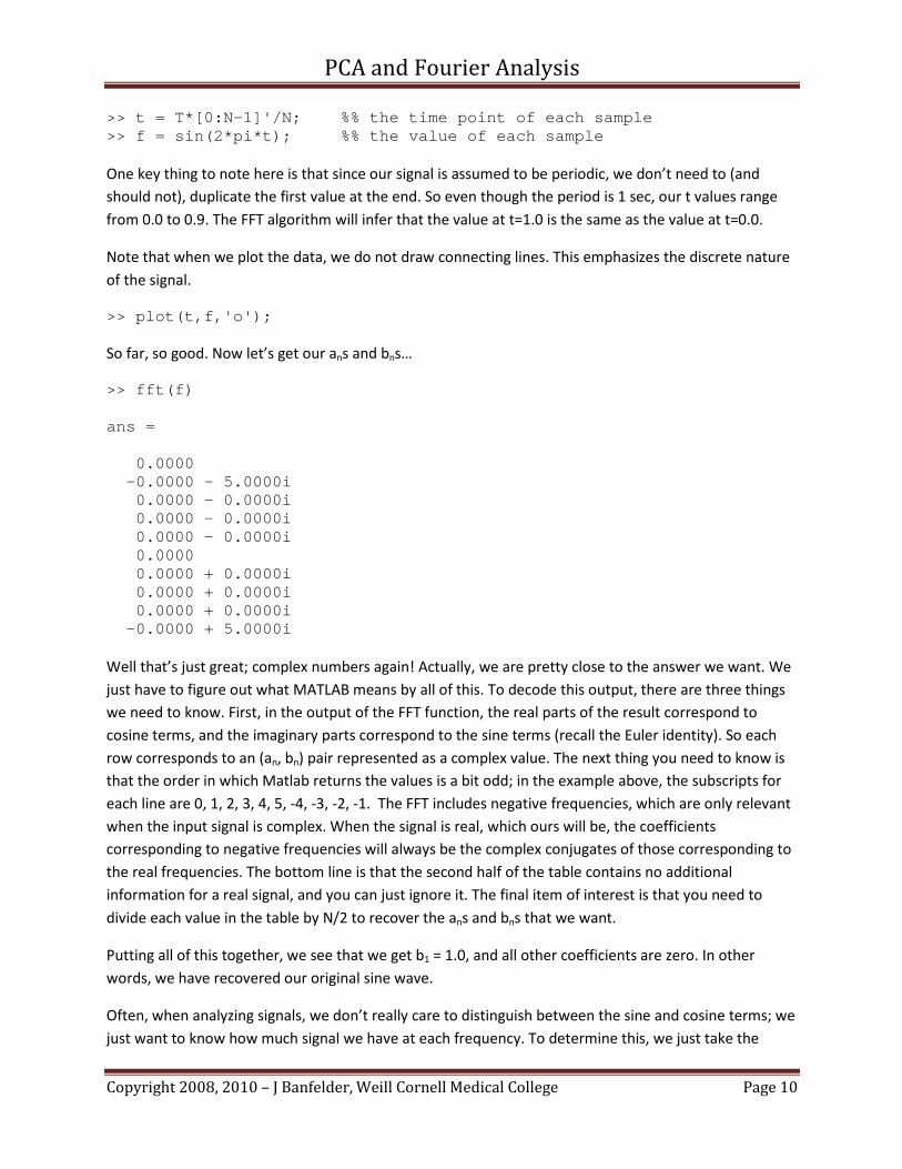
>> t = T*[0:N-1]'/N; %% the time point of each sample >> f = sin(2*pi*t); %% the value of each sample One key thing to note here is that since our signal is assumed to be periodic, we don’t need to (and should not), duplicate the first value at the end. So even though the period is 1 sec, our t values range from 0.0 to 0.9. The FFT algorithm will infer that the value at t=1.0 is the same as the value at t=0.0.

Note that when we plot the data, we do not draw connecting lines. This emphasizes the discrete nature of the signal.

>> plot(t,f,'o');

So far, so good. Now let’s get our ans and bns…

>> fft(f) ans = 0.0000 -0.0000 - 5.0000i 0.0000 - 0.0000i 0.0000 - 0.0000i 0.0000 - 0.0000i 0.0000 0.0000 + 0.0000i 0.0000 + 0.0000i 0.0000 + 0.0000i -0.0000 + 5.0000i Well that’s just great; complex numbers again! Actually, we are pretty close to the answer we want. We just have to figure out what MATLAB means by all of this. To decode this output, there are three things we need to know. First, in the output of the FFT function, the real parts of the result correspond to cosine terms, and the imaginary parts correspond to the sine terms (recall the Euler identity). So each row corresponds to an (an, bn) pair represented as a complex value. The next thing you need to know is that the order in which Matlab returns the values is a bit odd; in the example above, the subscripts for each line are 0, 1, 2, 3, 4, 5, -4, -3, -2, -1. The FFT includes negative frequencies, which are only relevant when the input signal is complex. When the signal is real, which ours will be, the coefficients corresponding to negative frequencies will always be the complex conjugates of those corresponding to the real frequencies. The bottom line is that the second half of the table contains no additional information for a real signal, and you can just ignore it. The final item of interest is that you need to divide each value in the table by N/2 to recover the ans and bns that we want.

Putting all of this together, we see that we get b1 = 1.0, and all other coefficients are zero. In other words, we have recovered our original sine wave.

Often, when analyzing signals, we don’t really care to distinguish between the sine and cosine terms; we just want to know how much signal we have at each frequency. To determine this, we just take the



norm of each coefficient. Frequency content is usually measured as the square of the norm, and this is what we are after. Matlab will compute our power spectrum as follows…

>> p = abs(fft(f))/(N/2); >> p = p(1:N/2).^2 p = 0.0000 1.0000 0.0000 0.0000 0.0000 The frequency corresponding to each value in the power spectrum can also be computed…

>> freq = [0:N/2-1]'/T freq = 0 1 2 3 4 Note that frequencies over 4 Hz are not reported. We’d have to sample more often to extract that information from our signal.

Let’s try a more complex case now. We’ll consider a combination of a 10 Hz signal and a 30 Hz signal. We’ll sample at 1 kHz for 3.4 seconds.

>> N = 3400; >> T = 3.4; >> t = T*[0:N-1]'/N; >> f = sin(2*pi*10*t) - 0.3*cos(2*pi*30*t); >> plot(t,f,'.'); >> p = abs(fft(f))/(N/2); >> p = p(1:N/2).^2; >> freq = [0:N/2-1]'/T; >> semilogy(freq,p,’.’); >> axis([0 50 0 1]); Here we can see strong frequency components at 10 Hz and 30 Hz; the rest is roundoff error (power values ~ 10-30 and below). Note the use of the semilog plot.

Let’s see what happens when we undersample. Consider an 11 Hz signal, sampled at 10 Hz for one second.

>> N = 10;



>> T = 1.0; >> t = T*[0:N-1]'/N; >> f = sin(2*pi*11*t); >> p = abs(fft(f))/(N/2); >> p = p(1:N/2).^2; >> freq = [0:N/2-1]'/T; >> semilogy(freq,p,'o'); The 11 Hz signal appears to have power at 1 Hz. This is an artifact of under sampling called aliasing. It is instructive to plot this function at high resolution and then just the points sampled here. Let’s plot the same underlying signal sampled at a much higher frequency…

>> N2 = 1000; >> t2 = T*[0:N2-1]'/N2; >> f2 = sin(2*pi*11*t2); >> plot(t2,f2); …and then overlay the results of our under-sampling…

>> hold on >> plot(t,f,'o'); Now you should appreciate why we shouldn’t draw lines connecting successive points in sampled data.

An important theoretical result related to our experiment here is the sampling theorem, which states that you can avoid aliasing effects as demonstrated here by ensuring that your sampling rate is at least twice that of the highest frequency component of the underlying signal.

Filtering and Compression Once you have your hands on the power spectrum (or the ans and bns of the Fourier expansion), you are in a position to do all kinds of filtering in the frequency domain.

For example, many experiments that involve electronic equipment will produce signal with a strong peak at 60 Hz because that is the frequency at which alternating current power is supplied. If you want to get rid of that artifact in your data, you can transform your signal into the frequency domain, zero out or reduce the value corresponding to 60 Hz, and reconstitute the signal.

You can also filter out high or low frequency noise (or unwanted signal) just by zeroing out parts of the power spectrum. All kinds of filters can be invented; filter design is a big part of signal processing.

Note that an FFT produces as many coefficients as there are samples in the original data. One means of compressing a signal is to compute its transform and simply drop, or forget about coefficients with small magnitudes. When you reconstitute the signal based on this reduced set of coefficients, you get pretty close to the original signal. In our two frequency samples above, we were able to reduce the whole sequence of 3,400 numbers down to two. Of course, if your original data is not synthesized from sines



and cosines, you will have more than just two terms. Many image compression algorithms are based on a 2D extension of this technique.

Fun With FFTs You can have some fun with FFTs in Matlab. Matlab can read some .wav sound files, and you can use its FFT functions to play with them. In the example below we read in a .wav file. Its length is adjusted to have an even number of samples.

>> f = wavread('sucker.wav'); >> length(f) ans = 330099 >> f(length(f)+1) = 0; >> N = length(f) N = 330100 To proceed with the analysis, you need to know the frequency at which the audio was sampled. In this case it is 22 kHz (the file properties in your OS will usually tell you this). You can play the file right from Matlab (who needs iTunes when you’ve got Matlab?)…

>> wavplay(f, 22000)

…and plot the waveform…

>> T = length(f)/22000 T = 15.0045 >> t = T*[0:N-1]'/N; >> plot(t,f); This is just a plot of the amplitude as a function of time, sampled at 22 kHz. You can easily see the short pauses between words.

Now let’s take an FFT of this signal and plot the power spectrum. We plot on both semilog axes and regular axes.

>> fs = fft(f); >> p = abs(fs)/(N/2); >> p = p(1:N/2).^2;



>> freq = [0:N/2-1]'/T; >> semilogy(freq,p); >> plot(freq,p); Here we see that most of the power is at less than 1 kHz, and that there is almost no power over 4 kHz. Let’s clip out all frequencies greater than about 2 kHz. This corresponds to roughly the 30,000th frequency in the FFT (15 sec * 2000 Hz) = 30, 000.

for i = 1:(N/2-30000) fs((N/2)+i)=0; fs((N/2)+1-i)=0; end p = abs(fs)/(N/2); p = p(1:N/2).^2; semilogy(freq,p); Now we can reconstitute the signal and play it. There are two things to note here. First, we only take the real parts of the inverse FFT. This should be purely real, but there are some rounding errors. Second, since we cut out a bit of the power in the signal, we’ll add a bit back in by multiplying the amplitude of the reconstituted signal.

>> filtered = real(ifft(fs)); >> wavplay(filtered*3,22000) Note that this sounds a bit muffled. But even with half of the data gone, it is still intelligible, if not at CD

quality. This is pretty amazing considering that we threw out 91% of the data in our orginal .wav file.

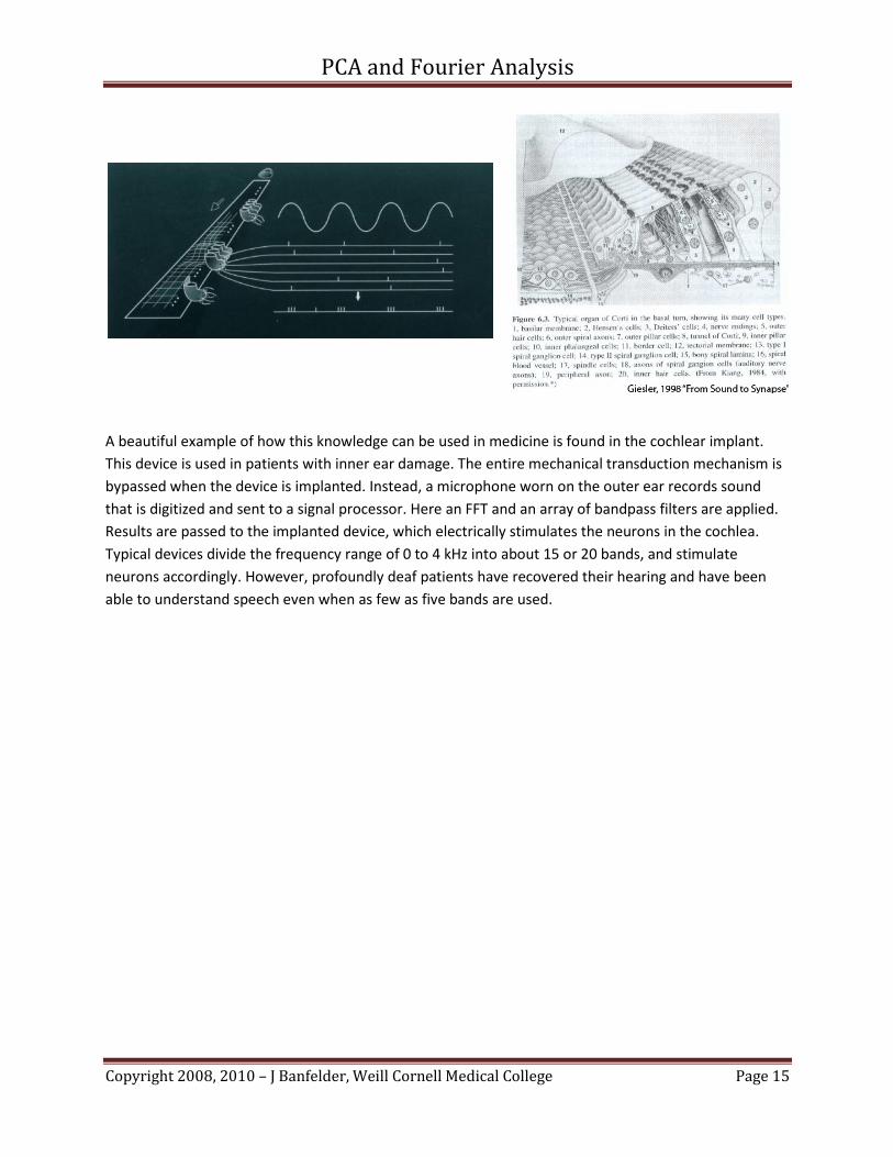
The Human Ear and Cochlear Implants All of this actually does have something to do with biology. Consider the human ear, which we just used! Here, part of the system is mechanical. In the ear, after sound is transduced into the cochlea, vibrations impinge on the basalar membrane. This membrane varies in width and stiffness along its length in such a manner that various parts of it will resonate at various frequencies. Cilia on the basilar membrane shear against a second membrane, the tectorial membrane. Bending of the cilia results in the release of a neurotransmitter which passes into the synapses of one or more nerve cells; this invokes an action potential in those neurons. The net result is that specific groups of neurons fire in response to the frequency content of the impinging sound. In essence, basalar membrane acts as a mechanical FFT algorithm, and the array of cilia and neurons act as a bank of bandpass filters. When you hear sounds such as music and speech, your brain is receiving a bank of action potentials that correspond to the FFTs we just learned about.



A beautiful example of how this knowledge can be used in medicine is found in the cochlear implant. This device is used in patients with inner ear damage. The entire mechanical transduction mechanism is bypassed when the device is implanted. Instead, a microphone worn on the outer ear records sound that is digitized and sent to a signal processor. Here an FFT and an array of bandpass filters are applied. Results are passed to the implanted device, which electrically stimulates the neurons in the cochlea. Typical devices divide the frequency range of 0 to 4 kHz into about 15 or 20 bands, and stimulate neurons accordingly. However, profoundly deaf patients have recovered their hearing and have been able to understand speech even when as few as five bands are used.

pca and fourier analysis - cornell...

Documents