pbio3250l: the dynamic genome spring 2010
TRANSCRIPT
PBIO3250L: The Dynamic Genome Spring 2010
Table of Contents
Syllabus Grading Policy Chapter 1: Background on Information Transfer and Experiment 1: Actin gene annotation 1-98 A. Background 1-14 B. PubMed 15-19 C. Experiment 1: Actin gene 20-34 D. Genomic and cDNA sequence analysis 35-47 E. Actin in Maize Genome 49-58 F. Gene Families 65-83 G. Rice Actin Homologs 85-98 Chapter 2: The Discovery of TEs and Experiment 2: mPing 99-140 A. Background 99-118 B. Characterizing TE Families 119-126 B. Experimental Design 127-135 C. Protocol for Experiment 2 136-140 Chapter 3: Epigenetics 139-151 A. Background 139-146 B. Experiment 146-151 Chapter 4: Exploring human genetic diversity: Alu 153-156 Chapter 5: Exploring MITE insertion sites 157-179 A. Step1: Genomic DNA Extraction 157-159 B. Step 2: Restriction/Ligation 161-162 C. Step 3: Primary Amplification 163 D. Step 4: Secondary Amplification 164-165 E. Step 5: PAGE 165 F. Step 6: Recovering PCR bands 167-172 G. Step 7: Analyzing results 173-179

Syllabus Spring 2010
Syllabus Grading Data
Lecture Lab Download
Thurs.,Jan 7
Course AdminCourseOverviewPubMed
Lab SafetyPipetting
Tues.,Jan 12
InformationFlowGenomics?
ExtractGenomicDNA
Chapter 13 IGA
Thurs.,Jan 14
GenomicsMaking ofFittest Ch. 1
Gel of DNANanodrop CURE Survey
Tues.,Jan 19
PCR Overview,cDNA (21-23)Making ofFittest Ch. 2and 3
PCR Rxnsetup (28-29)Pour Gels
Dolan DNALearningCenter PCRAnimation

Thurs.,Jan 21
SequencingOverview (pg30-34)Genomics(Chap. 13 IGA,453-468)
Gel PCR (2%gel)SequencingRxns (pg 30withchanges)
DNA SequencePpt
QUIZ I
Tues.,Jan 26
SequenceAnalysis
blastn (pg40)blast2seq(pg 44)MSA (pg59)
Thurs.,Jan 28
Gene Familiesand Trees
MaizeBrowse(pg 49)Maize
HomeworkI DueFriday at 5P.M.
Tues.,Feb 2
Gene Familiescont.
RicePrimerDesignRiceActingenes
Making ofFittest
Extract RiceGenomic DNA
RNAExtractionProtocol
QUIZ IRe-do

Thurs.,Feb 4
TEIntroductionMaking ofFittest Ch. 4-10
CheckGenomicDNAPCR Riceactin genes
Start readingThe GreatestShow on Earth
Tues.,Feb 9
TE FamiliesPing/mPingCharacterizerice TEs
Rice PCR gelsSequencing
WednesdaySue's GeneticsSeminar"Understandingthe other bigbang: howtransposableelementsamplifythroughoutgenomes" 4:00PM S175Coverdell. 10bonus pointsfor attendingand submittingsummary oftalk (500words max).
HomeworkII DueWednesdayat 6 P.M.
Thurs.,Feb 11
Ping/mPingexperiment
Greatest Discussion1 (1,2)
ObserveArabidopsisExtractArabidopsisDNA
QUIZ II
Tues.,Feb 16
Finish DNAPreps

Feb 16PCR
Thurs.,Feb 18
Analyze Ping results
Greatest Discussion2 (3)
Gels/AnalysisGerminateMuDr seeds
Report 1Guidelines
Tues.,Feb 23
Mid-Term Review Work on report Mid-TermReview Sheet
HomeworkIII DueMonday atnoon or 6p.m.
QUIZ III
Thurs.,Feb 25
Mid-Term Exam
Greenhouseand tourPlantarabidopsisRice
Mid-TermVersion AMid-TermVersion BMid-TermVersion C
Tues.,Mar 2
Epigenetics
SNOW DAY
Draft ofmini-report,Moday,Mar 1, by6:00 pm
SemesterMid-Term
EpigeneticsFinalversion

Thurs.,Mar 4
Epigenetics
Greatest Discussion3 (4,5)
Extract DNAPCR?
report dueby 6:00 pmon FridayMarch 5.
Tues.,Mar 9
SPRING BREAK!!! SPRINGBREAK!!!
Thurs.,Mar 11
SPRING BREAK!!! SPRINGBREAK!!!
Tues.,Mar 16
Greatest Discussion4 (6,7)
PCR/GelEpigeneticsAlu
Thurs.,Mar 18
Alu
Tues.,Mar 23
Greatest Discussion5 (8,9)
Alu-PCRSetup digeston 225
Thurs.,Mar 25
GreatestDiscussion 5(10-13)Alu-analyzedata
Alu-Gel
Tues.,Mar 30
Project overview
TD Step 1:Extract DNA
Homework due,Mon. 29 bynoon.

Thurs.,Apr 1 TD Step 2: R/L
Dawkins Essaydue Friday bynoon
Tues.,Apr 6
TD Step 3:Primary PCR
TD Step 4:Secondary PCR(hired help onWeds.)
Report 2Guidelines
Thurs.,Apr 8
TD Step 5: RunGel
Tues.Apr 13
Skype with SeanCarroll
TD Step 6: Getbands, amplify, gel
Bring 2questions fromMaking ofFittest to class(Quiz grade).
Thurs.,Apr 15
Topo clone
Tues.,Apr 20
Miniprep
Thurs.,Apr 22
Seq analysis.
FiguresQuiz IV
Tues.,Apr 27
Course review, workon papers CURE Survey
Tues,Final, gradedpaper to Ryan

Tues,May 4
FINAL 12:30. paper to RyanWeds by 5:00PM

Syllabus i
BIO/PBIO 3250L The Dynamic Genome Spring 2010
Dr Susan Wessler and Dr Jim Burnette Ryan McCarthy, TA
Course website: http://www.dynamicgenome.org/classes/spring_10/ User: dynamicgenome Password: tesjump
Office Phone Hours E-‐mail
Dr. Susan Wessler Plant Sciences 4510
706-‐542-‐1870 By appointment
Dr. Jim Burnette Plant Sciences 1506
706-‐542-‐4581 By appointment
Ryan McCarthy Plant Sciences 3507
706-‐542-‐5622 By appointment
[email protected] Attendance: We require 100% attendance and class participation. Any missed lab will be difficult to make up. If you know you will be absent for any class, make arrangements in advance with Dr. Burnette. Discuss unplanned absences immediately upon returning to class. If you have a fever DO NOT come to class. Call Dr. Burnette and go to the Health Center. DO NOT return to class until 24 hours AFTER all symptoms disappear. (CDC recommendation for limiting the spread of H1N1 flu.) Class participation is a major part of this course. You are expected to be prepared for each day, participate in all discussions, and ask a lot of questions. Twenty percent of your grade is based on class participation. Restrict cell phone/texting/earphone use and personal web browsing/e-‐mail to breaks. Cell phones should not be on your desk or lab bench at any other time. Do not use class time to work on assignments for other classes. Do not listen to music with earphones during lab work. We will provide a stereo for the whole lab. Use of cell phones at inappropriate times will result in a 5 point deduction per infraction from your participation grade. The syllabus and other handouts can be found on the website link above. This class has a very fluid schedule and the syllabus will change. Refer to the online syllabus for what will be covered in class. Page numbers, additional handouts, and experiments to be done will be posted on the Syllabus. In the computer lab, place your backpacks in the cubbyholes. For your safety, you must wear closed toe shoes (no flip-‐flops or sandals). Long shorts are permitted. Long hair should be pulled back away from the face for all labs. Eating is permitted in the computer lab (room 1503A) but not the wet lab (room 1606).

Syllabus ii
Assignments Notebook Checks
As needed. Quizzes Will be announced at least one class prior to quiz day. Homework Will be assigned with ample time for completion. Homework must be completed individually. Mid-‐Term (1.5 hour exam) Will include computer use. Thursday, February 25 in class. Final (1.5 hours) The final will be comprehensive and will include computer use. Tuesday, May 4 at 12:30. Reports There will be three written reports. Reports must be an individual effort. PBIO3250L is a writing intensive course. You will be guided through the writing process with the opportunity to revise at least twice before the report is graded. The drafts will not be graded but failure to turn in a draft will deduct from your final grade on the section. Failure to turn in one draft is a 5-‐point reduction and failure to turn in two drafts is a 10-‐point reduction from the final grade of the part. For more about the WIP program see this website: http://www.wip.uga.edu/ Final Project This may be in the form of a scientific poster or slide presentation. Grading Percentages: The final grade percentage will be calculated using this break down. Notebook check 10.0% Quiz average 10.0% Homework average 15.0% Report 15.0% Mid-‐Term 10.0% Final Project 10.0% Final 10.0% Participation 20.0% 100.0% Letter Grades: Letter grades will be assigned using the standard plus/minus system: A=95-‐100, A-‐=90-‐94, B+=86-‐89, B=83-‐85, B-‐=80-‐82, C+=76-‐79, C=73-‐75, C-‐=70-‐72, D=60-‐69, F<60. Remember the + or – is dropped for HOPE Scholarship GPA determination.

Chromatin
Metaphase chromosomes
eight histone proteins
Chromatin
Nucleosome
DNA double helix
What is the Genome? 1

Base Pairs
A
B
A single strand of DNA. The backbone is in blue, and the bases are colored.
A double strand of DNA. The bo@om strand is the complement of the top strand.
A/T base pair G/C base pair
The two strands are held together by hydrogen bonding between the A/T base pairs and the G/C base pairs.
C
How is the DNA Double Helix Organized? 2

How is DNA and RNA similar? Different? 3

How does the amino acid sequence determine protein structure? 4
DNA Protein RNA
TranscripPon TranslaPon
ReplicaPon
Reverse TranscripPon
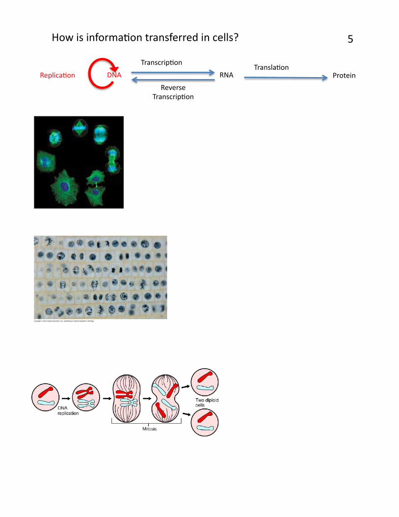
How is informaPon transferred in cells? 5

DNA Protein RNA
TranscripPon TranslaPon
ReplicaPon
Reverse TranscripPon
6
DNA Protein RNA
TranscripPon TranslaPon
ReplicaPon
Reverse TranscripPon
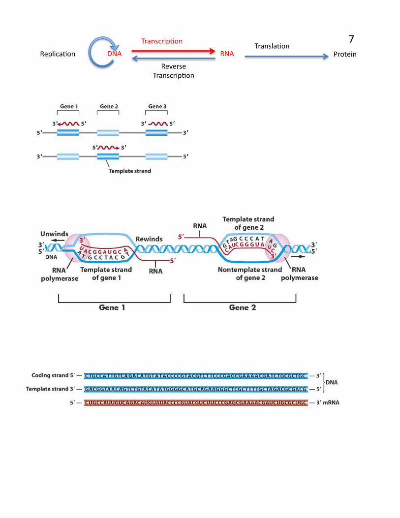
7

DNA Protein RNA
TranscripPon TranslaPon
ReplicaPon
Reverse TranscripPon
8

DNA Protein RNA
TranscripPon TranslaPon
ReplicaPon
Reverse TranscripPon
Translate this mRNA sequence AUG GAA CUA GUA AUC UCU AUU UCG GAU GAG GCG GAU UGA
9

DNA Protein RNA
TranscripPon TranslaPon
ReplicaPon
Reverse TranscripPon
PuXng it all together….
DNA Protein RNA TranscripPon
TranslaPon ReplicaPo
Reverse TranscripPon
Gene
Inside of cell
Polypeptide
Pre-mRNA
mRNA
DNA
Ribosome
Transcription completed
Processing
Transcription
Nucleus
Translation
10

What are the components of a gene?
Exon Intron Promoter
11

What are the components of a mRNA? How is mRNA processed from pre-‐mRNA?
Splicing
TranscripPon
Cap and poly-‐A addiPon
Genomic DNA
pre-‐mRNA
Spliced pre-‐mRNA
7-‐methyl-‐G-‐Cap AAAAAAAA mRNA
12

DNA Exon 3
3ʹ′ 5ʹ′
3ʹ′ 5ʹ′
Splice sites Start codon
Pre-mRNA
Exon 2 Intron 2
Intron 1
Exon 1
mRNA
Promoter
5′ 3′
Stop codon Terminator
What are the components of a mRNA? How is mRNA processed from pre-‐mRNA?
Details of pre-‐mRNA and mRNA
13

15 15
Experiment I: Analysis of the Actin gene of maize. You will use the actin gene to investigate the differences between the DNA gene sequence and mRNA sequence. This exercise will also demonstrate how gene structure (exon and introns) is determined experimentally. The process is one step in genome annotation or giving meaning to the billions of nucleotides that make up a genome. The actin gene encodes the actin protein and is found in all eukaryotes. Actin polymerizes to forms long strands that can contract and plays a large role in cell division. Because the role of actin is so important the chromosomal location of the gene is known in many organisms. This makes it a great gene to use for learning about gene structure and as a control for many experiments. While planning an experiment it is important to research what is already know about the subject. To do this you need to do literature search. Fortunately for a biologist this does not mean going to the library! We simply go online to the National Center for Biotechnology Information (NCBI) that is a unit of the National Library of Medicine (NLM) which is an institute in the National Institutes of Health (NIH) all funded by the US government. Using the NCBI Website The NCBI website is a portal for a lot of information including a literature reference (PubMed), a repository for free journal articles (PubMed Central), repository for DNA (GenBank) and protein sequences, and well as databases for the general public (DailyMed and MedlinePlus). The site also provides tools for accessing the information in many ways. Throughout Experiment 1 you will learn parts of the NCBI website.

16 16
To do a literature search 1. Go to www.ncbi.nlm.nih.gov to open the NCBI website. The page (currently) looks like this:
2. Click on the PubMed link (circled in red above). The PubMed homepage (currently) looks like this:

17 17
3. Type actin in the search box and click Search. Parts of this page will be explained in class.
As you can see there are over 70,000 articles that mention actin. Scroll down the page until you see a box on the right side called Search Details. There you will see the actual search used by PubMed: "actins"[MeSH Terms] OR "actins"[All Fields] OR "actin"[All Fields]. If a search does not produce what you expect it is a good idea to look at the Search Details to see what PubMed actually used. 4. We need to narrow the search so let’s try “actin and maize.” Now there are less than 200 articles.

18 18
5. Click on the link of the first article. On this page you will see the abstract of the article as well as related articles. This is often the most useful way to find articles that you are really interested in.
6. On the upper right hand side you will see and icon for the journal’s webpage were you can download the article. While PubMed (and everything on the NCBI website) is freely available everywhere you may have to be on UGA’s campus network to access the actual article. If the article is also in PubMed Central then you can download the full article from any Internet connection. A PubMed Central icon will appear next to the journal’s icon if the article is in the NCBI database. Since actin is found in all eukaryotes you might be interested to find out whether actin is associated with any diseases of animals or humans. NCBI has two hand curated databases that contain such information. To search for human diseases you use OMIM or Online Medalian Inheritance in Man and for animals you use OMIA.

19 19
7. Type actin into the search field and select OMIM from the pop up menu. Click Search.
The results of the OMIM search will look similar to this. We will discuss the OMIM page in class. Also you can do a similar search with OMIA.
As you can easily see, NCBI and PubMed make it possible to do all the background research you need for a biomedical and most plant topics without leaving the comfort of your own bed. Imagine how useful this would be writing a paper for class or researching a disease for medical school! A word of caution about NCBI: You may have noticed that the look and feel of the NCBI website changes depending on the database you are using. The home page and PubMed recently got a face lift. The other sections of NCBI will in time get the same treatment. So while the screen shots in the these pages may change, the basics of finding information on NCBI will remain the same.

20 20
Back to the Experiment… You will analyze the sequence of the maize actin genomic region and the actin mRNA sequence. What differences do you expect to find? The sequence of mRNA cannot be determined directly because there are no convenient techniques to determine RNA sequence. Instead, DNA is synthesized from RNA templates. This is done by using an enzyme called reverse transcriptase (RT for short) that catalyzes the synthesis of DNA from RNA (called reverse transcription, can you guess why?). DNA synthesized in this way is called complementary DNA or cDNA. cDNA synthesis is described in detail below. To obtain the sequence of a molecule of DNA you must first create sufficient quantities of just the region you are interested in. To do this you use a technique called the Polymerase Chain Reaction (PCR). Once you have enough DNA for sequencing it will be shipped off to a company called Genewiz that will sequence the DNA. You can then compare the sequences of the genomic DNA and the cDNA to determine the gene structure and compare that to the structure predicted in the fully sequenced maize genome.

21 21
Polymerase Chain Reaction. Better known by its initials - PCR: a technique enabling multiple copies to be made of sections of DNA molecules. It allows isolation and amplification of such sections from large heterogeneous mixtures of DNA such as whole chromosomes and has many diagnostic applications, for example in detecting genetic mutations and viral infections. The technique has revolutionized many areas of molecular biology—and won a Nobel Prize for Kary Mullis. The reaction starts with a double-stranded DNA fragment. A part of it is to be amplified (see Figure 1). Denaturation: A to B. The two DNA strands are separated (denatured) by heating to 95ºCelsius (C). Annealing: B. After cooling, short oligonucleotide primers (see below) that are complementary to the ends of the region to be amplified anneal with each strand. Extension: C. When the temperature is raised to 72º C the DNA polymerase (the heat-stable Taq polymerase) begins to catalyze DNA synthesis from the ends of the primer using the denatured DNA as template (the extension
Figure 1: Details of PCR. See below.

22 22
phase) and the nucleotide triphosphates (A, G, C, and T –collectively called dNTPs for deoxyNTPs) that are in the test tube. D,E and F - The procedure is repeated (for many cycles) beginning with denaturation then annealing, extension etc. Oligonucleotide primer. A primer is a short nucleic acid strand that serves as a starting point for DNA replication. A primer is required because most DNA polymerases (enzymes that catalyze the replication of DNA), cannot copy one strand into another from scratch, but can only add to an existing strand of nucleotides. (Recall from your lecture courses that in most natural DNA replication, the ultimate primer for DNA synthesis is a short strand of RNA. This RNA is produced by primase, and is later removed and replaced with DNA by a DNA polymerase.) The primers used for PCR are usually short, chemically synthesized DNA molecules with a length of about 20-30 nucleotides.
Denaturation: separation of the two DNA strands of a double helix by heating them to a very high temperature. This breaks the hydrogen bonds holding the double helix together.
Annealing: when DNA or RNA strands pair by hydrogen bonds to complementary strands, forming a double-stranded molecule. The term is also used to describe the reformation (renaturation) of complementary strands that were separated by heat.
Extension: enzymatically extending the primer sequence—copying DNA.
Watch this animation to help you understand how PCR works: http://www.dnalc.org/ddnalc/resources/pcr.html The PCR products are analyzed by gel electrophoresis. Watch this animation to learn how this technique works. http://www.dnalc.org/ddnalc/resources/electrophoresis.html

23 23
cDNA Synthesis The polymerases used for PCR require a DNA template. That means we cannot use mRNA directly in a PCR reaction. We must extract RNA from a tissue and reverse transcribe the RNA into DNA using the enzyme reverse transcriptase (RT). RT creates the DNA complement of every mRNA strand in the reaction. This DNA strand is referred to as cDNA. cDNA can then be used in a PCR sample as the template for Taq polymerase. cDNA is made from mRNA using RT, dNTPs, and a primer that binds to the poly-A tail of the mRNA. The DNA primer is a short DNA strand that is fifteen T bases in a row and is called oligo-dT. The oligo-dT primer binds to the poly-A tail and the RT extends the oligo-dT primer to create a strand of DNA that is complementary to the mRNA strand. Due to time constraints you will not isolate RNA and make cDNA for this first experiment. Instead you will perform two different PCRs – (i) you isolate maize genomic DNA in class and, using specific primers, amplify the actin gene and (ii) you will amplify the actin cDNA from cDNA made by the instructors. You will then analyze the sizes of the PCR products from (i) and (ii). Finally, you will analyze the sequence of the PCR products to determine the exon/intron boundaries of the first intron of the actin gene. This will provide you with an example of how the gene structure of any gene can and often is determined.

24 24
Step I: DNA Extraction You will extract DNA from two maize strains: B73 the reference strain and another imbred. Be sure to store the DNA in the freezer because you will use it through out the semester. This protocol should be written up in your lab notebook. You will use your lab notebook in lab, not the printed course book.
Damon Lisch’s All Natural Genomic Miniprep Materials list: Extraction Buffer RNase A (500µg/ml) 10% SDS 5M KOAC 100% Isopropanol 70% Ethanol Ice Bucket with ice liquid nitrogen 37˚C water bath 65˚C water bath sterile 1.5 ml tubes (2 for each prep) 1) Label 2 tubes for each plant with plant name and your initials. 2) Harvest a piece of maize leaf about the length of your hand. Rip it into pieces small enough to fit in the mortar. Ask for liquid nitrogen to be put in the mortar. Grind vigorously with the pestle. 3) Add 1 ml of Extraction Buffer, and grind some more in the buffer. Pour the slurry into the appropriately labeled tube. 4) Add 8.0 µl RNase A to the tube. Use only the pipette labeled for RNase A use. Incubate for 15 minutes at 37˚C. RNase A is an enzyme that degrades RNA strands into single bases. Repeat steps 1-4 for the next sample. 5) Add 120 µl of 10% SDS. Mix by inverting.

25 25
6) Incubate at 65˚C for 10 minutes. 7) Add 300 µl 5M KOAc. Mix well by inverting several times (important!), then incubate on ice for 10 minutes. 8) Spin for 5 minutes at top speed in microfuge. Squirt 700 µl of the supernatant through miracloth into the second tube. (make small funnel, place tip directly onto the miracloth at the tip of the funnel and squirt through – do not allow the whole funnel to get soaked). 9) Add 600 µl of isopropanol. Mix the contents thoroughly by inverting. DNA precipitate may or may not be visible at this point; don’t worry if you don't see much. However, a really good prep (excellent grinding of tissue) should result in visible DNA at this stage. 10) Spin for 5 minutes at top speed. Pipette off supernatant. 11) Add 500 ul of 70% ethanol and flick until the pellet comes off the bottom (for best washing results). Spin 3 min, then pipette off the ethanol with a P-1000. Suck off the rest of the ethanol with a P-20 pipette. Make sure the pellet stays in the tube! Let air dry in hood for about 5 minutes with the caps open. 12) Resuspend the DNA in 50 µl water. Store your DNA samples in a box with your name the freezer (-20˚C). Visualize genomic DNA on a 1.5% agarose gel: A 1.5% agarose gel contains 1.5 grams in 100 ml of gel buffer TAE (1.5/100 x 100% = 1.5%). 1. Weigh out 1.5g agarose and add to a 250 ml flask.
2. Add 100 ml 1X TAE buffer (available in a big jug) to the flask with agarose. (TAE = 40mM Tris acetate, 1mM EDTA pH 8.4)

26 26
3. Heat contents in the microwave until boiling (2-3 min). Be very careful, as superheated liquids can boil over and burn you.
4. Swirl to make sure that the agarose is completely melted. 5. Add 1.0 µl of a stock solution of 100 mg/ml ethidium bromide (EtBr). (This binds to the DNA allowing it to be visualized under UV light. Do not let this stuff touch your skin.)
6. Swirl again to mix and pour into a gel-casting stand with a comb (this will be demonstrated in the lab.) The gel should cool and solidify within 10-15 minutes at which time it is ready to place the gel in the electrophoresis apparatus and add enough TAE buffer to completely immerse the gel. After the gel solidifies 7) Put 10 µl of DNA into a tube. 8) Add 2 µl of 6x loading dye (blue dye) to the tube. Tap the tube gently with your finger to mix. 9) Load all 12µl on your gel. Keep track of which sample went in which lane. 10) Load 7 µl of DNA Ladder in one empty well. 11) Run the gel at 130 Volts for 30 minutes. 12) Photograph the gel. Determine the DNA concentration DNA concentration is determined by measuring the amount of UV light (260 nm) absorbed by the DNA. The absorbance is converted into concentration by using the relationship that an absorbance reading of 1 corresponds to a concentration of 50 µg/ml of pure DNA. So a solution of DNA that has an absorbance of A260 = 0.5 has a concentration of 25 µg/ml (50 X 0.5=25). What is the concentration in µg/µl and ng/µl?

27 27
Other molecules also absorb at 260 nm and inflate the DNA concentration value. You can also use the Nanodrop spectrometer to determine the purity of the DNA solution by taking readings at 280 (protein) 230 (EDTA, carbohydrates, and phenol) and 320 (this is visible light and measures particulates). Purity is determined by taking the ratio of the A260 value to the A280 or A320. A260/280 ratio for pure DNA is 1.8. Your values should be between 1.7 and 2. The A260/A320 ratio for pure DNA is between 2.0 and 2.2. The Nanodrop spectrophotometer will scan the DNA sample from 200 nm to 400 nm and report values for A230, 260, 280, 320, the concentration, and ratios. You must record these numbers in your notebook. You will be shown how to use the Nanodrop in class. Dilute the DNA sample You need to add between 50 and 100 ng of DNA into each PCR. You will most likely need to dilute your DNA sample. A good concentration to use is 20 ng/µl. Calculating dilutions is an important skill that you need to know for lab. You should remember from chemistry that a dilution is made using the formula civi=cfvf. In biology lab we re-arrange the equation like this: Final concentration (cf) X Final volume (vf) = Volume of stock (ci) Stock concentration (ci) So if you have a DNA concentration of 500 ng/µl and you want to make 100 µl of solution that is 20 ng/µl you set up the formula this way 20 ng/µl X 100µl = 4 µl 500 ng/µl In a labeled tube you would place 96 µl of sterile water and 4 µl of the concentrated DNA solution. How many microliters of the diluted DNA do you need for 50 ng?

28 28
Step II: Amplify DNA using PCR. Each person will perform PCR using as template the B73 genomic DNA and one inbred line you isolated in class and the cDNA provided by the instructor. We also need an additional negative control that will be water in place of DNA, giving you five reactions. Instead of mixing the PCR reagents separately for each reaction we first make a cocktail of all reagents in common (Taq, dNTPs, Primers, and water). To ensure we have enough cocktail for five reactions we add one extra. Set up PCR 1) Label a 1.5 ml tube. This is for making the PCR mix. 2) Label a strip of 0.2 ml PCR tubes. The instructors will show you where to label the tubes. The label may be rubbed off in the machine if you put it in the wrong place. 3) Mix the following in your tube using the volumes in the column labeled x4. Keep this on ice. You will need to calculate the number of µl of DNA to add and then adjust the volume of water. x1 (µl) X6 2x Master Mix 25.0 H2O Forward Primer 1.0 Reverse Primer 1.0 DNA 100 ng -‐-‐-‐-‐-‐-‐ Total 50.0 The 2x Master Mix is supplied by a company (NEB) and contains Taq enzyme, buffer, and deoxynucleotide triphosphates (dNTPs) in a 2x concentration. This means that it must be diluted by half for the working concentration (1x). This tube should be kept on ice to protect the enzyme from degradation. 4) Put 45.0 µl of master mix in 5 of the PCR tubes. 5) Add the DNA to the PCR tubes. Add 5 µl of sterile water in tube 5.

29 29
6) Seal the tubes tightly with a strip of caps. Keep PCR tubes on ice until everyone is finished. After everyone is done, your samples will be placed in a thermocycler or ‘PCR machine’ and cycled with the following conditions:
1 cycle for: initial denaturation 94°C 3 min 40 cycles for: denaturation 94°C 30 sec
annealing 50°C 30 sec extension 72°C 1 min
[Note: “40 cycles” means all steps— denaturation, annealing, and extension—are repeated 40 times before going on to the next step] 1 cycle for: final extension: 72°C 10 minutes
7. After you finished setting up the PCR, you should pour a 1.5% agarose gel. See page 20-21. You will pour one gel per group. Step III. Gel analysis. 1. Pipette 20 µl of each PCR reaction into a new tube. Add 4 µl loading dye. Load 20µl into a gel lane. Remember to add a lane with 7 µl of DNA ladder. Run the gel at 130 V for 30 minutes. The sizes of the DNA bands in the ladder are shown in the figure below.

30 30
Step IV. Prepare samples for sequencing If there is only one band in a lane, the PCR sample can be used for sequencing after an enzymatic cleanup. Two enzymes are used: Exonuclease I that degrades the primers to single nucleotides and shrimp alkaline phosphatase that removes the phosphate group from unincorporated dNTPs. The mix is called ExoSAP-IT. Keep the ExoSAP-IT on ice. 1. Label a 1.5 ml tube and put 10 µl PCR product in the tube. 2. Add 4.0 µl of ExoSAP-IT reagent. 3. Incubate 37˚C for 15 min. then 80˚ for 15 min. 4. Prepare the sample for sequencing. Instructions will be given in class.
How your DNA samples will be sequenced DNA sequencing is the process of determining the nucleotide order of a given DNA fragment. Most DNA sequencing is currently being performed using the chain termination method developed by Frederick Sanger. [Sanger is particularly notable as the only person to win two Nobel prizes in chemistry - his second in 1980 for developing this DNA sequencing method and his first in 1958 for determining the first amino acid sequence of a protein (insulin)]. His technique involves the synthesis of copies of your input DNA by the enzyme DNA polymerase. However, one difference between this reaction and PCR, for example, is the use of modified nucleotide substrates (in addition to the normal nucleotides), which cause synthesis to stop whenever they are incorporated. Hence the name: “chain termination”. Chain terminator sequencing (Sanger sequencing) Your samples were sent to Genewiz along with information about the sequencing primer to be used (recall that DNA polymerase needs a primer to start DNA synthesis of a template strand). The reaction contains your DNA sample, the sequencing primer, DNA polymerase and a mixture of the 4 deoxynucleotides that are “spiked” with a small amount of a chain terminating nucleotide (also called dideoxy nucleotides, see below).

31 31
Limited incorporation of the chain terminating nucleotide by the DNA polymerase results in a series of related DNA fragments that are terminated only at positions where that particular nucleotide is used.
The fragments are then size-separated by electrophoresis in a slab polyacrylamide gel, or more commonly now, in a narrow glass tube (capillary) filled with a viscous polymer.
Figure 2. A chain-terminating nucleotide triphosphate (called a di-deoxynucleotide or ddNTP). Because it has a “H” instead of a “OH” at the 3’ position, it is not a substrate for the addition of another NTP and DNA synthesis terminates.

32 32
Modifying DNA sequencing to automation: dye terminator sequencing (this is how your DNA samples will be sequenced) An alternative to the labeling of the primer is to label the dideoxy nucleotides instead, commonly called 'dye terminator sequencing'. The major advantage of this approach is the complete sequencing set can be performed in a single reaction, rather than the four needed with the labeled-primer approach. This is accomplished by labeling each of the dideoxynucleotide chain-terminators with a separate fluorescent dye, which fluoresces at a different wavelength.
Figure 3. DNA is efficiently sequenced by including dideoxynucleotides among the nucleotides used to copy a DNA segment. (a) In this example, a labeled primer (designed from the flanking vector sequence) is used to initiate DNA synthesis. The addition of four different dideoxynucleotides (ddATP is shown here) randomly arrests synthesis. (b) The resulting fragments are separated electrophoretically and subjected to autoradiography. The inferred sequence is shown at the right. (c) Sanger sequencing gel.

33 33
Figure 4: DNA fragments can be labeled by using a radioactive or fluorescent tag on the primer (1), in the new DNA strand with a labeled dNTP, or with a labeled ddNTP.
Figure 6: Sequence ladder by radioactive sequencing compared to fluorescent peaks
Figure 5. Modern automated DNA sequencing instruments (DNA sequencers) can sequence up to 384 fluorescently labelled samples in a single batch (run) and perform as many as 24 runs a day. However, automated DNA sequencers carry out only DNA size separation by capillary electrophoresis, detection and recording of dye fluorescence, and data output as fluorescent peak trace chromatograms.

34 34
This method is now used for the vast majority of sequencing reactions, as it is both simpler and cheaper. The major reason for this is that the primers do not have to be separately labeled (which can be a significant expense for a single-use custom primer), although this is less of a concern with frequently used 'universal' primers.
Figure 7. An example of a chromatogram file of a Sanger sequencing read. The four bases are detected using different fluorescent labels. These are detected and represented as 'peaks' of different colors, which can then be interpreted to determine the base sequence, shown at the top.

35
Step V. Sequence Analysis. Now that you have DNA sequence from the PCR bands you need to analyze that sequence. We will do the following analyses: I. Verify the sequences are from the actin gene – Page 40. Bioinformatics technique: blastn II. Compare the two sequences to each other – Page 44. Bioinformatics technique: blast2sequences III. Compare the sequences to the maize genome – Page 49. Bioinformatics technique: Genome Browsers IV. Compare the class generated sequences to each other – Page 59. Bioinformatics technique: Multiple Sequence Alignment V. Find related sequences in the maize genome and other organisms – Page 72. Bioinformatics technique: protein blast, tblastn, TARGeT Before we analyze the sequence we need to obtain the sequence and also we need to create a way to document the annotation you are doing. Obtain sequences from Genewiz Website. Before you can analyze sequence you must obtain the sequence from the Genewiz website and check the quality. 1. Open the Genewiz website and login in: https://clims3.genewiz.com/default.aspx user: [email protected] password: 1503A

36
2. Click the tracking number provided in class.
3. Find your samples on the spreadsheet. I will explain the naming in class. 4. Find a sample were the QS (for quality score) and CRL (contiguous read length) are both in black. These numbers help you assess the quality of the sequence. We will discuss this in class. 5. Click on “View” in the Trace File column.
6. A new window will pop up. On the top will be the trace file and on the bottom will be the sequence. We will discuss how the trace file is used to assess the quality of the sequence.

37
Documenting your annotation efforts It is just as important to maintain a notebook record of sequence annotation as it is to maintain a lab notebook. Because most annotation is done on the computer a paper notebook is not very useful. In this class you will be required to use Google Docs (docs.google.com) for annotation. This is a convenient method and you can work easily in the classroom or at home. Also when it is time to turn in an assignment you will just “Share” it with the instructors. If you do not have a Google Docs account create one before you come to class. It’s free. You should keep a logical record of what you do during sequence analysis and include your thoughts and ideas as you work. For each step in the analysis you should record any query sequences, results and screen shots of the results. There should be enough information so that you could easily repeat what you did. Here are some helpful hints for using Google Docs and keeping an online notebook: 1. On a Mac you can take a screen shot by using “Command+Shift+4.” The “Command” keys are on each side of the spacebar. 2. On a Mac you can drag and drop images from a browser to the desktop. 3. In the Maize Browser there is an “Export Image” button on the lower right of most image boxes. Click it and a contextual menu will appear. Select “Export PNG” from the list. 4. Format DNA and Protein sequences using Courier Font size 9.

38
5. DNA and Protein sequence should be in FASTA format with the first line starting with “>” and containing the name of the image. The remaining lines are the sequence in fixed length. To clean up sequence use this web tool: target.iplantcollaborative.org/fasta_formatter.html. This tool is also useful if you need a subsequence from a longer sequence. I. Verify the sequences are from the actin gene PCR is a very useful technique, but sometimes it generates artifacts, that is random sequences unrelated to the sequence of interest. We first want to make sure that the sequence from the PCR bands is what we want to study. There are several ways to do this, but we will use Blast from NCBI to analyze the sequence. Introduction to Blast: You will use Blast a lot this semester. It is the major biological sequence search tool for DNA, RNA, and protein databases. Whole genomes can be searched using Blast. Access Blast by clicking on the Blast link on the NCBI home page (http://www.ncbi.nlm.nih.gov/).
The Blast link will take you to the Blast page and to the Basic Blast Menu which will also be used frequently in this course:

39
There are six different versions of BLAST because you can use a nucleotide sequence or protein sequence to query nucleotide or protein databases. The different versions are summarized in the screenshot above. Today we will give nucleotide blast a test drive. We will discuss protein blast and tblastn later when we need to use them.
A. Nucleotide Blast: This is the most straightforward type of search. You begin with a nucleotide sequence you want to know more about (the query) and “blast” it against a nucleotide database (the subject).
You can learn a lot about your query sequence with a blast including: a. Are there publications that already report information about
this sequence (have you been “scooped”)? b. Where is the sequence located in the genome (more on location
in class)? c. Is the sequence found in genomes of closely related organisms? d. Does it code for an RNA and/or a protein? If so is anything
known about its function?

40
1. Select ‘nucleotide blast.’ Cut and paste the following sequence in the Query text window (Enter accession number….). For the in class example we will use the actin genomic DNA sequence. You can use this sequence or your sequence.
>Actin Genomic Sequence GTGACAATGGCACTGGAATGGTCAAGGTTGTTATCTCGTTCAGAAGTCTTTTTCAACAAA GCAACTCTACTCCTGTGCCTAATTGTTGCTCAACTCCTCAATATTTACAGGCCGGTTTCG CTGGTGATGATGCGCCAAGAGCTGTCTTCCCCAGCATTGTGGGAAGACCACGCCACACCG GTGTCATGGTCGGCATGGGCCAAAAGGATGCCTACGTAGGTGATGAGGCTCAGGCCAAGA GAGGCATCCTGACACTGAAGTACCCGATTGAGCATGGCATTGTCAACAACTGGGATGACA TGGAGAACTGGCATCACAC
2. Under “Choose Search Set” select “Others” and the drop down list changes to “Nucleotide Collection (nr/nt).” This is the complete non-redundant nucleotide database.

41
3. The next section gives you three options for a nucleotide blast.
Choose megablast (default) .
4. Select the “Blast” button. What you see below is called the queue page:
5. When your search is complete a results page will be presented. We will discuss this page in detail in class.

42
6. Details of the Alignment (to be discussed in class)
A short discussion on how Blast works. Blast takes the query sequence and divides it into “words” based on the word size parameter (the default is usually “fine”). For a megablast query the default (and minimum) is a size of 28. The algorithm then takes these “words” and runs them against a hash database where the large database is cut into 28 bp words. When an exact match occurs, the program attempts to extend the alignment in each direction on the full sequence. If the alignment extends then a score is calculated and as long as the score remains above a threshold the alignment continues. If a mismatch occurs the score decreases, but as long as the score remains above threshold the mismatch is allowed. Word size can be changed. Long word sizes increase stringency. The threshold is determined by the Expect value in the “Algorithm Parameters” tab on the Blast page. The default Expect value is 10. This means that you expect to find 10 matches to your query in randomly generated sequence. Blast uses this value, the size of the query sequence, and the size of the database (called the search space) to calculate a threshold on 10 random matches and then reports only hits that score

43
better than the random model. Lowering the Expect value increases the stringency of the search. While extending the alignment Blast may encounter a series of mismatched nucleotides. Blast will try to skip over the mismatch region (called opening a gap) to see if the alignment begins again. If the alignment begins again, Blast will continue. If the alignment does not begin again, the alignment process stops and Blast reports the hit. Opening a gap is penalized heavily. Extending a gap is also penalized. The process of opening gaps is necessary to allow for small insertion mutations that occur fairly frequently in a genome.

44
II. Compare the cDNA to the genomic DNA sequences. We need to line up the two sequences to determine where they are similar and where they differ. We could do this by hand for short PCR sequences, but it would be very time consuming. Computer programs are very good at this type of analysis and are extremely fast. We will modified version of blastn called Blast2Sequences. 1. Open a web browser and go to the Blast Website (http://www.ncbi.nlm.nih.gov/blast/Blast.cgi) and click on the ‘nucleotide blast’ link.
2. Check the ‘Align two or more sequences’ checkbox.

45
3. A) Enter the ‘Actin Genomic DNA sequence’ in the Query (top) textbox and B) the Subject (bottom) ‘Actin cDNA sequence’ in the bottom text box. C) Click ‘Blast.’
4. The results. In the top half of the page the results are presented diagrammatically. The query is shown as a red, thick rectangle. Any similarity between the query and the subject is shown as thin rectangles below the query. The color of the rectangle indicates the hit score. The higher the score the better the hit. The Query is the Genomic DNA sequence and the Subject is the cDNA sequence. In this case there are two hits between the query and the subject. What do these hits represent?
A.
B.
C.

46
The bottom half of the results page shows the two hits nucleotide-by-nucleotide called alignments. When bases at the same position are the same a vertical line is placed between them. The alignments are ordered by score from highest to lowest. Notice that the second alignment starts with 1 in both query (genomic DNA) and subject (cDNA) while the first alignment starts at nucleotide 161 in the query and 78 in the subject.

47
So the cDNA sequence matches the genomic DNA from nucleotides 1 to 78 and then from nucleotides 161 to 371. 1. What do these two alignments represent? 2. What is the sequence from 79 to 160 in the genomic DNA? Why isn’t this sequence present in the cDNA?

49
III. Finding the Actin gene in the Maize Genome Now that you have verified that the sequences you have are from the actin gene you need to compare the sequence to the published maize genome sequence. To do this we will use blast and the maize browser. The B73 strain of maize was sequenced to high quality. This is now considered the reference genome for all maize genomic work. The genomes of two other maize strains Mo17 and Palomero (a popcorn) have also been sequenced but not to the level of quality of B73. You will start exploring a genome by finding the location of actin in the maize genome. Genome sequencing is an involved process. Read pages 453-468 of Chapter 13 from Introduction to Genetic Analysis. This can be downloaded from the course web page. “BLASTing” the Maize Genome While the blast programs were written by scientists at NCBI, the programs are freely available and are used by many DNA sequence repositories. For the maize browser we use blast to find the location of our sequences on the maize chromosomes. 1. Open the maize browser (www.maizesequence.org). The home page contains information about the B73 genomic sequence. You should read this page and the information pages to learn more about the sequence and the tools that are available on the website. For now, click on BLAST in the upper right hand corner.

50
2. Paste your genomic DNA sequence in the textbox. This is your query. We are using the programs with all defaults so click “Run.”

51
3.The blast results are show three ways: A) By karyotype (chromosome)
B) Alignment by query (similar to what you see on the NCBI results page)
C. Alignment summary.

52
The Alignment Summary is the most useful of these windows. Usually the summary will look similar to this, but from time to time you may need to use the menus to turn on various columns of information. For this query we want to look at the one that has the higest %ID or the lowest E-val. As you can see the first row of the results is 98.45% and is located on Chromosome 8. The percent match of your sequence may be different but it should still be on chromosome 8. The 4 letters on the left are links to useful information: [A] – This link will take you to the alignment. Click on this link to see why the sequence is only a 98.45% match and not 100%. [S] – This is the sequence of the query. [G] – This link will take you to the genomic sequence. This is where you can download the B73 sequence that matches your sequence.
[C] – This link takes you to the Contig viewer that is explained it detail below. Click on the [C] now. Maize Genome Browser The maize genome is very large and has many features: genes, simple repeats (CACACACA or TTATTATTATTA, etc.), transposable elements, ESTs (similar to cDNA), and many other things. Genome browsers were developed to visualize all of the features of a region of the genome in a single window. Many of the features can be clicked on for coordinates and detailed information. We will be using the 4a.53 version of the B73 sequence. The browser is a bit clunky at times so just ask questions if the browser on your screen does not match the browser on paper. The figure below shows the region of the maize genome that contains the actin gene. This is called the “Contig View.” There is a lot of information on this figure. We will discuss most of it in class.
53
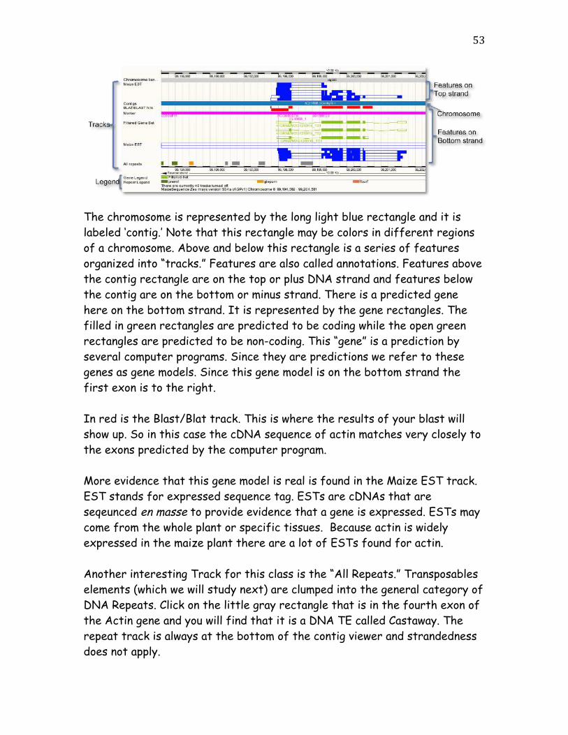
The chromosome is represented by the long light blue rectangle and it is labeled ‘contig.’ Note that this rectangle may be colors in different regions of a chromosome. Above and below this rectangle is a series of features organized into “tracks.” Features are also called annotations. Features above the contig rectangle are on the top or plus DNA strand and features below the contig are on the bottom or minus strand. There is a predicted gene here on the bottom strand. It is represented by the gene rectangles. The filled in green rectangles are predicted to be coding while the open green rectangles are predicted to be non-coding. This “gene” is a prediction by several computer programs. Since they are predictions we refer to these genes as gene models. Since this gene model is on the bottom strand the first exon is to the right. In red is the Blast/Blat track. This is where the results of your blast will show up. So in this case the cDNA sequence of actin matches very closely to the exons predicted by the computer program. More evidence that this gene model is real is found in the Maize EST track. EST stands for expressed sequence tag. ESTs are cDNAs that are seqeunced en masse to provide evidence that a gene is expressed. ESTs may come from the whole plant or specific tissues. Because actin is widely expressed in the maize plant there are a lot of ESTs found for actin. Another interesting Track for this class is the “All Repeats.” Transposables elements (which we will study next) are clumped into the general category of DNA Repeats. Click on the little gray rectangle that is in the fourth exon of the Actin gene and you will find that it is a DNA TE called Castaway. The repeat track is always at the bottom of the contig viewer and strandedness does not apply.

54
Instructions for controlling visible tracks are found at the end of this chapter pages 52-53. Drilling down for more information Each track in the contig view has supporting information that you can obtain. In this example you will find the genomic coordinates for the exons of the actin gene. 1. Click on one of the gene models in the Contig Viewer. A contextual menu will appear. Click on the gene number (GRMZM2G…).

55
2. Some details about the gene model will appear in a new tab. To get exon information click on one of the Transcript IDs.
3. A new tab will open. On the left is a menu list. Click on the General Identifiers under “External Information” heading. Here you will see EST and other evidence that suggests that this is the maize Actin 1 gene.
Tab Row

56
4. Click on “Exons” in the left menu bar. The exons with sequence will appear. Note that the exons are ordered from 5’ to 3’ (that is exon 1 is listed first) but the genomic start and stop numbers are running backward. Also note that the sequence shown on the right is the sequence of the Actin 1 gene, not the reverse complement.
You should record the exon locations in your Google Doc. How would you obtain the protein sequence? Your homework assignment is to compare the cDNA sequence you obtained and the remainder of the sequence on the class website to the maize browser. Do the predicted exons in the gene model match the experimental evidence?

57
Appendix: Adding and removing tracks from the Contig Browser. Currently there are over 30 tracks of information available for viewing in the browser. To select which tracks are visible use the “Configure this Page” link in the left hand menu bar.
An overlay window will appear and you can select the categories of tracks in the left hand menu bar. Most categories will have several sub-categories. Select what you want on or off and then click the Save and Close button in the upper right of the window. The Contig Browser with reload with the new selections. You may want to register for an account as this may remember your settings. This is not a guaranteed behavior though. Register before you come to class. Write your user name and password on this page.

59
IV. Compare class sequences to each other. Everyone in the class sequenced a band from the reference strain B73 and from an inbred line or land race line. In early parts of the sequence analysis you should have noted any sequence polymorphisms between the B73 and the other strain you are working with. In this step we will look more carefully at the locations of the polymorphisms. A sequence polymorphism is any difference at the same DNA base or bases between two individuals of the same species. On common type difference is the single nucleotide polymorphism or SNP (pronounced “snip”). SNPs are most often caused by mistake made by DNA Polymerase during replication. Other types of polymorphisms include indels where sequence is inserted or deleted between two individuals. So far you have used blast to align a query sequence to one other sequence. In this case we need to align many sequences together at once this is called a multiple sequence alignment. There are two commonly used programs for multiple sequence alignment: ClustalX and MUSCLE. Both are available on the web for free. The first step in multiple sequence alignment is to do all pairwise alignments. Right away you can see that for a small number of sequences there is a lot of computation work to be done. After pairwise alignment the pairs are scored and then the multiple alignment is put together based on these scores. Often there is no one solution to a multiple alignment; ClustalX and MUSCLE may give slightly different results on the same sequences. Multiple sequence alignments are often edited by the researcher as well. Preparing sequences for multiple sequence alignment
1. All sequences need to be of similar lengths. One very short or very long sequence relative to the others will mess-up the alignment completely.
2. Use concise names for the sequences. Some multiple sequence alignment programs will truncate names.
3. Sequence should be in the multiple FASTA format. >Seq_1 AGCGTCAAGCTAGACGAC >Seq_2 AGGACGTACACCGACTGGACGGACTTG >Seq_3 AGCCTGCCGTTCGGCGA

60
Multiple Sequence Alignment using MUSCLE You can access MUSCLE from the EBI bioinformatics website www.ebi.ac.uk/Tools/muscle/index.html or from the TARGeT website: target.iplantcollaborative.org/class_index.php. The TARGeT website has a collection of tools that we will use in class. 1. Get all sequences into a single FASTA file. We will use a shared Google Doc to collect the sequences. Create a name for your sequence that has the inbred name first and then your initials, e.g., B73_JMB.

61
2. Open the TARGeT MUSCLE web page target.iplantcollaborative.org/class_index.php and click on “Multiple Sequence Alignment.” Copy and paste the sequences into the text window. Click “Align.” There are not very many parameters for a multiple sequence alignment program and you will almost always use the defaults.
3. The results are presented on the next page. The results are easy to read, but we will go over them in class.

62
The text output of the alignment program will put in a dash to represent gaps in the sequence. If all of the nucleotides are the same at a given position a ‘*’ will be placed below the alignment at that position. As you can see a multiple sequence alignment makes it very easy to find sequence polymorphisms.

63
4. Another way to view the sequence is using a program called Jalview. This viewer provides many ways to view the alignment.
In Jalview the sequences can be color coded in several different ways. Here they are colored by base. Jalview also creates a “Consensus” sequence where the most common nucleotide at each position is used. The bars above the consensus sequence indicate the degree of consensus. These bars also make it easy to scan for polymorphisms especially in alignments with many sequences. 5. Determine the position of the exons in the B73 sequence and “map” the polymorphisms to exon and intron. Where would you expect polymorphisms to be more frequent? Why? Were do the majority actually occur?

65
IV. Actin Gene Families So far we have been studying the actin 1 gene of maize, but there are several actin genes in the maize genome. Through the process of gene duplication and subsequent diversification one gene can give rise to many genes in the same genome. An example of a gene family from Making of the Fittest is the opsin genes. Using bioinformatics tools we can identify family members starting with actin 1 of maize. Before we can find gene families we must first learn about two other types of blast: protein blast (blastp) and translated nucleotide blast (tblastn). Protein Blast: A protein blast utilizes an amino acid sequence query from the user as the input and searches a protein database. This is often useful to determine whether the sequence already exists in the database or to predict the function of the predicted protein. The steps for submitting a query are similar to a nucleotide blast and the algorithm is essentially the same. There is one key difference in the protein vs. nucleotide algorithm. When a nucleotide is compared to a nucleotide only matches between the same bases are allowed (A->A, G->G, etc). In contrast, some amino acids have similar chemical properties. For example asparagine (asp) and glutamine (glu) have the same functional group with glutamine having a slightly longer side chain due to an extra methyl group. Asp and glu are often interchangeable without detriment to protein function. The figure below groups the amino acids by functionality.
(www.neb.com)

66
To score similar amino acid matches, blast uses a look-up table called a BLOSUM matrix. This table contains all possible amino acid matches and a score to use for each. The default matrix is BLOSUM62. Common groupings of the amino acids (from http://www.uky.edu/Classes/BIO/520/BIO520WWW/blosum62.htm):
G,A,V,L,I, M aliphatic (though some would not include G) S,T,C hydroxyl, sulfhydryl, polar N,Q amide side chains F,W,Y aromatic H,K,R basic D,E acidic
1. Open a protein blast from the blast home page (http://www.ncbi.nlm.nih.gov/blast/Blast.cgi), and choose protein blast. Copy-and-paste the actin protein sequence you obtained from the maize browser. (This should be in your notes!)
2. Run the Blast with all default parameters. The queue screen will report that it found a similarity between your query sequence and the Protein Family (PFam) database.
3. The results page is similar in organization to the nucleotide blast results page. Here is the first alignment reported. Note in this alignment that when two similar amino acids match a ‘+’ is used.

67
Translated Nucleotide Blast (tblastn) This type of blast takes a protein query sequence and blasts it against a nucleotide database. This is incredibly useful because: 1. it can find the location of the gene encoding the protein in a genome. 2. it can find similar sequences in the genome. 3. it can find similar sequences in related genomes. To search a nucleotide database with a protein query, the database must first be translated. NCBI stores the nucleotide databases translated in 6 frames. Why 6 frames? 1. Start at the Blast page and click on tblastn, the fourth choice down.

68
2. Enter the actin query sequence from your notes. Remember, this process compares a sequence of amino acids against sequences in existing genomes.
3. Now go down to the section called “Choose Search Set.”
4. For the first panel under “Choose Search Set,” leave it on the default setting, which is “Nucleotide collection (nr/nt)” nr: non-redundant, nt: nucleotide.
5. Go the bottom and click on BLAST! The Algorithm parameters are similar to the nucleotide blast and protein blast search. They serve the same functions here.
69
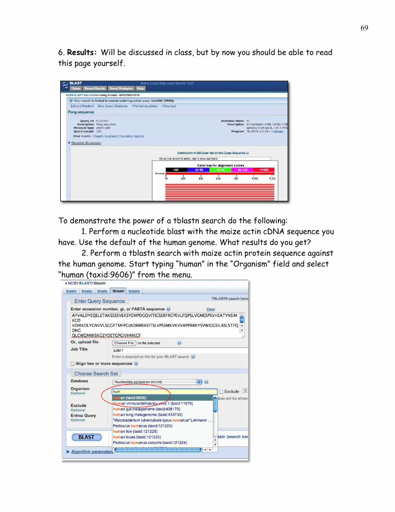
6. Results: Will be discussed in class, but by now you should be able to read this page yourself.
To demonstrate the power of a tblastn search do the following: 1. Perform a nucleotide blast with the maize actin cDNA sequence you have. Use the default of the human genome. What results do you get? 2. Perform a tblastn search with maize actin protein sequence against the human genome. Start typing “human” in the “Organism” field and select “human (taxid:9606)” from the menu.
70
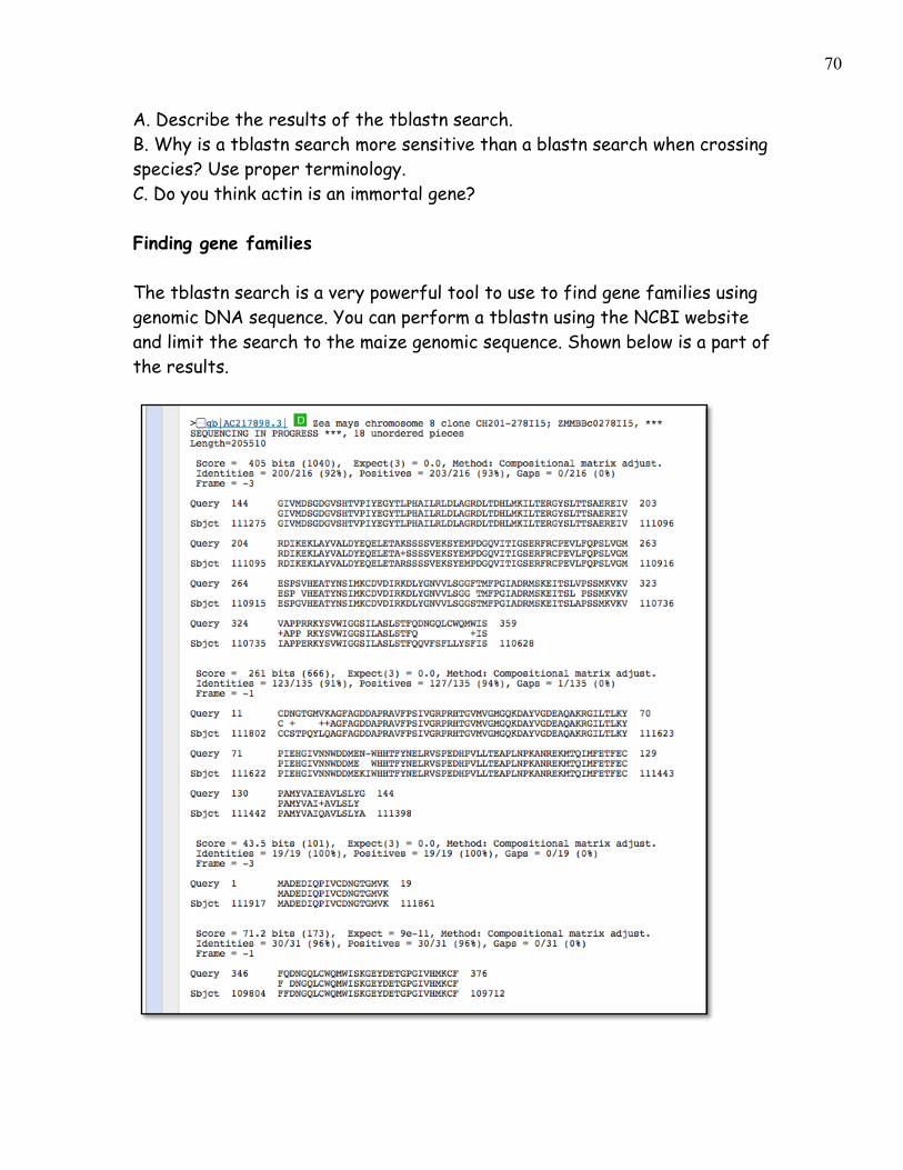
A. Describe the results of the tblastn search. B. Why is a tblastn search more sensitive than a blastn search when crossing species? Use proper terminology. C. Do you think actin is an immortal gene? Finding gene families The tblastn search is a very powerful tool to use to find gene families using genomic DNA sequence. You can perform a tblastn using the NCBI website and limit the search to the maize genomic sequence. Shown below is a part of the results.

71
In this example the protein query matched a region on Chromosome 8 of the maize genome, but the match is broken in to 4 pieces. These pieces represent the four coding exons of the actin 1 gene. (Note the coordinates are very different from the coordinates in the maize browser because NCBI uses a different version and format of the sequence.) By looking at the start and stop of each piece you can put together the gene structure of actin 1. You will notice that there is some overlap between the pieces so to fully create the actin gene you would need to edit the alignments by eye. So while it is possible to manually find gene family members, it is incredibly time consuming and tedious. Luckily we have computers to aid us! A very useful set of tools for identifying gene families was written by Yujun Han, a former TA of this class. Yujun is a graduate student in Dr. Wessler’s lab. This set of tools is called TARGeT for Tree Analysis of Related Genes and Transposons. TARGeT can use a blastn or tblastn to start the process of building gene families. Gene structures are extracted from the blast results in the second step called Putative Homolog Identification (PHI.) The results of PHI contain all the information about the homologs it found, but it is difficult for a human to determine which homologs are more or less related. To help show relationships between the homologs TARGeT also generates a type of phylogenetic tree called a gene tree. From this tree we can easily see which homologs are more closely related and make other predictions. A discussion on how trees are built and interpreted is found at the end of this lesson (page 77).
72
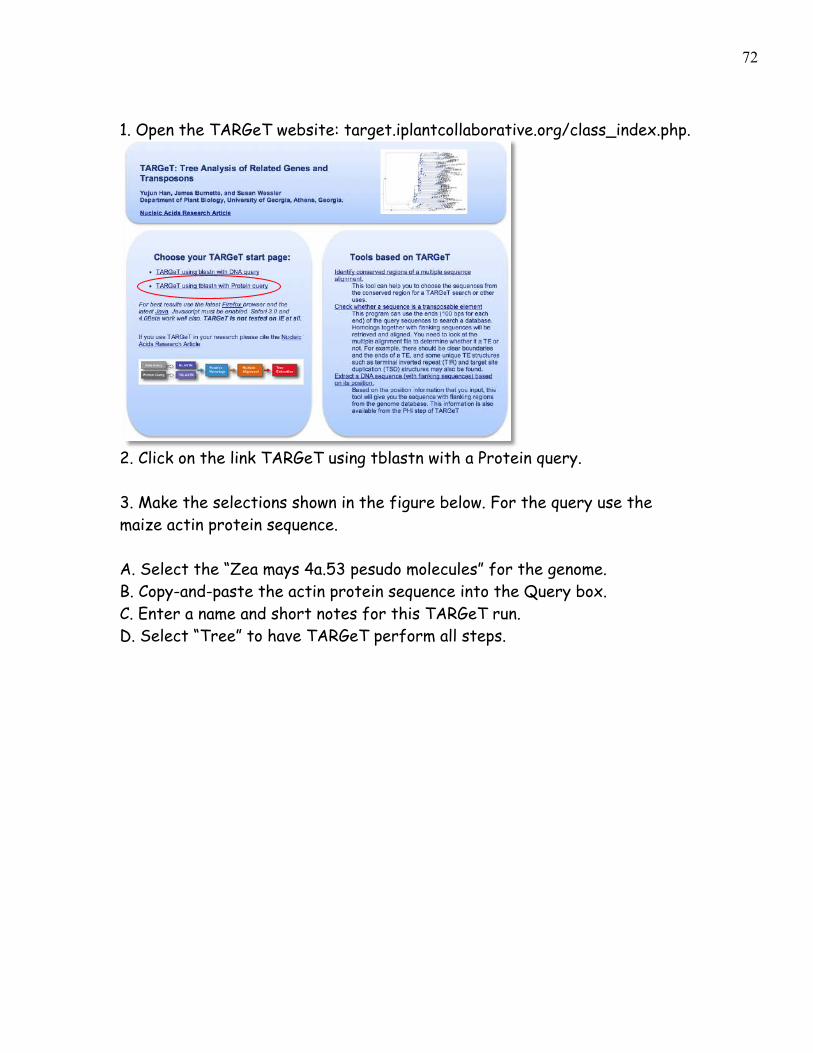
1. Open the TARGeT website: target.iplantcollaborative.org/class_index.php.
2. Click on the link TARGeT using tblastn with a Protein query. 3. Make the selections shown in the figure below. For the query use the maize actin protein sequence. A. Select the “Zea mays 4a.53 pesudo molecules” for the genome. B. Copy-and-paste the actin protein sequence into the Query box. C. Enter a name and short notes for this TARGeT run. D. Select “Tree” to have TARGeT perform all steps.

73
4. The results of a TARGeT search are presented in a single web page. There are 5 tabs of each part of the search. We will go through each tab in class. A. Blast results. To see the standard BLAST output click on the link below the image. The image is a different graphical way to visualize the BLAST results. The Query is shown along the x-axis and the number a quality of the hit to each position of the query is shown in gray scale bars. The darker the color the stronger the match where solid black would be only identities were found at that position whereas grays indicate that similarities and mismatches were found as well.
A.
B.
C.
D.

74
B. PHI Results. PHI is the part of TARGeT that identifies homologs from the blast result. Each sequence that meets the cutoff criteria is considered a homolog. A graphic is produced that shows the gene structure identified by PHI and the homology of the homolog to the query in the coding regions. Again the gray-scale color indicates the degree of homology. In addition a blue ball is used if there is a frame shift and a red ball is used if there is a non-sense codon. The match to actin 1 on chromosome 8 is labeled Zm_pseudo_TARGeT_2. In the image you will see only 4 exons. Remember that actin 1 on chromosome 8 has at least 5 exons, but one of them is non-coding. TARGeT cannot identify non-coding exons when using the results of a tblastn result.
75
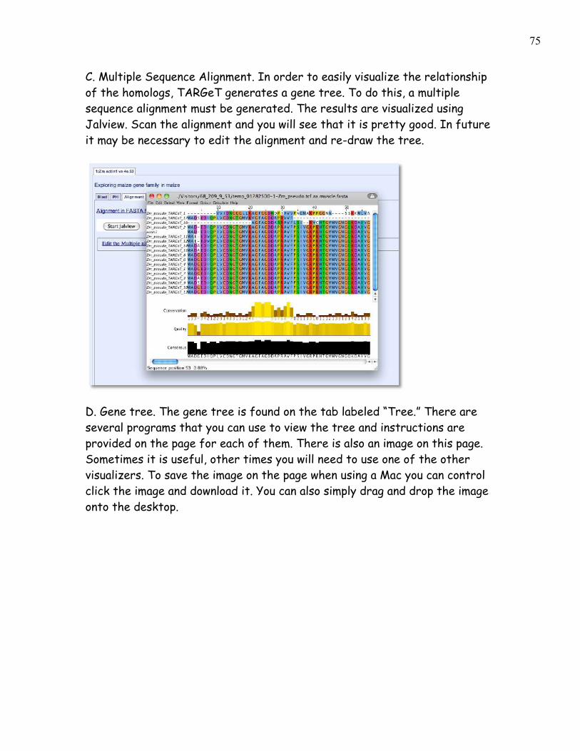
C. Multiple Sequence Alignment. In order to easily visualize the relationship of the homologs, TARGeT generates a gene tree. To do this, a multiple sequence alignment must be generated. The results are visualized using Jalview. Scan the alignment and you will see that it is pretty good. In future it may be necessary to edit the alignment and re-draw the tree.
D. Gene tree. The gene tree is found on the tab labeled “Tree.” There are several programs that you can use to view the tree and instructions are provided on the page for each of them. There is also an image on this page. Sometimes it is useful, other times you will need to use one of the other visualizers. To save the image on the page when using a Mac you can control click the image and download it. You can also simply drag and drop the image onto the desktop.

76
We will discuss the results and how to interpret the tree in class. Finding Actin gene families in other species. Do a TARGeT search with maize actin, but search the rice genome. Do a second search but combine the maize and rice into one TARGeT search. Can you find actin homologs in the human genome using the maize sequence? What would be better the protein sequence or DNA sequence? Why?

77
Appendix: What are phylogenetic trees? Here we have a graphical representation of a phylogenetic tree. Notice the terms and what they refer to.
Before you can interpret a tree you need to understand some terminology. The tips of a tree represent the sampled individuals. These units are called taxa (taxon = singular). We use the term taxa to refer to any level of organization or any named group of organisms. A taxon can represent all individuals in a defined species, a single individual, or a specific amino acid or nucleotide sequence. In a species tree these represent the living organisms that were sampled to reconstruct the phylogeny. In figure 1 our species are labeled taxa A-R. Other types of trees can be made using specific genes or gene families, or in our case these input taxa represent the DNA sequences
Figure 1: This figure shows a graphical representation of a phylogeny. The important features of the phylogenetic tree are labeled.

78
that are obtained from a database. The individual members of the tree are placed on horizontal lines called branches and branches intersect to form nodes. A node represents the common ancestor (in this case the last common sequence) shared by all members that branch from that node. In figure 6 the nodes are labeled with orange dots. Ancestral node sequences are inferred based on the extant (existing) sequences. These nodes represent what the last common ancestor of that group ‘looked like’ to the best of our knowledge. We can infer the sequence of the nodes using the information we have from the tips. The ancestral sequence is a best guess based on the available data. When looking at a tree we are able to visualize the relatedness of the individual members that make it up. Individuals that are placed next to each other on the tree (they are connected by only one node) are called sister taxa. In our case the sister taxa on our transposon trees represent the sequences with the highest level of sequence identity (they are most similar to each other). All members that arise from the same node are said to be in a clade (also called lineages). If all members of a group occur in the same clade the group is said to be monophyletic. If all members of a defined group are not included in a single clade the group is considered either polyphyletic or paraphyletic. Figure 2 shows us the distinction between these two states. In the polyphyletic situation all members of the group do not share a most recent common ancestor. In the paraphyletic case some but not all of the descendants from a most common recent ancestor are included in the group.

79
Figure 2: Monophyletic groups are highlighted in yellow, paraphyletic groups are highlighted in blue, and polyphyletic groups are highlighted in red. The tree of the vertebrates gives us an example of a monophyletic group, the sauropsids, a paraphyletic group, the reptiles, and a polyphyletic group, the warm-blooded animals. In some trees the actual length of the branches connecting the sequences (or species) represent the number of base pair changes over time. So, long branches represent many changes while short branches represent few changes. Branches where more then one tip emerges from one node are called polytomies. If we find polytomies in our transposable element trees, we can assume that the elements placed in the polytomy were very recently active, as all of the sequences are virtually (or are exactly) identical. This example is presented below in Figure 3. In the case of the Ponga, Pongb, Pongc, Pongd, and Ponge clade the branches were too short to draw because these are virtually identical copies in the rice genome, and thus they are represented as a polytomy. We can use this information to design new experiments. Do you find similar clades in the actin gene tree?

80
How are phylogenetic trees constructed? Generally, trees are constructed by identifying shared derived characters, also known as synapomorphies. These characters can be, morphological (e.g., beak dimensions or the presence of a hinged jaw), developmental (e.g., presence of a developmental stage such as gastrulation), or DNA or amino acid sequences. In our case we will use the transposase amino acid sequence as the basis for our comparisons.
Figure 3. A magnified view of Fig 5 that includes the elements most closely related to the Ping element in the rice genome.
Figure 4: Sequence alignments show the relationships between the mammals. The nucleotide sequences alignment visually demonstrates nucleotide similarities and differences while also showing the presence of gaps in the sequences. The level of similarity between the sequences is used to reconstruct the phylogeny.

81
When reconstructing a phylogeny we first collect our data and assign similarity between the individuals based on how many characters differ between them. In our example we would place the specific sequence for each individual into a table, with each individuals sequence in a separate row. The nucleotides (or amino acids) in these rows are then aligned with one another such that each position in the alignment is counted as a character. Any deletions, insertions or base pair differences between the individual’s sequences are highlighted by the alignment. See Figure 4 above for an example of this process. Once the alignments are complete, all pair wise comparisons of the sequences are made. What this means is that each sequence is used as a starting point and is compared to all other sequences present in the alignment. The differences between the sequences (point mutations, deletions and insertions) are noted and the cumulative numbers of changes between sequences are used to generate a value describing how similar the sequences are to one another. From these comparisons a distance matrix is constructed. The more similar a sequence is to another sequence the lower the distance. A sequence compared to itself would have a distance of 0, as all the characters (nucleotides or amino acids) are the same. The more differences we see between any particular comparisons, the higher the distance value. Once the distance matrix is generated based on all of the pair wise comparisons a tree can be drawn. Although this sounds simple, it is not. If we look at 2 taxa there is 1 possible tree, 3 taxa there are 3 possible trees, 4 taxa there are 15 possible trees, 5 taxa there are 105 possible trees. Once we get up to even the modest number of 10 taxa there are 34,459,425 possible trees. If we want to look at 20 taxa there are 8,200,794,532,637,891,559,375 (8x10²⁰) possible trees. Even with the best computers available we cannot efficiently investigate and evaluate the likelihood of all possible trees for any reasonable data set (more then 15 individuals/sequences in the study). Our distance matrix from our multiple alignments can rule out many of these possible trees as impossible given the data, but there are still many trees that ‘fit’ the data. In order to pick the best tree, programs use complex algorithms to find the tree(s) that require the fewest number of changes to explain each step in the tree. A tree with the least number of steps or changes needed to explain the relationships between the taxa is the most parsimonious tree.

82
Parsimony simply defined means ‘less is better’. In other words the path that requires the fewest changes is the most likely answer. There are many different approaches to generate the best tree. The most common methods include: neighbor-joining, Bayesian, and maximum likelihood methods. If you are interested, we can go into more detail about the specifics of these methods. Trees can be rooted or un-rooted. In a rooted tree we have chosen one of the taxa (e.g. one sequence) to be the most ancestral. In a species tree you would use a moderately distantly related species as an outgroup to root the tree. For instance if you wanted to resolve the relationships between the cereals (maize, rice, sorghum, millet, rye, oats etc. ) you may chose another monocot that is not in the same group, such as a lily as your outgroup. You would not want to choose Arabidopsis thaliana, the mustard weed, as the outgroup because it is TOO distant. A. thaliana belongs to the other major class of flowering plants, the dicots, making it too distant to be a reliable outgroup. Outgroups are used to define what is ancestral to all taxa under consideration. The outgroup acts as an anchor, giving the tree an evolutionary framework and orienting the tree. When looking at a tree you will notice that there are numbers on the branches, these represent what we call bootstrap values. This is a confidence level indicator of how probable that clade is based on the data available. If a clade has a bootstrap value of 100 we can be very confident that this relationship is accurately pictured in the tree. If the bootstrap value is 60 we have less confidence in this portion of the tree. The bootstrap value is analogous to a p-value or confidence interval in statistics. Bootstrap values are generated as follows. Let’s say that we have 100 individuals in our data set. We first use all the samples to generate the best fit tree. Once we have the best fit tree we take a sub-set of the original data set, 50 individuals, and re-run the program generating a new tree. The new tree generated from the smaller sub-sample is compared to the original tree generated from all the data. The original tree is evaluated by counting the number of times the same groupings are generated in the sub-sampled data sets. If the same relationships are seen again and again then we have more confidence in their biological reality. A value of 100 indicates that the clade was generated every time the data was sampled. A value of 60

83
indicates that that particular clade was found 60% of the time that the data was sampled. With a bootstrap value of 60, we say that this clade would not be “well supported”. This process of sub-sampling is done over and over again using a different random set of 50 individuals each time. Typically 100 to 200 bootstrap replicates are used to estimate tree reliability. The more often the same clades are constructed using different subsamples, the higher the bootstrap value, and the more confident we are that the relationships are represented accurately. As you might imagine, generating so many trees is an enormous task that would not be possible without computers.

85
Determining the structure of Actin homologs in rice You now know how to do nucleotide blast searches, use the maize genome browser, and build phylogenetic trees. You will now use all of these skills to explore a new genome, the rice genome, and design an experiment where you verify the predicted structure of an actin homolog. The new tool you will learn in this section is PCR primer design. We will also discuss in detail how you will design your experiment. We will then turn to the study of transposable elements and apply all of these tools. A short introduction to rice Oryza sativa is the staple crop grown in Asia. Rice was domesticated twice independently on each side of the Himalayas from the same species. The domesticated rice grown in India is O. sativa indica and the domesticated version grown in China and Japan is O. sativa japonica. Both varieties have been sequenced but the japonica variety was sequenced to higher quality and is the reference version. All of our work will be with japonica and specifically two cultivars EG4 and Nipponbare (pronounced Nippon-bar-ee). Later in the semester you will see why we focus on these two cultivars of rice. Actin homologs in Rice For this experiment we will take the sequence of the actin 1 gene from maie and use it to find actin homologs in rice. We will use the TARGeT program to predict actin homologs and then design a PCR experiment to determine whether the predictions are correct. To make things a little more interesting we will explore most of the homologs TARGeT predicts. You need to keep a detailed record of your computer work. This should be a new Google doc and will eventually be apart of Homework II. 1. Do a TARGeT search for rice actin homologs. Use the japonica rice sequence that is available on TARGeT and change one parameter. What query sequence will you use? What type of blast will you use? How did you obtain this sequence?

86
Click on the “Modify PHI Parameters” and change the “Length of flanking sequence” to 1. (This is a work around to a bug in PHI.)
2. Here is a sample tree obtained from a TARGeT search of the japonica genomic sequence.

87
Which rice actin homolog is most similar to maize actin1? Compare the amino acid sequences of the 10 predicted homologs. How do they compare?
Sometimes it is useful to widen a TARGeT search by relaxing the parameters. The defaults parameters are very stringent and are designed to find very closely related genes. Repeat the TARGeT search but change the following parameters: one for the blast search and three for the PHI search. You can access the parameters by clicking the link “Modify Blast Parameters” and “Modify PHI Parameters.” Make the changes indicated by the red arrows.

88
These changes result in three possible homologs as seen from the tree below.
Two of the homologs look like they may be real genes but more divergent from maize actin than the original ten. One of the new homologs has a stop codon in the first exon. Is this real or a sequencing mistake?
You need to choose one of the putative homologs to study further. We will design primers to amplify all or part of the gene and cDNA from the seedlings you germinated.

89
2. Design Experiment You will need to design your experiment and decide where you are going to design primers. The remainder of this chapter will provide you with information on how to obtain all of the information you will need to design your experiment. The DNA sequence of your homolog can be found on the PHI tab by clicking “Click to view the homologs with flanking sequence.” Note whether the gene is on the top (+) or bottom (-) strand. TARGeT reports the DNA sequence in top (+) strand only. If your gene is on the bottom strand you will need to reverse and complement the sequence. Remove the first nucleotide and the last nucleotide from this sequence. (This is a work around to a bug in PHI.) There is the option to reverse and complement the sequence on the FASTA format page of TARGeT. The amino acid sequence of your homolog can be found on the PHI tab by clicking “Click to view the PHI results.” The start and stop positions of the exons can be found by clicking the “Click to view exon positions” link. The exon positions are given based on the top strand and with respect to the contig. You will need to translate the numbers to the sequence you have. If your sequence is on the top strand the first exon starts at position 1. So if the first exon is from nt 23197603 to 23197992 on the contig it is 1 to 390 on the sequence obtained from PHI. (23197992 - 23197603 +1 = 390.) Draw a diagram to keep track of these numbers. If your gene is on the bottom strand exon starts at the highest number. If you reverse and complemented your sequence earlier then you will need to set the highest number as 1 and then subtract the subsequent numbers from the highest number. So if the first exon goes from 3233059 to 3233000
1023 1157 390 1 3137 3238

90
the 3233059 is nt 1 of exon 1. The end of exon 1 is 3233059-3233000 + 1 = 60. Continue this with the other exon positions. Primer Design PCR primers are easily designed by using a program called Primer3Plus: http://www.bioinformatics.nl/cgi-bin/primer3plus/primer3plus.cgi. There are many parameters and much folklore about designing primers. These instructions require you to modify the minimal number of parameters to design quality primers. Typically primers are designed in pairs. A good pair of primers will meet these criteria:
1. Each primer should be 18-25 base pairs long. 2. The 3’ nucleotide of the primer should be a G or C. This is called the G/C clamp. 3. The G/C content should be around 50%. 4. The melting temperature (Tm) of each primer should be close to 60˚C. The difference between the Tms of a primer pair should 5˚C or less. 5. Neither primer should form a hairpin. 6. Primers should not be self-complementary. 7. Partners should not complement. 8. All primer sequences are reported in 5’ to 3’ direction. 9. The product size should be between 200 and 2000 nt for Taq DNA Polymerase.
Before you open Primer3Plus you will need to plan the region you want the primers to bind and the maximum length of the PCR product. Target Region Where do you want to put the primers? In exons? Introns? Which exon or introns? Once you decide this you need to determine the sequence position between the primer regions. This region is called the “Target” in Primer3Plus. This is given as the start position and the length. For example the example above if you wanted primers in exon 1 and exon 3 you would determine that the start of the Target is 390 and the length of the Target is 3137 – 390 or 2747.

91
Maximum PCR product length Based on the region that you want the primers you can determine the maximum length of the PCR product. In this case we want the primers in exon 1 and exon 3 so the maximum PCR product is 3238 – 1 +1 or 3238 bp. Would this be a good PCR product length? After you have this information you can design primers. 1. Open the Primer3Plus website: http://www.bioinformatics.nl/cgi-bin/primer3plus/primer3plus.cgi.
1. Copy the genomic sequence into the large textbox. 2. In “Targets” enter the limits of the Target region you determined
above.
2. Click on the “General Settings” Tab.
1
2

92
3. In the field for “Product Size Ranges” delete all of the ranges. Enter a lower value of 200 bp and the highest value will be the maximum length of the PCR product you determined above. In this case we could enter 200-3300. Primer3Plus will make the smallest sized product possible.

93
4. Click on the “Advanced Settings” Tab. Set the GC Clamp to 2. This will require that the last two 3’ nucleotides be a G or C.
5. Click the green “Pick Primers” button. 6. Results come back quickly. The ‘best’ primer pair is listed at the top. Other good pairs are listed further down the page. The first pair is good and would be the ones ordered. The “Left” or “Forward” primer is highlighted in purple and the “Right” or “Reverse” primer is highlighted in yellow. 7. Rename the primers to a meaningful name keeping the “_F” or “_R”.

94
8. Save this page or take a screen shot. On a Mac you can create a PDF by selecting File->Print. In the Print dialog box select save as PDF. Select a location save the file.
Primer 3 rarely fails to find good pairs. However, if Primer3 cannot find primers you can use the statistics table on the results page to modify and repeat the search. The statistics tell you how many primers were considered and why they were rejected. This information can be used to modify the parameters of Primer 3.

95
9. To order the primers, go to the course Data webpage. There you will notice a short form to fill out. Primers will be ordered from IDT. They will be synthesized and should arrive the morning of the day of class we will use them. Experimental Protocols. The DNA extraction will be the same protocol found on pages 24-25. The PCR protocol can be found in your notebook.

96
RNA Extraction Extracting RNA is similar to extracting DNA except that RNA is very unstable. Also, we are not concerned with RNA contamination in a DNA sample, but DNA contamination in an RNA sample is bad. RNA is unstable at temperatures above room temperature due to 2’ OH group on the ribose. The 2’ OH will attack the 3’ Phosphate backbone and result in breaking the RNA backbone. RNA is also unstable due to the abundance to RNase enzymes that are everywhere. For RNA work we use RNase Free tips, tubes, and reagents. Even autoclaved, double distilled, filtered water is not considered RNase Free. The kits we use contain RNase blockers. For RNA extraction the reagents contain guanidine salt, which denatures proteins. Guanidine salts are very irritating so do not get these in your eyes. The reverse transcription kit contains a protein called RNasin that a very effective inhibitor of RNases. RNase A and RNase H are the two RNases that you need to know about. RNaseA is very abundant, highly stable in all conditions (included surviving autoclaving). It is an endonuclease that cleaves between C and U residues. The second RNase is RNaseH. This enzyme is actually a subunit of reverse transcriptase and degrades the RNA partner of a RNA-DNA hybrid. You will purposefully add RNaseH at the end of the reverse transcripase reaction. You need to be very careful and work quickly when working with RNA. You must wear gloves to protect your samples from RNases on your hands. You will use tips, reagents, and water that are RNase free. RNA samples must be kept on ice and are stored at -80˚C. RNA Extraction 1. Use about 100 mg of tissue. One embryo is enough. 2. Place the tissue in a mortar and grind with Liquid Nitrogen. Before the nitrogen completely evaporates pour into a 1.5 ml tube. Add more Nitrogen if necessary. Do not close the cap. Not all of the tissue will transfer.

97
3. Add 450 µl RLT. Vortex. (Repeat 1 and 2 for next sample. Continue when all samples are at this stage.) 4. Pipette lysate onto a QiAshredder spin column (lilac colored column). Spin 2 minutes at full speed. This will be very viscous. 5. Transfer flow through to a new 1.5 µl tube. Do not disturb the pellet. Throw away the lilac colored column. 6. Add 225 µl Ethanol. 7. Pipette sample to RNeasy column (pink). Spin 30 secs at high speed. 8. Add 350 µl RW1 to the column. Spin. Discard the flow through. 9. Add 80 µl of DNase solution to the column. 10. Incubate at RT for 15 min. 11. Add 350 µl RW1 to the spin column. Spin. 12. Add 500 µl RPE to column. Spin 30 sec. 13. Empty collection tube. Add 500 µl RPE to column. Spin 2 min. 14. Place Column into a new collection tube. Spin 1 min at full speed. 15. Place Column into the RNase free 1.5 ml tube. Place 30 µl RNase free water on column. Spin 1 min. Keep the RNA on ice from now on. Check the RNA quality. 1. Place 5 µl of RNA into a new tube. Add 10 µl of water and 2 µl of loading dye. Load a 1.5% gel. Include a DNA ladder. Reverse Transcription using the Promega ImpromtII Kit 1. Mix Oligo dT primer with RNA

98
RNA 2 µl oligodT 1 µl H2O 2 µl 5 µl Heat 70˚C for 5 minutes. Chill on ICE for at least 5 minutes. 2. Centrifuge. 3. Add 15 µl of Reaction mix to each RNA + primer sample. Mix by carefully pipetting up and down. 4. Put in thermocycler for: Anneal 25˚C 5 min. Extend 42˚C 60 min. Inactivate 70˚C 15 min. 5. Add 0.5 µl RNase H. Incubate for 20 min at 37˚C. cDNA should be stored at -20˚C freezer temperature. 6. Use 1.0 µl of cDNA to a 25 µl PCR reaction.

99
Dawkins: The Greatest Show on Earth Assignments for in-‐class discussions Thurs, Feb 11 (through p 42) Chapter 1: Only a Theory? Chapter 2: Dogs, Cows and Cabbages Thurs, Feb 18 (through p 82) Chapter 3: Macroevolution Tues, Mar 2 (through p 141) Chapter 4: Silence and Slow time (clocks) Chapter 5: Before our Very Eyes Tues, Mar 16 (through p 207) Chapter 6: Missing Link? What do you Mean Missing? Chapter 7: Missing Persons? Missing No Longer. Tues, Mar 23 (through p 284) Chapter 8: You Did it Yourself in Nine Months Chapter 9: The Ark of the Continents Thurs, March 25 (to the end) Chapter 10: The Tree of Cousinship Chapter 11: History Written All Over Us Chapter 12: Arms Race and Evolutionary Theodicy Chapter 13: There is Grandeur in this View of Life

100

99
Chapter 2: Transposable Element Background
2.1. The Discovery of Transposable Elements
It all began more than 60 years ago with a far-sighted scientist named Barbara McClintock who was studying the kernels of what we informally call “Indian corn.” You know what it looks like—those ears with richly colored kernels that we associate with Thanksgiving and that we call maize. Maize and corn are the same species. Maize is a grass that is taxonomically related to other familiar cereal grasses like barley, rice, wheat and sorghum. By the 1920s, researchers had found that maize kernels were ideal for genetic analysis because heritable traits such as kernel color and shape are so easy to visualize. The results of early studies on maize led to an understanding of chromosome behavior during meiosis and mitosis. As a result, by McClintock’s time, maize was one of two model genetic organisms - the other being Drosophila melanogaster (the fruit fly). As early as the 1920’s it was known that maize had 10 chromosomes [this is the haploid number (n) - maize, is a diploid (2n) with 2 sets of 10 chromosomes]. In addition to being a superb geneticist, McClintock was one of the best cytologists in the world and her specialty was looking at whole chromosomes. Maize was idea for this analysis because it has a large genome (recall - 2500 Mb) and its chromosomes were easily visualized using a light microscope. The first thing of note that McClintock did as a scientist was to distinguish each of the 10 maize chromosomes of maize. This was the first time anyone was able to demonstrate that the chromosomes (of any organism) were distinct and recognizable as individuals.

100
In the course of her studies of various maize strains, she noticed the phenotype shown below in Figure 1a. This phenotype is characteristic of chromosome breakage. While chromosome breakage is commonly observed in maize, it had not previously been observed at a single site (locus) in one chromosome. In one particular strain chromosome 9 broke frequently and at one specific place or locus. After considerable study, she found that the breakage was caused by the presence in the genome of two genetic factors. One she called Ds (for Dissociation -it caused the chromosome to “dissociate”), and it was located at the site of the break. But another genetic factor was needed to activate the breakage. McClintock called this one Ac (for Activator). Because she could not genetically map the position of Ac in the genome she hypothesized that it was capable of moving around (transposing). For example, Ac could move from chromosome 1 to chromosome 3. As she followed the descendents of this strain, she identified rare kernels with but fascinating phenotypes. One such phenotype was a colorless kernel containing pigmented spots. This is summarized in Figure 1b.
Figure 1. New phenotypes in corn are produced through the movement of the Ds transposable element on chromosome 9. (a) A chromosome fragment is lost through breakage at the Ds locus. Recessive alleles on the homologous chromosome are expressed, producing the colorless sector in the kernel. (b) Insertion of Ds in the C gene (top) creates colorless corn kernel cells. Excision of Ds from the C gene through the action of Ac in cells and their mitotic descendants allows color to be expressed again, producing the spotted phenotype.
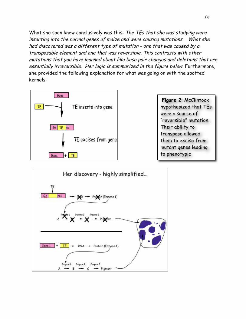
101
What she soon knew conclusively was this: The TEs that she was studying were inserting into the normal genes of maize and were causing mutations. What she had discovered was a different type of mutation - one that was caused by a transposable element and one that was reversible. This contrasts with other mutations that you have learned about like base pair changes and deletions that are essentially irreversible. Her logic is summarized in the figure below. Furthermore, she provided the following explanation for what was going on with the spotted kernels:
Figure 2: McClintock hypothesized that TEs were a source of “reversible” mutation. Their ability to transpose allowed them to excise from mutant genes leading to phenotypic reversion.

102
2.2 What DNA transposable elements look like to the geneticist (Ac, Ds) As you have seen Barbara McClintock discovered the TEs Ac and Ds when she figured out that they were responsible for the spotted kernel phenotypes. She was a geneticist - and their main experimental tool is the genetic cross. Here are some of the properties of Ac/Ds that McClintock figured out through observation of kernel phenotypes and by performing carefully designed crosses: (1) Ac and Ds could insert into a variety of genes - e.g. those involved in pigment production, starch biosynthesis, and early embryo development, to name but a few. (2) Ac and Ds were normal residents of the corn genome - they were not, for example, introduced into the genome by a virus. (3) Ds could not move without Ac in the genome, whereas Ac could move itself or Ds. Thus, Ac was called an autonomous element while Ds was called a non-autonomous element.
TEs are in all organisms: After her initial results were reported in the late 1940’s, the scientific community thought that TEs were oddities and possibly restricted to maize and perhaps to a few other domesticated plant species. However, this proved not to be the case as in subsequent years TEs were discovered in the genomes of virtually all organisms from bacteria to plants to human. It is for this reason that McClintock was awarded the Nobel Prize in Medicine or Physiology in 1983, almost 40 years after her discovery. We will return to Barbara McClintock often during this course.
Figure 3 Summary of the main effects of transposable elements in corn. Ac and Ds are used as examples, acting on the C gene controlling pigment. In maize (but not many other organisms), normal alleles are capitalized and mutant alleles are written in lower case. In addition, McClintock designated alleles caused by the insertion of a TE as “mutable”, m for short [e.g. c-m(Ds) or c-m(Ac)].

103
2.3 What transposable elements look like to the molecular biologist (Ac,Ds): With the advent of molecular cloning biologists were able to isolate and sequence gene-sized fragments of DNA from the genomes of plants and animals. They say that a picture is worth a thousand words. So… here is a simplified figure showing what Ac and Ds look like at the DNA level.
Ac contains a single gene - that encodes the transposase. Figure 4 shows how this protein catalyzes the movement of Ac and Ds.
Figure 4: Molecular structure of Ac and Ds. Ac: Tpase is the gene encoding the transposase enzyme which is necessary for movement of both Ac and Ds. Ds: Ds requires Ac for movement because it is a defective version of Ac where the Tpase gene has been deleted. Yellow arrows at the ends are the terminal inverted repeats - this site where transposase binds and cuts the element out of the surrounding genomic DNA.
Figure 5 Activator transposase catalyzes excision and integration. The maize Ac element encodes a transposase that binds its own ends or those of a Ds element, excising the element, cleaving the target site, and allowing the element to insert elsewhere in the genome.

104
Like many other proteins, the transposase protein can multi-task. First, it is a DNA binding protein that is able to bind specifically to the ends of the Ac element. The protein also binds to the ends of Ds as it is identical to the Ac ends. Such “sequence-specific binding” is mediated by precise contacts between the amino acids of part of the transposase (called the binding domain) and the precise nucleotide sequences at the Ac (and Ds) ends. Second, it is an enzyme. Once bound, the two transposase molecules form a dimer (via protein-protein interactions) and another region of the transposase (called the catalytic domain) cuts the element out of the surrounding genomic DNA. The two transposase proteins bound to the TE then cuts the chromosome at another site (the target) in the host genome and the TE inserts. Finally, for now at least, there is one other feature of TEs that needs to be introduced. This is the target site duplication (TSD) that is created during insertion of virtually all TEs. How it is generated is shown below in Figure 6.
Figure 6: An inserted element is flanked by a short repeat. A short sequence of DNA is duplicated at the transposon insertion site. The recipient DNA is cleaved at staggered sites (a 5-bp staggered cut is shown), leading to the production of two copies of the five-base-pair sequence flanking the inserted element. This is called a target site duplication (TSD).

105
2.4. What transposable elements look like to the bioinformaticist As you know, Human Genome Project ushered in the genomics era which is characterized by the availability of increasing amounts of genomic sequence from a variety of plant and animal species [animals - including human, fruit fly (Drosophila), earthworm, dog, mouse, rat, chimp; plants - including Arabidopsis thaliana, rice, maize (corn) cottonwood (a tree)]. For now, it is sufficient to know that TEs make up the vast majority of the DNA sequence databases and recognizing TEs in genomic sequence is usually the first step in the modern analysis of TEs. The elements you will be analyzing in experiment 2 are the Ping and mPing (for miniature Ping) elements - which were first identified by computational analysis of the rice genomic sequence (see page 14 below for how this was done). The figure below shows that Ping is the larger coding element like Ac. Unlike Ac Ping contains 2 genes (ORF1 + Tpase).
As you can see, like Ds which is derived from Ac by a large deletion, mPing is derived from Ping by a large deletion. Our hypothesis is that Ping encodes a protein that binds to the ends of mPing and catalyzes its transposition. So, this should be a snap, right? Let’s just study an mPing element that is inserted into a rice gene and monitor its movement in the same way as McClintock did with spotted kernels (rice grains in this case). Well, unfortunately, we can’t do that - because - like most TEs in the genome, mPing is not inserted into a rice gene - but rather - it is inserted between rice genes!
Figure 7: Ping encodes two genes: the transpoase (TPase) and ORF1 (open reading frame) (function unknown at this time). The red arrows are the terminal inverted repeats (14bp). mPing is 253bp + 177bp long.

106
2.5. Digression - how can organisms survive with so many TEs? Where are TEs located in the genome? At this point we need to go up to 30,000 feet in order to understand a larger concept: the connections between TEs, evolution and natural selection. In short, the distribution of TEs in most genomes is due to the action of natural selection —the foundation for all modern biology. Most of you probably understand these concepts already. Just in case, here is a brief review… There are three kinds of selection that will need to understand: *Negative selection *Neutral selection *Positive selection It is important first to know something about natural selection itself. Here’s a slightly edited version of its definition in Wikipedia: “. . . In the context of evolution, certain traits or alleles of a species may be subject to selection. Under selection, individuals with advantageous or `adaptive’ traits tend to be more successful than their peers reproductively—meaning they contribute more offspring to the succeeding generation than others do. When these traits have a genetic basis, selection can increase the prevalence of those traits, because offspring will inherit those traits from their parents.” Negative selection is the elimination of a deleterious trait from the population by natural selection. It is also called “purifying selection.” In the context of TEs, insertions into genes are deleterious and, as such, are eliminated from the population. The word elimination in this case means that an individual with the TE insertion will either not be viable or will not be able to reproduce. Neutral selection describes changes in the gene pool of a species that are a result of accumulated random neutral changes that do not convey any particular advantage to a species. Accordingly, neutral selection does not depend upon adaptation, fitness, and natural selection. Positive selection occurs when a certain allele has a greater fitness than others, resulting in an increase in frequency of that allele. This process can continue until the entire population shares the fitter phenotype, then the allele is said to be

107
“fixed” in the population. An example of this is a TE insertion that affects a gene in some positive way that makes the organism more adaptive in a particular environment. Such a change would be incredibly rare, though, because there are thousands of genes in a genome where a TE can insert and most insertions in a gene are harmful. Think of a population where the climate has changed and become much drier. Increasing the expression of one particular gene in the genome might increase drought tolerance and allow an organism with such a “mutation” to survive. For a TE to insert into just that gene, in the right place so that it increases the expression of the gene, is extremely unlikely. However, when we think of probabilities it is important to keep in mind that there are lots of TEs in a genome, that there can be many individuals in a population and finally - evolution occurs over very long time periods - that’s why it’s called evolution, not revolution! This concept will be described in greater detail in “The Making of the Fittest”. So what does all this have to do with transposable elements? Transposable elements can insert into all regions of the genome - in genes and between genes. However, if we look at an entire genome, we usually find most of the TEs between genes and in noncoding regions of a gene (e.g like introns). This is because insertions into genes have fallen victim to negative selection. In contrast TEs between genes remain for generations, hundreds of generations, because they are not harmful. Rather, they are usually neutral and may even be beneficial. Most of the TEs in the genome are INACTIVE This leads to a second point you need to remember: The vast majority of transposable elements in a genome are inactive (they can’t move anymore). TEs can be inactivated in one of at least two ways—through mutation or through what is called “epigenetic silencing.” The mutation part is easier to understand. All DNA is susceptible to mutation - usually base pair changes or deletions. This happens (very rarely) when there is an error during replication and the wrong base is inserted - for example a G is put opposite T (instead of an A). This change could alter an amino acid in a protein. Mutation can also happen by “free radicals” - chemicals that accumulate in our cells and can damage our DNA. Finally, mutagens in our environment - like UV light or cigarette smoke - can damage our DNA.

108
There are dramatically different consequences of a mutation in a gene vs. in a TE. Stately simply, mutation in a gene is usually eliminated from the population by natural selection (negative selection), whereas mutation in a TE will be neutral and, as such, will persist in the population. Thus, unlike genes, TEs will accumulate mutations and become inactive. (NOTE - TES AND GENES SUSTAIN MUTATIONS AT THE SAME FREQUENCY. HOWEVER, IF YOU STUDY AN ORGANISMS GENOME, MOST OF THE GENES WILL BE ACTIVE WHILE MOST OF THE TEs WILL HAVE SUSTAINED INACTIVATING MUTATIONS) Epigenetic regulation of TEs (to be discussed later in the course in grueling detail). For now, suffice it to say that eukaryotic chromosomes exist in the nucleus as chromatin - an equal mixture of DNA and protein. The basic unit of chromatin is the nucleosome - about 180bp of DNA wound around a core of histone protein (shown as a ball in figure 8 below). Chromatin can be loosely organized (open chromatin, called euchromatin) or highly condensed (where nucleosomes are tightly packed, called heterochromatin). You can see both of these chromatin types in Figure 8. In most plant genomes such as maize, transposable elements are frequently clustered and associated with condensed chromatin. Genes in condensed chromatin cannot be expressed and are inactive. This is the fate of the vast majority of the TEs in a genome.
So let’s say it again: Most TEs in the genome of plants and animals are rendered inactive by mutation or by epigenetic silencing.
Figure 8. The nucleosome in decondensed and condensed chromatin. (b) Chromatin structure varies along the length of a chromosome. The least-condensed chromatin (euchromatin) is shown in yellow, regions of intermediate condensation are in orange and blue, and heterochromatin coated with special proteins (purple) is in red.

109
Chapter 3: From a single element to all of the elements in the genome In chapter 2 you were introduced to Ping/mPing. It turns out that the rice genome can contain up to 1000 copies of mPing and from 0 up to seven Ping elements (this depends on the rice strain). Ping and all of the mPing elements in the rice genome make up a TE family. The genomes of plants and animals contain many different families of transposable elements. This concept is central to understanding what genomes are made of. What is a TE family? We have already been introduced to two TE families. One family (from maize) contains the Ac and Ds elements while the second family (from rice) contains Ping and mPing elements. In functional terms, a TE family contains all the elements that can be mobilized by a particular transposase. A TE family usually contains autonomous elements (e.g. Ac, Ping) and nonautonomous elements (e.g. Ds, mPing) elements. When we analyze the DNA sequence of entire genomes we often find that a family contains several elements including one or more autonomous elements and many copies of nonautonomous elements (the maize genome has over 50 copies of Ds and, as mentioned above, some rice genomes have up to 1000 copies of mPing). The transposase encoded by the Ac element can mobilize both Ac and Ds elements. If there is no Ac element in the genome, all of the Ds elements will be “stuck” where they are - they will not able to move elsewhere in the genome because there is no transposase to catalyze their movement. The same is true for Ping and mPing in rice – mPing will be stuck in place if Ping is not in the genome. A very important feature of TE families is that each family is independent. In practical terms this means that the Ac transposase cannot mobilize Ping or mPing elements and, similarly, the Ping transposase cannot mobilize Ac or Ds elements. Or, as shown in Figure 1, the transposase from family A cannot move the elements in family B. The reason for this is simple. A transposase works by first binding to a specific DNA sequence near the ends

110
of the element called the Terminal Inverted Repeat or TIR. The Ac transposase first binds to a specific sequence of nucleotides that is only near the ends of Ac and Ds elements while the Ping transposase binds to a specific sequence that is only near the ends of Ping and mPing elements. (Recall that in addition to catalyzing chemical reactions, proteins can also bind to DNA. Transposases are proteins that do both: bind to DNA and then catalyze the transposition reaction.)
What is a TE superfamily? After Barbara McClintock discovered Ac and Ds (in the 1940’s) she then discovered a second TE family, which she called Spm (for Suppressor-mutator - a long story!). The autonomous element in this family is called Spm and the nonautonomous element is called dSpm (for defective-Spm). Thus, Spm-dSpm is another TE family. McClintock’s discoveries resulted from genetic analyses of corn plants. After the discovery of TEs in maize, researchers working with other model organisms, including Antirrhinum majus (a.k.a. snapdragon) Drosophila melanogaster (a.k.a. the fruit fly) and Caenorhabditis elegans (a.k.a. the worm) also identified TEs through genetic studies. In the 1980’s when it
Figure 1: A TE family contains autonomous elements and all the nonautonomous elements in the genome that its transposase can move. Genomes have many TE families that are independent. This is because the transposase of Family A, for example, cannot bind to the ends of the elements from Family B and vice versa.

111
became possible to isolate specific genes, researchers isolated McClintock’s Ac, Ds, Spm and dSpm elements and the elements from snapdragon (called Tam 1,2,3 etc), the fly (called P-elements, mariner elements and others) and the worm (called Tc1, 2 and 3 elements). When the DNA sequences of these elements were determined and compared (by computer analysis), researchers were surprised to find that the transposases encoded by some of the elements from different species, even from different kingdoms (animal vs. plant), were similar. For example, the amino acid sequence of the transposase from the maize Ac element was similar to the amino acid sequences of the transposases of Tam3 from snapdragon and the P element from the fly, while the transposases of the mariner (fly) and Tc1 (worm) elements were similar. These similar transposases were subsequently organized into superfamilies. Fortunately, after all of the sequencing of genomes and comparisons of TEs, there are now known to be fewer than 10 superfamilies of transposases. Some superfamily names and elements and some members include: hAT (includes Ac, Tam3, P elements), CACTA (includes Spm, Tam1), PIF/Harbinger, Mutator and Mariner. The distribution of some of the superfamilies across the tree of life is summarized in Figure 2.
Figure 2. Distribution of the major groups of DNA transposons across the eukaryotic tree of life. The tree depicts 4 of the 5 “supergroups” of eukaryotes where DNA transposons have been detected. The occurrence of each TE superfamily is denoted by a different symbol. (Feschotte ·Pritham Annu. Rev. Genet. 2007.41:331-68).

112
How many families and superfamilies can an organism have in its genome? In short, many. First, members of most superfamilies are present in all plant genomes including maize, rice and Arabidopsis, and are also present in most animal genomes (Figure 2). For example, the rice genome has Mariner, PIF/Harbinger (Ping), hAT (Ac/Ds), CACTA and Mutator elements. In addition, each superfamily usually contains many families in one genome. Structural features shared by superfamily members: Before you can study a TE superfamily, we need to look closely at the structural features of transposable elements in more detail because these features are usually shared within a superfamily.
The terminal inverted repeat (TIR): In the figure above, the sequence of the blue triangles is shown. Look closely and you will see that the sequence of the right TIR is the reverse-complement of the left TIR. These sequences help define a TE family because they are bound by TPase produced by a family member. While all
Figure 3: Structural features of transposable elements that are shared by superfamily members. TSD = target site duplication, TIR = terminal inverted repeat, Tpase = transposase gene that is present in all autonomous elements, ORF1 – a second gene that is only encoded by members of the Ping/PIF/Harbinger superfamily

113
members of a TE family have identical or near identical TIRs, the TIRs of superfamily members (elements from different species) are usually similar but not identical. In addition, the length of the TIR can vary. For example, the length of the Ping TIR is 15bp while the length of the Ac TIR is 11bp. Target site duplication The target site duplication (TSD) is a direct repeat sequence that flanks the TIR. It is generated during the insertion of virtually all TEs into genomic DNA. How it is formed is shown below.
The length of the TSD, but usually not the sequence, is a common feature of a TE superfamily. For example, members of the hAT superfamily (Ac, Tam etc) all have an 8bp TSD, while members of the Mutator family have a 9bp TSD. Ping has a 3 bp TSD that is almost always TAA or TTA. The Transposase (Tpase) gene: The sequence of the TPase is also characteristic of a superfamily. In fact, the tpase sequence (or part of it) is THE feature used to define
Figure 4: An inserted element is flanked by a short repeat. A short sequence of DNA is duplicated at the transposon insertion site. The recipient DNA is cleaved at staggered sites (a 5-bp staggered cut is shown), leading to the production of two copies of the five-base-pair sequence flanking the inserted element.

114
superfamilies. Later in the course you will use the sequence of the TPase and the sequence of the TIR to find Ping family members in rice and in other plant species. Using computational analysis to find all elements related to Ping in rice and other genomes: You can identify all TEs related to Ping in rice because the whole genome of rice has been sequenced. To do this one performs a Blast search using either the DNA sequence of the whole element or the protein sequence of the TPase. Using the whole element as query would retrieve only very related elements. To explore the diversity of the superfamily (in the rice genome or in other sequenced genomes) you would use the amino acid sequence of the TPase protein or part of the sequence. The Blast results in either case would be numerous and determining relatedness of the elements is impossible from a Blast output. To analyze the relationships between large numbers of related DNA sequences we use phylogenetic trees. These trees are similar to the species trees you have seen in other classes. You have learned about sequence alignments using a single query of a large database. The result is many ‘hits’ that must be compared to each other in order to determine which sequences are most closely related. This process is called multiple alignment and there are several computer programs for this task. Once you have a multiple alignment a different software program is used to construct a phylogenetic tree. The process of generating a tree can be time consuming and tedious. Luckily for us Yujun Han (a graduate student in the Wessler lab) streamlined this process by creating a single web-based bioinformatics pipeline called TARGET. You will learn all about TARGET during class and you will use it often during the rest of the semester. A Brief Look at a Phylogenetic Tree of Ping-like elements in rice Look at the phylogenetic tree of the elements related to Ping in rice in Figure 5. The red arrow is pointing to THE Ping element. This tree was constructed using a part of the TPase amino acid sequence. Shown beside the tree is the DNA structure of each element. We will discuss this tree in class and point out its features and key terms (also later in this section). You will be making lots of your own trees in this class. This is just meant as an introduction and overview.

115
Figure 5: A phylogenetic tree of the relationships between Ping/Pong-like elements in the rice genome. The structure of each element is shown at the right with the transpose gene drawn as a black box, ORF1 drawn as a gray box, and arrows for the terminal inverted repeats (TIRs). Ping is indicated with a red arrow. Zhang et al. (2004) Genetics. 166: 971-986.
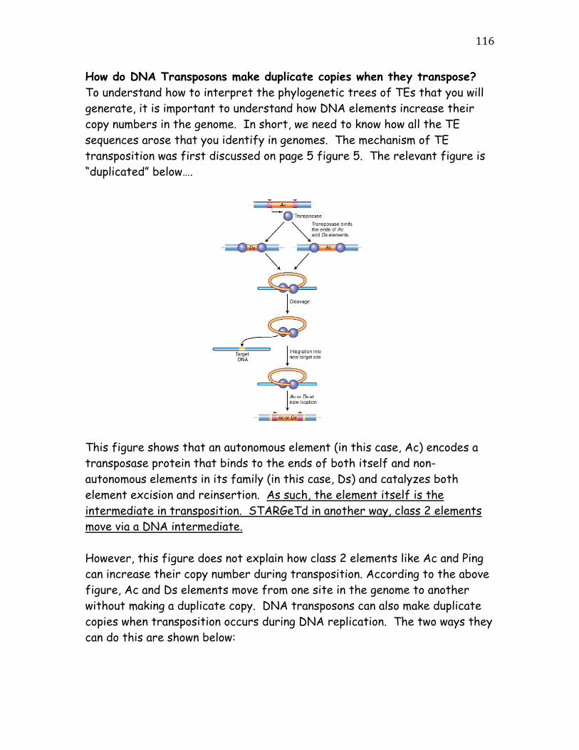
116
How do DNA Transposons make duplicate copies when they transpose? To understand how to interpret the phylogenetic trees of TEs that you will generate, it is important to understand how DNA elements increase their copy numbers in the genome. In short, we need to know how all the TE sequences arose that you identify in genomes. The mechanism of TE transposition was first discussed on page 5 figure 5. The relevant figure is “duplicated” below….
This figure shows that an autonomous element (in this case, Ac) encodes a transposase protein that binds to the ends of both itself and non-autonomous elements in its family (in this case, Ds) and catalyzes both element excision and reinsertion. As such, the element itself is the intermediate in transposition. STARGeTd in another way, class 2 elements move via a DNA intermediate. However, this figure does not explain how class 2 elements like Ac and Ping can increase their copy number during transposition. According to the above figure, Ac and Ds elements move from one site in the genome to another without making a duplicate copy. DNA transposons can also make duplicate copies when transposition occurs during DNA replication. The two ways they can do this are shown below:

117
1. Gap repair using the sister chromatid to repair the excision site….

118
2. Transposition from a replicated site to an unreplicated site, which is then replicated:
What you should note is that no matter which way a class 2 element moves, the element and its duplicate(s) are identical. Over time (evolutionary time that is), the element sequences muTARGeT independently (e.g. by errors introduced during DNA replication). Elements accumulate mutations over time (they diverge). Thus, the extent of sequence divergence between elements is a measure of the time since duplication. In the figure you also see the term – transposon footprint. This will be discussed briefly in the class but in much more detail later as it will be the basis of at least one experiment you will be doing.
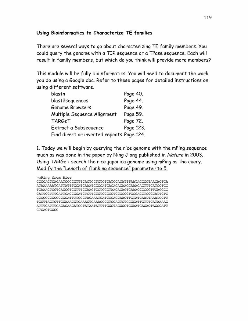
119
Using Bioinformatics to Characterize TE families There are several ways to go about characterizing TE family members. You could query the genome with a TIR sequence or a TPase sequence. Each will result in family members, but which do you think will provide more members? This module will be fully bioinformatics. You will need to document the work you do using a Google doc. Refer to these pages for detailed instructions on using different software.
blastn Page 40. blast2sequences Page 44. Genome Browsers Page 49. Multiple Sequence Alignment Page 59. TARGeT Page 72. Extract a Subsequence Page 123. Find direct or inverted repeats Page 124.
1. Today we will begin by querying the rice genome with the mPing sequence much as was done in the paper by Ning Jiang published in Nature in 2003. Using TARGeT search the rice japonica genome using mPing as the query. Modify the “Length of flanking sequence” parameter to 5. >mPing from Rice GGCCAGTCACAATGGGGGTTTCACTGGTGTGTCATGCACATTTAATAGGGGTAAGACTGA ATAAAAAATGATTATTTGCATGAAATGGGGATGAGAGAGAAGGAAAGAGTTTCATCCTGG TGAAACTCGTCAGCGTCGTTTCCAAGTCCTCGGTAACAGAGTGAAACCCCCGTTGAGGCC GATTCGTTTCATTCACCGGATCTCTTGCGTCCGCCTCCGCCGTGCGACCTCCGCATTCTC CCGCGCCGCGCCGGATTTTGGGTACAAATGATCCCAGCAACTTGTATCAATTAAATGCTT TGCTTAGTCTTGGAAACGTCAAAGTGAAACCCCTCCACTGTGGGGATTGTTTCATAAAAG ATTTCATTTGAGAGAAGATGGTATAATATTTTGGGTAGCCGTGCAATGACACTAGCCATT GTGACTGGCC
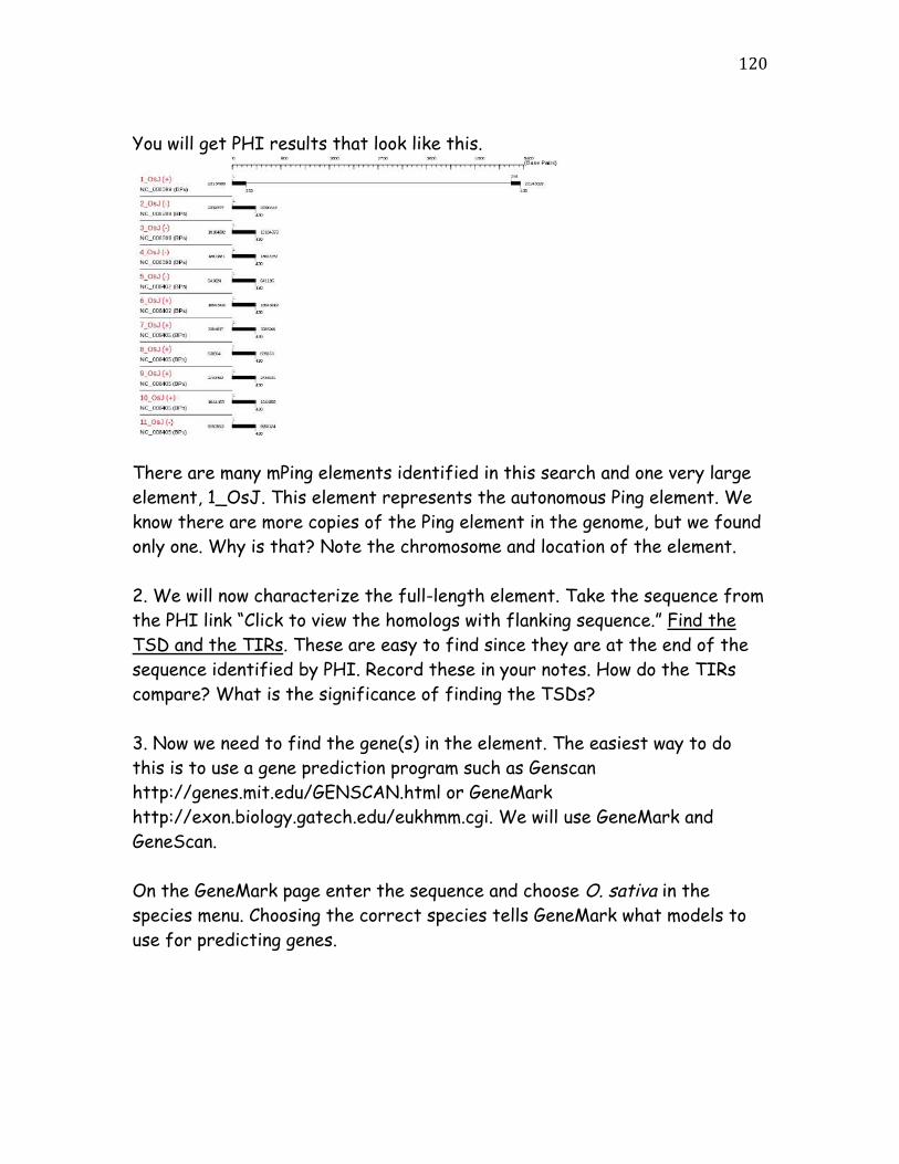
120
You will get PHI results that look like this.
There are many mPing elements identified in this search and one very large element, 1_OsJ. This element represents the autonomous Ping element. We know there are more copies of the Ping element in the genome, but we found only one. Why is that? Note the chromosome and location of the element. 2. We will now characterize the full-length element. Take the sequence from the PHI link “Click to view the homologs with flanking sequence.” Find the TSD and the TIRs. These are easy to find since they are at the end of the sequence identified by PHI. Record these in your notes. How do the TIRs compare? What is the significance of finding the TSDs? 3. Now we need to find the gene(s) in the element. The easiest way to do this is to use a gene prediction program such as Genscan http://genes.mit.edu/GENSCAN.html or GeneMark http://exon.biology.gatech.edu/eukhmm.cgi. We will use GeneMark and GeneScan. On the GeneMark page enter the sequence and choose O. sativa in the species menu. Choosing the correct species tells GeneMark what models to use for predicting genes.

121
GenScan set up is the similar but choose Arabidopsis. 4. The results are shown below:

122
GenScan output
GeneMark predicted three genes, and GenScan predicted two. Now we need to determine the identities of these sequences. 5. Find out what the genes are by using a blastp at NCBI on the Nucleotide Collection limited to rice. You will have to do some digging to find out the identities of some of the genes.

123
GeneMark gene 1 has very few hits in the database is it is likely that it is not an expressed gene. This is also supported by the fact that GeneScan did not predict the gene. A blastp with GeneMark gene 2 or Genscan gene 1 produces similar results. If you scroll through the results you will find GenBank submissions that support this gene being ORF1. GeneMark gene 3 and GeneScan gene 4 are the easiest and turn out to be TPase. Finding other family members So you now have a fully characterized Ping element. How would you use this element to find other TE family members? There are a few tools you will need to learn to do this. Get a Subsequence from a longer sequence. Use the Fasta Formatter on TARGeT to get a subsequence by entering the start and stop positions in the appropriate boxes.

124
Find direct or inverted repeats. Use Blast2Sequences to find repeats. You will need to use the sequence of the mPing TIR to find the Ping TIR in the Blast2Sequences results. 1. Enter the sequence into each textbox. For the Query sequence input the Query subrang of 1-3000 and in the Subject subrange of 6000-9000. These limits are guesses of where the TEs will be.
2. Change the program from “megablast” to “blastn” (Somewhat similar sequences (blastn)) in “Program Selection” portion of the page. Because the repeats of many DNA TE families are short we need to modify the “word size” parameter of blast from the default to 28 to 7. In order to get the lowest possible word size you need to first choose blastn.

125
3. Click the “Algorithm parameters” link and change the word size to 7.
There are three repeats identified by blast2sequences. The first and third are indirect repeats; the limits of the Query go up while the limits of the Subject decrease. The second hit is a direct repeat. Which repeat is the TIR of the element?
Click Here

127
A visual assay for the movement of rice TEs in Arabidopsis thaliana
Let’s re-state the problem we face here. We need to create an experimental system that mimics the one used by McClintock with TEs inserted into pigment genes and expressed in the kernel. For this experiment, we need to use a visual assay to test for movement of the rice mPing element in Arabidopsis. Creating a visual phenotype: You know what a reporter is—someone who goes out, gathers facts, brings back information, and turns it into ordered and accessible information. Just so, scientists use so-called reporter genes to attach to another gene of interest in cell culture, animals, or plants. Certain genes are chosen as reporters because the characteristics they confer on organisms expressing them are easily identified and measured. Most reporter genes are enzymes that make a fluorescent or colored product or are fluorescent products themselves. Among the latter kind is one that is central to your work this semester, called Green Fluorescent Protein or GFP. GFP comes from the jellyfish Aequorea victoria and fluoresces green when exposed to blue light. Researchers have found GFP extremely useful for an important reason: visualizing the presence of the gene doesn’t require sacrificing the tissue to be studied. That is, GFP can be visualized in living organisms by using fluorescent-imaging microscopy. The importance of the GFP reporter gene to modern science was evident when the 3 scientists responsible for its discovery and adaptation to the lab were awarded the 2008 Nobel Prize in Chemistry. You can learn more about this at this site: http://nobelprize.org/nobel_prizes/chemistry/laureates/2008/press.html In our experiments, the GFP reporter gene will substitute for the maize pigment gene. The mPing element has been engineered into the GFP gene so

128
that it cannot produce fluorescent protein. If mPing excises the GFP gene will be able to function again. Arabidopsis thaliana
In your previous biology classes you have certainly discussed model organisms and their desirable features. Model organisms include E.coli, yeast (Saccharomyces cerevisiae), Drosophila melanogaster, Caenorhabditis elegans (a.k.a. the worm), mouse (Mus musculus), and Arabidopsis thaliana. Like the other model organisms, A.thaliana is easily transformed by foreign DNA and is small and has a relatively short generation time (~6 weeks). This small flowering plant is a genus in the family Brassicaceae. It is related to cabbage and mustard. A. thaliana is one of the model organisms used for studying plant biology and the first plant to have its entire genome sequenced (~125 Mb, about the same as Drosophila).

129
Agrobacterium tumefaciens: introducing foreign DNA into plants.
In 1977, two groups independently reported that crown gall is due to the transfer of a piece of DNA from Agrobacterium into plant cells plants (Mary Dell Chilton, a postdoctoral associate at the University of Washington, and two other researchers working in Germany named Marc Van Montagu and Jeff Schell). This resulted in the development of methods to alter Agrobacterium into an efficient delivery system for gene engineering in plants. In short, Agrobacterium contains a plasmid (the Ti-plasmid) that contains a fragment of DNA (called T-DNA). Proteins encoded by the Ti-plasmid facilitate the transfer of the T-DNA into plant cells and ultimately, insertion into plant chromosomes. As such, the Ti-plasmid and its T-DNA is an ideal vehicle for genetic engineering. This is done by cloning a desired gene sequence into the T-DNA that will be inserted into the host DNA by Agrobacterium. As shown in the figure below, foreign DNA is inserted in the lab into the T-DNA (shown as the green DNA in the “cointegrate Ti plasmid below), which is then transformed into Agrobacterium, which is then used to infect cultured tobacco cells. The Ti plasmid moved from the bacterial cell to the plant nucleus where it integrated into a plant chromosome. Tobacco cells can be easily grown into “transgenic” plants where all cells contained the engineered T-DNA.
A crown gall tumor. Infection by the bacterium Agrobacterium tumefaciens leads to the production of galls by many of plant species.

130
The foreign DNA inserted into the T-DNA included both a gene of interest and a “selectable” marker, in this case, an antibiotic resistance gene. This is necessary because the procedure for transferring a foreign DNA into a plant via Agrobacterium-mediated transformation is very inefficient. By using media/agar containing the antibiotic, only the cultured cells with the T-DNA in their chromosomes will be resistant to the antibiotic and able to grow.
Back to Ping and mPing: how they were discovered.
Isolating Ping and mPing from rice (refer back to figure 7, page 7) : Geneticists had never isolated an active TE from rice like the Ac and Ds elements discovered by Barbara McClintock in maize. The logic used to isolate the first active rice TEs, Ping and mPing, is described.
Rice (Oryza sativa) has the smallest genome of all cereal grasses at 450 million base pairs (Mb). By contrast, the maize genome is almost six times larger at 2500 Mb. About 40 percent of the rice genome comprises repetitive DNA and most of this is derived from TEs. As discussed above, most of the TEs in a genome are inactive due to mutation. Because the full genome sequence for rice is known, members of the Wessler lab were able to use a computational approach to identify TEs that were potentially active based solely on their sequence characteristics. To find an active TE in rice, researchers compared the publicly available genome sequence of rice to itself. This sounds confusing, but here is what it means: Scientists first used computers to compare the genome sequence of Oryza sativa (domesticated rice) to itself and identified several sequences
Schematic of how Agrobacterium has been exploited to deliver foreign DNA into plant chromosomes.

131
that were repeated (called families or repeats). The repeat families were then analyzed (by computer again) to identify families that contained identical or almost identical sequences. The researchers reasoned that actively moving TEs should be represented by several identical or nearly identical copies in a genome. The reason for this is that when an element moves, an identical copy inserts elsewhere in the genome. Over millions of years these originally identical copies accumulate mutations (more on this later) and start looking different. By analyzing the genome this way, the researchers found a 430bp sequence with 50 nearly identical copies scattered across the 12 rice chromosomes. They named it “mPing” for “miniature Ping.” A note here about the precision of words that scientists use to describe experimental results. In this case, the researchers called mPing a “candidate” for an active transposon” and not simply an “active transposon.” The reason is that computational analysis usually identifies sequences that must be tested further by experiments. In other words, finding identical copies of a TE in a genome is not sufficient evidence to conclude that mPing is in fact an active element. In Experiment 1 you will test whether mPing is actually able to move - right before your eyes. It was puzzling to understand how mPing could transpose because it is very small and does not code for any proteins and is thus unable to move on its own. The researchers reasoned that there must be a protein-encoding transposon in the rice genome that encodes the transposase necessary to enable itself and other related elements to move. To find this coding element, the researchers searched the rice genomic sequence for longer related elements. They found a candidate TE which they called Ping - that had the same ends as mPing but was much longer (~5000 bp) and contained two ORFs. One encodes the transposase gene and the second (called ORF1) is of unknown function (see Figure 7, page 7). The purpose of thist experiment will be to test whether any or all of the proteins encoded by Ping can mobilize the mPing element. In other words, can either ORF1 or the transposase or both mobilize the mPing element.

132
Design of the experiment and controls
Now up until this point Ping and mPing were considered active TE candidates, - as there was no evidence that these TEs were actually capable of moving around nor was there evidence that Ping produced a proteins that could catalyze the movement of mPing. Experimental evidence was necessary to move these elements from candidates to bona fide active TEs. To address these questions, transgenic Arabidopsis plants were generated by engineering T-DNA in the test tube and using Agrobacterium tumefaciens to deliver the following constructs into Arabidopsis plants. These are described in detail below.

133
In this experiment we are testing whether the Ping encoded protein(s) can catalyze the transposition of mPing. So, there are actually three questions we will be attempting to answer:
--Can ORF1 protein by itself excise (move) mPing? --Can Tpase protein by itself move mPing? --Can both proteins work together to move mPing? To address these questions you will analyze mPing excision in transgenic Arabidopsis plants containing one or two of the following T-DNA constructs:

134
(A) Plants containing this T-DNA in their genome are the positive control. These plants should be green under UV light because the GFP protein is produced (designated GFP+).
(B) Plants containing this T-DNA in their genome are the negative control. These plants should be red under UV light because there is no GFP protein (designated GFP-). Note that the red color is due to chlorophyll fluorescence.
(C) Plants with this T-DNA are part of your experimental unknown.
(D) Plants with this T-DNA are also part of your experimental unknown.
(E) Not shown – NO T-DNA at all. This is the wild type control.
Note that A and B have the same antibiotic resistance gene and C and D share a different one.
The transgenic Arabidopsis plants used in this experiment contain one or two of the 4 T-DNA insertions in their genome.

135
A closer look at the regions that will be amplified in the experiment The regions to be amplified by PCR in this experiment are shown below as arrows to indicate the PCR primers and the direction of DNA synthesis. Once you have grown your Arabidopsis seedlings, you’re ready to isolate leaf DNA and to do PCR.

136
Examination of mPing excision from A. thaliana leaf DNA Overview: In this experiment you will test the hypothesis that the Ping element of rice produces one or two proteins (transposase plus ORF1 protein) that can catalyze the excision the mPing element in the model plant Arabidopsis thaliana. In part I, you will examine phenotypes of A. thaliana leaves and in part II you will extract DNA from the leaves of three different strains and set up your PCR amplification. Protocol: You will work in groups of two. Each group will analyze a full set of plants.
I. Plating of Arabidopsis seeds. One to two weeks before actually doing PCR with leaf DNA, the instructors will start growing the plants we will use in this experiment by plating Arabidopsis seeds on petri dishes containing the antibiotic kanamycin and MS salt media. Plate means more or less the same thing as plant, except in a petri dish. The plates were put into a growth chamber where they germinated for ~5 days. The reason that you will not be doing this part of the experiment is because it is very easy for a novice to contaminate the plates with bacteria and/or fungus. II. Examine leaves under microscope. You will view and photograph the seedling under a microscope using visible and UV light. III. Extract genomic DNA from seedlings. Nucleic acids are extracted from the seedlings using a simple protocol. After you extract genomic DNA you will visualize it on an agarose gel. You will use the standard DNA extraction protocol with one modification. Because there is so little tissue you will grind the tissue in the 1.5 ml tube. This will be demonstrated in class.

137
IV. Amplify genomic DNA using PCR. Today you will amplify the DNA using 3 pairs of primers: one pair for GPF, one pair for ORF1, and one pair for Tpase. The primers for ORF1 and Tpase will be mixed and used in a single PCR reaction. This is called duplex PCR. For each group, one person should set up the GFP PCRs and the other should set up the ORF1+Tpase reactions. Each person will have six DNA samples to analyze. We also need an additional negative control that will be water in place of DNA, giving you seven reactions in total. You need to make a master mix of eight reactions to make sure you have enough for the seven tubes. Pour a 1.5% gel for each group. After everyone is done, your samples will be cycled with the following conditions:
1 cycle for: initial denaturation 94°C 3 min 30 cycles for: denaturation 94°C 30 sec
annealing 58°C 30 sec extension 72°C 1 min
1 cycle for: final extension: 72°C 10 minutes Sequences of the Primers used: GFP Primers (772 and/or 339 bp amplimers) GFP-R 5’- AGA CGT TCC CAA CCA CGT CTT CAA AGC -3’ GFP-F 5’- CCT CTC CAC TGA CAG AAA ATT TGT GC -3’ ORF 1 Primers (239 bp amplimer)
ORF1-FOR 5'- CAC TGG TCA AGG TTG AAG TCA GCG ATC TCT G -3' ORF1-REV 5'- CAG CAT CCA TTT CGC TCT TGT CTT TCT CTG -3'
Tpase Primers (435 bp amplimer)
TPase-For 5'- GGT ATG TTC GGT AGC ATT GAC TGT ATG CAT TGG C -3' TPase-REV 5'- GAA TCG ACG TTG TAG AAC ACC AAA TGC TCT CTC -3'

Tracking epigenetic silencing of a transposon in maize.Damon Lisch, U.C. Berkeley
Overview: As you have seen in class, transposons can reach very high copy numbers, to the extent that some genomes are mostly transposon. However, the hosts are not without resources to counter these selfish elements. Over the past few years, we have become aware of an anxcient immune system whose function is to recognize and silence transposons and invading viruses. It does so by recognizing particular forms of RNA
that are produced by transposons but not by most host genes. One powerful trigger is double-stranded RNA (dsRNA). Transposons are particularly prone to produce double stranded RNA. They move from place to the place within the genome and can cause a variety of genomic rearrangements - events that can produce aberrant transcripts, including antisense and hairpin RNAs such as the ones portrayed above. Antisense transcripts can anneal with mRNAs to produce dsRNA. Hairpin RNAs are stretches of RNA where one portion of the molecule is complementary to another part of the same molecule. Such RNAs can be produced if transcription proceeds through an inverted repeat, a common feature of some transposons (see above figure).
! 139

Once dsRNA is detected, it triggers a cascade of events that lead to the production of small interfering RNAs (siRNAs) that are used to target all complementary RNAs in the cell for degradation. As you will see in class, this is an effective way to eliminate all transcripts from a given transposon, and without transcript, autonomous transposons have no way of producing the enyzmes they need to transpose. In this process, the dsRNA produced by a given transposon acts an “antigen” that triggers an immune response. However, the system is actually smarter than that, because it also includes a system that “remembers” who the transposon was, even after the trigger is lost. This memory system involves modification of cytosine nucleotides by the addition of a methyl group (DNA methylation), as well as modification of histones (which can change chromatin density). These modifications force the transposon to produce a form of aberrant RNA that continues to trigger silencing, even after the initial trigger is gone. These modifications will be described in more detail in class on tuesday.
Today we will be examining the genetic segregation of a DNA sequence that acts as a trigger of transposon silencing in maize. The focus of our
experiments will be members of the Class II superfamily Mutator. The Mutator system was discovered in maize in the 1970s. It got its name because it is highly mutagenic and prone to increase its copy number rapidly. The system is composed of non-autonomous elements (or several
! 140

types, called Mu1 through Mu8) and an autonomous element, MuDR. The non-autonomous elements only jump when MuDR is present. In our example, a non-autonomous element is inserted into a gene required to make color in the maize seed. When MuDR is present, the non-autonomous element (Mu1.7 in this case) jumps out of the color gene late during development of the seed. The result is small spots of revertant (wild-type) colored tissue on a mutant background. These spots of color serve as a powerful assay for the presence of an active MuDR element in the genome of that plant. Further, the frequency of spotting can indicate how active MuDR is in a given kernel. We will use this fact to track transposon inactivation in our families.
Classical genetic analysis:In order to understand our experiment we need to understand basic classical genetic analysis. The figure to the right illustrates a cross. At the top, each parent carries two homologous chromosomes; one from each parent. These are indicated by the parallel lines. MuDR is indicted by the triangle inserted into one of the lines. This plant is heterozygous for the insertion, since only one homologous chromosome has it. Below the cross are the
! 141

progeny, with the expected genotypes laid out in a grid. To the left of the blue box are the possible genotypes in the egg of the female. Because of the principle of random assortment, each product of meiosis has an equal probability of getting one or the other homologous chromosome. Thus, half of the eggs in the female in this cross will get MuDR and half will not. Above the blue box are the expected genotypes of the pollen. Note that the male parent only contributes pollen that lacks MuDR. Inside the blue box are the expected progeny classes, which we get by combining the various egg and pollen genotypes. As we can see, when a plant that is heterozygous for a single MuDR element is crossed to a plant that doesn’t carry MuDR, half the progeny will carry MuDR and half don’t, because half of the eggs receive MuDR and half do not. The result is an ear that segregates 50% spotted kernels. As we will see below, plants grown from these kernels can be genotyped for the presence or absence of MuDR.
Epigenetic silencing of the Mutator System:Silencing of the Mutator transposon system can be triggered by a rearranged version of MuDR called Mu killer (Muk). Mu killer is a version of MuDR in which half the element has been duplicated and inverted relative to itself, resulting in a mirror image, similar to the TIRs that are associated with many transposons, only much longer. Transcription from a
! 142
amy4 acm1
Muk
AAAA1 kb

nearby promoter (the acm1 gene) results in transcription all the way through this mirror image of part of a MuDR element. The resulting transcript has a hairpin - RNA sequences that compliment each other, just like the two strands of DNA compliment each other. In the figure to the right, the transcript produced by Mu killer is illustrated. Transcription proceeds from a flanking promoter, through the mirror image version of MuDR and is polyadenylated (AAAA) at a flanking site. Polyadenylation permits export of this RNA to the cytoplasm. The resulting RNA transcript includes parts of two flanking genes as well a the MuDR hairpin. The double stranded RNA portion of this transcript (which corresponds to MuDR) is processed into siRNAs. As will be discussed in class, this
double-stranded RNA is processed by a dicer into siRNAs, which cause subsequent cleavage of normal MuDR transcripts and eventual transcriptional silencing of MuDR elements. When a plant carrying MuDR
! 143

is crossed to a plant that is heterozygous for Muk, the result is an ear that segregates for MuDR and Muk. The figure above shows the genetic composition of the two parents and the resulting progeny based on genetic principles. One parent carries MuDR as a heterozygote, and the other carries Mu killer as a heterozygote. Note that the two elements are on different chromosomes, as indicated by the black and purple lines. When the female parent undergoes meiosis, half the eggs carry MuDR, and half lack it; none of them carry Muk. Similarly when the male parent undergoes meiosis, half the pollen carry Muk, and half lack it. Each of four possible combinations are possible in the progeny. Thus, the resulting progeny kernels segregate 25% MuDR with Muk, 25% with MuDR without Muk, 25% Muk alone and 25% neither MuDR nor Muk. The resulting ear looks like the picture to the right. Notice the weakly spotted kernels. These are individuals that inherited both MuDR and Muk. In these kernels, MuDR transcript is being degraded because Muk produces the trigger, or antigen, that causes dicer-mediated degradation of MuDR transcript. What happens next is even more interesting, because it shows that the plant can remember that an element has been targeted for silencing in a previous generation. The cross described above produces a class of weakly spotted kernels that carry MuDR and Mu killer. When plants grown from these kernels are crossed to a tester (a plant with neither MuDR nor Muk), nearly all of the resulting kernels are non-spotted, even the plants with MuDR and without Muk.
The cross is illustrated on the next page. A plant carrying MuDR and Muk is crossed to a plant lacking both MuDR and Muk. Note that genetic segregation of these elements should (and does) produce a class of progeny that carries MuDR but that lacks Muk. The female parent can produce four kinds of eggs, representing each combination of MuDR and Mu killer. The tester produces one kind of pollen. Thus, there are four different kinds of progeny, each with an equal probability. Note the class of progeny that carries MuDR but lacks Mu killer. If MuDR is effected only
! 144

when it is exposed to Muk, then we would expect that once Muk is lost, MuDR should regain activity. But it does not, as is indicated by the fact that
! 145

the kernel is not spotted. The progeny of these plants can be propagated indefinitely, and MuDR never wakes up again. Thus the genome “remembers” that MuDR was silenced, even after the trigger, or antigen, Muk, is lost. It’s important to note, however, that the DNA sequence of the MuDR element is identical to when it was active. Thus, the element is only sleeping, not dead. One note on classical genetics. Although it can be confusing, it is also remarkably powerful because it can give clean elegant answers to very complicated problems. Indeed, geneticists use the acronym “APOG” to describe how useful it can be - ask Damon what it stands for.
Experimental Protocol:
In this laboratory, we will examine the genetic segregation of MuDR and Muk to examine the effects of Muk on MuDR. In order to do this we will first need to extract DNA from sprouts grown from corn kernels. The extraction protocol is provided on a separate hand-out. The protocol is relatively straight-forward. First we will grind up the tissue in liquid nitrogen, which makes grinding easier and breaks up the cells and cell walls. Next, we will add a buffer, basically salty water EDTA, which inhibits enzyme activity (we don’t want our DNA chewed up by nucleases). Then we will add SDS, which is a concentrated surfactant, or soap, which pops open cell and nuclear membranes (that’s why “antibacterial” is such a rip off - soap is plenty antibacterial all by itself). Then we heat to 65˚ C. This dissociates protein complexes and allows everything to mix well. Then we add potassium acetate. This causes the proteins, but not the DNA, to precipitate out of solution. After chilling for a few minutes (to aid in protein precipitation) we spin the mix in a centrifuge, which separates the protein and assorted cell debris from the liquid that still contains the DNA. Then we suck off the liquid, leaving behind the debris, and add it to a new tube. Then we add an equal volume of isopropanol. This causes the DNA to precipitate out of solution. Depending on the amount of DNA, we may see fine strands of it at this stage (this is the fun part). Then we spin the DNA down to the bottom of the tube, pour off the liquid, and re-suspend the DNA in water. Now it’s ready for analysis.
After extracting the DNA, we want to find out who has MuDR and who has Muk. To do this we will use PCR, which can specifically identify MuDR and Muk. It can do this because each of these elements is at a unique position in the maize genome. Thus, although the sequences of MuDR and Muk
! 146

are identical, sequences flanking those elements are unique. We will use PCR primers specific to MuDR at a particular position (p1) and primers specific to Mu killer. In each case, one primer will be specific to the transposon and one will be specific to the DNA sequence into which the transposon is inserted. Amplification will only work if the element (MuDR or Muk) is present at a particular position. If the element is not at that position, or is missing altogether, there will be no product.
Step1: DNA extraction. First we will obtain leaf tissue from plants grown from kernels with the various genotypes described above. Then we will extract the DNA using the protocol provided. After the DNA extraction we will have about 50µl of DNA in a series of 1.5 ml centrifuge tubes.
Label each tube with a name for the particular family being examined, the class of kernel (H for heavily spotted, W for weakly spotted and P for pale, or no spots) and a number for the individual plants. Put your initials on the side of the tube as well. Remember that none of the results will make sense later if you don’t label the tubes clearly. If you think you might have contaminated a tip, go ahead and throw it away.
! 147

Step 2: PCR genotyping.
As described above, we are interested in using PCR to genotype each individual from families segregating for MuDR and Mu killer. First we will examine the progeny of the following cross:
MuDR(p1)/- ; -/- x -/- ; Muk/-.
This is a cross between a plant that is heterozygous for MuDR at a particular position (p1) with a plant that is heterozygous for Mu killer. Seeds derived from the above cross have been separated into classes for you based on excision frequency (heavy, weak, pale). As we have seen, Muk acts on MuDR to reduce its activity, resulting in weakly spotted kernels. Thus, we will expect to find that plants grown from kernels with many spots will carry MuDR without Muk, and plants grown from weakly spotted kernels will carry both MuDR with Muk. Pale kernels should lack MuDR, but half of them should have Muk. We have grown sprouts from heavily spotted kernels, weakly spotted kernels and pale kernels from this cross.
Next we will examine progeny of the cross:
MuDR(p1)/-; Muk/- x tester (-/- ; -/-)
Recall that the plant carrying MuDR(p1) and Muk (MuDR(p1)/-; Muk/-) was derived from the cross between MuDR(p1) and Muk. This plant was grown from one of the weakly spotted kernels. The plant was then crossed to a tester that lacked both MuDR and Mu killer. Here, nearly all of the progeny kernels were pale. However, as described earlier, 25% of the progeny of this cross should carry MuDR without Muk. As before, we will genotype for MuDR(p1) and Mu killer. If there is a class of kernels that carries MuDR without Mu killer and that remained pale (no MuDR activity), then we will concluded that the genome is remembering to keep MuDR inactive even after Mu killer has segregated away.
As was done in a prior experiment, you will be resolving PCR products by agarose gel electrophoresis.
! 148
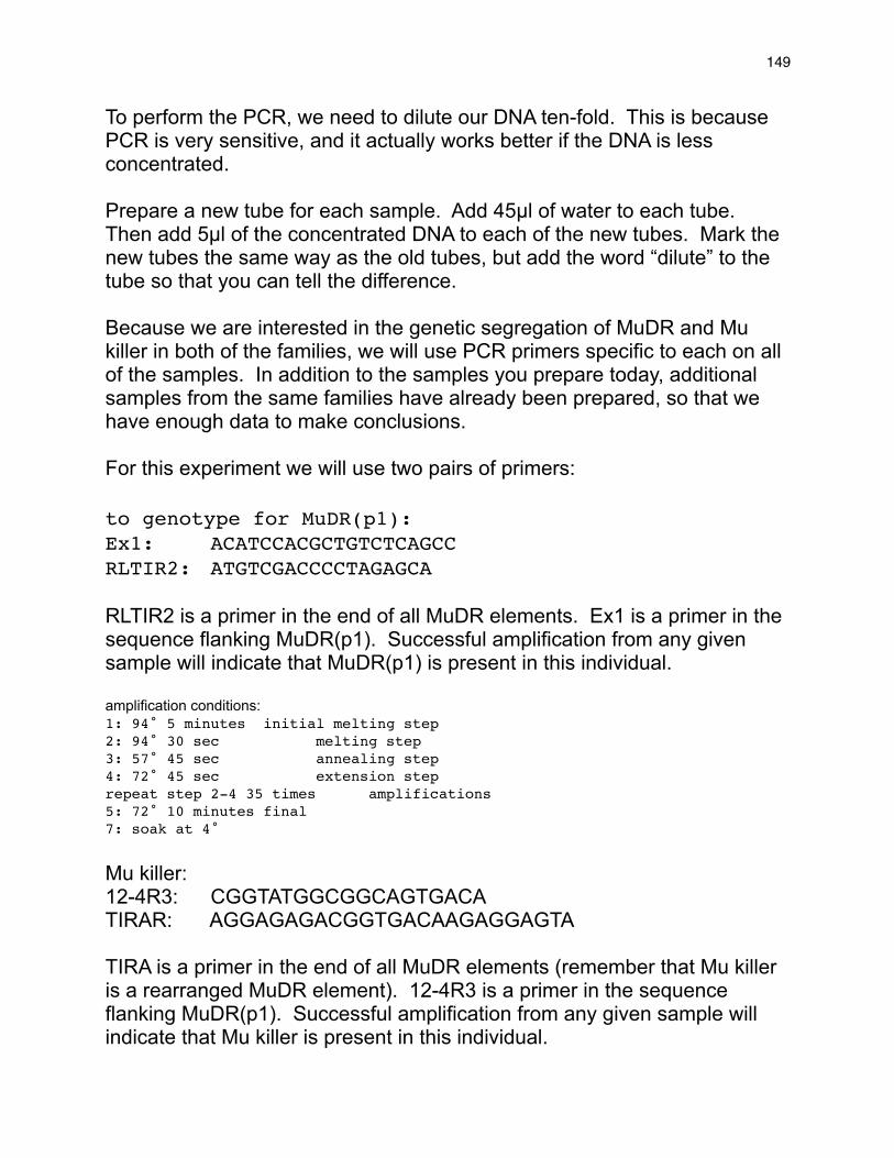
To perform the PCR, we need to dilute our DNA ten-fold. This is because PCR is very sensitive, and it actually works better if the DNA is less concentrated.
Prepare a new tube for each sample. Add 45µl of water to each tube. Then add 5µl of the concentrated DNA to each of the new tubes. Mark the new tubes the same way as the old tubes, but add the word “dilute” to the tube so that you can tell the difference.
Because we are interested in the genetic segregation of MuDR and Mu killer in both of the families, we will use PCR primers specific to each on all of the samples. In addition to the samples you prepare today, additional samples from the same families have already been prepared, so that we have enough data to make conclusions.
For this experiment we will use two pairs of primers:
to genotype for MuDR(p1): Ex1:!! ACATCCACGCTGTCTCAGCC!RLTIR2:! ATGTCGACCCCTAGAGCA
RLTIR2 is a primer in the end of all MuDR elements. Ex1 is a primer in the sequence flanking MuDR(p1). Successful amplification from any given sample will indicate that MuDR(p1) is present in this individual.
amplification conditions:1: 94˚ 5 minutes! initial melting step2: 94˚ 30 sec! ! melting step3: 57˚ 45 sec! ! annealing step4: 72˚ 45 sec! ! extension steprepeat step 2-4 35 times! amplifications5: 72˚ 10 minutes final 7: soak at 4˚
Mu killer:12-4R3: CGGTATGGCGGCAGTGACATIRAR: AGGAGAGACGGTGACAAGAGGAGTA
TIRA is a primer in the end of all MuDR elements (remember that Mu killer is a rearranged MuDR element). 12-4R3 is a primer in the sequence flanking MuDR(p1). Successful amplification from any given sample will indicate that Mu killer is present in this individual.
! 149

amplification conditions:1: 94˚ 5 minutes2: 94˚ 30 sec3: 60˚ 45 sec4: 72˚ 1 minrepeat step 2-4 35 times5: 72˚ 10 minutes7: soak at 4˚
Set up a standard 25 µl PCR reaction for the DNAs that you extracted
! 150

Review of Crosses:
! 151

153
Exploring Alu polymorphism and human diversity.
Read the review paper by Cordaux and Batzer starting on page 691. Alu is an active class 1 element in primates and there are many polymorphic Alu insertions. A DNA polymorphism occurs when there is a difference between chromosomes at a given locus. The PV92 insertion is polymorphic for presence or absence. The insertion at the Yg locus occurred in an ancestor of the modern primates and all Chromosome 5s of humans have a Yg insertion. The Alu insertion at the 225 locus is polymorphic and also has SNP differences that created three different insertion alleles. These sequence polymorphisms result in KasI restriction sites in some 225 alleles but not others. We will take advantage of the restriction sites to distinguish between the three insertion alleles. Human genomic DNA Preparation using the QIAGEN DNeasy Blood and
Tissue Kit 1. Pipette 500 µl of sterile water in a 1.5 ml tube. 2. Collect cheek cells (buccal cells) using a Catch-All sterile swab. Rub the inside of each cheek 20 times. 3. Swirl the swab in the 500 µl of water. You will see the cells come off the swab and water will turn cloudy. 4. Pellet the cells by centrifuging the tube for 2 minutes at high speed. 5. Pour off the supernatant. 6. Pipette 200 µl of PBS in the tube. Vortex the tube to resuspend the cell pellet completely. 7. Add 20 µl of Proteinase K.
154
8. Add 200 µl AL and vortex briefly. Heat at 56˚C for 10 min. 9. Add 200 µl of Ethanol. Vortex. 10. Put sample on DNeasy Mini spin column. 11. Centrifuge at 6000g (8000 rpm) for 1 min. Discard flow-through. Note this is NOT maximum speed.The DNA is now bound to the white membrane in the spin column. 12. Place the spin column in a new collection tube. Pipette 500 µl AW1. Centrifuge at 6000g (8000 rpm) for 1 min. 13. Place the spin column in a new collection tube. Pipette 500 µl AW2. Centrifuge at maximum speed for 3 minutes. 14. Place the spin column in a 1.5 ml tube. Cut off the cap from the tube. Spin for an additional 3 minutes at maximum speed. 15. Place the spin column in a 1.5 ml tube. Pipette 200 µl of Buffer AE onto the white membrane. Incubate at RT for 1 min. Spin at 6000g (8000 rpm) for 1 min. The DNA is eluted from the membrane and is now in solution. Measure the DNA concentration using the Nanodrop. For the Alu experiment you will amplify three different regions: Yg, 225, and PV92. You will need a 50 µl reaction for 225 and 25 µl reactions for Yg and 225. Also the PV92 primers require conditions that differ from Yg and 225 so keep them separate. QIAquick PCR Purification Protocol 1. Add 5 volumes of Buffer PB to 1 volume of PCR. Mix by inverting. If you have a 50 µl PCR you will add 250 µl of PB. 2. Pipette all liquid to a lilac colored spin column.

155
3. Centrifuge column at top speed for 60 secs. During the spin the PCR products will bind to the column. The primers and primer dimmers do not bind. 4. Discard the flow through. Pipette 750 µl of PE to the column. Spin again. 5. Discard the flow through. Spin agin. 6. Put column in a 1.5 ml tube. Add 30 µl of EB to the column. Wait 1 minute. 7. Spin in centrifuge at top speed for 1 min. Throw away the column. The PCR products are in the 1.5 ml tube. Keep this. BanI or KasI digestion: To the 30 µl recovered from the clean up add: Keep the enzyme on ice! 10X Buffer 4 3.5 µl 100X BSA 0.5 µl BanI 1.0 µl The total will be 35 µl. Incubate the reaction at 37˚C for 1 hour. Pour a 3% gel.

156
Digestion Pattern for S1 Digestion Pattern for S2
Sizes S1 S2 L No Alu 239 229 ---- ---- 146 219 ---- ----
Restriction Fragments
(bp) 73 ---- ---- Total Size
(bp) 458 448 474 135
Alignment 225F S1/1-458 GAGTCCAGCCCATTTTAGCATGGGACATTGAGTATGTTTTCATAACTGTTATCAAGAAGT S2/1-448 GAGTCCAGCCCATTTTAGCATGGGACATTGAGTATGTTTTCATAACTGTTATCAAGAAGT L/1-474 GAGTCCAGCCCATTTTAGCATGGGACATTGAGTATGTTTTCATAACTGTTATCAAGAAGT V 73 S1/1-458 ATTTTTATGCCGGGCGCCGTGGCTCACGCCTGTAATCCCAGCACTTTGGGAGGCCGAGGC S2/1-448 ATTTTTATGCCGGGTGCAGTGGCTCACGCCTGTAATCCCAGCACTTTGGGAGGCCGAGGC L/1-474 ATTTTTATGCCGGGTGCAGTGGCTCACGCCTGTAATCCCAGCACTTTGGGAGGCCGAGGC S1/1-458 GGGTGGATCATGAGGTCAGGAGATCGAGACCATCCTGGCTAACAAGGTGAAACCCCATCT S2/1-448 GGGTGGATCATGAGGTCAGGAGATCGAGACCATCCTGGCTAACAAGGTGAAACCCCGTCT L/1-474 GGGTGGATCATGAGGTCAGGAGATCGAGACCATCCTGGCTAACAAGGTGAAACCCCGTCT 224 S1/1-458 CTACTAAAAATACAAAAAATTAGCCGGGCGCGGTGGCGGGCGCCTGTAGTCCCAGCTACT S2/1-448 CTACTAAAAATACAAAAAATTAGCCGGGCGCGGTGGCGGGCGCCTGTAGTCCCAGCTACT L/1-474 CTACTAAAAATACAAAAAATTAGCCGGGCGCGGTGGCGGGCACCTGTAGTCCCAGCTACT S1/1-458 TAGGAGGCTGAGGCGGGAGAAGGGCGTGAACCCGGGAAGCGGAGCTTGCAGTGAGCCGAG S2/1-448 TAGGAGGCTGAGGCGGGAGAAGGGCGTGAACCCGGGAAGCGGAGCTTGCAGTGAGCCGAG L/1-474 TAGGAGGCTGAGGCGGGAGAAGGGCGTGAACCCGGGAAGCGGAGCTTGCAGTGAGCCGAG V S1/1-458 ATCGCGCCACTGCAGTCCGCAGTCCGGCCTGGGCGACAGAGCGAGACTCCGTCTC----- S2/1-448 ATCGCGCCACTGCAGTCCGCAGTCCGGCCTGGGCGACAGAGCAAGACTCCGTCTC----- L/1-474 ATCGCGCCACTGCAGTCCGCAGTCCGGCCTGGGCGACAGAGCAAGACTCCGTCTCAAAAA S1/1-458 ------------AAAAAAAAAAAAAAAAAAAAAAAGAAGTATTTTTATATGCTTCACACT S2/1-448 ----------------------AAAAAAAAAAAAAGAAGTATTTTTATATGCTTCACACT L/1-474 AAAAAAAAAAAAAAAAAAAAAAAAAAAAAAAAAAAGAAGTATTTTTATATGCTTCACACT S1/1-458 AATTAAAAGATGATAAAGTTTGATATGAGAAATTAAATGACATGTTTGTGCTGGG S2/1-448 AATTAAAAGATGATAAAGTTTGATATGAGAAATTAAATGACATGTTTGTGCTGGG L/1-474 AATTAAAAGATGATAAAGTTTGATATGAGAAATT-AATGACATGTTTGTGCTGGG 225R

157
Exploring MITE insertion sites using Transposon Display In this project you will explore the insertion sites of MITEs in rice and Arabidopsis. In rice we will focus on mPing a MITE that is actively transposing in several cultivated land races: 119, 123, and 157. Another MITE called Osmar5NA (NA = non-autonomous) was created from a Mariner-like TE found in rice. Osmar5NA was transformed into Arabidopsis along with the Osmar5 transposase. Osmar5NA is moving in the germline of Arabidopsis so we can look at insertions that accumulate during several generations of plants. A technique called transposon display was developed to amplify many MITE insertions from genomic DNA at one time. To do this we have to use a trick called adapter ligation. We know that one end of the PCR fragments will be the TE (mPing or Osmar5), but we do not know the other end (that is what we are trying to find out). For this technique to work, we must supply a second PCR priming site. To do this we first restriction digest the genomic DNA with the enzyme BfaI or MseI (see figure). BfaI cuts the sequence CTAG between the C and the T. MseI cuts TTAA between the T and the A. After digestion we know that the DNA fragments will end in TA. So we can ligate a synthetic piece of DNA, called the adapter, that has the complementary overhang of AT. We know the sequence of the adapter and will use it as the second PCR primer binding site.

158
After ligating the adapter we do the primary amplification (called pre-selective amplification in the figure). After the primary amplification there are too many amplimers and there are a lot of non-specific amplimers. We dilute the primary reaction and amplify a second time using a selective adapter primer. In this case we add one or two nucleotides on the 3’ end to reduce the number of priming targets. For mPing we have at least 10 individuals from 3 land races and we have several generations of Arabidopsis for Osmar5NA. The first step is to extract high quality genomic DNA. You will harvest only part of the plant and the plant will be grown and selfed to collect seeds.
TD Step 1: Extract Genomic DNA using DNeasy Plant Mini Kit. 1. Collect tissue. Grind to fine powder in mortar with liquid nitrogen. 2. Add 400 µl of Buffer AP1 and 4 µl RNaseA. Grind a little more and pour into 1.5 ml tube. 3. Incubate for 10 min. at 65˚C. 4. Add 130 µl AP2 to lysate. Mix and incubate 5 min on ice. 5. Centrifuge top speed fo 5 minutes. 6. Pipette lysate on QIAShredder spin column. Spin 2 min at top speed. 7. Place flow through into new 1.5 ml tube. 8. Add 1.5 volumes AP3. 9. Pipette 650 µl onto the DNeasy spin column. Spin 1 min. at 6,000xg. 10. Repeat 9 if there is left over sample. 11. Place column in new collection tube. Add 500 µl AW. Spin 1 min. at 6,000xg.

159
12. Pour out flow-through. Add 500 µl AW. Spin 2 min. at max speed. 13. Put column in new 1.5 ml tube. Spin 2 min. at max speed. 14. Pipet 100 µl of AE onto the spin column. Incubate RT for 5 min. Spin 1 min. at 6,000xg. 15. Repeat 14. Nanodrop your DNA samples to determine concentration and purity. Set up a PCR reaction with actin to check amplifibilty of the DNA.

161
Step 2: Restriction/Ligation (R/L) In this step you will digest the DNA with a restriction enzyme leaving ‘TA’ overhangs. In the same reaction you will ligate an adapter that has a complementary ‘AT’ overhang. This will provide a defined end so we can do PCR. You need to dilute the genomic DNA to 5 ng/µl. Do the calculations and dilute each of your samples. Adapter sequence: BfaI_Adp-For 5’-GACGATGAGTCCTGAG-3’ BfaI_Adp-Rev 5’-TACTCAGGACTCAT-3’ These two oligos were synthesized by IDT separately, but DNA Ligase requires double-stranded templates. To make the adapter double stranded the two oligos must be annealed. To do this they are mixed in an equal molar ratio and heated to 95˚C for 10 minutes. This ensures the oligos are completely single-stranded. The mixture is then allowed to cool slowly at room temperature for ~1hr. During the cooling step, the complementary strands find each other and hydrogen bond. The result should be a solution of annealed adapters: BfaI_Adp-For 5’-GACGATGAGTCCTGAG-3’ BfaI_Adp-Rev 3’TACTCAGGACTCAT-5’ DNA LIGASE IS EXTREMELY HEAT SENSITIVE. DO NOT EVER LEAVE IT AT ROOM TEMPERATURE. KEEP IT IN THE FREEZER BLOCK. MIX THE R/L REACTION ON ICE. The TD protocol is optimized for two restriction enzymes: BfaI and MseI.
Arabidopsis sample: BfaI Rice samples: MseI

162
Restriction/Ligation (R/L): X1 X10 X20 X50 ddH2O 16.5 165 330 825 NEB Buffer 4 5 50 100 250 Ligase Buffer 5 50 100 250 Adapter 1 10 20 50 BfaI or MseI 1 10 20 50 Ligase 1 10 20 50 BSA 0.5 5 10 25 DNA (5ng/µl) 20 Total 50 500 1000 2500 1. Determine the size of the master mix you require. Make the mix (on ice!). Add 30 µl of the mix to enough PCR strip tubes. 2. Add 20 µl of genomic DNA to the sample. 3. Incubate overnight @37°C. 4. Check for complete digestion by running 10-‐20µl on an agarose gel. 5. Dilute the remaining R/L 1:3 with H2O before proceeding to Primary Amplification. Step 3: Primary Amplification In this step, you will use PCR to amplify the sample. You will use one primer specific to TE we are interested in: mPing or OSmar5NA. The adapter primer will be specific to the restriction enzyme you used: BfaI or MseI. In primary (1˚) amplification the adapter primer is exactly the sequence of the adapter which provides little specificity. Arabidopsis: OsmarNAS_P1 5’-GTACAAATGCTGTAAATGACAGC-3’ BfaI+0 5’-GACGATGAGTCCTGAGTA-3’ Rice: mPing_P3 5’-GTAGCCGTGCAATGACACTAG-3’ MseI+0 5’-GACGATGAGTCCTGAGTA-3’
We will use Taq purchased from a different company so the PCR cocktail is different.

163
Primary Amplification (PA): X1 X10 X20 X50 ddH2O 10.3 103 206 515 10xBuffer 2 20 40 100 MgCl2 2 20 40 100 dNTPs (2mM) 2 20 40 100 BfaI/MseI+0 1 10 20 50 P1 Primer 1 10 20 50 Taq 0.2 2 4 10 DNA 1.5 Total 20 200 400 1000 Temp. Time #Cycles 72°C 2’ 1 94°C 3’ 1 94°C 45” 58°C 45” 72°C 45” 30 72°C 5’ 1 1. Determine the size of the cocktail you need and write it in your notebook. 2. Mix up the cocktail and distribute 18.5 µl/PCR tube. 3. Add 1.5 µl of the diluted R/L. 4. Cap and cycle the tubes as shown in the table. 5. Run 10µl on an agarose gel to make sure that amplification occurred (a smear from 100-‐800 bp should be seen). 6. Dilute the remaining PA 1:99 with H2O before starting the Secondary Amplification.
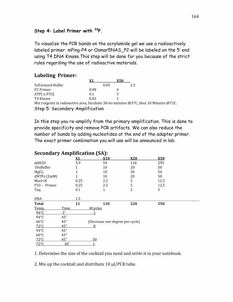
164
Step 4: Label Primer with 33P. To visualize the PCR bands on the acrylamide gel we use a radioactively labeled primer. mPing-P4 or Osmar5NAS_P2 will be labeled on the 5’ end using T4 DNA Kinase.This step will be done for you because of the strict rules regarding the use of radioactive materials. Labeling Primer: X1 X50 5xForward Buffer 0.05 2.5 P2 Primer 0.08 4 ATP[ γ-‐P33] 0.1 5 T4 Kinase 0.02 1 Mix reagents in radioactive area, Incubate 30-‐6o minutes @37C, then 10 Minutes @72C. Step 5: Secondary Amplification In this step you re-amplify from the primary amplification. This is done to provide specificity and remove PCR artifacts. We can also reduce the number of bands by adding nucleotides at the end of the adapter primer. The exact primer combination you will use will be announced in lab. Secondary Amplification (SA): X1 X10 X20 X50 ddH2O 5.9 59 118 295 10xBuffer 1 10 20 50 MgCl2 1 10 20 50 dNTPs (2mM) 1 10 20 50 MseI+N 0.25 2.5 5 12.5 P33 – Primer 0.25 2.5 5 12.5 Taq 0.1 1 2 5 DNA 1.5 Total 11 110 220 550 Temp. Time #Cycles 94°C 3’ 1 94°C 45” 66°C 45” (Decrease one degree per cycle) 72°C 45” 8 94°C 45” 60°C 45” 72°C 45” 30 72°C 30’ 1 1. Determine the size of the cocktail you need and write it in your notebook. 2. Mix up the cocktail and distribute 10 µl/PCR tube.

165
3. Add 1.5 µl of the diluted 1˚ rxn. 4. Cap and cycle the tubes as shown in the table. Step 5: Pour gel. For TD you must use an acrylamide gel. This type of gel has single base pair resolution. Acrylamide and bisacrylamide are covalently bonded into a very thin porous gel between two glass plates. Acrylamide is a neurotoxin so wear gloves when handling it. Assembly of the glass plates and the pouring of the gels will be demonstrated in class. You will then have the opportunity to pour your own gels. After the gel polymerizes: 1. Add 7µl of loading buffer and denature samples 5 min @ 95°C, chill on ice, and load 3µl. 2. Run samples 35mA constant for two hours and twenty mins. Loading, running, and drying gels will be done for you, while you watch.

167
Obtaining DNA sequence from PCR bands To obtain DNA sequence from the PCR band in a polyacrylamide gel you must re-amplify the band. To further ensure quality DNA sequencing reads we will clone the PCR bands into a bacterial vector called pCR2.1-TOPO using the TOPO-TA cloning kit. You will then need to purify the vector containing the cloned fragment. Re-amplify the PCR band with the following primers: Rice: MseI+GG and mPing-P4 Arabidopsis: BfaI+1 and OSmar_SA. Remove 18 µl of PCR from the strip tube and add 4 µl of loading dye. Run this on a 1.5% gel. Save the remaining PCR. If there is a single band in a lane then you will clone directly. If not you will need to extract the correct band from the gel.
Gel Extraction using the Qiagene Gel Extraction Kit 1. Weigh the gel slice in the tube. Add 3 volumes of Buffer QG to 1 volume of gel (100mg ~ 100µl). For example, add 300 µl of Buffer QG to each 100 mg of gel. 2. Incubate at 50°C for 10 min in a water bath (or until the gel slice has completely dissolved). To help dissolve gel, mix by inverting the tube every 2–3 min during the incubation. 3. After the gel slice has dissolved completely, add 1 gel volume of isopropanol to the sample and mix. For example, if the agarose gel slice is 100 mg, add 100 µl isopropanol. 4. To bind DNA to the column material, apply the sample to the QIAquick column and then spin at 13,000 rpm for 1 minute. The DNA is now in a high salt/non-polar solution. Under these conditions the DNA sticks to silica (the stuff in the column). The maximum volume of the column reservoir is 800 µl. For sample volumes of more than 800 µl, simply load again.

168
5. Discard flow-through and place QIAquick column back in the same collection tube.
6. Add 0.5 ml of buffer QG to QIAquick column and centrifuge for 1 min. Discard the flow through. This step is only required for directly sequencing.
7. To wash any impurities (EtBr and agarose) from the DNA, add 0.75 ml of Buffer PE to QIAquick column, let the column stand 3min and spin column at 13,000 rpm for 1min.
8. Discard the flow through and centrifuge for another 1 min at 13,000 rpm. IMPORTANT: This spin is necessary to remove residual ethanol (Buffer PE). 9. Place QIAquick column in a clean 1.5 ml microcentrifuge tube. 10. To elute DNA from the column, add 30µl water to the center of QIAquick membrane, leave column on bench for 2 min, and centrifuge the column for 1 min at 13,000 rpm. IMPORTANT: Ensure that the elution buffer is dispensed directly onto the QIAquick membrane for complete elution of bound DNA. The tube containing the eluted DNA will then be sent to the sequencing facility (Yujun will do this). The TOPO vector We will be using TOPO to clone the gel bands from the PCR, transform E. coli, let the transformed bugs grow overnight, purify plasmid from bacterial colonies and send these purified plasmids to the sequencing facility. The idea behind TOPO cloning, according to the company’s web site, is “to effectively clone DNA produced by a particular method (in your case, PCR) and to enable specific downstream studies (in your case, DNA sequencing).” The method works because Taq Polymerase adds “non-templated” A’s to the ends of PCR products. The vector is cut in a way so that there are T overhangs. An enzyme called Topoisomerase is used to ligate the vector to the PCR product.

169

170
TOPO TA cloning 1. Place tube of Top-10 competent cells and PCR2.1 TOPO vector on ice to thaw. 2. Add the following to a 1.5 ml microcentrifuge tube. Pipette gently and do not mix vigorously.
2 µl gel purified PCR product 2 µl H2O 1 µl salt solution 0.5 µl PCR2.1 TOPO Vector (add last)
3. Centrifuge 30 sec to collect reaction in bottom. Incubate for 10 min at room temperature (on your bench) 4. Transfer 2µl of the incubated mixture to the tube containing Top-10 competent cells (keep on ice). Pipette gently and do not mix vigorously. 5. Incubate the tube on ice for 20 min. (Only transformed E.coli cells can grow on LB selective plate. Furthermore, if X-gal is added, cells that have empty vectors will grow into blue colonies and they can be easily discerned from cells with “loaded” vectors, whose colonies will be white.) 6. Incubate in a water bath for 30 sec at 42oC. (This is called the heat shock - it is when DNA is actually taken up into the bacteria from the surrounding liquid) 7. Immediately place cells on ice for 1 min. 8. Add 200 µl SOC (or LB) medium (keep sterile). 9. Incubate in a 37oC shaker for 20 min. 10. Label the plates on the “bottom.” Pipette 150µl of bacterial solution onto one selective plate (work quickly to keep the plates closed as much as possible). Pour 3-5 sterile glass beads onto the plates, cover and shake horizontally to spread the liquid. Dump the glass beads.

171
12. Incubate the plates overnight in an incubator at 37oC
Growing up Your Bacterial Colonies Pick bacterial colonies that have inserts (the white colonies) into test tubes containing liquid medium and grow them overnight as described below. Take a picture of each plate for your lab notebook. A. Materials: 1. LB + Carb liquid growth medium (for growing bacteria) 2. Sterile toothpicks or pipette tips B. Protocol: 1. Add 3 ml of liquid growth medium (LB/Carb) into sterile test tubes 2. Using a sterile loop touch a single white colony from the agar plate and drop the toothpick (one per tube) into the test tube. 3. Incubate the test tubes in the spinner overnight at 37oC.
Plasmid Purification from Bacteria (Mini-Prep) 1. Transfer 1.0 ml of your E. coli sample from the overnight culture to a labeled 1.5ml centrifuge tube (put tip in bacterial waste container after use). 2. Cap and centrifuge for 3 min at 8,000 rpm. Decant (dump) supernatant into the bacterial waste. Repeat steps 1 and 2 one time. 3. Add 250µl buffer P1 and vortex to re-suspend the pelleted bacterial cells. No cell clumps should be visible after re-suspension of the pellet. 4. Add 250µl buffer P2 and gently invert the tube 4–6 times to mix. Do not vortex.

172
5. Add 350µl buffer N3 and invert the tube immediately but gently 4–6 times. The solution should become cloudy. 6. Centrifuge for 10 min at 13,000 rpm. A compact white pellet will form. 7. Pipet ~ 800µl of the supernatant (not the white precipitate) from step 4 and apply to a labeled QIAprep spin column. 8. Centrifuge for 30 sec. Discard the flow-through. 8a. Add 500 µl of Buffer PB. Centrifuge and discard the flow through. 9. Add 0.75 ml PE buffer and centrifuge for 1 minute. Discard the flow-through. 10. Centrifuge for an additional 1 min to remove residual buffer. 11. Transfer the QIAprep column to a clean labeled 1.5 ml centrifuge tube. 12. Add 100µl EB to the center of each QIAprep spin column, let stand for 1 min, and centrifuge for 1 min. 13. Discard the column (plasmid DNA will be in the liquid at the bottom of the tube). The black/white screening for plasmids (vectors) with PCR inserts is fairly accurate. To guarantee that the plasmid has a PCR insert we can digest the plasmid with the restriction enzyme EcoRI which cuts GAATTC. The TOPO vector was conveniently designed with the EcoRI sites on each side of the cloning site. You will digest each plasmid with EcoRI. Plasmid 2.0 10X Buffer 4 1.5 H2O 15.5 EcoRI 1.0 Total 20.0
Nanodrop the plasmid preps to determine their concentration. Preparing your samples for sequencing will be discussed in lab.

173
Analyzing DNA sequencing results Now that your DNA samples have been sequenced, you need to analyze the data. First you need to assess the quality of the data and then determine what the data mean. As you work on a sequence you must take notes about each step. Use a Google Docs to do this. Steps to assess the quality of the data: 1. Open the Genewiz website and login in: https://clims3.genewiz.com/default.aspx user: [email protected] password: 1503A
2. Click the tracking number 10-126801463.

174
3. Find your samples on the spreadsheet. I will explain the naming in class. 4. Find a sample were the QS (for quality score) and CRL (contiguous read length) are both in black. This sample is “high quality” according to the computer system. 5. Click on “View” in the Trace File column.
6. A new window will pop up. On the top will be the trace file and on the bottom will be the sequence. We will discuss this in class.
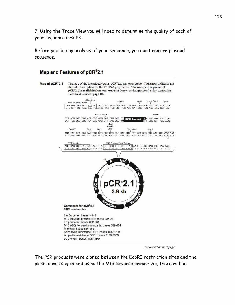
175
7. Using the Trace View you will need to determine the quality of each of your sequence results. Before you do any analysis of your sequence, you must remove plasmid sequence.
The PCR products were cloned between the EcoRI restriction sites and the plasmid was sequenced using the M13 Reverse primer. So, there will be

176
vector sequence on either side of the PCR insert. This sequence will interfere with analysis. There is a modified BLAST search that will compare your sequence to a database of plasmid vectors. This will show you what part of your sequence is vector and what part is interesting sequence. 1. Open the NCBI VecScreen web page. http://www.ncbi.nlm.nih.gov/VecScreen/VecScreen.html 2. Copy-and-Paste a sequence in the window and click “Run VecScreen.”
3. Click “View Report.”
4. The results graphic shows plasmid vector sequence in red or yellow and insert sequence in white.

177
5. In this case the insert sequence starts at 62 and ends at 172. 6. To extract this sequence open the web page: http://target.iplantcollaborative.org/fasta_formatter.html 7. Copy-and-Paste the complete sequence in the text field and enter the stat and stop numbers in the text boxes. Click “Format.”

178
8. Copy and paste the subsequence into your notes.
9. Now let’s think about what the sequence contains. Draw a diagram. 10. Identify the “known” portions of the sequence. BfaI adapter sequence: 5’-GACGATGAGTCCTGAG-3’ >mPing from Rice GGCCAGTCACAATGGGGGTTTCACTGGTGTGTCATGCACATTTAATAGGGGTAAGACTGA ATAAAAAATGATTATTTGCATGAAATGGGGATGAGAGAGAAGGAAAGAGTTTCATCCTGG TGAAACTCGTCAGCGTCGTTTCCAAGTCCTCGGTAACAGAGTGAAACCCCCGTTGAGGCC GATTCGTTTCATTCACCGGATCTCTTGCGTCCGCCTCCGCCGTGCGACCTCCGCATTCTC CCGCGCCGCGCCGGATTTTGGGTACAAATGATCCCAGCAACTTGTATCAATTAAATGCTT TGCTTAGTCTTGGAAACGTCAAAGTGAAACCCCTCCACTGTGGGGATTGTTTCATAAAAG ATTTCATTTGAGAGAAGATGGTATAATATTTTGGGTAGCCGTGCAATGACACTAGCCATT GTGACTGGCC
Arabidopsis: OsmarNAS_PA 5’-GTACAAATGCTGTAAATGACAGC-3’ Osm5NAS_SA 5’-CACCACTTCTCTCTCGACGA-3’
BfaI+0 5’-GACGATGAGTCCTGAGTA-3’ Rice: mPing_P3 5’-GTAGCCGTGCAATGACACTAG-3’
mPing_P4 5’-TGACACTAGCCATTGTGACTG-3’ MseI+0 5’-GACGATGAGTCCTGAGTA-3’
You could use Blast2Sequences. See page 44 for instructions. 11. Now that you have trimmed the known sequences what do you need to know?

179
12. Use the Arabidposis and Rice gene browsers at Phytozome.net to find the genomic locations of the sequences. Record the following information about each:
a. Chromosome b. Coordinates on chromosome c. Any interesting features nearby?