3

Does pay dispersion affect firm performance? A study of publicly traded Swedish

firms

Master’s Thesis 30 credits

Department of Business Studies

Uppsala University

Spring Semester of 2017

Date of Submission: 2017-05-30

Julius Axelsson

Emil Ulander

Supervisor: Joachim Landström

Abstract

This thesis investigates the short and long-term effects of pay dispersion on firm performance

in publicly listed Swedish firms. Pay dispersion refers to the difference in compensation

between or within organizational levels. There are two contradicting theoretical views of pay

dispersions effect on firm performance. While tournament theory suggests that high pay

dispersion increase employees’ incentives to exert higher effort, thus increasing firm

performance, fairness approaches predicts that high pay dispersion creates feelings of

unfairness, thus negatively affecting firm performance. Based on these theories and previous

research, Hypothesis 1 predicts a positive short-term effect of pay dispersion on firm

performance, and Hypothesis 2 predicts a negative long-term effect of pay dispersion on firm

performance. Using a first differences fixed-effects regression including controls for firm

characteristics and corporate governance indicators, three measures of pay dispersion are

tested on two proxies for firm performance (price to book and return on assets). We conclude

after extensive robustness tests that pay dispersion has no effect on firm performance, neither

on short nor on long-term. Therefore, both hypotheses are rejected.

Keywords: pay dispersion, firm performance, Swedish firms, tournament theory, fairness

approaches

1. Introduction ......................................................................................................................... 3

2. Swedish characteristics and their impact on pay dispersion ............................................... 5

3. What is pay dispersion? ...................................................................................................... 7

3.1 Arguments for high pay dispersion ............................................................................. 8

3.2 Arguments for low pay dispersion ............................................................................. 11

3.3 Formulation of hypotheses ........................................................................................ 12

4. Model specification and data ............................................................................................ 15

4.1 Dependent variable: Performance ............................................................................. 16

4.2 Independent variable: Pay dispersion ........................................................................ 17

4.3 Control variables........................................................................................................ 18

4.4 Data collection ........................................................................................................... 21

4.5 Sample and descriptive statistics ............................................................................... 22

4.6 Correlation matrix...................................................................................................... 24

4.7 Determination of regression model ........................................................................... 25

5. Regression results ............................................................................................................. 26

5.1 Sensitivity analysis .................................................................................................... 28

6. Analysis and discussion .................................................................................................... 33

7. Conclusion ........................................................................................................................ 36

8. References ......................................................................................................................... 37

9. Appendix ........................................................................................................................... 43

9.1 Appendix 1 ................................................................................................................ 43

9.2 Appendix 2 ................................................................................................................ 44

3

1. Introduction Executive compensation has been a widely debated topic in the media for several years. The

debate is often fueled by reports of executives’ compensations reaching new heights, and the

increasing gap between executives and workers compensation (Nandorf, 2017). In 2015, the

highest CEO compensation among the Swedish large cap companies was given to Pascal

Soriot, CEO of AstraZeneca. Soriot earned 108 million SEK or 295 thousand each day

(Nordström, 2016). To compare, the median income in 2015 of employed Swedes was 261

thousand SEK a year (SCB, 2017).

Another aspect in the debate of executive compensation is the gap in pay between the

company's executives and the rank-and-file employees. This gap, also referred to as pay

dispersion, have also increased as a side-effect of the racing executive compensations. In

Sweden, since the early 1990’s, pay dispersion shows an increasing trend (Hibbs and

Locking, 2000; OECD, 2015). Although it is increasing in Sweden, the pay dispersion is still

low in relation to other nations (OECD, 2016).

Despite this increase, pay dispersion has not been researched as much as the executive

compensation itself, but theories argue that the level of pay disparity also may affect company

performance in different ways. For instance, tournament theory claims that employees

compete with each other in a tournament in which the prize is promotion and higher pay

(Lazear and Rosen, 1981). In this context, higher pay dispersion increases the employees will

to win, and therefore motivates them to work harder. However, from a fairness perspective

like equity theory (Cowherd and Levine, 1992) or relational deprivation theory (Martin,

1981), a high level of pay dispersion might lead to a feeling of unfairness among the

employees which reduces their work efforts.

Results of research on pay dispersion and corporate performance are contradictory. Some

research findings indicate a positive relationship and support the claims made by tournament

theory (Lee, Lev and Yeo, 2008; Eriksson, 1999; Main, O’Reilly and Wade, 1993), whereas

other research results show a negative relationship and support the claims related to the

theoretical models on fairness (see Grund and Westergaard-Nielsen, 2008; Siegel and

Hambrick, 2005). Research of pay dispersion in the Swedish market is even scarcer. Both

Heyman (2005) as well as Hibbs and Locking (2000) found a positive relationship between

pay dispersion and performance in Swedish companies.

Because of the increase of executive compensation and pay dispersion in recent years, we find

it interesting to renew and deepen the knowledge of this field in Sweden. This paper

researches the effects of pay dispersion in Swedish companies and look at the relationship

between pay dispersion and company performance in the short and long-term. Thus, the

research question of this paper is: Does pay dispersion affect performance in publicly traded

Swedish companies?

4

The answer to this question is of interest to several actors, as it may affect a firm’s

performance. Firstly, it could guide Swedish companies in designing compensation policies

that motivate workers as well as increase firm performance. Secondly, this is also interesting

to shareholders and investors as it potentially may be used to predict firm performance of

Swedish firms.

This paper will continue as follows: Section 2 describes the characteristics of the Swedish

labor market, as shaped by history and cultural heritage, and its impact on pay structures in

Sweden. Section 3 provides a background of the theoretical framework of pay dispersion as

well as a review of previous empirical research. Furthermore, this section also formulates our

hypotheses. Section 4 displays the sample and data, along with outlining the regression model

and its components. Section 5 presents the empirical results of the regressions which are

analyzed and discussed in section 6. Lastly, we provide our conclusions in section 7.

5

2. Swedish characteristics and their impact on pay dispersion Traditionally, pay dispersion has been low in Sweden, but since the beginning of the 1990’s

the general pay dispersion in Sweden is increasing rapidly (Hibbs and Locking, 2000; OECD,

2015). Measured by the difference in earnings between the top and bottom ten percent

earners, Sweden had the largest growth in pay dispersion between 1985 and the early 2010s of

all OECD countries. This ratio was 6.3 in 2012, increasing by 57% since the 1990s. (OECD,

2015) However, according to OECD, pay dispersion in Sweden as a country is still low in

comparison to other countries (OECD, 2015). For example, in the U.S this ratio was 16.5 in

2012 (OECD Income Distribution Database, 2017).

Greckhamer (2016) develops a model which includes factors that shape and affect the CEO

pay, the worker pay, and consequently also overall pay dispersion on a national level. Among

others, a country's level of development, the strengths of its labor institutions (e.g. unions and

legislation), and the attitude to power distribution, are a few of the factors which influence the

levels of pay. Although there are other factors involved in Greckhamer’s model (such as

supply and demand for workers as well as CEO’s, and strength of capital institutions), these

three alone are efficient in explaining why pay dispersion on average is low in Sweden.

Sweden’s labor market is traditionally characterized by its many and strong unions (e.g. The

Swedish Trade Union Confederation and Svenskt Näringsliv). This tradition goes back to the

Saltsjöbaden Accord of 1938, in which unions and employers reached an agreement on a

labor relations system that still is a vital part of the Swedish economic model of labor

(Economist, 2012). The Swedish model, include that collective agreements in worker pay and

benefits are negotiated between trade unions and employee organizations. It is supported by

the legislation of labor rights which set the boundaries of negotiation. Approximately 70% of

Swedish workers are members of a union which further empowers the unions. (Swedish

National Mediation Office, 2015)

Furthermore, Sweden is also considered as a strong welfare state. For example, Sweden has

among the highest social expenditures of OECD countries (OECD SOCX, 2017). A strong

welfare state ensures a certain level of welfare for its members by redistributing income and

power (e.g. by minimum wages, progressive taxes and tax subventions for low income-

takers).

Greckhamer (2016) concludes that strong welfare states and strong collective labor rights,

which both are correct for Sweden, leads to low pay dispersion by empowering the workers.

Thus, these two factors could perhaps explain the low pay dispersion in Sweden.

The level of country development affects the level of pay in a number of ways. For example,

development increases labor productivity as well as wealth (Bornschier and Ballmer-Cao,

1979; Nifziger, 2006). Greckhamer finds that country development is a criterion for high

worker pay, though not necessary for high CEO pay, and therefore contributes to lower pay

dispersion. Sweden is highly ranked in UN´s Human Development Index (UNDP, 2015), and

consequently can be regarded as very developed.

6

Distribution of power refers to a society’s acceptance of power inequality and centralized

authorities (Hofstede, 2001; Hofstede et al., 2010). In his model, Greckhamer (2016) uses

Hofstede’s ranking of power distance in countries as measurement for distribution of power.

According to Hofstede et al. (2001, 2010), Sweden is characterized by factors such as

independence, equal rights, coaching leadership styles, decentralized power, cooperation and

shared responsibility. This consequently results in a low tolerance of power distance in

Sweden, which also contributes to low pay dispersion.

Given that pay dispersion in Sweden is relatively low compared to other countries, we find it

interesting to compare the results of this study with previous ones conducted in other

countries with higher pay dispersion. One question to consider is whether the circumstances

and characteristics of the Swedish market influence the effect of pay dispersion on company

performance.

7

3. What is pay dispersion?

Pay dispersion refers to the differences in worker compensation in an organization. Small

differences in pay represent a compressed pay structure, whereas large pay differences

represent a dispersed pay structure (Gupta et al., 2012). Scholars’ addresses pay dispersion

using different terms - pay/earning/wage combined with variation/inequality/gap/disparity/

dispersion/discrepancy/differential - all refer to the same phenomenon. (Connelly et al., 2014)

In this paper, we use the term pay dispersion.

Pay dispersion naturally occur in all organizations as a consequence of the firm's pay

structure. According to Milkovich et al. (2011), a firm's pay structure is influenced by several

external factors such as economic pressures, laws, stakeholders and culture, as well as

organizational factors such as strategy, human capital and human resource policies. The pay

structure decides how pay and pay levels are set. This results in higher pay dispersion in some

companies and low in others. For instance, one company might reward individual

performance highly while another more or less rewards all employees with a general

percentage in pay raise. The former company is more likely to have a higher pay dispersion

compared to the latter. (Gupta et al., 2012)

There are three kinds of pay dispersion (vertical, horizontal and overall), although a large

amount of previous studies of pay dispersion have not recognized these differences but

referred to whichever dimension studied as just pay dispersion. The dynamics and

implications of vertical and horizontal pay dispersion can differ, it is therefore important to

distinguish them. While vertical pay dispersion is more attributable to strategic organizational

choices on pay in different levels, horizontal pay dispersion rather depends on individual

characteristics. (Gupta et al., 2012)

Vertical pay dispersion refers to the variation in pay between two hierarchical levels or across

jobs within an organization. The levels can, but does not have to, be adjacent. The difference

in pay between a financial analyst and a financial manager is an example of vertical pay

dispersion. Horizontal pay dispersion refers to the variation in pay within a certain

hierarchical level or job in an organization. In other words, it is the pay dispersion within an

occupational group such as white-collar workers. The chosen group can be broadly or

narrowly defined. Overall pay dispersion combines both the vertical and horizontal

dimensions. (Siegel and Hambrick, 2005)

A lot of studies have been made in the area of pay dispersion. While some look at one of the

three dimensions (vertical, horizontal or overall), other research incorporate them all into a

single study. Furthermore, these dimensions can be examined at different organizational

levels and perspectives. For instance, some studies look at vertical pay dispersion between

two adjacent levels, such as the CEO (level 1) and the top management team (level 2) (Main

et al., 1993; Fredrickson et al., 2010), or similarly further down the hierarchy (Chen and

Shum, 2010; Backes-Gellner and Pull, 2013). Others investigate broader effects like the pay

dispersion ratio of CEO to average employee (Connelly et al., 2016), or horizontal pay

dispersions within blue or white collar workers (Grund and Westergaard-Nielsen, 2008). As

previously mentioned, it is important to differentiate between the three dimensions of pay

8

dispersion since their implication cannot be applied uniformly. In addition, more recent

research often combine the effect of pay dispersion with contextual factors such as ownership

structure (Connelly et al., 2016; Sanchez-Marin and Baixauli-Soler, 2015) or technological

intensiveness (Siegel and Hambrick, 2005).

There is also a considerable amount of research on pay dispersion and performance outside

the firm level outcome context. Sport is one of those areas that have been thoroughly

examined. One main reason for this is that pay data in this field is more easily available in

comparison to organizational data (Dole, 2015). There are research in racing (Becker and

Huselid, 1992), golf (Ehrenberg and Bognanno, 1990; Oszag, 1994), hockey (Sommers,

1998), baseball (Bloom, 1999; Depken, 2000; DeBrock et al., 2004), basketball (Frick et al.,

2003; Berri and Jewell, 2004) and American football (Mondello and Maxcy, 2009; Borghesi,

2008; Dole 2015), to name a few. For instance, Dole (2015) using National Football League

(NFL) data find support that higher pay dispersion will positively affect the performance of

players, although the area of pay dispersion and performance in sport has in general shown

mixed results (Dole, 2015).

In this study, we will investigate the short and long-term effects of:

Overall pay dispersion between top management and all employees

Overall pay dispersion between the CEO and all employees

Vertical pay dispersion between the CEO and top management team

There are two main theoretical foundations explaining the consequences and effects of pay

dispersion on company performance, tournament theory and a group of theories called

fairness approaches. However, while tournament theory predicts a positive relationship

between pay dispersion and performance, fairness approaches predicts a negative relationship.

The two theories are explained and discussed below.

3.1 Arguments for high pay dispersion Lazear and Rosen (1981) can be credited for creating the formulation of tournament theory.

Since then, tournament theory has been widely used in the research of pay dispersion.

Originally, tournament theory was developed to help explain wide gaps in prize structures,

such as disproportionately high manager compensations (Ehrenberg and Bognanno, 1990;

Lazear and Rosen, 1981; Nalebuff and Stiglitz, 1983).

Tournament theory is based upon three main principles (Conyon et al., 2001): (1) employees’

aiming for promotion can be seen as competitors in a tournament, (2) the price of winning the

tournament (promotion and higher pay) are fixed in advance and motivates the competitors to

increase their efforts to win, (3) the competitors are evaluated based on relative performance

rather than absolute performance. Thus, the winners are the ones who performed better than

their peers. As an example, members of the top management team who compete for the CEO

position are more willing to increase their efforts if the CEO pay is high. The one competitor

who excels the others will win and be rewarded with the high CEO pay. (Henderson and

Fredrickson, 2001) The losers, the poorer performers, are over time likely to leave the firm

9

since they are limited to the option of accepting an inferior pay and a limited career-

advancement path (Lambert, 1993). This promotes the retention of a firm’s most talented

workers and also leads to attracting better applicants. Although these results will subsequently

increase company performance it will be at the cost of increasing workforce instability and

employee turnover (Lazear, 1999; Lazear and Rosen, 1981).

Tournaments exist at each levels of the organization, forming a total sequential tournament. In

addition, employees might not only be motivated by the prize of advancing to the next level,

but also by the prizes in levels further away for them, and the chance to compete for those

prizes. (Rosen, 1986) For this reason, Connelly et al., (2016) suggests that high pay in the

upper levels of the hierarchy motivate workers at all levels to increase their efforts.

There are two factors which affects the effort competitors exert in tournaments: the size of the

pay dispersion between levels (pre-promotion pay versus post-promotion pay) and the

likelihood of winning the tournament (Audas et al., 2004; Lazear and Rosen, 1981).

The first factor, the size of the pay dispersion, must be optimally designed to maximize the

efforts gained by a tournament (Becker and Huselid, 1992; Lazear, 1999). An optimal prize

will maximize the total productive output of all contestants in the tournament (Knoeber, 1989;

Knoeber and Thurman, 1994; Lazear and Rosen, 1981). To motivate the employees, the prize

must be large enough in comparison to their current wage. A too small reward will not

motivate the employees to engage in competition, and the total production output might

decrease (Connelly et al., 2014). Because of this, the higher up in the organization, the higher

the wage gap between two levels, so that employees are continually incentivized to engage in

new tournaments even after recent promotion. This leads to a convex relationship between

pay gap and organizational level. (Rosen, 1986) According to Connelly et al., (2014) there is

also a risk with a too high prize since the effort put in by contestants will be so high that even

the losers might have to be compensated.

The second factor, the likelihood of winning the tournament, is affected by the size of the

tournament. An increasing number of tournament participants will lower the probability of

winning. Participant can put in more effort to increase their chance of winning, but the effect

of increased efforts decreases as the number of competitors’ increases. Thus, the price will

need to increase in correlation with the tournament size in order for participants to exert a

higher effort (McLaughlin, 1988). Apart from maximizing effort, another factor to take into

consideration when designing a tournament is that competition leads to increased risk-

engagement and aggressive behavior. Thus, a tournament with an aggressively high reward

and high number of players might lead to a higher degree of risk-taking and immoral

behavior. (Siegel and Hambrick, 2005; Becker and Huselid, 1992)

Tournament theory has over time developed and now incorporates several extensions to the

original model. From the beginning, the theory rested on the assumption that all participants

in the tournament possess the same abilities and same possibility to win the tournament

(Knoeber and Thurman, 1994; Rosen, 1986). However, it now encompasses the concept of

actor heterogeneity. This entails that workers know their own abilities and the abilities of

others. A higher degree of effort might consequently not lead to winning the tournament due

10

to differentiating abilities. The result is a lower effort as disadvantaged participants know that

their likelihood of winning the tournament is low and consequently will lower their level of

effort. (Connelly et al., 2014)

A second extension relates to the importance of a firm’s environment. Tournament

participants in firms existing in environments where luck and external risks (e.g. political

uncertainty or raw material price volatility) are prevalent will reduce their efforts due to the

unstable nature of their context. Thus, tournament theorists claim that firms in those

environments (e.g. national or industry context) will require a higher prize difference in

tournaments to offset these influences and increase effort output (Connelly et al., 2014).

Ramaswamy and Rowthorn (1991) offer an alternative perspective in their extension of the

basic tournament model. Their model highlights instead the importance of workers damage

potential and worker-specific risk to a firm’s performance. In other words, their model states

that workers with the greatest ability to hurt the firm’s productivity should receive the highest

pay in order to mitigate the workers incentive to taking actions that result in a loss in firm

performance. Thus, their model supports the notion that high pay dispersion should have a

positive effect on performance

In support of tournament theory, several studies find that increased pay dispersion results in

higher company performance. As an example, Lee et al. (2008) study horizontal pay

dispersion within top managers and find that it leads to increased firm performance. Other

studies look at pay dispersion across managers. For example, Main et al. (1993) studies

vertical pay dispersion between the top management team (TMT) and the CEO 1980 - 1984.

They find a positive relation between pay dispersion and firm performance as well as

shareholder returns, though the latter is not significant. Similar results regarding firm

performance are found by Sanchez-Marin and Baixauli-Soler (2015) who investigates vertical

pay dispersion across director managers and non-director managers in Spanish firms from

2004 to 2012.

From a Swedish perspective, Heyman (2005) and Hibbs and Locking (2000), research the

effect of pay dispersion on Swedish firm performance. Heyman (2005) using matched

employee-employer survey data on 560 Swedish firms from 1991 and 1995, examines the

effects of overall pay dispersion on corporate performance. The author uses multiple pay

dispersion measures, such as the pay dispersion between CEO pay versus all other managers

(i.e. directors to lower level decision-makers), to carry out the analysis. The results indicate,

in line with tournament theory, a positive effect of pay dispersion on firm performance.

However, Heyman find a mixed result regarding the other tournament hypotheses. His

findings suggest that pay increases from the bottom to the top of the hierarchy in Swedish

firms, but no evidence of an existing convex pay structure, thereby rejecting one tournament

hypothesis. Furthermore, the tournament hypothesis suggesting that a higher number of

managers (i.e. tournament participants) will positively affect pay dispersion was also rejected.

On the other hand, the findings supported the tournament hypothesis of higher pay dispersion

in firms in more unstable environments.

11

Similar findings are found in the Swedish study by Hibbs and Locking (2000). The authors

use aggregated individual industrial worker pay data at plant (1972-93) and industry level

(1964-93) to measure the effects of overall pay dispersion on productivity. Their findings also

support the hypothesis of a positive relationship between overall pay dispersion within

Swedish plants and productivity.

Another extension of tournament theory questions the assumption of tournament participants

working independently. Tournament researchers claim that compensation based on individual

performance could be detrimental to the workplace effort output if the workplace is

characterized by a high degree of interdependence, which requires a lot of cooperation and

collaboration. Participants could in that scenario win the tournament not only by increasing

their own effort but also by sabotaging for others (decreasing others productivity) (Levine,

1991; Connelly et al., 2014). Lazear (1998) suggests that pay dispersion must be lowered if

the participants exhibit sabotaging and uncooperative behavior. This negative relationship that

can occur between pay dispersion and performance is also supported and further developed by

another theoretical foundation called fairness approaches.

3.2 Arguments for low pay dispersion In contrast to tournament theory, fairness approaches argue that organizations benefit from

keeping pay dispersion at low levels. In short, the theory argues that if people perceive

themselves to be unfairly compensated in comparison to others, their efforts will decrease.

Previous researchers that argue for lower pay dispersion have addressed the phenomenon with

different names. Equity theory, relative deprivation, distributional justice, and other theories

that address fairness and cohesiveness can be grouped under the name of fairness approaches.

(Grund and Westergaard-Nielsen, 2008) Due to their similarities, focus is on equity theory

below.

According to equity theory, employees compare their inputs (e.g. abilities, experience and

effort) and their outcomes (e.g. pay, benefits and promotion) with others. The value of the

inputs and outcomes are subjectively decided by the one who makes the comparison. For

instance, one employee might value high education more than work experience, and believe

that education should render higher outcomes. Such comparisons can be made with whoever a

worker perceive as a peer, for example colleagues at the same or other levels, workers at a

competing firm, or even oneself at a previous time. (Adams 1963, 1965)

If the comparison is perceived as unfair, e.g. underpaid, the employee will experience

discomfort which might negatively affect the social relations at the workplace (Adams 1963,

1965). Since large pay dispersions increase the differences in outcomes, the risk increases of

perceiving pay as unfair. Thus, large pay dispersions might decrease morale and lead to

counterproductive activities which impair firm performance (Akerlof and Yellen 1988, 1990;

Milgrom 1988; Milgrom and Roberts 1990). Similarly, Levine (1991) draws the conclusion

that reduced pay dispersion can increase employee cohesiveness, which in turn increases

productivity.

12

According to Adams (1963, 1965), employees who experience unfairness, can compensate by

cognitively altering their perceptions or actually changing the inputs/outcomes over time for

themselves or others. The former could for example be in the form of an employee finding a

way to cognitively justify his or other’s input/outcome ratio to himself. The latter, in an

organizational context, could mean that the employee compensates by decreasing his input

(work effort). Other consequences could be that employees change their comparison person(s)

or alternatively leave the company (Pritchard, 1969).

Milgrom and Roberts (1990) present another argument for keeping pay dispersion at low

levels. Using agency theory, they argue that employees act in self-interest and work to

influence decisions regarding wealth distributions to their own benefits. Furthermore, if work

output is difficult to measure, the employees will exaggerate and frame their contribution in a

beneficial way. To avoid these harmful activities under such circumstances, Milgrom and

Roberts (1990) suggests lower pay dispersion.

In support for fairness approaches, Fredrickson et al. (2010) finds a negative relation between

performance and pay dispersion within TMT, specifically when the dispersion exceeds the

expected in that particular industry, firm or team. Furthermore, they find that boards seem to

allow less pay dispersion in TMTs which include members that are similar, and therefore

more eager to compare their compensations. Similarly, Grund and Westergaard-Nielsen

(2008) finds a negative effect of overall pay dispersion on company performance, and argues

therefore that fairness considerations should be prioritized over competition incentives.

Cowherd and Levine (1992) as well as Martins (2008) also find a negative effect of vertical

and overall pay dispersion on firm performance.

Furthermore, Siegel and Hambrick (2005) research if pay dispersion have a negative effect on

collaboration, as indicated by both tournament theory and fairness approaches. The authors

investigate the effect of vertical, horizontal and overall pay dispersion among managers in

companies with high and low technological intensiveness. They argue that technological

innovation requires collaboration which is reduced by pay dispersion. The results show that

all kinds of high pay dispersion are negative for firm performance in high-technological

companies, thus supporting the notion of decreased collaboration. However, no significant

effect of pay dispersion in low-technological companies is found.

In addition to previous studies that find support for a positive or a negative relationship

between pay dispersion and firm performance, several studies also find insignificant results

using overall and vertical pay dispersion (Leonard, 1990; Conyon et al., 2001).

3.3 Formulation of hypotheses In sum, a lot of research has been done in the field of pay dispersion. After reviewing

previous studies, we reach the same conclusion as others (Gupta et al., 2012; Shaw, 2014),

that no consensus exists regarding the general effect of pay dispersion on firm performance.

However, in addition to previous research on pay dispersions and firm performance, some

have argued that pay dispersion foremost contribute to short-term efforts (Marginson and

McAulay, 2008; Laverty, 1996). One reason for this could be that competitors in a

13

tournament often are evaluated by certain known measures (Siegel and Hambrick, 2005). In

these cases, they may allocate their efforts in favor to those measures to increase their chance

of winning, thus shifting focus to short-term results (Narayanan, 1985). Studies of tournament

theory in sales tournaments (Kalra and Shi, 2001; Poujol and Tanner, 2009) as well as law

(Price, 2003) and sport management (Frick, 2003) find results of immediate advantages of

prize dispersions in tournaments. Connelly et al. (2016) reach the same conclusion regarding

short-term firm performance. Based on all this information, we create the following

hypothesis:

Hypothesis 1: Pay dispersion positively affects firm’s short-term performance.

However, there are actions that could prove beneficial in the short-term but in the long-run are

detrimental to a firm's performance (Hayes and Abernathy, 1980; Rappaport, 2005). If

workers are rewarded on the basis of short-term measures rather than long-term, it could

make them neglect taking actions crucial to the long-term performance of the firm (Van der

Stede, 2000). For instance, research show that when salespersons are rewarded on the basis of

short-term sales, they focus almost solely on that (Poujol and Tanner, 2009). This means that

salespersons consequently disregard elements of customer services, such as developing

customer relationships, which is important for long-term performance (Poujol and Tanner,

2009). From a pay dispersion perspective, high pay dispersion might make workers more

susceptible to engage in this type of behavior. In other words, if the pay dispersion is high,

workers might prioritize to a higher degree the activities that result in direct benefit

(promotion) rather than activities that might benefit the firm in the long-term and which has

gains that are less observable (Bothner, Kang and Stuart, 2007; Laverty, 2004).

The aspect of upward hierarchical comparisons in tournament theory could also help one

understand what effect pay dispersion might have on long-term performance. More specific,

in the theory, workers are incentivized through their comparison of current pay to those

higher in the organizational hierarchy (Lazear and Rosen, 1981). However, as mentioned,

individuals also take into account their own knowledge and abilities in this comparison

(Connelly, 2014). Consequently, workers might not be incentivized if the upward relative

comparison is regarded as unfavorable (Connelly et al., 2016). The end result could be in the

form of reduced morale and effort which in the long run would have a negative impact on the

firm. This notion is also in line with equity theory. Equity theory suggests that workers over

time will actively take actions against or conform to their perceptions of unfairness (Adams

1963, 1965). This could consequently foster unwanted behaviors, such as reckless actions

(Becker and Huselid, 1992) as well as political and uncooperative behavior (Dallas, 2012 and

Lazear, 1989), which could have a negative impact on the long run firm performance.

Moreover, it could also result in higher quit-rates which consequently create workforce

instability (as mentioned in equity and tournament theory) which also is detrimental in the

long-term (Bloom, 1999).

14

All things considered, these factors commonly suggest that even though high pay dispersion

could be beneficial in short-term, it can be detrimental in a longer perspective. Empirically,

this line of reasoning is in line with the findings of Connelly et al. (2016) who study both

short and long-term effect of overall pay dispersion on company performance. They use data

from 445 S&P 1500 companies in 41 industries during 1996 - 2006 and operationalize the

overall pay dispersion as the ratio of top management team compensation to average

employee compensation. The results show that overall pay dispersion have a positive effect

on the short-term performance but negative effect on the long-term performance. Based on

this, we formulate the hypothesis below.

Hypothesis 2: Pay dispersion negatively affects firm’s long-term performance.

15

4. Model specification and data To distinguish and control for both short and long-term effects of pay dispersion, we create

one model which include them both instead of creating two separate models, see Figure 1

below. A one-year time lag is used on the pay dispersion variables to account for possible

endogeneity problems as pay dispersion is expected to be linked to firm performance and firm

performance to pay dispersion.

Previous research is scarce when it comes to investigating long-term effects of pay dispersion.

Hence, there is no established view on how many years are appropriate to capture the long-

term effects of pay dispersion. In this thesis, a three-year lag is used to examine long-term

effects. Medium-term pay dispersion is included to control for possible effects between the

short and long-term.

Figure 1. Lagged levels model

𝑃𝑒𝑟𝑓𝑜𝑟𝑚𝑎𝑛𝑐𝑒𝑖𝑡 = 𝛼0 + 𝛽1𝑃𝐷𝑖𝑡−1 + 𝛽2𝑃𝐷𝑖𝑡−2 + 𝛽3𝑃𝐷𝑖𝑡−3 + 𝛽4𝑃𝑅𝐼𝑂𝑅_𝑃𝐸𝑅𝐹𝑖𝑡−1

+ 𝛽5𝐹𝐼𝑅𝑀_𝑆𝐼𝑍𝐸𝑖𝑡 + 𝛽6𝐵𝑂𝐴𝑅𝐷_𝑆𝐼𝑍𝐸𝑖𝑡 + 𝛽7𝐶𝐸𝑂_𝐼𝑁_𝐵𝑂𝐴𝑅𝐷𝑖𝑡

+ 𝛽9𝑌𝐸𝐴𝑅_𝐷𝑈𝑀𝑀𝐼𝐸𝑆𝑖𝑡 + 𝜀𝑖𝑡

𝑃𝑒𝑟𝑓𝑜𝑟𝑚𝑎𝑛𝑐𝑒 = 𝑅𝑒𝑡𝑢𝑟𝑛 𝑜𝑛 𝑎𝑠𝑠𝑒𝑡𝑠 𝑜𝑟 𝑃𝑟𝑖𝑐𝑒 𝑡𝑜 𝑏𝑜𝑜𝑘 𝑃𝑅𝐼𝑂𝑅_𝑃𝐸𝑅𝐹 = 𝑃𝑒𝑟𝑓𝑜𝑟𝑚𝑎𝑛𝑐𝑒𝑖𝑡−1 𝐵𝑂𝐴𝑅𝐷_𝑆𝐼𝑍𝐸 = 𝑙𝑜𝑔 𝑜𝑓 𝑛𝑢𝑚𝑏𝑒𝑟 𝑜𝑓 𝑏𝑜𝑎𝑟𝑑 𝑑𝑖𝑟𝑒𝑐𝑡𝑜𝑟𝑠 𝐹𝐼𝑅𝑀_𝑆𝐼𝑍𝐸 = 𝑙𝑜𝑔 𝑜𝑓 𝑠𝑎𝑙𝑒𝑠 𝐶𝐸𝑂_𝐼𝑁_𝐵𝑂𝐴𝑅𝐷= CEO as board director dummy YEAR_DUMMIES = dummy of year 𝑃𝐷_𝑆 = 𝑃𝐷𝑖𝑡−1, Short-term pay dispersion 𝑃𝐷_𝑀 = 𝑃𝐷𝑖𝑡−2, Medium-term pay dispersion 𝑃𝐷_𝐿 = 𝑃𝐷𝑖𝑡−3, Long-term pay dispersion *The variables are further explained in the following section.

However, there are two issues in using this lagged levels model (Figure 1). Firstly, this lagged

levels approach result in a severe multicollinearity issue as there is a high correlation between

the lagged pay dispersion variables (see Appendix 1).

Secondly, the correlation matrices also indicate that the pay dispersion data across years

exhibit a similar pattern. In inspection of the pay dispersion data, it becomes evident that pay

dispersion has low variability within and across firms and is relatively stable across years.

Data characterized as such will not be informative to examine in a levels approach.

To avoid these two problems a first difference model is used (Figure 3). First differences also

allow us to reduce potential effects of unobserved firm heterogeneity. Another study of pay

dispersion in Sweden that also uses a first difference approach is the one by Heyman (2005).

To derive the first difference model, we subtract the equation in Figure 1 with the equation in

Figure 2 as seen in Figure 3. This subtraction is not done to the year dummies. The result of

this differencing is shown in Figure 4 below.

16

Figure 2. Lagged levels model with further lags

𝑃𝑒𝑟𝑓𝑜𝑟𝑚𝑎𝑛𝑐𝑒𝑖𝑡−1 = 𝛼0 + 𝛽1𝑃𝐷𝑖𝑡−2 + 𝛽2𝑃𝐷𝑖𝑡−3 + 𝛽3𝑃𝐷𝑖𝑡−4 + 𝛽4𝑃𝑅𝐼𝑂𝑅_𝑃𝐸𝑅𝐹𝑖𝑡−2

+ 𝛽5𝐹𝐼𝑅𝑀_𝑆𝐼𝑍𝐸𝑖𝑡−1 + 𝛽6𝐵𝑂𝐴𝑅𝐷_𝑆𝐼𝑍𝐸𝑖𝑡−1 + 𝛽7𝐶𝐸𝑂_𝐼𝑁_𝐵𝑂𝐴𝑅𝐷𝑖𝑡−1

+ 𝛽9𝑌𝐸𝐴𝑅_𝐷𝑈𝑀𝑀𝐼𝐸𝑆𝑖𝑡 + 𝜀𝑖𝑡−1

Figure 3. Illustration of first differencing

(𝑃𝑒𝑟𝑓𝑜𝑟𝑚𝑎𝑛𝑐𝑒𝑖𝑡 − 𝑃𝑒𝑟𝑓𝑜𝑟𝑚𝑎𝑛𝑐𝑒𝑖𝑡−1) = (𝛼0 − 𝛼0) + 𝛽1(𝑃𝐷𝑖𝑡−1 − 𝑃𝐷𝑖𝑡−2) + 𝛽2(𝑃𝐷𝑖𝑡−2

− 𝛽2𝑃𝐷𝑖𝑡−3) + 𝛽3(𝑃𝐷𝑖𝑡−3 − 𝑃𝐷𝑖𝑡−4) + 𝛽4(𝑃𝑅𝐼𝑂𝑅𝑃𝐸𝑅𝐹𝑖𝑡−1

− 𝑃𝑅𝐼𝑂𝑅𝑃𝐸𝑅𝐹𝑖𝑡−2) + 𝛽5(𝐹𝐼𝑅𝑀𝑆𝐼𝑍𝐸𝑖𝑡

− 𝐹𝐼𝑅𝑀𝑆𝐼𝑍𝐸𝑖𝑡−1) + 𝛽6(𝐵𝑂𝐴𝑅𝐷𝑆𝐼𝑍𝐸𝑖𝑡

− 𝐵𝑂𝐴𝑅𝐷𝑆𝐼𝑍𝐸𝑖𝑡−1) + 𝛽7(𝐶𝐸𝑂𝐼𝑁𝐵𝑂𝐴𝑅𝐷 𝑖𝑡

− 𝐶𝐸𝑂𝐼𝑁𝐵𝑂𝐴𝑅𝐷 𝑖𝑡−1)

+ 𝛽9𝑌𝐸𝐴𝑅𝐷𝑈𝑀𝑀𝐼𝐸𝑆𝑖𝑡+ 𝛽10𝑌𝐸𝐴𝑅𝐷𝑈𝑀𝑀𝐼𝐸𝑆𝑖𝑡−1

+ (𝜀𝑖𝑡 − 𝜀𝑖𝑡−1)

Hence, the following regression model is used to investigate the effects of pay dispersion and

test our hypotheses.

Figure 4. First differences model

∆𝑃𝑒𝑟𝑓𝑜𝑟𝑚𝑎𝑛𝑐𝑒 = 𝛽1∆𝑃𝐷_𝑆 + 𝛽2∆𝑃𝐷_𝑀 + 𝛽3∆𝑃𝐷_𝐿 + 𝛽4∆𝑃𝑅𝐼𝑂𝑅_𝑃𝐸𝑅𝐹

+ 𝛽5∆𝐹𝐼𝑅𝑀_𝑆𝐼𝑍𝐸 + 𝛽6∆𝐵𝑂𝐴𝑅𝐷_𝑆𝐼𝑍𝐸 + 𝛽7∆𝐶𝐸𝑂_𝐼𝑁_𝐵𝑂𝐴𝑅𝐷

+ 𝛽9𝑌𝐸𝐴𝑅_𝐷𝑈𝑀𝑀𝐼𝐸𝑆𝑖𝑡 + 𝛽10𝑌𝐸𝐴𝑅_𝐷𝑈𝑀𝑀𝐼𝐸𝑆𝑖𝑡−1 + ∆𝜀

To clarify, in the model, pay dispersion is operationalized as change of pay dispersion

between two subsequent years. Thus, the short-term pay dispersion effect is measured as the

change of pay dispersion between period T-1 and period T-2. Therefore, the long-term pay

dispersion effect is measured as the change of pay dispersion between period T-3 and period

T-4.

After differencing, the correlations between the lagged pay dispersion variables decreases to

below 0.4 (see Table 4. Correlation matrix). These correlations indicate that the

multicollinearity issue is mitigated using first differences.

A 5% significance level is used to reject or accept the null hypotheses. A result at the 10%

significance level may indicate a relationship but is too weak to make inference.

4.1 Dependent variable: Performance Previous studies of pay dispersion and firm performance use a number of different measures

of firm performance such as return on assets (Connelly et al., 2016; Main et al., 1993;

Fredrickson et al., 2010), return on equity (Leonard, 1990), profits per employee (Heyman,

2005), value added per employee (Grund and Westergaard-Nielsen, 2008; Hibbs and Locking,

2000) and Tobin’s Q (Sanchez-Marin and Baixauli-Soler, 2015; Lee et al., 2008).

This study uses the return on assets (ROA) and Price to book (PB) ratios as performance

measurements. ROA is an accounting based measure calculated by dividing net income with

total assets (Connelly et al., 2016), and commonly used in research of pay dispersion.

17

Figure 5. Return on assets (ROA) formula.

𝑅𝑂𝐴𝑖𝑡 =𝑁𝑒𝑡 𝐼𝑛𝑐𝑜𝑚𝑒𝑖𝑡

𝑇𝑜𝑡𝑎𝑙 𝐴𝑠𝑠𝑒𝑡𝑠𝑖𝑡

As it is commonly used, we will utilize it for comparability to previous research. However,

ROA have been criticized as a performance measure for several reasons. Mainly, ROA does

not account for a company’s strategic health or future profitability prospects (Brealey and

Myers 1991, Solomon and Laya 1967).

Because of this, we use Price to book as a second measure of firm performance.

Mathematically, the Price to book is the same as the simplified Tobin’s Q measurement used

by for instance Sanchez-Marin and Baixauli-Soler (2015) and Lee et al. (2008). Since Price to

book is a market-based measure it accounts for current performance as well as the market’s

expectations on future performance. More specific it could be in the form of a market’s

perception on factors such as firm’s brand image (Siegel and Hambrick, 2005). Hence, we

regard Price to book as a good complement to ROA.

The simplified Tobin’s Q is calculated by dividing a firm’s market value of its equity plus

book value of liabilities with its book value of total assets at the end of the fiscal year (Lee et

al., 2008).

Figure 6. Tobin’s Q formula.

𝑇𝑜𝑏𝑖𝑛′𝑠 𝑄𝑖𝑡 =𝑀𝑎𝑟𝑘𝑒𝑡 𝑣𝑎𝑙𝑢𝑒 𝑜𝑓 𝐸𝑞𝑢𝑖𝑡𝑦𝑖𝑡 + 𝐵𝑜𝑜𝑘 𝑣𝑎𝑙𝑢𝑒 𝑜𝑓 𝐿𝑖𝑎𝑏𝑖𝑙𝑖𝑡𝑖𝑒𝑠𝑖𝑡

𝐵𝑜𝑜𝑘 𝑣𝑎𝑙𝑢𝑒 𝑜𝑓 𝑇𝑜𝑡𝑎𝑙 𝐴𝑠𝑠𝑒𝑡𝑠𝑖𝑡

As total assets are equal to total equity plus total liabilities, liabilities can be subtracted from

both denominator and numerator. By doing this, we derive at the following Price to book

formula (Penman, 2013):

Figure 7. Price to book formula.

𝑃𝑟𝑖𝑐𝑒 𝑡𝑜 𝑏𝑜𝑜𝑘𝑖𝑡 =𝑀𝑎𝑟𝑘𝑒𝑡 𝑣𝑎𝑙𝑢𝑒 𝑜𝑓 𝐸𝑞𝑢𝑖𝑡𝑦𝑖𝑡

𝐵𝑜𝑜𝑘 𝑉𝑎𝑙𝑢𝑒 𝑜𝑓 𝐸𝑞𝑢𝑖𝑡𝑦𝑖𝑡

4.2 Independent variable: Pay dispersion This study investigates the effect of pay dispersion on firm performance using two measures

of overall pay dispersion and one measure of vertical pay dispersion. Previous research in this

area uses a large mixture of proxies for pay dispersion. These include range ratios (Becker

and Huselid, 1992), coefficient of variation (Grund and Westergaard-Nielsen, 2008) and the

gini-coefficient (Bloom, 1999), to name a few. However, interestingly enough, studies

regarding the usage of different pay dispersion measures and their applicability show that

these measures have very strong inter-correlations (Shaw et al., 2002; Yang and Klaas, 2011).

18

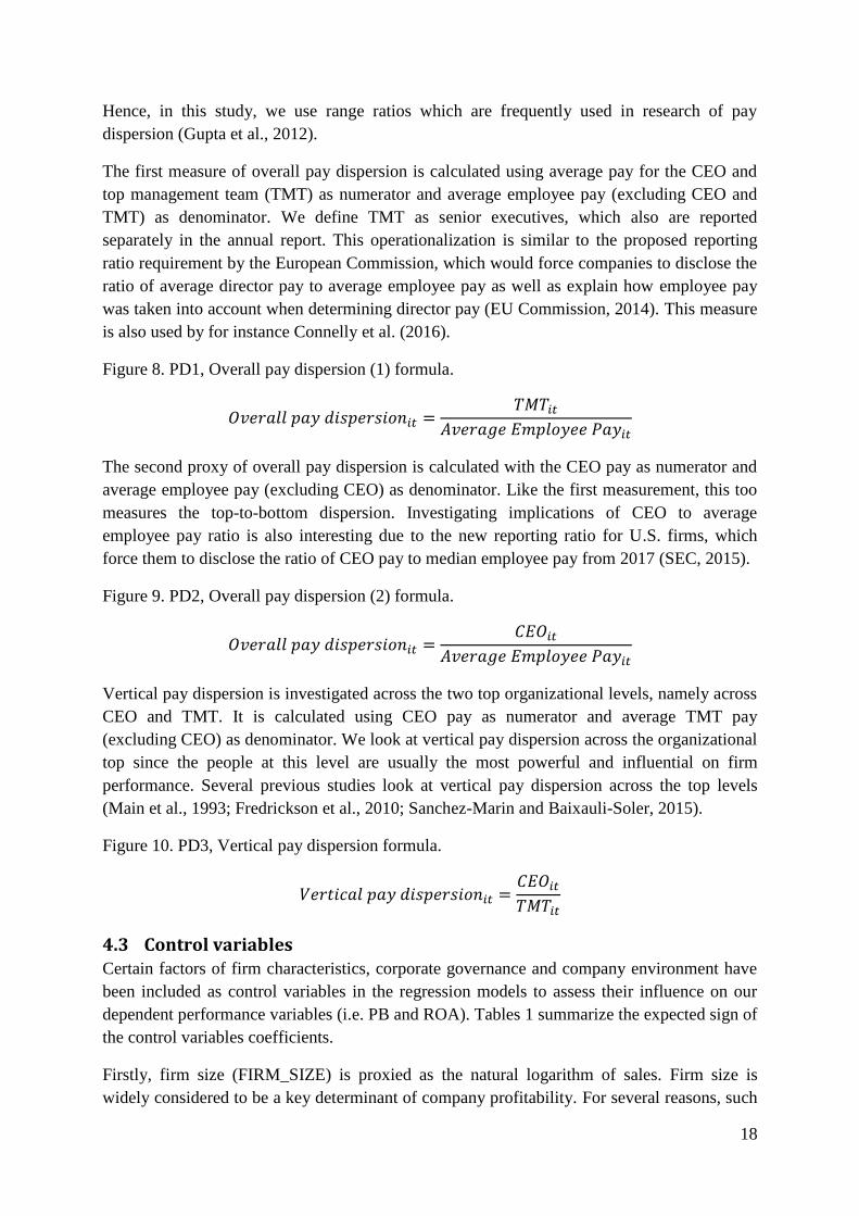
Hence, in this study, we use range ratios which are frequently used in research of pay

dispersion (Gupta et al., 2012).

The first measure of overall pay dispersion is calculated using average pay for the CEO and

top management team (TMT) as numerator and average employee pay (excluding CEO and

TMT) as denominator. We define TMT as senior executives, which also are reported

separately in the annual report. This operationalization is similar to the proposed reporting

ratio requirement by the European Commission, which would force companies to disclose the

ratio of average director pay to average employee pay as well as explain how employee pay

was taken into account when determining director pay (EU Commission, 2014). This measure

is also used by for instance Connelly et al. (2016).

Figure 8. PD1, Overall pay dispersion (1) formula.

𝑂𝑣𝑒𝑟𝑎𝑙𝑙 𝑝𝑎𝑦 𝑑𝑖𝑠𝑝𝑒𝑟𝑠𝑖𝑜𝑛𝑖𝑡 =𝑇𝑀𝑇𝑖𝑡

𝐴𝑣𝑒𝑟𝑎𝑔𝑒 𝐸𝑚𝑝𝑙𝑜𝑦𝑒𝑒 𝑃𝑎𝑦𝑖𝑡

The second proxy of overall pay dispersion is calculated with the CEO pay as numerator and

average employee pay (excluding CEO) as denominator. Like the first measurement, this too

measures the top-to-bottom dispersion. Investigating implications of CEO to average

employee pay ratio is also interesting due to the new reporting ratio for U.S. firms, which

force them to disclose the ratio of CEO pay to median employee pay from 2017 (SEC, 2015).

Figure 9. PD2, Overall pay dispersion (2) formula.

𝑂𝑣𝑒𝑟𝑎𝑙𝑙 𝑝𝑎𝑦 𝑑𝑖𝑠𝑝𝑒𝑟𝑠𝑖𝑜𝑛𝑖𝑡 =𝐶𝐸𝑂𝑖𝑡

𝐴𝑣𝑒𝑟𝑎𝑔𝑒 𝐸𝑚𝑝𝑙𝑜𝑦𝑒𝑒 𝑃𝑎𝑦𝑖𝑡

Vertical pay dispersion is investigated across the two top organizational levels, namely across

CEO and TMT. It is calculated using CEO pay as numerator and average TMT pay

(excluding CEO) as denominator. We look at vertical pay dispersion across the organizational

top since the people at this level are usually the most powerful and influential on firm

performance. Several previous studies look at vertical pay dispersion across the top levels

(Main et al., 1993; Fredrickson et al., 2010; Sanchez-Marin and Baixauli-Soler, 2015).

Figure 10. PD3, Vertical pay dispersion formula.

𝑉𝑒𝑟𝑡𝑖𝑐𝑎𝑙 𝑝𝑎𝑦 𝑑𝑖𝑠𝑝𝑒𝑟𝑠𝑖𝑜𝑛𝑖𝑡 =𝐶𝐸𝑂𝑖𝑡

𝑇𝑀𝑇𝑖𝑡

4.3 Control variables Certain factors of firm characteristics, corporate governance and company environment have

been included as control variables in the regression models to assess their influence on our

dependent performance variables (i.e. PB and ROA). Tables 1 summarize the expected sign of

the control variables coefficients.

Firstly, firm size (FIRM_SIZE) is proxied as the natural logarithm of sales. Firm size is

widely considered to be a key determinant of company profitability. For several reasons, such

19

as economies of scale and market power, larger firms are traditionally considered favored to

smaller firms in the same industry. (Lee, 2009) Because of this, several previous research of

pay dispersion includes firm size as a control variable that is expected to positively affect firm

performance (e.g. Lee et al., 2008; Sanchez-Marin and Baixauli-Soler, 2015; Siegel and

Hambrick, 2005; Grund and Westergaard-Nielsen, 2008; Heyman, 2005). How firm size is

measured differs from log of sales, to log of value of assets and number of employees. Since

we include companies from all industries, we measure firm size by natural log of sales since

both number of employees and value of assets differs vastly depending on which industry the

company belongs to.

Secondly, prior year performance is measured as ROA or PB for year T-1 (PRIOR_PERF).

According to Connelly et al. (2016), prior performance is generally a strong indicator for

future performance and thus should be included as a control variable.

Thirdly, to control for firm-specific effects of corporate governance mechanisms, the log of

number of board members (BOARD_SIZE) and a dummy for whether the CEO is a member

of the board (CEO_IN_BOARD) are also included.

Board size is measured as the log of number of board directors, as used by Yermack (1996),

Lee et al. (2008) and Guest (2009). The theory on board size suggests that smaller boards in

general experience greater effectiveness than larger boards (Jensen, 1993; Lipton and Lorsch,

1992). However, increasing the size initially of a very small board is positive for board

effectiveness as it facilitates the boards’ key functions (Jensen, 1993; Lipton and Lorsch,

1992). For instance, one vital board function, advising, is facilitated initially by the increase

in board size as the greater board has the advantage of a greater combined knowledge base

and expertise (Dalton et al., 1999; 2005). This initial positive effect is however offset by other

factors as the size increases.

There are two main reasons to why larger boards are less effective than smaller boards. First,

there is the disadvantage of coordination and communication costs (Jensen, 1993). There is an

inherent difficulty for larger boards to schedule meetings and reach consensus which leads to

slow and inefficient decision-making. Second, there is the issue of board members free-riding

(Jensen, 1993; Lipton and Lorsch, 1992). The increase in board size will decrease the cost and

incentive of each board member to, for example, monitor as thorough as before. Thus, larger

boards will have a greater problem of board directors free-riding.

Research on board size is rather uniform and confirms the theory of larger boards being less

effective and consequently having a negative effect on performance (Cheng et al., 2008;

Hermalin and Weisbach. 2003). For instance, Paul Guest (2009) using a sample of 2746 UK

listed firms examines the impact of board size on performance. His findings show a strong

negative and significant relationship between board size and three different measures of

performance (i.e. ROA, Tobin’s Q and share return). A similar negative relationship is found

using data from Scandinavian firms in the study by Conyon and Peck (1998).

20

A significant difference between boards in Swedish companies and companies from USA is

that CEOs are Sweden is prohibited by the Swedish Code of Corporate Governance to act as

chairman of the board, so called CEO duality (Randøy and Nielsen, 2002). According to Duru

et al., (2016) CEO duality and its effect on firm performance have been widely researched.

They describe how this research yields mixed results, thus supporting two different theoretical

perspectives. Firstly, agency theory argues for negative effects in firm performance since the

board independence becomes compromised, resulting in reduced control and influence over

the CEO. In contrast, stewardship theory and resource dependence theory argues that CEO

duality leads to increased corporate flexibility and effectiveness, which in turn have positive

effects on firm performance.

Despite the fact that CEOs in Swedish firms cannot be chairman of the board, it is not

uncommon that they are included in the board as board director. We argue that the effect on

firm performance of the CEO being a board member is similar to CEO duality.

Lastly, year dummy variables (YEAR_DUMMIES) are used to control for year-specific

effects, such as influential macro events, and aggregate time series trends, such as economic

growth, population growth and inflation (Stock and Watson, 2012).

Table 1. Predicted sign of coefficients

Variable Sign Description

Prior performance + Change in performance (ROA or PB), one years prior to the focal year of the analysis

Firm size + Change of natural log of sales

Board size - Change of number of board directors

CEO in board +/- Change of CEO as board director-dummy

PD Short term + Three different proxies are used for pay dispersion. To capture short, medium and long-term effects, the change of pay dispersion is measured one, two and three years prior to the focal year of the analysis.

PD Medium term +/-

PD Long term -

Table 1 display the predicted sign for each independent variable included in the regression model, as well as a short description of how each variable is measured. The predicted signs are based on theory and previous research. + predicts a positive coefficient, - predicts a negative coefficient. +/- are used when there is no expected direction of the variables effect on firm performance.

21

4.4 Data collection Our dataset includes all firms on the OMX Stockholm indexes for large-, mid- and small-cap

Swedish firms for the years 2010 and 2015. The inclusion of large, mid, and small-cap

companies in the sample provides a dataset covering all industries in the Swedish market. As

our regression model is designed, each observation requires data from four years prior to the

focal year. Data is therefore collected for the six-year period ranging from 2010 to 2015.

The data is collected from four sources. Pay data is retrieved manually from the firms’ annual

reports. Market capitalization as well as book value of equity is gathered from the Eikon

database. Other financial data is collected from Retriever Business database. Lastly, board

composition data is retrieved from the book Styrelser och Revisorer: i Sveriges Börsföretag

(Sundqvist et al., 2013; Sundqvist et al., 2014). Since no book from Sundqvist et al. has been

published for 2015, data on board composition for that year is collected from annual reports

using the same methodology as Sundqvist et al. The data is examined by drawing random

samples and checking outliers against the data in annual report. All variables, except the

dummies and board size, are winsorized at 5% to address the issue of outliers.

Furthermore, we find that Retriever Business at times incorrectly collects data from the parent

company instead of the entire group, which often results in extreme values. Because of this,

all the highest and lowest numbers for each variable are controlled and corrected up to a level

where errors no longer are found in the last five controlled.

We collect pay data on three levels; CEO pay, TMT pay and total pay for all employees. This

data, as well as the number of members in TMT and total number of employees which are

used to calculate average pay at each level, are all mandatory information to report in the

annual reports. Furthermore, according to the accounting standards, reported pay should

reflect fixed and variable salaries, value of paid out options during the year, other benefits and

pension. (ÅRL kap5. 40§) We use this annual report data of pay to calculate pay dispersion.

Our definition of pay therefore corresponds with the accounting principles described above.

Collecting pay dispersion data from annual reports differs from previous studies on pay

dispersion in Sweden. For instance, Heyman (2005) uses survey data while Hibbs and

Locking (2001) use wage data provided by three Swedish unions (LO, Metall and SAF). Data

from annual reports allows us to examine pay dispersion from an investor perspective. As

annual report data are publicly available and easily accessible for investors, a relationship

between pay dispersion and firm performance when using this data as source indicate an

opportunity to trade on this information.

In calculating Price to book, both market capitalization and book value of equity are collected

at the end of the fiscal year. Measuring PB at the end of the fiscal year constitutes a

measurement issue since the information of the annual report has not yet been disclosed to the

market. Consequently, market capitalization does not reflect the information from the annual

reports. A better approach would be to measure market capitalization at the release of the

annual report. However, due to limitations in time and the fact that all annual reports are

released at different dates, the data is instead retrieved at the end of the fiscal year.

22

4.5 Sample and descriptive statistics Our original sample consists of 269 firms (see Table 2) that were listed on small, mid or large

cap at 2014 or 2015. From this sample, financial firms are excluded because of their unique

characteristics. Furthermore, a number of companies are excluded due to lack of transparent

reporting regarding CEO pay, TMT pay and/or number of people in TMT. Additionally, due

to the fact that our model requires data from five consecutive years for each observation, 20

firms are deducted from the sample due to reasons that made them non applicable. For

different reasons, these firms either entered or left the stock market during the period 2010 -

2015. This inevitably introduces a degree of survival bias into the sample because of the fact

that only firms remaining listed during five consecutive years are included. However, this

effect is to a certain extent mitigated due to that the excluded observations are not as

mentioned solely bad performers. Furthermore, looking at all large- to small-cap Swedish

public firms also lowers the degree of survivor bias. This is related to taking account to firm’s

who both move up and down the indexes. Consequently, the sample comprises of 310

observations from 161 firms.

Table 2. Observations and sample size

Firms, initial sample 269

Financial firms -47

Pay-data not clearly disclosed -41

Missing long-term data -20

Firms, final sample 161

Number of firm-level observations 310 Table 2 shows the number of firms in the original sample, as well as exclusions of firms and number of observation used in the regression.

Table 3 shows descriptive statistics for our sample. Mean value for ROA is 2.7% and median

4.6%, suggesting that there are a few companies with very low ROA that lowers the mean

value. Furthermore, these relatively low numbers of ROA implies that the sample firms in

general are not very profitable. In contrast, the mean and median value for PB is 2.9 and 2.4

respectively. The mean value for firm size shows an average net sale of 10 342 MSEK. The

mean board size is 6.5 members and the CEO was in the board in 34.1% of all observations.

Jensen (1993) claim that the optimal board size is between seven or eight board directors,

whereas Lipton and Lorsch (1992) instead argue eight or nine is ideal. In our sample the mean

is 6.5 board members which is below their stated optimal levels.

The data also shows that a CEO in a firm listed on the OMX Stockholm indexes for large-,

mid- and small-cap, on average, received a yearly pay of 6.83 MSEK from 2010 to 2014. The

median value of the CEO pay was 4.33 MSEK, suggesting that there are CEO’s that receive

significantly more and drive up the mean value. Similarly, the mean top management pay

(excluding CEO) was during the period 2.5 MSEK and the median 1.9. Moreover, the average

TMT included 6 individuals. The three measures for pay dispersion displays a mean of 821%,

1765% and 252% respectively. It is reasonable that the second measure (PD2) displays the

largest mean since it measures the absolute top level (CEO) to average employee pay.

23

Likewise, it is reasonable that the third measure results in the lowest mean since it is the only

measure between two adjacent corporate levels (CEO to TMT). Furthermore, all pay

dispersion measures displays high interquartile ranges which suggests large variations of pay

dispersion within the sample.

Table 3. Descriptive statistics

Variable Mean Median Std. Dev IQ-Range 5% 95%

PB 2.946 2.376 2.151 2.505 0.506 8.657

ROA 0.027 0.046 0.103 0.074 -0.276 0.165

PD1 8.215 5.345 7.191 6.376 2.094 28.270

PD2 17.654 10.206 19.411 13.696 3.100 75.355

PD3 2.521 2.397 0.836 1.222 1.222 4.217

Firm size 10 342.230 1 665.285 20 973.790 6 104.965 66.101 83 888.000

log Firm size 7.552 7.418 1.935 2.599 4.191 11.337

Board size 6.463 6.000 1.497 2.000 4.000 9.000

log Board size 1.840 1.792 0.228 0.336 1.386 2.197

CEO in board1

0.341 0.000 0.474 1.000 0.000 1.000 1 CEO in board is a dummy taking value of 0 or 1

Table 3 displays the mean, the median, the standard deviation, the interquartile range, the 5th percentile and

the 95th percentile for each variable.

24

4.6 Correlation matrix

Table 4. Correlation matrix

Variable Prior PB Prior ROA PD1 S PD1 M PD1 L PD2 S PD2 M PD2 L PD3 S PD3 M PD3 L Firm size Board size CEO in board

Prior PB 1 Prior ROA -0.054 1

PD1 S -0.035 0.032 1 PD1 M -0.008 -0.021 -0.325*** 1

PD1 L 0.025 -0.004 0.001 -0.295*** 1 PD2 S -0.040 0.055 0.827*** -0.267*** 0.058 1

PD2 M 0.038 -0.031 -0.193*** 0.798*** -0.230*** -0.233*** 1 PD2 L 0.070 0.002 -0.076 -0.178*** 0.813*** -0.022 -0.204*** 1

PD3 S 0.017 0.039 -0.216*** 0.134*** 0.036 0.187*** -0.031 0.062 1 PD3 M 0.131*** 0.004 0.156*** -0.185*** 0.124** 0.046 0.243*** -0.023 -0.355*** 1

PD3 L 0.074 0.049 -0.155*** 0.096* -0.186*** -0.138** -0.020 0.237*** 0.031 -0.332*** 1 Firm size 0.060 0.009 0.010 -0.005 0.064 0.016 -0.005 0.069 0.031 0.034 0.042 1

Board size 0.068* 0.038 -0.002 -0.035 0.050 0.007 -0.019 0.015 0.016 -0.009 -0.029 0.062* 1 CEO in board 0.041* -0.020 0.059 0.012 0.036 0.005 0.010 0.072 -0.023 -0.020 -0.004 -0.027 0.103*** 1

Table 4 presents correlation between variables. Values above 0 denote positive correlation, values below 0 denote negative correlation. A value of +/- 1 represent perfect correlation and a value of 0 represent no correlation. ***, ** and * represent significance at the 1%, 5% and 10% levels respectively.

25

A correlation matrix is constructed (see Table 4 on previous page) to examine the existence of

possible multicollinearity problems. Correlations coefficients that exceeds +/- 0.8 indicate a

strong correlation and probable multicollinearity problem (Studenmund, 2014).

The relationships between PD1 and PD2 are the only ones that exhibit a severe correlation

(0.827 short, 0.798 medium, 0.813 long, all significant on the 1% level). This is not a

multicollinearity issue as PD1 and PD2 are two different proxies used in different regression

models. However, this indicates that the two proxies are statistically similar to each other and

to a large extent measure the same thing, which is not surprising as the only mathematical

difference between the two is that average TMT pay is moved from the numerator to the

denominator in PD2.

Other than that, the highest correlations are found in relationships within the pay dispersion

measures. For instance, PD3 short and PD3 medium have a correlation of -0.355 and PD3

medium and PD3 long have a correlation of -0.332, both significant at the 1% level. However,

we estimate that these correlations are too low to cause an issue of multicollinearity.

4.7 Determination of regression model Considering that our sample comprises of panel data, an OLS regression will increase the risk

of heteroscedasticity in the error terms and autocorrelation. With data characterized as such, a

fixed effect or random effects regression are used as better alternatives (Devers et al., 2008).

This is confirmed by a F-test conducted on our pooled OLS-regression, which result in

rejection (p < 0.00) of the null hypothesis, and therefore indicate a preference for random or

fixed effect models over pooled OLS.

Consequently, a Hausman test is conducted to test if the random-effects model is preferred

over the fixed effects model. The result of the Hausman test (p < 0.00) indicates that the fixed

effect regression is preferred over the random effects model. Thus, a fixed effects regression

model is used to test the hypotheses. Furthermore, we use robust standard errors to account

for disturbances of heteroscedasticity and autocorrelation existing in panel data.

26

5. Regression results The results from our regressions are presented in table 5 and 6 below. Price to book ratio is

used as dependent variable in table 5 and ROA is used as dependent variable in table 6. Each

table comprise of four models. Model 1 omits pay dispersion variables, whereas Model 2, 3

and 4 include different measures of pay dispersion. More specific, the second model tests the

first measure of pay dispersion (average pay for TMT including CEO to average employee

pay), the third model uses the second measure of pay dispersion (CEO pay to average

employee pay) and the fourth model tests the third measure for pay dispersion (CEO pay to

average TMT pay).

Table 5. Fixed Effects Panel Regression of Firm Performance Dependent variable: Price to book ratio

Variable Model 1.

No PD Model 2.

PD1 Model 3.

PD2 Model 4.

PD3

Constant -0.027

0.624 *** 0.613 *** 0.626 ***

(-0.37)

(6.93)

(6.99)

(6.54)

Prior perf (PB) -0.246 *** -0.477 *** -0.475 *** -0.527 ***

(-3.94)

(-3.12)

(-3.09)

(-3.57)

Firm size -0.093

-0.368

-0.310

-0.429

(-0.32)

(-0.59)

(-0.50)

(-0.65) Board size -0.006

-0.357

-0.309

-0.096

(-0.02)

(-0.51)

(-0.44)

(-0.13) CEO in board 0.055

0.277

0.346

0.392 *

(0.31)

(1.21)

(1.59)

(1.85)

Year dummies Included

Included

Included

Included

-

-

-

- PD Short term

0.005

0.011 ** 0.139

(0.45)

(2.37)

(1.31) PD Medium term

-0.033

0.002

0.521 ***

(-1.32)

(0.25)

(3.07) PD Long term

0.008

0.002

0.360 **

(0.46) (0.33) (2.25)

R2 within 0.139

0.334

0.327

0.365

Observations 655

310

310

310

Number of groups 179 161 161 161 Table 5 presents the results of the first difference fixed effects regression using PB as dependent variable. First row for each variable show beta coefficients and second row show t-values in parentheses. ***, ** and * represent significance at the 1%, 5% and 10% levels respectively. Model 1 include no measure of pay dispersion, Model 2 include PD1 as pay dispersion measure, Model 3 include PD2 as pay dispersion measure and Model 4 include PD3 as pay dispersion measure.

Table 5 shows the regression results with PB as dependent variable. It shows that Model 1,

which omits measure for pay dispersion, consists of 655 observations and has a R2

of 0.139.

When adding the first measure of pay dispersion in Model 2, R2 increases to 0.334 and the

sample size decreases to 310. Model 3 and Model 4 have the same sample size as Model 2

(310) and a R2 of 0.327 and 0.365 respectively.

27

Furthermore, the table displays that the coefficients for prior performance are negative and

significant at the 1% level in all four models. Board size show negative coefficients in Model

1, 2, 3 and 4 but none of them are significant. Likewise, firm size exhibits negative and

insignificant coefficients. In contrast, the CEO in board coefficients are positive in all four

models but only significant at the 10% level in Model 4.

The short-term measure of pay dispersion is positive in all three models. In the second and

third models, using PD1 and PD2 as measures respectively, the coefficients are 0.005 and

0.011. In the fourth model which uses PD3 as measure, the coefficient is 0.139. The short-

term pay dispersion variable is only significant in the model using PD2 as measure (at 5%).

The coefficients for medium term pay dispersion are negative for PD1 (-0.033), but positive

for PD2 (0.002) and PD3 (0.521). They are insignificant for PD1 and PD2, but significant at

the 1% level for PD3. Moreover, the long-term pay dispersion variable displays positive

coefficients for PD1 (0.008), PD2 (0.002) and PD3 (0.360). Significance at the 5% level is

found for the long-term variable using the PD3 measure. None of the other models have

significant coefficients for long-term pay dispersion.

Table 6. Fixed Effects Panel Regression of Firm Performance Dependent variable: Return on Assets

Variable Model 1.

No PD Model 2.

PD1 Model 3.

PD2 Model 4.

PD3

Constant -0.022 *** 0.008 * 0.008 * 0.009 *

(-4.02)

(1.96)

(1.93)

(1.89)

Prior perf (ROA) -0.454 *** -0.718 *** -0.718 *** -0.717 ***

(-7.25)

(-9.48)

(-9.49)

(-9.49)

Firm size 0.084 *** 0.111 *** 0.112 *** 0.114 ***

(3.18)

(3.21)

(3.22)

(3.30)

Board size -0.091 *** -0.056

-0.054

-0.049

(-3.81)

(-1.57)

(-1.57)

(-1.32) CEO in board -0.005

0.000

0.002

0.003

(-0.31)

(0.01)

(0.08)

(0.16) Year dummies Included

Included

Included

Included

-

-

-

- PD Short term

-0.001

-0.000

-0.001

(-0.91)

(-0.90)

(-0.15) PD Medium term

-0.002 * -0.000

0.000

(-1.69)

(-1.07)

(0.04) PD Long term

0.000

0.000

0.004 (0.12) (0.86) (0.57)

R2 within 0.337

0.652

0.650

0.649

Observations 653

309

309

309

Number of groups 179 161 161 161 Table 6 presents the results of the first difference fixed effects regression using ROA as dependent variable. First row for each variable show beta coefficients and second row show t-values in parentheses. ***, ** and * represent significance at the 1%, 5% and 10% levels respectively. Model 1 include no measure of pay dispersion, Model 2 include PD1 as pay dispersion measure, Model 3 include PD2 as pay dispersion measure and Model 4 include PD3 as pay dispersion measure.

28

Table 6 presents the fixed effects regression results with ROA as dependent variable. Model 1

has a R2 of 0.337 with 653 observations. Model 2, 3 and 4 all have a sample size of 309

observations. R2 is 0.652 in Model 2, 0.650 in Model 3 and 0.649 in Model 4.

The coefficients for prior performance are negative and significant at the 1% level in all four

models. The coefficients for board size are also negative in all models but only significant in

Model 1, which shows significance at the 1% level. The coefficient for CEO in board is

negative in Model 1 but positive in the following three. All are insignificant. Firm size is

positive and significant at the 1% level in all four models.

The coefficients for short-term pay dispersion are negative in all models. Medium-term pay

dispersion has a small and negative coefficient in Model 2 and Model 3, and a small and

positive coefficient in Model 4. The only significance found is in Model 2 at the 10% level.

For long-term pay dispersion, a small and insignificant positive coefficient is found in Model

2, 3 and 4.

5.1 Sensitivity analysis To check the robustness of the results, as well as the model specification, a sensitivity

analysis is conducted.

The fixed effects regression results show no clear indication of how and if pay dispersion

affect firm performance in the short and long-term. Furthermore, the significant result of the

PD3 long-term coefficient in Table 5 is contradictory to the expected. Thus, further testing is

necessary to conclude if these results are robust.

Apart from the pay dispersion variables, prior performance is of interest due to it showing a

consistent negative significant coefficient in all models which is opposite to the expected

theoretical sign. One explanation for this could be that the low sample size causes a spurious

negative relationship. Another likely explanation is omitted variable bias, as the coefficients

remain significant at the 1% level when testing different model specifications. However, an

entity and time fixed effects regression model, such as ours, control for unobserved omitted

variables that are constant over time or across entities (firms). Still, this model will not control

for unobserved omitted variables that are time variant and not constant across firms. Thus,

there could be a bias of an unobserved omitted variable that is time variant and not constant

across firms which would be a result of a specification bias. Lacking data on adequate control

variables that might be omitted makes it difficult to control for this potential effect. One

solution is to estimate an instrumental variable regression to mitigate this potential omitted

bias effect.

Thus, generalized method of moments (GMM), which is a type of instrumental variable

regression, is used to further check the robustness of our results and to control for the possible

omitted variable bias. GMM is also used to control for possible endogeneity in the regression

model. One possible endogeneity issue might be linked to board size and firm performance.

Research of board size show that board size is determined by firm-specific variables, such as

Tobin’s Q, ROA and firm size (Boone et al., 2007; Coles et al., 2008; Guest, 2008; Linck et

al., 2008). Furthermore, Wintoki et al. (2012) found indications that CEO board membership

29

might be dependent on previous firm performance and therefore endogenous. Endogeneity

between pay dispersion and firm performance have likely been mitigated by our usage of

lagged pay dispersion variables. Considering, the likely endogeneity problems it is reasonable

to use the GMM model to further check the robustness of our findings. The Sargan/Hansen

test of over-identifying restrictions will also be used to further control the accuracy of the

GMM and for the effects of endogeneity on the results.

Difference GMM is used, as it is suitable for panel data sets which are characterized by few

time periods (small T) and many firms (large N) (Roodman, 2009). Furthermore, instead of

first differences which increase data loss in unbalanced panels such as ours, we use the

Arellano and Bover estimator, i.e. forward orthogonal deviations (FOD) transformation.

According to Roodman (2009), lagged versions of the existing variables in the dataset

constitutes as good instruments. Thus, we use lags from 2 which are standard for endogenous

variables (Roodman, 2009), to 4 as further lags reduces our numbers of observations

significantly. All variables are lagged (except year dummies) according to this to ensure

exogeneity of instruments. To investigate if any effect of pay dispersion on firm performance

can be found at all, this GMM-approach will solely test if there is a general effect of pay

dispersion on performance without separating the long and short-time effects. Consequently,

this will render a larger sample size.

The results of the GMM are presented in Table 7 and Table 8 below. The Arellano and Bond

(AR(2)) test and Hansen p-values are >0.05 in all GMM-models, indicating no second-order

autocorrelation in the error term and that all instruments are determined to be exogenous

(Roodman, 2009).

In all models, prior performance is positively significant at the 1% with PB as dependent

variable (Table 7) and at the 5% level with ROA (Table 8). The positive direction is opposite

from the results of the fixed effects regressions which show negative coefficients. Hence, the

prior performance coefficients now show the expected sign. The change of direction indicates

that the theoretically unexpected negative sign in the fixed effects regression may have been

caused by a possible omitted variable bias. Moreover, it could also be due to the larger sample

used in the GMM in comparison to the fixed effects regressions.

Another contradictory result to the fixed effects regression is found in firm size. Firm size has

an unexpected negative, but insignificant, sign in the fixed effects model when using PB as

dependent variable. In contrast, the difference GMM output shows the expected positive sign

with significance at the 1% in two models and 10% in one model in Table 7. The larger

sample size and the GMM-approach which mitigates endogeneity and omitted variable issues

might be possible answers to why the direction and significance level is different. These

reasons might also help explain the difference in result of firm size in models using ROA as a

performance proxy. This variable shows positive and significant results in the fixed effects

models but positive and insignificant results in the difference GMM (see Table 8). Despite the

insignificant results in the GMM, there is still an indication of firm size having a positive

effect in the ROA models. In general, considering both the fixed effects and difference GMM-

results, firm size shows an indication of having a positive effect on ROA and PB. The

30

insignificant results of the two corporate governance variables Board size and CEO in board

are considered robust since both the fixed effects and GMM-results indicate no relationship.

Moreover, the GMM-results show positive but insignificant pay dispersion coefficients in all

models (see table 7 and 8). This indicates that the overall finding of no relationship in the

fixed effects regressions is considered robust.

Table 7. Difference GMM Regression of Firm Performance

Dependent variable: Price to book ratio

Variable Model 1.

PD1 Model 2.

PD2 Model 3.

PD3

Prior perf (PB) 0.668 *** 0.669 *** 0.640 ***

(3.18)

(2.88)

(2.78)

Firm size 2.049 * 2.664 *** 2.639 ***

(1.89)

(2.69)

(2.66)

Board size 1.400

0.993

0.630

(0.59)

(0.32)

(0.27)

CEO in board -0.018

0.138

0.046

(0.02)

(0.17)

(0.06)

Pay Dispersion 0.101

0.019

0.204 (0.65) (0.17) (0.47)

Year dummies Included Included Included

- - -

Arellano-Bond, AR (2) 0.104

0.086

0.115

Hansen 0.108

0.067

0.107

Number of instruments 19

19

19

Observations 655

655

655

Number of groups 179 179 179 Table 7 displays the results of the difference GMM regression using PB as dependent variable. First row for each variable show coefficients and second row show t-values in parentheses. ***, ** and * represent significance at the 1%, 5% and 10% levels respectively. Model 1 include PD1 as pay dispersion measure, Model 2 include PD2 as pay dispersion measure and Model 3 include PD3 as pay dispersion measure.

31

The results further indicate that prior performance is positively linked to firm performance.

This is in line with the theoretical assumption that historical performance is an indicator of

future performance (Connelly et al., 2016) as well as previous studies (Bloom and Michael,

2002). As for firm size, the results of our regressions also indicate a positive effect on firm

performance (both PB and ROA), once again in line with theory and other research (Lee,

2009, Heyman, 2005, Sanchez-Marin, 2015). This indicates that factors such as economies of

scale and market power do influence firm performance in the Swedish publicly listed

companies included in our sample. Our findings suggest that board size and CEO in board

have no effect on firm performance. Thus, the results of board size contradict the theory and

previous research which suggest a negative relationship to firm performance. However, as our

descriptive statistics show, the interquartile range is between 5 and 7 and the mean board size

of our sample is lower than the optimal level proposed by Lipton and Lorsch (1992) and

Jensen (1993). This can help explain why we do not find the same negative relationship as

previous studies. The theory of CEO in board is ambivalent to the effect on firm performance.

We use a slightly different definition of CEO in board compared to previous studies as there

are legal restrictions in Sweden that prohibit the CEO to act as chairman of the board. Our

insignificant result might be explained by the fact that, when a CEO cannot act as chairman,

her power and authority is mitigated.

Table 8. Difference GMM Regression of Firm Performance

Dependent variable: Return on Assets

Variable Model 1.

PD1 Model 2.

PD2 Model 3.

PD3

Prior perf (ROA) 0.288 ** 0.309 ** 0.314 **

(2.20)

(2.24)

(2.51)

Firm size 0.058

0.089

0.072

(0.92)

(1.21)

(1.51) Board size 0.195

0.297

0.133

(1.14)

(1.25)

(0.66) CEO in board 0.027

0.038

0.053

(0.71)

(0.91)

(1.31) Pay Dispersion 0.005

0.004

0.015

(0.94) (0.99) (0.74)

Year dummies Included Included Included

- - -

Arellano-Bond, AR (2) 0.154

0.182

0.125 Hansen 0.362

0.325

0.306

Number of instruments 19

19

19 Observations 653

653

653

Number of groups 179 179 179 Table 8 displays the results of the difference GMM regression using ROA as dependent variable. First row for each variable show coefficients and second row show t-values in parentheses. ***, ** and * represent significance at the 1%, 5% and 10% levels respectively. Model 1 include PD1 as pay dispersion measure, Model 2 include PD2 as pay dispersion measure and Model 3 include PD3 as pay dispersion measure.

32

To further robustness test the results and see if certain sample characteristics can influence the

results, a dummy of the size of pay dispersion (PD size dummy) is included and tested in

another GMM regression (see Appendix 2). This dummy takes a value of 1 if pay dispersion

is higher than the sample median and 0 if it is lower. By including this dummy, the regression

tests if the size of pay dispersion affects company performance, by splitting the sample into

two categories (i.e. high and low pay dispersion). Table 12 and 13 in Appendix 2 show no

significant result for the PD size dummy and the results for the pay dispersion variables also

remain insignificant.

33

6. Analysis and discussion Our first hypothesis states that pay dispersion positively affects firm’s short-term

performance. The results of our fixed effects regression show no significant effect of pay

dispersion on short-term firm performance, except in one of six models. This model use PB as

dependent variable and the second overall pay dispersion proxy; which measure top-to-

bottom pay dispersion as CEO pay to average employee pay. The relationship is positive and

significant at the 5% level, however the coefficient in this model, as well as all others, are

close to zero. This also indicates no effect. Regardless of performance measure and pay

dispersion proxy, further robustness tests using the difference GMM-approach, also provide

evidence of no significant short-term effects on performance. In regard to these findings of no

stable and consistent significant results, we reject Hypothesis 1 for all measures of pay

dispersion.

The second hypothesis states that pay dispersion negatively affects firm’s long-term

performance. Similar to the short-term findings, long-term effects of pay dispersion only

show significance in one of six fixed effects models. Here, Model 4 which uses PB as

dependent variable and the vertical pay dispersion between the CEO and TMT, results in a

significant coefficient at the 5% level. Furthermore, in this model, the effect of medium-term

pay dispersion is significant at the 1% level. These findings suggest that there is a positive

lagged time effect of vertical pay dispersion on firm performance. Interestingly, the

coefficients display positive relationships which contradict the expected negative association.

However, once again the sensitivity analysis using the difference GMM-approach reveals that

the results are not robust. For example, in GMM no significance is found for either pay

dispersions variable. Therefore, Hypothesis 2 is rejected for all measures of pay dispersion.

One explanation of why no short or long-term effects are found could be because there is

simply no effect of pay dispersion on firm performance at all. This is supported by our

findings. Our result of no effect of pay dispersion on firm performance lends no support for

tournament theory or the fairness approaches and contrasts the majority of previous research

that either finds a positive or negative relationship. However, in light of the ambivalent results

in research, the possibility of insignificant results is not surprising. Our findings are in line

with previous studies of vertical and overall pay dispersion by Leonard (1990) and Conyon et

al. (2001) that also finds no effect on firm performance. A vital distinction between these

previous studies and ours is the analysis of both long and short-term effects and the

geographical area of analysis.

Connelly et al. (2016) is the one study that focuses on both short and long-term effects of pay

dispersion on performance and uses a similar methodical approach. Their findings, opposite to

ours, suggest a positive short-term effect of higher pay dispersion and a negative long-term

effect of high pay dispersion. This difference in result might be explained in the differences in

sample. Connelly et al. (2016) extract their data from the firms listed on the S&P 1500 which

consists of U.S. firms. There are large dissimilarities between the U.S. and Swedish labor

markets such as the degree of wage-setting institutions (e.g. unions) and distribution of wages

that might help explain the difference in results. In Sweden, income taxes and cash benefits

are a vital part of redistributing income and consequently reducing pay dispersion in the

34

Swedish population (OECD 2015). In addition, Sweden has a history of strong wage-setting

institutions in the form of unions which have also been instrumental in keeping the minimum

wages high and overall pay dispersion levels low (Heyman, 2005). Consequently, this has

resulted in low pay dispersion in Sweden and lower pay dispersion than countries such as the

U.S. and other OECD countries (OECD, 2016). This is confirmed by comparing the

descriptive statistics in Connelly et al. (2016) study with ours. Their mean of pay dispersion,

measured as average TMT pay to average employee pay (i.e. our PD1), amounts to 49.45.

This is significantly larger than our PD1 mean of 8.22 Also, our value at the 95th percentile

(28.27) is lower than their mean. The large difference in pay dispersion might be a reason for

why different results are found. If this is the case, the insignificant results of this study may

indicate that there is no effect of pay dispersion on the performance of Swedish firms because

pay dispersion, in general, simply is too low.

This low pay dispersion might suggest that Swedish workers are rather contempt about their

salary in comparison to that of their supervisors as the wage difference is rather low. In other

words, the workers might think that the supervisors’ pay are fair and will not reduce their

effort even though there are pay differences. Thus, the low pay dispersion in Sweden might

render the fairness theories inapplicable in a Swedish setting. Furthermore, a similar argument

can be made to tournament theory. One can argue that overall low pay dispersion in Swedish

firms might not incentivize the workers to exert extra effort to advance into a higher position

with higher pay as the tournament prize (higher pay) is not large enough in comparison to

their present pay level (Audas et al., 2004; Lazear and Rosen, 1981; Connelly et al., 2014).

Thus, these facts and arguments could help explain why no robust positive or negative

significant results are found in our thesis.

However, the continuing trend of higher and higher pay dispersion in Sweden (OECD 2015)

might suggest that tournament and fairness theories will be more applicable in the future as

the pay dispersion increases in Sweden. To our knowledge, the question of what level of pay

dispersion is needed to spur the effects of tournament theory or fairness approaches have not

been thoroughly investigated.

In contrast to these arguments for why pay dispersion may have limited effect on performance

in Swedish firms, are the previous studies of Hibbs and Locking (2001) and Heyman (2005)

that find positive and significant effects. The reasons for why they find positive results when

we do not, could perhaps be explained by methodical differences. For example, Hibbs and

Locking’s (2001) approach differs vastly from ours as they focus on pay dispersion within

industrial plants and their study do not account for issues of endogeneity.

Heyman (2005) finds, in his study of Swedish firms, a positive and significant effect of

overall pay dispersion on performance. Despite the lack of robust significant results in our

paper, the GMM-results, indicate by the positive yet insignificant coefficients for the overall

pay dispersion measures that a positive relationship might exist. However, there are multiple

important differences in the methodology used that could help explain the different findings.

For example, while our dataset is based upon aggregated firm data, Heyman (2005) to a larger

extent uses detailed pay data on an individual level. In addition, the sample in this thesis

35

comprises of only publicly listed firms on OMX Stockholm while Heyman’s sample does not

have this restriction and consequently includes a wider variety of Swedish firms. Thus,

Heymans (2005) sample might include a bigger proportion of smaller firms, in terms of

number of workers, characterized by certain attributes and perhaps having organizational

differences to the firms in our sample. The differences in results could perhaps also be

attributed to the differences in sample size. While Heyman’s sample comprises of 5800

observations ours consists of only 310 observations. The low sample size is a weakness of this

paper and a larger sample would perhaps result in different findings.

36

7. Conclusion The aim of this thesis is to examine if pay dispersion affect performance in publicly traded

Swedish companies. No effect of pay dispersion on firm performance is found neither on

short nor on long-term. Therefore, we conclude that there is no effect of pay dispersion on

firm performance in companies listed on OMX Stockholm’s index for small, mid or large cap.

In the study, two measures of overall pay dispersion and one measure of vertical pay

dispersion are included. In addition, two distinctly different measurements of firm

performances (PB and ROA) are applied. The conclusion applies to both overall and vertical

pay dispersion, regardless of performance metric.

As outlined in the discussion, two main reasons can explain this conclusion. Firstly, pay

dispersion in Sweden may simply be too low for tournament theory and the fairness

approaches to be applicable. Secondly, an alternative is that differences in method and

foremost smaller sample size might explain why our results differ from other Swedish studies.

This paper deepens and renews the knowledge of pay dispersion in Sweden, thus contributing

to existing literature. Research of both short and long-term effects of pay dispersion is limited

and therefore this thesis brings insight to this matter in a Swedish context. These time-effects

of pay dispersion could be further developed and researched using a larger sample.

Being the first Swedish paper that gathers data from annual reports to calculate pay

dispersion, this thesis also contributes to research of pay dispersion as a means of

performance indicator for investor to trade on. This aspect is interesting as the newly

implemented requirements in the U.S. and proposed requirements in EU-legislation, of

disclosing pay dispersion ratios in financial reports, makes the pay dispersion information

more accessible. However, the insignificant results suggest that investors would not be able to

trade on this new information in Sweden.

Still, the U.S. and EU reporting requirements might have implications that are of interest for

future research. A transparent reporting of pay dispersion might increase the public awareness

to the large dispersion in pay within firms. The risk of receiving negative publicity (hurting

brand value) from having high dispersion may put pressure on firm to take actions for lower

pay dispersion. This could possibly be investigated as an event study measuring effects before

and after the implementation of the disclosure requirements.

37

8. References Adams, J.S., 1965. Inequity In Social Exchange, in: Advances in Experimental Social

Psychology. Elsevier, pp. 267–299.

Adams, J.S., 1963. Towards an Understanding of Inequity. J. Abnorm. Soc. Psychol. 67, pp.

422–436.

Akerlof, G.A., Yellen, J.L., 1990. The Fair Wage-Effort Hypothesis and Unemployment. Q. J.

Econ. 105, pp. 255-283.

Audas, R., Barmby, T., Treble, J., 2004. Luck, Effort, and Reward in an Organizational

Hierarchy. J. Labor Econ. 22, pp. 379–395.

Backes-Gellner, U., Pull, K., 2013. Tournament Compensation Systems, Employee

Heterogeneity, and Firm Performance. Hum. Resour. Manage. 52, pp. 375–398.

Becker, B.E., Huselid, M.A., 1992. The Incentive Effects of Tournament Compensation

Systems. Adm. Sci. Q. 37, pp. 336-350.

Berri, D.J., Jewell, R.T., 2004. Wage inequality and firm performance: Professional

basketball’s natural experiment. Atl. Econ. J. 32, pp. 130–139.

Bloom, M., 1999. The Performance Effects of Pay Dispersion on Individuals and

Organizations. Acad. Manage. J. 42, pp. 25–40.

Boone, A.L., Casares Field, L., Karpoff, J.M., Raheja, C.G., 2007. The Determinants of

Corporate Board Size and Composition: An Empirical Analysis. J. Financ. Econ. 85,

pp. 66–101.

Borghesi, R., 2008. Allocation of Scarce Resources: Insight from the Nfl Salary Cap. J. Econ.

Bus. 60, pp. 536–550.

Bornschier, V., Ballmer-Cao, T.-H., 1979. Income Inequality: A Cross-National Study of the

Relationships Between MNC- Penetration, Dimensions of the Power Structure and

Income Distribution. Am. Sociol. Rev. 44, pp. 487-506.

Bothner, M.S., Kang, J., Stuart, T.E., 2007. Competitive Crowding and Risk Taking in a

Tournament: Evidence from NASCAR Racing. Adm. Sci. Q. 52, pp. 208–247.

Boyle, E., Shapira, Z., 2012. The Liability of Leading: Battling Aspiration and Survival Goals

in the Jeopardy! Tournament of Champions. Organ. Sci. 23, pp. 1100–1113.

Brealey, R.A., Myers, S.C., 1991. Principles of Corporate Finance, 4th ed. ed, McGraw-Hill

series in finance. McGraw-Hill, New York.

Carrell, M.R., Dittrich, J.E., 1978. Equity Theory: The Recent Literature, Methodological

Considerations, and New Directions. Acad. Manag. Acad. Manag. Rev. 3, 202.

Chen, J., Shum, M., 2010. Estimating a tournament model of intra-firm wage differentials. J.

Econom. 155, pp. 39–55.

Cheng, S., Evans III, J.H., Nagarajan, N.J., 2008. Board Size and Firm Performance: The

Moderating Effects of the Market for Corporate Control. Rev. Quant. Finance

Account. 31, pp. 121–145.

Coles, J.L., Naveen, L., Daniel, N.D., 2008. Boards: Does one size fit all? J. Financ. Econ. 87,

pp. 329–356.

Connelly, B.L., Haynes, K.T., Tihanyi, L., Gamache, D.L., Devers, C.E., 2016. Minding the

Gap: Antecedents and Consequences of Top Management-To-Worker Pay Dispersion.

J. Manag. 42, pp. 862–885.

Connelly, B.L., Tihanyi, L., Crook, T.R., Gangloff, K.A., 2014. Tournament Theory: Thirty

Years of Contests and Competitions. J. Manag. 40, pp. 16–47.

Conyon, M.J., Peck, S., 1998. Board size and corporate performance: evidence from

European countries. Eur. J. Finance 4, pp. 291–304.

Conyon, M.J., Peck, S.I., Sadler, G.V., 2001. Corporate Tournaments and Executive

Compensation: Evidence from the U.K. Strateg. Manag. J. 22, pp. 805–815.

38

Cowherd, D.M., Levine, D.I., 1992. Product Quality and Pay Equity Between Lower-Level

Employees and Top Management: An Investigation of Distributive Justice Theory.

Adm. Sci. Q. 37, pp. 302–320.

Dallas, L.L., 2012. Short-Termism, the Financial Crisis, and Corporate Governance. J. Corp.

Law 37, pp. 265-364.

Dalton, C.M., Dalton, D.R., 2005. Boards of Directors: Utilizing Empirical Evidence in

Developing Practical Prescriptions. Br. J. Manag. 16, pp. 91–97.

Dalton, D.R., Daily, C.M., Johnson, J.L., Ellstrand, A.E., 1999. Number of Directors and

Financial Performance: A Meta-Analysis. Acad. Manage. J. 42, pp. 674–686.

Debrock, L., Hendricks, W., Koenker, R., 2004. Pay and Performance: The Impact of Salary

Distribution on Firm-Level Outcomes in Baseball. J. Sports Econ. 5, pp. 243–261.

Depken, C.A., 2000. Wage Disparity and Team Productivity: Evidence from Major League

Baseball. Econ. Lett. 67, pp. 87–92.

Dole, C., 2015. Wage Dispersion’s Effectacross Team Units: Evidence from the National

Football League. J. Econ. Econ. Educ. Res. Arden 16, pp. 53–65.

Ehrenberg, R.G., Bognanno, M.L., 1990. The Incentive Effects of Tournaments Revisited:

Evidence from the European Pga Tour. Ind. Labor Relat. Rev. 43, pp. 74–88.

Eriksson, T., 1999. Executive Compensation and Tournament Theory: Empirical Tests on

Danish Data. J. Labor Econ. 17, pp. 262–280.

European Commision, 2014. Directive of the European Parliament and of the Council

Amending Directive 2007/36/Ec as Regards the Encouragement of Long-Term

Shareholder Engagement and Directive 2013/34/Eu as Regards Certain Elements of

the Corporate Governance Statement.

Fredrickson, J.W., Davis-Blake, A., Sanders, W.G., 2010. Sharing the Wealth: Social

Comparisons and Pay Dispersion in the CEO’s Top Team. Strateg. Manag. J. 31, pp.

1031–1053.

Frick, B., 2003. Contest theory and sport. Oxf. Rev. Econ. Policy 19, pp. 512-529.

Fristedt, D., Larsson, Å., Sundqvist, S.-I., 2014. Styrelser och revisorer i Sveriges börsföretag.

2014-2015. SIS Ägarservice, Stockholm.

Fristedt, D., Larsson, Å., Sundqvist, S.-I., 2013. Styrelser och revisorer i Sveriges börsföretag.

2013-2014. SIS Ägarservice, Stockholm.

Fristedt, D., Larsson, Å., Sundqvist, S.-I., 2012. Styrelser och revisorer i Sveriges börsföretag.

2012-2013. SIS Ägarservice, Stockholm.

Fristedt, D., Larsson, Å., Sundqvist, S.-I., 2011. Styrelser och revisorer i Sveriges börsföretag.

2011-2012. SIS Ägarservice, Stockholm.

Fristedt, D., Larsson, Å., Sundqvist, S.-I., 2010. Styrelser och revisorer i Sveriges börsföretag.

2010-2011. SIS Ägarservice, Stockholm.

Gillis, W.E., McEwan, E., Crook, T.R., Michael, S.C., 2011. Using Tournaments to Reduce

Agency Problems: The Case of Franchising. Entrep. Theory Pract. 35, pp. 427-447.

Greckhamer, T., 2016. CEO compensation in relation to worker compensation across

countries: The configurational impact of country-level institutions. Strateg. Manag. J.

37, pp. 793-815.

Grund, C., Westergaard-Nielsen, N., 2008. The Dispersion of Employees’ Wage Increases

and Firm Performance. Ind. Labor Relat. Rev. 61, pp. 485–501.

Guest, P., 2009. The impact of board size on firm performance: evidence from the UK. Eur. J.

Finance 15, pp. 385–404.

Guest, P.M., 2008. The determinants of board size and composition: Evidence from the UK.

J. Corp. Finance 14, pp. 51–72.

Gupta, N., Conroy, S.A., Delery, J.E., 2012. The Many Faces of Pay Variation. Hum. Resour.

Manag. Rev. 22, pp. 100–115.

39

Hayes, R.H., Abernathy, W.J., 1980. Managing Our Way to Economic Decline. Harv. Bus.

Rev. 58, pp. 67-77.

Henderson, A.D., Fredrickson, J.W., 2001. Top Management Team Coordination Needs and

the Ceo Pay Gap: A Competitive Test of Economic and Behavioral Views. Acad.

Manage. J. 44, pp. 96–117.

Hermalin, B.E., Weisbach, M.S., 2003. Boards of Directors as an Endogenously Determined

Institution: A Survey of the Economic Literature. Econ. Policy Rev. - Fed. Reserve

Bank N. Y. 9, pp. 7.

Heyman, F., 2005. Pay Inequality and Firm Performance: Evidence from Matched Employer-

Employee Data. Appl. Econ. 37, pp. 1313–1327.

Hibbs, D.A.J., Locking, H., 2000. Wage dispersion and productive efficiency: Evidence for

Sweden. J. Labor Econ. 18, pp. 755-782.

Hofstede, G., 2001. Culture’s Consequences: Comparing Values, Behaviors, Institutions, and

Organizations Across Nations, 2. ed., [Nachdr.]. ed. Sage Publ, Thousand Oaks, Calif.

Hofstede, G., Hofstede, G.J., Minkov, M., 2010. Cultures and Organizations: Software of the

Mind. McGraw-Hill.

Jensen, M.C., 1993. The Modern Industrial Revolution, Exit, and the Failure of Internal

Control Systems. J. Finance 48, pp. 831–880.

Kalra, A., Shi, M., 2001. Designing Optimal Sales Contests: A Theoretical Perspective. Mark.

Sci. 20, pp. 170–193.

Kessler, E.H. (Ed.), 2013. Encyclopedia of management theory. SAGE Publications, Inc,

Thousand Oaks, California.

Kidwell, R.E., Nygaard, A., 2011. A Strategic Deviance Perspective on the Franchise Form of

Organizing. Entrep. Theory Pract. 35, pp. 467–482.

Knoeber, C.R., 1989. A Real Game of Chicken: Contracts, Tournaments, and the Production

of Broilers. J. Law Econ. Organ. 5, pp. 271-292.

Knoeber, C.R., Thurman, W.N., 1994. Testing the theory of tournaments: an empirical

analysis of broiler production. J. Labor Econ. 12, pp. 155-179.

Lambert, R.A., Larcker, D.F., Weigelt, K., 1993. The structure of organizational incentives.

Adm. Sci. Q. 38, pp. 438-461.

Laverty, K.J., 2004. Managerial myopia or systemic short-termism? Manag. Decis. 42, pp.

949–962.

Laverty, K.J., 1996. Economic “Short-Termism”: The Debate, the Unresolved Issues, and the

Implications for Management Practice and Research. Acad. Manage. Rev. 21, pp.

825–860.

Lazear, E.P., 1999. Personnel Economics: Past Lessons and Future Directions. J. Labor Econ.

17, pp. 199-236.

Lazear, E.P., 1998. Personnel Economics for Managers. Wiley, New York.

Lazear, E.P., 1989. Pay Equality and Industrial Politics. J. Polit. Econ. 97, pp. 561–580.

Lazear, E.P., Rosen, S., 1981. Rank-Order Tournaments as Optimum Labor Contracts. J.

Polit. Econ. 89, pp. 841–864.

Lee, J., 2009. Does Size Matter in Firm Performance? Evidence from US Public Firms. Int. J.

Econ. Bus. 16, pp. 189-203.

Lee, K.W., Lev, B., Yeo, G.H.H., 2008. Executive pay dispersion, corporate governance, and

firm performance. Rev. Quant. Finance Account. 30, pp. 315–338.

Leonard, J.S., 1990. Executive Pay and Firm Performance. Ind. Labor Relat. Rev. 43, pp. 13–

29.

Levine, D.I., 1991. Cohesiveness, productivity, and wage dispersion. J. Econ. Behav. Organ.

15, pp. 237–255.

40

Linck, J.S., Netter, J.M., Yang, T., 2008. The determinants of board structure. J. Financ.

Econ. 87, pp. 308–328.

Lipton, M., Lorsch, J.W., 1992. A Modest Proposal for Improved Corporate Governance.

Bus. Lawyer 48, pp. 59–77.

Main, B.G.M., Reilly, C.A.O., Wade, J., 1993. Top Executive Pay: Tournament or

Teamwork? J. Labor Econ. 11, pp. 606-628.

Marginson, D., McAulay, L., 2008. Exploring the Debate on Short-Termism: A Theoretical

and Empirical Analysis. Strateg. Manag. J. 29, pp. 273-292.

Martin, J., 1981. Relative Deprivation: A Theory of Distributive Injustice for an Era of

Shrinking Resources, in: In L.L Cummings & B.M. Staws (Eds.), Research in

Organizational Behavior. CT: JAI Press, Greenwich, pp. 53–107.

Martins, P.S., 2008. Dispersion in Wage Premiums and Firm Performance. Econ. Lett. 101,

pp. 63–65.

McLaughlin, K.J., 1988. Aspects of tournament models: A survey. Res. Labor Econ. 9, pp.

225–256.

Milgrom, P., Roberts, J., 1990. The Efficiency of Equity in Organizational Decision

Processes. Am. Econ. Rev. 80, pp. 154–159.

Milgrom, P.R., 1988. Employment Contracts, Influence Activities, and Efficient Organization

Design. J. Polit. Econ. 96, pp. 42–60.

Milkovich, G.T., Newman, J.M., Gerhart, B.A., 2011. Compensation, 10th ed. ed. McGraw-

Hill Irwin, New York.

Mondello, M., Maxcy, J., 2009. The impact of salary dispersion and performance bonuses in

NFL organizations. Manag. Decis. 47, pp. 110–123.

Munck, J., 2016. Sveriges Rikes Lag: gillad och antagen på Riksdagen år 1734, stadfäst av

Konungen den 23 januari 1736 : med tillägg innehållande författningar som utkommit

från trycket fram till början av januari 2016. Wolters Kluwer, Stockholm.

Nafziger, E.W., Nafziger, E.W., 2006. Economic development, 4th ed. ed. Cambridge

University Press, Cambridge ; New York.

Nalebuff, B.J., Stiglitz, J.E., 1983. Prizes and Incentives: Towards a General Theory of

Compensation and Competition. Bell J. Econ. 14, pp. 21–43.

Nandorf, T., 2017. LO: Direktörer tjänar 54 gånger mer än sina arbetare [WWW Document].

DN.SE. URL http://www.dn.se/ekonomi/lo-direktorer-tjanar-54-ganger-mer-an-sina-

arbetare/ (accessed 5.12.17).

Narayanan, M.P., 1985. Observability and the Payback Criterion. J. Bus. 58, 309.

Nordström, J., 2016. Börsens bäst betalda: Håvar in 295 miljoner [WWW Document].

SvD.se. URL https://www.svd.se/borsens-bast-betalda-havar-in-295-miljoner

(accessed 5.12.17).

OECD, 2016. OECD Employment Outlook 2016. OECD Publishing Paris.

OECD, 2015. OECD Income inequality data update: Sweden (January 2015). OECD

Publishing Paris.

OECD, n.d. Social Expenditure Database (SOCX) [WWW Document]. OECD. URL

http://www.oecd.org/social/expenditure.htm (accessed 3.10.17a).

OECD, n.d. OECD Income Distribution Database [WWW Document]. OECD. URL

http://stats.oecd.org/Index.aspx?DataSetCode=IDD (accessed 3.24.17b).

Orszag, J.M., 1994. A New Look at Incentive Effects and Golf Tournaments. Econ. Lett. 46,

pp. 77–88.

Penman, S.H., 2013. Financial Statement Analysis and Security Valuation. McGraw-Hill

Higher Education.

41

Poujol, F.J., Tanner, J.F., 2010. The Impact of Contests on Salespeople’s Customer

Orientation: An Application of Tournament Theory. J. Pers. Sell. Sales Manag. 30, pp.

33-46.

Price, B.M., 2003. How Green Was My Valley? An Examination of Tournament Theory as a

Governance Mechanism in Silicon Valley Law Firms. Law Soc. Rev. 37, pp. 731-764.

Pritchard, R.D., 1969. Equity theory: A review and critique. Organ. Behav. Hum. Perform. 4,

pp. 176–211.

Ramaswamy, R., Rowthorn, R.E., 1991. Efficiency Wages and Wage Dispersion. Economica

58, pp. 501-514.

Randoy, T., Nielsen, J., 2002. Company Performance, Corporate Governance, and CEO

Compensation in Norway and Sweden. J. Manag. Gov. 6, pp. 57-81.

Rappaport, A., 2005. The Economics of Short-Term Performance Obsession. Financ. Anal. J.

61, pp. 65–79.

Roodman, D., 2009. How to do xtabond2: An introduction to difference and system GMM in

Stata. Stata J. 9, pp. 86–136.

Rosen, S., 1986. Prizes and incentives in elimination tournaments. Am. Econ. Rev. 76, pp.

701-715.

Sanchez-Marin, G., Baixauli-Soler, J.S., 2015. TMT pay dispersion and firm performance: the

moderating role of organizational governance effectiveness. J. Manag. Organ. 21, pp.

436–459.

SEC, 2015. Pay Ratio Disclosure 17 CFR Parts 229 and 249.

SFS 2015:813. Årsredovisningslag (1995:1554).

Shaw, J.D., 2014. Pay Dispersion. Annu. Rev. Organ. Psychol. Organ. Behav. 1, pp. 521–544.

Shaw, J.D., Gupta, N., Delery, J.E., 2002. Pay Dispersion and Workforce Performance:

Moderating Effects of Incentives and Interdependence. Strateg. Manag. J. 23, pp. 491–

512.

Siegel, P.A., Hambrick, D.C., 2005. Pay Disparities Within Top Management Groups:

Evidence of Harmful Effects on Performance of High-Technology Firms. Organ. Sci.

16, pp. 259–274.

Solomon, E., Laya, J.C., 1967. Measurement of company profitability : some systematic

errors in the accounting rate of return. Financ. Res. Manag. Decis., Financial research

and management decisions. - New York [u.a.] : Wiley. - 1967, pp. 152-183.

Sommers, P., 1998. Work incentives and salary distributions in the national hockey league.

Atl. Econ. J. 26, pp.119-119.

Statistiska Centralbyrån, 2017. Total income from employment and business 2000 and 2013–

2015, by municipality. Median in 2015 prices [WWW Document]. Stat. Cent. URL

http://www.scb.se/en/finding-statistics/statistics-by-subject-area/household-

finances/income-and-income-distribution/income-and-tax-statistics/pong/tables-and-

graphs/income--persons-counties-and-municipalities/total-income-from-employment-

and-business-preliminary-by-municipality-median/ (accessed 5.12.17).

Stock, J.H., Watson, M.W., 2012. Introduction to Econometrics, 3. ed., internat. global ed. ed,

The Pearson series in economics. Pearson, Boston, Mass.

Studenmund, A.H., 2014. Using Econometrics: A Practical Guide, Sixth edition, Pearson new

international edition. ed, Pearson custom library. Pearson Education, Harlow.

Swedish National Mediation Office, 2017. Den svenska arbetsmarknadsmodellen [WWW

Document]. Medlingsinstitutet. URL http://www.mi.se/kollektivavtal-lagar/den-

svenska-arbetsmarknadsmodellen/ (accessed 5.12.17).

The Economist, 2012. The new model. The Economist.

UNDP (Ed.), 2015. Work for human development, Human development report. United

Nations Development Programme, New York, NY.

42

Weigelt, K., Dukerich, J., Schotter, A., 1989. Reactions to Discrimination in an Incentive Pay

Compensation Scheme: A Game-Theoretic Approach. Organ. Behav. Hum. Decis.

Process. 44, pp. 26–44.

Wintoki, M.B., Linck, J.S., Netter, J.M., 2012. Endogeneity and the Dynamics of Internal

Corporate Governance. J. Financ. Econ. 105, pp. 581-606

Yermack, D., 1996. Higher market valuation of companies with a small board of directors. J.

Financ. Econ. 40, pp. 185–211.

43

9. Appendix

9.1 Appendix 1

Table 9. Correlations of lagged PD1

PD1 (t-1) PD1 (t-2) PD1 (t-3)

PD1 (t-1) 1 PD1 (t-2) 0.8999*** 1

PD1 (t-3) 0.8762*** 0.9216*** 1 The table shows a correlation matrix of different lags of the first measure of pay dispersion. Values above 0 denote positive correlation, values below 0 denote negative correlation. A value of +/- 1 represent perfect correlation and a value of 0 represent no correlation. ***, ** and * represent significance at the 1%, 5% and 10% levels

respectively.

Table 10. Correlations of lagged PD2

PD2 (t-1) PD2 (t-2) PD2 (t-3)

PD2 (t-1) 1 PD2 (t-2) 0.9304*** 1

PD2 (t-3) 0.9013*** 0.9408*** 1 The table shows a correlation matrix of different lags of the second measure of pay dispersion. Values above 0 denote positive correlation, values below 0 denote negative correlation. A value of +/- 1 represent perfect correlation and a value of 0 represent no correlation. ***, ** and * represent significance at the 1%, 5% and 10% levels respectively.

Table 11. Correlations of lagged PD3

PD3 (t-1) PD3 (t-2) PD3 (t-3)

PD3 (t-1) 1 PD3 (t-2) 0.6276*** 1

PD3 (t-3) 0.5132*** 0.6358*** 1 The table shows a correlation matrix of different lags of the third measure of pay dispersion. Values above 0 denote positive correlation, values below 0 denote negative correlation. A value of +/- 1 represent perfect correlation and a value of 0 represent no correlation. ***, ** and * represent significance at the 1%, 5% and 10% levels respectively.

44

9.2 Appendix 2

Table 12. Difference GMM Regression of Firm Performance

Dependent variable: Price to book ratio

Variable Model 1.

PD1 Model 2.

PD2 Model 3.

PD3

Prior perf (PB) 0.659 *** 0.662 *** 0.628 **

(3.11)

(2.89)

(2.86)

Firm size 2.013 * 2.622 *** 2.454 **

(1.83)

(2.54)

(2.33)

Board size 1.283

0.793

1.745

(0.56)

(0.29)

(0.68)

CEO in board -0.030

0.111

-0.280

(0.04)

(0.15)

(0.33)

Pay Dispersion 0.090

0.010

-0.258 (0.56)

(0.08)

(0.45)

PD size dummy 0.025 -0.023 0.421

(0.06) (0.04) (0.74)

Year dummies Included Included Included

- - -

Arellano-Bond, AR (2) 0.102

0.081

0.073

Hansen 0.108

0.078

0.177

Number of instruments 20

20

20

Observations 655

655

655

Number of groups 179 179 179 Table 12 displays the results of the difference GMM regression using PB as dependent variable, and including a PD size dummy reflecting if pay dispersion is above (1) or below (0) median in the sample. First row for each variable show coefficients and second row show t-values in parentheses. ***, ** and * represent significance at the 1%, 5% and 10% levels respectively. Model 1 include PD1 as pay dispersion measure, Model 2 include PD2 as pay dispersion measure and Model 3 include PD3 as pay dispersion measure.

45

Table 13. Difference GMM Regression of Firm Performance

Dependent variable: Return on Assets

Variable Model 1.

PD1 Model 2.

PD2 Model 3.

PD3

Prior perf (ROA) 0.283 ** 0.282 ** 0.303 **

(2.18)

(2.04)

(2.25)

Firm size 0.057

0.089

0.074

(0.92)

(1.20)

(1.5)

Board size 0.176

0.253

0.135

(1.05)

(1.23)

(0.64)

CEO in board 0.030

0.032

0.046

(0.81)

(0.78)

(1.08)

Pay Dispersion 0.005

0.004

0.008 (1.00) (1.07) (0.25)

PD size dummy -0.011 -0.032 -0.007

(0.51) (1.11) (0.22)

Year dummies Included Included Included

- - -

Arellano-Bond, AR (2) 0.138

0.164

0.113

Hansen 0.355

0.286

0.260

Number of instruments 20

20

20

Observations 653

653

653

Number of groups 179 179 179 Table 13 displays the results of the difference GMM regression using ROA as dependent variable, and including a PD size dummy reflecting if pay dispersion is above (1) or below (0) median in the sample. First row for each variable show coefficients and second row show t-values in parentheses. ***, ** and * represent significance at the 1%, 5% and 10% levels respectively. Model 1 include PD1 as pay dispersion measure, Model 2 include PD2 as pay dispersion measure and Model 3 include PD3 as pay dispersion measure.