SC/59/BRG 14

1

Patterns of Genetic Differentiation in Bowhead Whales (Balaena mysticetus) from the Western Arctic

Geof H. Givens, Dept. of Statistics, 1877 Campus Delivery, Colorado State University, Fort Collins CO 80523 USA. geof@lamar.colostate.edu

Ryan M. Huebinger, Dept. of Wildlife and Fisheries Science, 2258 TAMU, Texas A&M University, College Station, TX 77843 USA. rhuebinger@tamu.edu

John W. Bickham, Dept. of Forestry and Natural Resources, and Center for the Environment, Purdue University, West Lafayette, IN 47907-2699 USA. bickham@purdue.edu

Craig George, North Slope Borough Dept. of Wildlife Management, PO Box 69, Barrow AK 99723 USA. Craig.George@north-slope.org

Robert Suydam, North Slope Borough Dept. of Wildlife Management, PO Box 69, Barrow AK 99723 USA. Robert.Suydam@north-slope.org

March 15, 2007

Abstract

Analysis of 33 microsatellite loci for bowhead whales, including 22 new highly reliable markers, suggests present or historical departures from panmixia in Bering-Chukchi-Beaufort Seas bowhead whales. Although these bowheads are clearly genetically distinct from bowheads in the Sea of Okhotsk, we find significant patterns of genetic inhomogeneity among the Bering-Chukchi-Beaufort Seas samples. These samples exhibit strong and widespread departure from Hardy-Weinberg equilibrium, including significant evidence of a birth year effect or a historical bottleneck consistent with gene drift after commercial exploitation or thousands of years earlier. There is also significant evidence that whales of detectably different ancestry intermingle during some spatio-temporal portions of the annual migration but partially segregate in other portions. The most notable such pattern is seen in migratory pulses passing Barrow in the fall. Estimates of Fst associated with our findings of genetic structure in Bering-Chukchi-Beaufort Seas bowheads are extremely small compared to values for comparisons with the known separate stock in the Sea of Okhotsk, and are also smaller than values obtained by separating suspected familial lineages within the Bering-Chukchi-Beaufort Seas samples. Furthermore, potential model misspecification provokes skepticism about some detected patterns, notably including the temporal ones. When analysis is limited to the most trusted markers and samples, sensitivity analyses show that most of our findings vanish and that the main sources of genetic signal in these data are scoring errors, familial relations, and birth year. We conclude that Bering-Chukchi-Beaufort Seas bowheads may comprise a complex spatio-temporal aggregation of animals with mixed and variable ancestry with an unknown degree of nonrandom mating, whose degree of genetic inhomogeneity is significantly less than what is seen between spatially isolated stocks. Despite these intriguing and complex biological findings, we have found no convincing evidence that Bering-Chukchi-Beaufort Seas bowheads should be managed as more than one stock.

SC/59/BRG 14

2

Introduction Bowhead whales (Balaena mysticetus) have been hunted by aboriginal communities on the North Slope of Alaska, in the Bering Sea, and along the Chukotka Peninsula for centuries. These whales, known as the Bering-Chukchi-Beaufort Seas stock (hereafter BCB bowheads) migrate through this region and are hunted within the migration route at several villages on the Alaskan mainland coast, on islands including St. Lawrence Island, and on the Chukotka coastline in Russia.

BCB bowheads winter in the Bering Sea within the marginal sea ice edge and within “polynyas” or persistent areas of open water within the pack ice (Figure 1). In spring, the whales migrate northward through leads and polynyas, past St. Lawrence Island, where the villages of Gambell and Savoonga are located. The Gambell hunt occurs directly offshore from the village. The spring Savoonga hunt occurs on the south side of the island, whereas the fall Savoonga hunt occurs on the north side roughly offshore from the village. The whales continue to migrate north through the Bering Strait and the Chukchi Sea, then most move east through the Beaufort Sea to summering areas. During migration bowheads pass other villages including Barrow, where the majority of the aboriginal hunt occurs. Estimates of population abundance and trends are also made near Barrow (George et al. 2004a). The extent to which spring migrants visit the Chukotka region is unclear although some 550-1200 whales have been estimated to pass by the Cape Dezhnev region heading northward in 2000 and 2001 (Melnikov and Zeh, 2006). Some whales may remain in the Chukotka region during summer (Melnikov et al. 2004), but bowheads mainly summer in the eastern Beaufort Sea. They migrate west and south again in the autumn. The autumn migration may be more geographically dispersed than spring, with many whales passing northern Chukotka (Moore et al., 1995). Fall migrants passing Saint Lawrence Island are hunted as late as January. A more thorough description of the migration is given by Rugh et al. (2003) and Moore and Reeves (1993).

The aboriginal subsistence hunt of these whales is managed by the International Whaling Commission (IWC). Safe annual hunting quotas are estimated using statistical population dynamics modeling and assessment methods, with priority given to whale population recovery as well as the nutritional and cultural needs of the aboriginal people. This management is predicated on the IWC’s conventional wisdom that BCB bowheads constitute a single stock, from both a biological and management perspective. Evidence supporting this viewpoint is summarized by Rugh et al. (2003). Such evidence includes records of the spatio-temporal evolution of the historical commercial hunt, traditional knowledge from aboriginal hunters, persistent patterns of age-segregation in the annual migration, some previous analyses of mtDNA and microsatellite data, recovery in BCB bowheads of tags and harpoons from diverse regions, the highly labile nature of bowhead migration depending on factors related to ice, food, and anthropogenic disturbances, and apparent population growth rates in Chukotka beyond what could be attributed to a separate small stock (Rugh et al., 2003; IWC, 2001).

Despite the evidence supporting a single-stock hypothesis, there are several motivations for further stock structure research. First, whale stock / sub-stock structure is hypothesized or known to exist on quite modest spatio-temporal scales for some species, such as beluga whales (Delphinapterus leucas; O’Corry-Crowe et al. 1997). Second, several adjacent bowhead stocks—in the Sea of Okhotsk and in Canadian waters—may have been more closely related to BCB bowheads long ago, and there is harpoon and tag recovery evidence of exchanges between stocks believed to be distinct (IWC, 2001; Rugh et al. 2003). Third, some analyses of early genetic data have found indications of genetic inhomogeneity among BCB bowheads (Jorde et al. 2007; Givens et al. 2004; Pastene et al., 2004). Of these, the most notable may be a temporal correlation feature referred to as the ‘Oslo Bump’ (as termed by IWC, 2006, p. 111), indicating that bowheads migrating past Barrow in the fall of each year are less genetically similar if they

SC/59/BRG 14

3

are about 5-11 days apart than at other temporal separations (Jorde et al., 2007). Finally, the historical period of commercial whaling of BCB bowheads (1848-1914) was distinguished by a very strong spatio-temporal pattern of exploitation, some age-selective hunting, and a severe depletion of the resource (Bockstoce and Botkin 1983; Bockstoce and Burns, 1993). The effects of commercial whaling could leave a persisting genetic imprint today, considering the long lifespan and long generation time of these whales. In particular, 5 of 84 landed bowheads aged using aspartic acid racemization exceeded 100 years old, with the oldest estimated to be 178 years old (Rosa et al., 2004).

This hypothesis of a potential historical genetic imprint of commercial hunting deserves further explanation. During the period of commercial whaling, BCB bowheads were severely depleted. Indeed, the cessation of commercial hunting was driven in part by whale depletion reaching levels that rendered whaling economically unviable (Bockstoce and Botkin, 1983; Burns et al., 1993). Since that time, BCB bowhead abundance has increased steadily (George et al. 2004a). Yet, at the point of maximum depletion, there may have been only a few hundred or fewer sexually mature females.

Recent biological data, most notably corpora counts (George et al., 2004b), suggest that long-lived, highly active female matriarchs may produce a large proportion of bowhead offspring. It is unclear whether males exhibit highly variable breeding behavior, although biologists’ field notes of testes sizes in harvested animals show highly variable development of the male sexual organs (O’Hara et al. 2002). In the decades surrounding the end of the commercial harvest, the new calves produced may have originated from a small number of mothers and fathers. In recent decades, BCB bowheads have grown to be quite numerous and presumably genetically diverse.

Questions about bowhead stock structure are important for effective resource management and conservation. If we adopt the term ‘management units’ to describe groups of individuals among which the degree of connectivity is sufficiently low so that each group should be monitored and managed separately (Taylor and Dizon, 1999), then IWC debate about BCB bowhead stock structure is driven by uncertainty and disagreement about how much sub-structuring exists among BCB bowheads and whether patterns of disaggregation are of sufficient magnitude to warrant division of BCB bowheads into multiple management units. It is also important to look beyond genetics to determine what biological and other data can say about stock structure. Taylor (2004) discusses how biological, demographic, and management-related information can require quite different approaches to stock structure inference for different whale populations.

Palsbøll et al. (2006) argue that the identification of management units from genetic data should be based on the amount of genetic divergence at which populations become demographically independent, rather than on statistically significant rejection of the null hypothesis of panmixia. We agree with this viewpoint, but we begin our paper with several analyses that test the panmixia hypothesis against alternatives with varying degrees of spatio-temporal or other specificity. We emphasize consideration of the magnitude of genetic divergence in the discussion section, where we consider what levels of population substructure are consistent with our findings and what the corresponding management implications might be.

Color versions of the figures in this paper can be obtained from the IWC Secretariat.

Data Samples Our dataset is based on samples from 457 bowheads. The vast majority of these are tissue samples of varying quality obtained from harvested animals. Some samples were obtained via non-lethal biopsy (6 Barrow, at least 13 Chukotka, 64 Sea of Okhotsk, and 48 Igoolik, Canada).

SC/59/BRG 14

4

As described below, the two main datasets used for analysis comprise 414 and 281 of these samples, based on various data screening criteria.

Laboratory analysis In 2004, preliminary results were reported from statistical analysis of 12 microsatellite loci (Givens et al., 2004). These markers were chosen opportunistically from the available literature. Methods describing DNA extractions, PCR, and genotyping procedures for these markers are detailed by Bickham et al. (2004) and generally followed the methods of Rooney et al. (1999a). Briefly, DNA was extracted from tissue (skin and underlying tissues) and used to amplify 12 microsatellite loci that had previously been shown to be variable in bowhead whale populations (LeDuc et al., 1998; MacLean, 2002; Rooney et al., 1999b). Fluorescence labeled primers were used, and the PCR products were scored using an ABI 377 automated sequencer following the methods of McLean (2002). This differs from the methods used by Rooney et al. (1999a) in that those investigators used radioactively labeled PCR products scored visually from autoradiographs. The 12 microsatellite loci included GATA028 (Palsbøll et al., 1997), EV1 and EV104 (Valsecchi and Amos, 1996), TV7 (Rooney et al., 1999a), and TV11, TV13, TV14, TV16, TV17, TV18, TV19, TV20 (Rooney et al., 1999b). The latter set of loci, TV11 through TV20, were derived from bowhead whales whereas the former three sets were derived from sperm whale (EV1), humpback whale (EV104 and GATA28) and bottlenose dolphin (TV7).

After finding tentative indications of genetic structure using these markers, a new set of microsatellite loci was developed to increase statistical power and to overcome some concerns about the quality and reliability of the original markers. A total of 34 new microsatellite loci was developed from a genomic library enriched for CAn repeats (An et al., 2004). From the initial 34 loci, 25 markers were selected for ease of PCR amplification and consistency in being able to reliably score the locus across all individuals. The development of these markers was described by Huebinger et al. (2006).

Allele designations for all loci are based upon estimated sizes, in number of base pairs, of the amplified product. Differences in allele sizes are the result of additions or deletions of base pairs. Microsatellite loci typically evolve by the addition or deletion of whole repeats. As a result, dimeric repeat microsatellites usually have alleles that differ in size by multiples of two or tetrameric repeats by multiples of four. Except for GATA28, which is a tetrameric repeat, all other loci are dimeric repeats or complex modifications thereof.

Data quality screening Genetic markers: Of the 12 original loci, one (TV18) exhibits short allele dominance (Jorde et al., 2004). It has been eliminated from further analysis. For the remaining old loci and the new 25 loci, we examined the data for possible scoring problems such as null alleles, short allele dominance, and stutter bands, using the Microchecker program (van Oosterhout et al. 2004), using all available data for Barrow whales. Perhaps from a laboratory point of view pre-specification of rigid rules for excluding loci from analysis is a good idea, but from a statistical point of view decisions to exclude outlier data are most sensibly made by assessing the severity of outlying, the likely inferential impact of including or excluding the outliers, and the existence of plausible extraneous causes for the outlying. Two loci (BMY38 and BMY44) exhibited statistically significant homozygosity excesses that were far more extreme than other loci and which would be likely to unduly affect analysis results if this homozygosity reflected scoring problems rather than true genotypes. These loci also showed estimates of null allele frequencies (using the methods of van Oosterhout et al. (2004) and Chakraborty et al. (1992)) that were many times larger than for other loci. These null allele frequency estimates are shown in Figure 2 (which also raises questions about TV7 and TV11). In the case of BMY38, the severe excess of homozygotes coincided with a significant and severe deficiency of genotypes of one repeat unit

SC/59/BRG 14

5

difference and a moderate deficiency of two repeat unit differences. In our view, the most likely explanations for these findings are extraneous factors not related to population structure, namely that BMY44 has a null allele(s) and BMY38 suffers from stuttering and/or null allele(s).

A third locus (BMY47) demonstrated linkage to the X chromosome. No other biochemical or scoring problems were identified in the remaining 22 new loci.

All of the remaining analyses reported here exclude TV18, BMY38, BMY44, and BMY47. Thus our analyses are based on 33 loci: 11 original and 22 new.

The 33 loci chosen for analysis are not comparable. One measure of data quality is the number of individuals for which scoring failed for each locus. Across loci, the median scoring failure rate for the 11 original loci was triple the rate for the 22 new loci. Figure 3 shows the rates for each locus. Clearly it was much more difficult to score the original loci than the new loci (which were specifically designed for reliable scoring). Locus BMY2 was a special case in that all Igoolik samples (which were processed in a different lab than most other samples) failed to amplify. The hypothesized reason for this failure is an error within the commercially synthesized primers. Adjusted for these 47 cases, the failure rate for BMY2 was only 0.059.

Heterozygosity and genetic diversity are much higher in the 22 new loci than in the 11 original loci. For example, using the Barrow data the new loci have average heterozygosity of 0.815 compared to 0.693 for the original loci. Similarly, Fis is estimated to be 0.008 for the new loci and 0.027 for the original loci, with respective 95% confidence intervals of (-0.002, 0.020) and (0.002, 0.053) obtained by bootstrapping over loci.

Such discrepancies between the two groups of loci are exactly what we would expect since some of the original loci were not developed specifically for bowheads. Imperfectly matching primers could result in dropped alleles and other technical problems that would be manifested as excess homozygosity in the data. For example, we are particularly concerned about the suitability of TV7, which was developed for the genetically distant Tursiops genus. IWC (2005) elaborates concerns about TV7, noting among other issues that TV7 had been one of several loci derived from Tursiops, most of which exhibited symptoms of ascertainment bias. The other markers had been rejected in the lab, but TV7 was retained for analysis specifically because it was found to be out of Hardy-Weinberg equilibrium.

The 22 new loci have some important advantages over past markers. All the new markers were specifically developed for bowheads and seem to present very few biochemical or scoring difficulties. This is in part because the sequence of the primers designed for bowheads should precisely match the samples being analyzed, thus reducing important technical variables influencing data quality. These markers were also designed and selected based on their ability to amplify consistently and with relative strength. Data for the new loci were generated on an ABI 3100 capillary machine, which is more sensitive for detecting the amplified products and does not have problems with bleeding over into another lane, compared to the ABI 377 machine used for the old loci. Finally, there is greater statistical power available when using a larger number of loci.

Given these issues, we question the wisdom of relying solely on analysis of the 33 loci. Instead, we should confirm that important findings are found equally well in the 22 new loci as in the overall dataset. A similar strategy of sensitivity analysis was suggested by IWC (2005), although the approach was partially motivated then by a need to ensure a sufficient sample size of loci. With the 22 new loci now available, the balance between locus sample size and data quality may warrant adjustment in favor of greater quality

SC/59/BRG 14

6

Samples with

microsatellite data Final counts used in 33-locus analyses (Spring+Fall=Total)

Final counts used in 22-locus analyses (Spring+Fall=Total)

Barrow 260 98+115=213 108+123=231

Chukotka 16 3+12=15 3+12=15

Commander Isl. 4 0+0=0 0+0=0

Gambell 9 5+4=9 5+4=9

Kaktovik 16 0+12=12 0+15=15

Little Diomede 1 1+0=1 1+0=1

Nuiqsut 5 0+5=5 0+5=5

Point Hope 7 6+0=6 6+0=6

Savoonga 19 6+10=16 6+10=16

Wainwright 7 7+0=7 7+0=7

Unknown 1 0+0=0 0+0=0

Igoolik, Canada 48 0 47

Sea of Okhotsk 64 0 62

Totals 457 126+158=284 136+169+47+62=414

Table 1: Counts of BCB bowhead samples for primary analyses. No seasonal data are given for Igoolik and Okhotsk samples.

Samples: There is also the question of which whales to analyze. Following the recommendation of the AWMP SWG, we limited primary consideration to whales successfully scored on at least 30 of 33 loci (IWC, 2007). Whales from Okhotsk and Igoolik, Canada, were scored only on the new loci. In analyses using these samples and only the 22 new loci, whales were limited to those who were scored successfully on at least 20 of 22 loci.

We also deleted from consideration one sample of unknown origin, and three fetuses from Barrow whose mothers were already in the dataset. (There were 4 additional fetuses already deleted for insufficient loci scored, and 1 fetus retained because its mother was not analyzed.)

Applying these quality control criteria reduced our 33-locus dataset to 284 samples, of which 213 are from Barrow. Table 1 shows seasonal and village totals. For analyses that included the Canadian and Okhotsk samples, the 22-locus dataset comprised 414 individuals including 231 from Barrow, 47 from Igoolik, and 62 from Okhotsk.

For the main dataset of 284 whales, 1.3% (119/9372) of the data are missing. The minimum, quartiles, and maximum percentages of missing data by locus are (0%, 0%, 0.4%, 1.8%, 8.1%). Of the 284 whales, the number of individuals missing scores for 0, 1, 2, and 3 loci were 200, 60, 13, and 11, respectively.

Methods We tested for Hardy-Weinberg disequilibrium using the GENEPOP software (Raymond and Rousset, 2004). The test was specifically for the alternative hypothesis of heterozygote deficiency (Rousset and Raymond, 1995). The test statistic is the score statistic, namely the

SC/59/BRG 14

7

derivative of the log likelihood under the null hypothesis. Monte Carlo Markov Chain (MCMC) implementation of these methods (Guo and Thompson, 1992) used chain length of 1 million, batch size of 1,000, and burn-in of 30,000.

Linkage disequilibrium was studied using GENEPOP. Only the Barrow whales were used for this analysis.

A bottleneck analysis was conducted using Bottleneck v1.2.02 (Cornuet and Luikart, 1996). The principle of this analysis is that during a population bottleneck, alleles are lost more quickly than is heterozygosity. We used the one-tailed Wilcoxon sign-rank test under the two-phase mutation model to detect bottlenecks, analyzing only the Barrow samples.

Comparisons of allele frequencies between various temporal, spatial, and age-related groups were made with GENEPOP, using MCMC to approximate exact analysis of contingency tables as described by Guo and Thompson (1992). The same MCMC parameters as above were used. This allelic frequency test calculates the p-value of a two-way allele frequency table as the total probability of all possible tables having the same or smaller probability (under the null hypothesis) as the data table, with the constraint that the marginal sums of such tables match those of the data table (Fisher, 1935).

Estimation of Fis and Fst was carried out with the FSTAT software (Goudet, 2004). These calculations follow the approach of Weir and Cockerham (1984). Confidence intervals for Fst were obtained by bootstrapping over loci.

The STRUCTURE program (Pritchard et al., 2000; Falush et al., 2003) was used to identify potential clustering in the data. The admixture model with correlated allele probabilities was fit using 50,000 burn-in iterations and 1,000,000 iterations for estimation. We also used the no-admixture model with uncorrelated allele probabilities and the same Monte Carlo simulation settings. Runs were initialized randomly.

We used the technique known as Fisher’s method throughout this paper to pool p-values across loci when necessary. This approach is based on the simple fact that ∑ =

−k

i ip1log2 has a chi-

square distribution with 2k degrees of freedom, where pi are the locus-specific p-values. The locus-specific test statistics used here do not have continuous distributions, so Fisher’s method is approximate.

Some of our analyses rely on estimates of whale ages. For 21 samples, whale age was estimated from aspartic acid racemization (George et al., 1999; Rosa et al., 2004). Ages for 12 others were estimated from corpora counts (George et al., 2004b). Another 11 ages were estimated from stable isotope cycle counting in baleen (Lubetkin et al., 2004). In 12 additional cases, estimates were available using two of these methods, and the weighted average estimate was taken. For the remaining whales, direct age estimates were unavailable.

Many of our analyses are stratified by season. Because of the spatio-temporal nature of the migration, assignment to spring and fall seasons can be done unambiguously by dividing the calendar year exactly in half. The exception is for Gambell and Savoonga on St. Lawrence Island where hunting during the southward migration period extends into January, at which time the distinction between migratory and residence behavior is ambiguous in some cases. For these two villages, winter hunts ended in January and spring hunts began in April for our dataset. Winter hunts were classified as “fall”.

SC/59/BRG 14

8

Results Disequilibria There is strong and widespread Hardy-Weinberg disequilibrium among the Barrow samples. Eight of the 33 loci (5/22 new loci and 3/11 original loci) exhibit heterozygote deficiency at the nominal 0.05 significance level, for an overall p-value of 1.9x10-8 using Fisher’s method. No significant deficiency is found for any other spatial stratum, or when St. Lawrence Island villages are pooled. The disequilibrium at Barrow is stronger in the fall (p = 4.8 x 10-7) than in the spring (p = 0.015).

Tests for a historical bottleneck were also highly significant. The one-tailed Wilcoxon sign-rank test p-value is 0.0035 using the Barrow samples, all 33 loci and the default parameters of 70% single-step mutations with multi-step mutation variance of 30. However, if the percentage of single-step mutations is changed to 95% and the variance to 12 (c.f. Piry et al. 1999), the p-values become non-significant. This bottleneck test can give false positive results when applied to data from a mixed-stock assemblage and other circumstances when testing assumptions are violated.

Linkage disequilibrium is also present in these data. At the nominal 0.05 level, 40 of 528 pairwise locus comparisons (7.6%) among the 33 loci showed significant linkage, using the Barrow data. The diploid number of the bowhead is 2n=42 (Jarrell, 1979), so there are 20 possible pairs of autosomes (since none of the loci are X or Y linked). Thus some physical linkage would be expected. However, there is no reason to suspect such linkage to be strong, and the 7.6% occurrence rate is too high to be explained by physical linkage. Population stratification or factors related to recent demographic history (e.g., gene drift from a bottleneck) can produce spurious findings of linkage disequilibrium. Fitness interactions between genes and inbreeding or other types of non-random mating are other possible causes of apparent linkage disequilibrium.

Spatial strata Okhotsk and Barrow samples exhibit significantly different allele frequencies (p < 1 x 10-10). The Canadian samples also differ significantly from Barrow (p < 1 x 10-10).

The St. Lawrence Island samples (Gambell and Savoonga, pooled) exhibit significantly different allele frequencies from Barrow (overall p = 0.006), with locus-specific differences stronger than the nominal 0.05 significance level for 1/22 new loci and 4/11 original loci. Separating the two island villages, Barrow differs significantly from Savoonga (p = 0.034) but not from Gambell (p = 0.35). The Savoonga difference may be seasonal: spring Savoonga animals do not differ from either season at Barrow, but fall Savoonga differed significantly from spring Barrow (p = 0.011) and from fall Barrow (p = 0.048). Recall that the fall Savoonga harvest includes whales that may be wintering nearby in January. Sample sizes for these comparisons are very small, especially for spring Savoonga.

We found no significant allele frequency differences between the St. Lawrence Island villages of Gambell and Savoonga, despite traditional knowledge and hunter observations of some migratory variations (Noogwook et al., 2007). In the spring, Savoonga hunters hunt from the southwest side of the island, at Southwest Cape. They report that the whales they hunt approach from the southeast. However, they recognize another group of whales, which pass Southwest Cape far offshore and are available to Gambell hunters at the northwest tip of the island. The Gambell hunters confirm these observations saying that the bowheads they hunt approach Gambell from the southwest, and then head northeast after passing Gambell. Migratory traffic on these two paths is said to be negatively correlated, in that if the whales are seen in numbers at Southwest Cape they are unlikely to be available at Gambell at the same time. The hunters do not know

SC/59/BRG 14

9

K log(P[Data|K])

1 1

2 735

3 836

4 880

5 857

Table 2: Estimates of the log of P[Data|K] for K=1,...,5, using the correlated admixture model in STRUCTURE.

whether these two paths past St. Lawrence Island represent routes of two distinct groups of whales, or whether they represent alternate routes chosen at various times by various portions of the same population of whales. Considering that both putative groups commingle in the passage between St. Lawrence Island and Chukotka during the early spring migration in a region where aerial surveys have reported a high frequency of mating behavior (Koski et al., 2005), some degree of interbreeding seems more plausible than not.

We found no other statistically significant spatial comparisons of allele frequencies among various villages/locations in the Bering-Chukchi-Beaufort Seas region. This includes comparisons involving Chukotka samples.

Temporal structure Allele frequencies do not differ significantly at Barrow in spring versus fall.

Some significant genetic patterns were detected using the Bayesian cluster analysis provided by the STRUCTURE program. The results of our STRUCTURE runs are based on the combined data from the BCB, the Sea of Okhotsk, and Canadian samples, using only the 22 new loci since the two outgroups were not scored on the original loci. These results suggest temporal structure in the Bering-Chukchi-Beaufort Seas region.

The developers of STRUCTURE describe their method for statistical inference for the number of clusters (denoted K) as “dubious at best” because it is based on a crude integral approximation (Pritchard et al., 2000, p. 949). If one overlooks this criticism, it is possible to examine estimates of P[Data|K] and therefore posterior probabilities for K under, say, a discrete uniform prior. Table 2 shows the estimated log(P[Data|K]) for various K values1, for the correlated admixture model. Table 2 clearly shows that separating whales from Okhotsk from the whales from other regions (i.e., K>1) is strongly preferred compared to K=1. Choosing K=2 offers a greatly improved fit, but there are diminishing returns for K larger than 2. It is somewhat surprising that the Canadian samples do not cluster separately from BCB samples since allele frequencies differed significantly.

Pritchard et al. (2000) recommend that the numbers in Table 2 be used as only as a rough guide and they note that the model we used (with correlated allele frequencies) is likely to overestimate K. Nevertheless Table 2 exhibits classic signs of a “knee”, which is recommended as the best indicator for choosing K. Therefore we view K=2 as clearly the best choice, with K=3 being the only reasonable alternative. Our use of these STRUCTURE results is mainly to identify a putative scenario with two BCB clusters, not to test its plausibility against other scenarios. Therefore, we examine the K=3 results below because they are the most easily interpretable

1 The estimates are adjusted by an additive constant of 38791.2 for clarity.

SC/59/BRG 14

10

results that yield multiple BCB clusters. These results provide some interpretable patterns that are not improved with larger K. We must also emphasize that clusters found by STRUCTURE may correspond to detectable genetic patterns caused by any sort of divergence from panmixia, ranging from mild inbreeding or gene shift to non-interbreeding substocks. We discuss later that the putative BCB clusters provided by STRUCTURE do not exhibit a substantial Fst.

Figure 4 shows the STRUCTURE clusters for K=2 (top), 3 (middle), and 4 (bottom). Each color represents an estimated cluster for the chosen K, but the colors are not consistent across plots2. Each whale is indicated by a vertical strip, with colored bars apportioned to match its estimated ancestry from each cluster. The whales are separated into 15 spatial/seasonal groups divided by black vertical lines and labeled with indices. These groups are: 1=spring Barrow; 2=fall Barrow; 3=spring Savoonga; 4=fall Savoonga; 5=spring Gambell; 6=fall Gambell; 7=spring Chukotka; 8=fall Chukotka; 9=(spring) Diomede; 10=(spring) Point Hope; 11=(spring) Wainwright; 12=(fall) Kaktovik; 13=(fall) Nuiqsut; 14=Igoolik, Canada; 15=Okhotsk. Within each of these 15 groups, whales are ordered sequentially by calendar day from left to right. The preference for K≥2 is obvious in Figure 4: the Okhotsk (group 15) whales clearly cluster into a separate group.

If the putative clusters within the BCB samples (for K=3) are to be taken at face value, then one must agree that they fail to exhibit clear spatio-temporal separation of a magnitude similar to the differentiation seen between the known stocks of BCB and Okhotsk. The BCB clusters are highly mixed in virtually all locations and times. Furthermore, the ancestries of BCB whales are far more likely to be mixed or uncertain than for Okhotsk whales, where the ancestries are nearly all predominantly from a single source. Thus, it is important to consider whether the BCB clusters might represent genetic structure of a sort that is less definitive than the classic scenario of non-interbreeding substocks, or whether they represent true genetic differentiation at all. See the discussion.

Fall Barrow: Focusing on the results for BCB bowheads when K=3, a temporal pattern can be detected. For this portion of Figure 4, notice that the fall Barrow migration (group 2) appears to exhibit alternating pulses of whales of red and green ancestry. To investigate further, we computed the conditional red ancestry (i.e., red/(green+red)) for each fall Barrow whale, and plotted this against capture date3. Figure 5 shows the results, with one circle for each fall Barrow whale. The area of each circle corresponds to the whale’s estimated age. Most years are color coded. An unweighted variable-span smoother has been fit to these data, with span chosen by cross-validation. This smoother (supsmu in Splus (Insightful, 2007)) was chosen for its ability to handle the uneven temporal spacing of whales. Joint 95% null bands (calculated as per Jorde et al. (2006)) for this smooth are shown with dotted lines. This graph shows a statistically significant pulsing pattern, with a red ancestry pulse dominating between two pulses of green ancestry, and perhaps other red pulses at each end of the migration. The pattern in Figure 5 can explain the Oslo Bump. The apparent pulses of whales of differing ancestry are exactly the sort of temporal migratory structure that could generate a finding like that of Jorde et al. (2007). Furthermore, the temporal separation of the peaks and troughs in Figure 5 is about 10 days, which is roughly consistent with the findings of those authors. It is worth noting that the Jorde et al. (2007) analysis used only the 11 original loci, whereas the analysis in Figure 5 uses only the 22 new loci.

2 This is a necessary inconvenience because cluster membership varies across panels. 3 Of the 123 fall Barrow whales analyzed here, 1 had greatest ancestry assigned to neither the red or green cluster. In such cases, the conditional red ancestry might be misleading since, for example, (red, green, blue) ancestry of (0.03, 0.01, 0.96) has conditional red ancestry of 0.75. Deleting this whale from the smoothing analysis did not qualitatively change the fitted curve.

SC/59/BRG 14

11

We have also confirmed existence of the Oslo Bump (using all 33 loci) using the method of Givens and Ozaksoy (2006) with the fall Barrow data. Figure 6 shows the result of that analysis where pairwise allele matching probability (vertical axis) is modeled to depend on pairwise capture time difference and on whether the alleles in the pair originate from the same or different whales. The model fit is shown by the solid lines (with the flat upper line showing the estimated same-whale match probability). The dotted lines show joint 95% confidence bands for the curve fit for the effect of capture time difference. Panel (a) shows the analysis using all 33 loci, whereas panel (b) limits the analysis to the new 22 loci only. In the main analysis, a significant effect is found (p < 0.002 using the bands method but p = 0.230 using the deviance method), indicating that whales caught in the same year about two weeks apart are less similar than whales caught more or fewer days apart. The two-week interval we detect is somewhat longer than the result from Jorde et al. (2007), but also consistent with Figure 5. We interpret the conflicting p-values from the bands and deviance testing methods as an indication that the effect is statistically significant but fails to explain a large portion of the variation in genetic similarity. A comparison of the results in panels (a) and (b) indicates that the Oslo Bump signal is essentially confined to the original 11 loci. In both analyses we find that after controlling for the effect of capture time difference, there is still significant evidence of additional non-specific genetic inhomogeneity in the data (p = 0.008 for panel (a)). This suggests that the Oslo Bump is not the sole source—or perhaps not even the primary source—for the widespread disequilibrium reported above.

An important criticism of the nonparametric smooth of STRUCTURE results shown in Figure 5 is that it makes no distinction between years. The timing of the bowhead migration is known to vary interannually due to weather, ice, and other unknown reasons. This means, for example, that October 1st does not correspond to the same point in the migration each year. (However, the fall migration is less affected than spring by weather and ice factors since the southward migration path is nearly all open water.) In this respect, the analysis methods of Givens and Ozaksoy (2006, and Figure 6 here) and Jorde et al. (2007) are superior because they control for this interannual variation in migration timing

A specific temporal pulsing hypothesis has been suggested as a biological explanation for the Oslo Bump. This ‘Chukchi Circuit Hypothesis’ (Schweder et al., 2005) proposes the existence of two distinct subpopulations with sufficiently little mixing to maintain genetic distinctiveness. According to this hypothesis, one subpopulation follows the conventional migration path, whereas the other subpopulation leaves the Bering Sea in late May and June and migrates northwest along the Chukotka coast. The summering range of this group might be in the Chukchi Sea, with some fraction of these whales migrating south along the Barrow canyon, passing Barrow on their return trip to the Bering Sea in autumn. Genetic patterns in the fall Barrow data are hypothesized to be the result of the whales completing this Chukchi circuit as they pulse past Barrow in the fall amidst the main fall migration returning from the Beaufort Sea. The Chukchi Circuit whales passing Barrow must be sufficiently few in number not to have been seen summering or migrating southward toward Barrow by acoustical (30.5 hours), ship-based (64 hours), and aerial (8.3 hours) search efforts northeast of Barrow and in the Chukchi Borderland region (Anonymous, 2006).

Although Figures 5 and 6 confirm the Oslo Bump, Figure 4 clearly refutes this Chukchi Circuit Hypothesis. Whales of both green and red ancestry appear to pass Barrow in the spring, intermingled, in large numbers. Significant heterozygote deficiency is present in Barrow in both spring and fall, although it is stronger in the fall. Thus, if our STRUCTURE classifications of green and red ancestry correspond to a biological reality, neither of these two groups avoids passing Barrow in the spring. Both groups are counted during Barrow census efforts. Assuming no bias in harvest availability or selectivity, the groups are of similar abundance. Estimated Fst for the red and green ancestry groups (discussed later) is extremely small, suggesting that any

SC/59/BRG 14

12

population subdivision represented by our results is much more subtle than was implied by the Chukchi Circuit Hypothesis.

Spring Barrow: A temporal pattern is also observed in the spring Barrow samples; see Figure 7. In spring, there is a statistically significant (p=0.023) increase in red ancestry as the migration progresses, with the oldest whales having highest red ancestry passing at the end of the migratory period. The pattern is linear on the scale of the logit of red ancestry; a simple linear regression model was fit to this scale. The result is back-transformed in Figure 7, and remains fairly linear over the range of the data. This figure also illustrates that the spring migration of BCB bowheads is highly organized by age, with only one apparent pulse of mothers and calves at the end (Angliss et al., 1995).

Sensitivity Analysis: Although the green and red ancestry clusters provided by STRUCTURE offer some interesting and provocative interpretations, it is important to assess how much evidence there is that this statistical phenomenon reflects a biological one. Greater confidence in our STRUCTURE results is warranted if it can be shown that the green and red ancestry groups likely correspond to a biological reality, rather than perhaps to some peculiar samples, mis-scored loci, or happenstance of the uneven temporal sampling. To investigate such possibilities, we conducted several further experiments.

First, we noted that the fall result seemed to depend upon the particular clustering of whales captured in 2005. To investigate, we omitted the 2005 samples from the smoothing analysis and recomputed the results. The bump vanished entirely. The bump also vanished under two other sensitivity tests described in the discussion section.

We also conducted a cross-validation second experiment, where we deleted a random 10% of the BCB samples (30 whales) from the dataset and reran the STRUCTURE analysis. In fact, we repeated this ten times without replacement, effectively partitioning the BCB samples into ten 90% cross-validation subsets. In each run, the entire set of Canadian and Okhotsk samples was used. If the green and red ancestry clusters in the original run correspond to a biological reality, then we would expect whales sharing the same cluster in the original run also to share the same cluster in these cross-validation runs. For each same-cluster and different-cluster whale pair from the original run, we counted the number of same-cluster outcomes among the 8 (or rarely 9) cross-validation runs in which both members participated. Note that this eliminates confusion about arbitrary color designations across runs. Figure 8 shows the numbers of times same-cluster membership was assigned for pairs that were originally same-cluster. This figure also shows the results for whale pairs whose members were originally in different clusters. Ideally, the same-cluster pairs (black bars) would fall only in bins 8 and 9, whereas the different-cluster pairs (red bars) would fall only in bin 0. Figure 8 shows that there is fairly strong persistence in cluster membership across runs, considering that some whales have ambiguous ancestry.

Immigration If one accepts the results of our K=2 STRUCTURE analysis (and optionally K>2), it appears that at least a few samples appear genetically consistent with membership in another stock. Furthermore, these results did not identify a distinction between BCB and Canadian samples. There are also other indications of (at least historical) immigration between BCB and Canada. In particular, there have been two documented incidents where whaling irons used in the western north Atlantic fishery were later found in whales taken in the Chukchi Sea (Bockstoce and Burns, 1993). Also, there have been at least 4 reports of European-made harpoons recovered from bowheads killed in the Bering and Chukchi Seas (Tomlin, 1957).

Furthermore, satellite tracking of one bowhead this year (Alaska Dept. of Fish and Game, 2007) and satellite imagery of ice coverage (AOOS, 2007) shows that this tagged whale traveled along

SC/59/BRG 14

13

the north shore of Banks Island in early August, thereby essentially crossing the most difficult sea ice barrier, as seen in Figure 9. Considering current trends in arctic climate, the track of this whale suggests that transit between the BCB and Canadian stocks may be possible. Physical movement between regions is by itself insufficient for gene flow, of course.

Birth Year The STRUCTURE analysis also yielded an interesting result related to whale birth years. Figure 10 plots the conditional red ancestry against the estimated birth year of the whale. The STRUCTURE analysis was run on the entire 22-locus dataset, but in this figure only whales with reliable birth year estimates (see above) are plotted. The vertical line in the figure indicates 1914, when commercial whaling ended. The curve is a cross-validated lowess smooth of the data (Insightful, 2007).

The results show that whales estimated to have been born prior to the end of commercial whaling all had predominantly red ancestries. Whales born in the years shortly after the end of commercial whaling had predominantly ancestries associated with the other BCB cluster. Ancestries become increasingly evenly mixed for younger cohorts, although there may be some pulsing evident.

This pattern is statistically significant (p<0.0002). Since a key component of the signal is at one edge of the plot, the permutation null band approach was not appropriate here. Instead, we calculated the sum of squared residuals for the actual smooth, and compared it to null distribution values obtained from smooths on data where birth years had been permuted.

If this data signal corresponds to a biological reality, one possible explanation could relate to competitive exclusion. Perhaps whales of one type of ancestry were disproportionately wiped out by commercial whaling, and whales of other ancestry grew to have proportionally greater abundance, perhaps even filling in newly available range. As time progressed, the first group might have recovered and the two groups may now be intermixing. An alternative explanation could be that the second ancestry group was not pre-existing but was actually created by the gene drift occurring near the end of commercial whaling when overall abundance was severely depleted. Of course, Figure 10 alone does not constitute sufficient evidence to elevate such hypotheses above mere speculation.

Another reason to reserve skepticism regarding this figure is that whale birth years are estimated with considerable variability, especially for very old whales. Uncertainty in birth year estimation is not accounted for in the smooth fit or the significance testing.

Discussion The analyses presented here show clear evidence that the BCB bowhead samples are not in Hardy-Weinberg equilibrium. Our analyses also present the strongest evidence to date for a historical bottleneck, although the evidence is not conclusive and any bottleneck may have occurred recently or thousands of years ago. We have also found patterns of temporal genetic structure in the migration and a suggestion that some genetic structure may be related to whale birth year.

Before assessing possible explanations for the detected genetic inhomogeneity, it is worthwhile discussing the sensitivity of our findings to some of our analysis choices. Table 3 summarizes some sensitivity tests we ran. In these tests, we repeated some of the key analyses described here, using different data subsets or other reasonable choices.

STRUCTURE results were rerun using the model for independent populations with uncorrelated allele frequencies and no admixture. The cluster memberships under this model with K=4 had

SC/59/BRG 14

14

only modest correlation (0.47) with those generated under the admixture model. We view this alternate model as less appropriate than the admixture choice because it is designed for populations having much lower potential historical mixing than two putative substocks that might have coexisted in the Bering-Chukchi-Beaufort Seas region over recent millennia.

Two other main sensitivity strategies were used. First, we examined results using only the 22 new loci, which we show above to be more reliably scored than the other 11 loci. Second, we eliminated some whales from analysis, recognizing that equilibrium tests can be quite sensitive to minor amounts of laboratory scoring and labeling errors. Morin et al. (2007) cite several whales having extremely high influence on Hardy-Weinberg disequilibrium results; we deleted their top six offenders, which were homozygous for rare alleles at some locus. These deleted whales were 02B16, 02B6, 05B7, 99B3, 83B1, and 96B11. Using analysis of SNPs data, Morin and Hancock (2007) identify one pair of samples in our dataset that appear as possible duplicates despite having different identifying labels. We deleted 01B12. Skaug and Givens (2007) report analyses searching for closely related individuals such as parent-offspring pairs. We deleted the minimal number of individuals from our dataset to ensure that only one member of each of pair remained4. Thus we deleted 00B5, 00B11, 04KK1, 04B18, 02B17, 02B14, 02KK2, 95B4, 95B9, 92B3, 05H3_5, 96B3, 96B5, 96B7, 96B6, 97B12, 03B2, ARIG2003-13, ARIG2003-19, ARIG2003-27, BMIG01-27, BMIG01-29, BWCH13, BWCH14, BWCH16, BWCH2, RUS-BW000911.29, RUS-BW990906.02, RUS-BW990906.03, RUS-BW990906.04, RUS96-7, and RUS-BW000829.S5. Since the purpose of these deletions was to examine sensitivity of certain main results, the whales in this last group chosen for deletion were selected to minimize the number of deletions from St. Lawrence Island and fall Barrow. Also, note that many of these deletions are irrelevant for the sensitivity analyses in Table 3. Thus we list the total number of deleted whales for each test.

Table 3 shows that all evidence for spatial genetic differences vanishes when only the 22 new loci are analyzed. The findings of generic Hardy-Weinberg disequilibrium and the bottleneck result persist in the 22 new loci. Regarding the temporal pulsing at Barrow, the finding vanished under each sensitivity test. See Figure 11 for the STRUCTURE results obtained after excluding 12 fall Barrow and 25 other special cases. The spring Barrow temporal trend remained under alternative modeling assumptions.

These sensitivity results are consistent with the hypothesis that the main sources of genetic signal in these data are scoring errors, familial relations, and birth year. The persistence of the spring Barrow temporal trend is consistent with this because that pattern is essentially driven by birth year due to the age-structured spring migration.

Some of our results are based on the red/green clusters identified by STRUCTURE, yet these clusters may not correspond to groups that are demographically distinct or biologically meaningful. The likelihood function at the core of the model-based STRUCTURE clustering method rewards population groupings that—as far as possible—are not in disequilibrium. The red/green clusters may simply be one of many artificial sample stratifications that reduce apparent disequilibrium. For the 22 new loci used with STRUCTURE, Hardy-Weinberg disequilibrium was greatly reduced (but not eliminated) after clustering. However, substantial disequilibrium remained in the 11 original loci even after clustering. Since BCB bowheads have recently experienced a period of severe population depletion and recovery, one might not expect yet to find Hardy-Weinberg equilibrium in the present samples. Thus, the STRUCTURE model is misspecified for our data. Whether the degree of misspecification is sufficient to render our red/green clusters unreliable is unclear.

4 At the time of writing, we had only a preliminary list of possible related pairs. Therefore, the individuals listed here may not exactly match the final list generated by Skaug and Givens (2007).

SC/59/BRG 14

15

Major Finding Remains when… Vanishes when…

Heterozygote deficiency, Barrow overall (p=2x10-8)

*only new loci used (p=0.0002).

* only new loci used with 21 special cases deleted (p=0.12).

Heterozygote deficiency, Spring Barrow (p=0.015)

* only new loci used (p=0.20).

* only new loci used with 9 special cases deleted (p=0.64).

Heterozygote deficiency, Fall Barrow (p=5x10-7)

*only new loci used (p=0.00005).

* only new loci used with 12 special cases deleted (p=0.049).

Bottleneck (p=0.019 spring; p=0.014 fall)

* only new loci used (p=0.0037).

*only new loci used with 21 special cases deleted (p=0.0046).

* single-step mutations changed to 95% and variance changed to 12, with any choice of loci and whales (p>0.05)

Allele frequency difference, St. Lawrence Island vs. Barrow (p=0.006)

* only new loci used (p=0.40).

* only new loci used with 21 special cases deleted (p=0.16).

Fall Barrow temporal pulses in STRUCTURE output (uses only new loci)

* used model for independent stocks with uncorrelated allele frequencies and no admixture.

* omitting 2005 whales from smoothing analysis.

* 12 fall Barrow and 27 other special cases deleted.

Fall Barrow Oslo Bump using Givens & Ozaksoy (2006) analysis

* only new loci used.

Spring Barrow temporal trend * used model for independent stocks with uncorrelated allele frequencies and no admixture.

Birth year effect in STRUCTURE output (p<0.0002)

* used model for independent stocks with uncorrelated allele frequencies and no admixture (p=0.0002).

Table 3: Summary of sensitivity test results for key findings.

It is particularly troubling that STRUCTURE was unable to identify the Canadian whales, which had highly significantly different allele frequencies compared to Barrow. If the red/green clusters are demographically and biologically meaningful, then one would expect that STRUCTURE’s detection of them would be accompanied (if not preceded) by detection of Canadian whales as a separate cluster. The fact that STRUCTURE instead assigned red/green ancestries indiscriminately among both BCB and Canadian whales suggests that a high degree of skepticism is warranted when considering the red/green clusters.

SC/59/BRG 14

16

Strata Fst 95% Confidence Interval

Canada vs. Okhotsk 0.039 (0.028, 0.051)

Barrow vs. Okhotsk 0.034 (0.026, 0.043)

Barrow vs. Canada 0.006 (0.002, 0.009)

Barrow vs. White Ventrum

0.005 (-0.003, 0.014)

Barrow vs. St. Lawrence Island

0.002 (-0.001, 0.006)

Red vs. Green 0.000 (-0.001, 0.001)

Table 4: Fst estimates for various comparisons. In each case, the largest number of loci possible was used to compute the estimate, so the top three rows rely on only the 22 new loci, whereas the next two estimates rely on all 33 loci. The Red vs. Green comparison relies on only the 11 original loci, for reasons explained in the text. White ventrum whales are also discussed later in the text.

Another reason to remain cautious about our findings is that the magnitude of genetic structure seen in the BCB samples is smaller than what is seen when comparing these samples to some other regions. Our STRUCTURE runs clearly show how much less distinct any BCB structure is compared to splitting off Okhotsk samples. Table 4 lists some estimates of Fst for various comparisons. Note that the estimates of Fst for comparisons with the known separate stock in the Okhotsk Sea are larger than for the speculative subdivisions of the BCB samples investigated here. The Fst estimate for the stratification by conditional green/red ancestry is based on the 11 original loci only. Using the 22 new loci that were the basis for the STRUCTURE clustering would produce a biased estimate because those clusters were empirically estimated essentially to maximize between-cluster differences and minimize within-cluster differences.

The small Fst values corresponding to some of our key findings of possible structure in the BCB population must be reconciled with the significant p-values for allele frequency differences. One way to reconcile these results is to consider that Fst describes the magnitude of a heterozygosity reduction relative to Hardy-Weinberg expectations, whereas the tests for allele frequency differences merely attempt to detect the existence of any differences (which might cause a Wahlund effect and hence a significant Fst). With the large number of whales sampled at Barrow and the large number of loci available for analysis, it is possible that the statistical power to detect differences provides resolution beyond the level of genetic differences commonly ascribed to non-interbreeding substocks.

Indeed, we confirmed this hypothesis about statistical power using the POWSIM program (Ryman, 2007). Targeting Fst=0.002 with three choices for effective population size and number of generations of drift, we found the power to reject the null hypothesis was roughly 0.75 to 0.90 using the observed sample sizes for SLI and Barrow and the observed allele frequencies in BCB whales. Statistical power to detect very small differences via hypothesis testing is therefore very strong in our dataset.

As suggested by Palsbøll et al. (2006), it is important to consider whether the significant differences we have found correspond to a magnitude of population differentiation that warrants population subdivision for management. While our findings here raise a lot of very interesting questions about genetic structure at various levels, the corresponding Fst estimates are quite small.

SC/59/BRG 14

17

To better understand the importance of different Fst levels, we estimated the Fst corresponding to a division of samples believed not to represent substocks. Bowheads exhibit some phenotypic variation (e.g., in unpigmented skin patches, girth, chin patch size, and rostrum and peduncle shape), and at least five phenotypic variants5 are recognized by native hunters including ingutuk, ingutuvuk, kiraliq, kiralivuk, and kiralivoak (Braham et al., 1980; Rooney et al., 2002). Detailed biologist field observations on harvested whales are rare, especially outside of Barrow, but we managed to identify 7 Barrow whales (2 spring and 5 fall) with distinctive white ventral patches and contrasted these whales to the remaining Barrow whales.

Before proceeding, it is worth considering the evidence that these seven whales are not representatives of a distinct separate stock. A white ventrum is far more plausibly a variation indicative of a familial lineage than substock differentiation because: (i) white ventrums do not correlate with any statistically significant spatial genetic structure, (ii) white ventrums do not correlate with the Oslo Bump and there are far too few white ventrum whales for them to be the source of the Oslo Bump signal, (iii) white ventrum whales do not cluster disproportionately in the red or green ancestry clusters, (iv) white ventrum whales appear to be too rare to represent a viable independent stock, and (v) to propose white ventrum whales as a spatially distinct second stock that nevertheless mixes at Barrow in both seasons is an unnecessarily extravagant elaboration when parsimony is more plausible.

Perhaps the most convincing evidence along these lines comes from analysis of the mtDNA of 411 BCB bowheads. A neighbor-joining tree was constructed (Swofford 2001) for the 68 mtDNA haplotypes using Tamura-Nei distances with a gamma distribution for the variation in mutation rates. In the midpoint-rooted tree, 4 of the 7 white ventrum whales (individuals 96B1, 02B6, 04B17, and 05B20) clustered with the most common haplotype, the fifth (04B13) had a haplotype seen in only one other sample (89B2), and the remaining two (89B5 and 97B6) shared another haplotype unique to those two individuals. Both of these rare haplotypes were quite distant from the most common haplotypes and therefore from the other white ventrum whales. For the haplotypic frequencies observed in the mtDNA dataset of 411 individuals, the probability that seven random individuals include the only instances of any non-unique haplotype is approximately 0.0023, so the shared rare haplotype here is not likely a coincidence. Furthermore, the probability of observing two individuals out of seven that share a rare mtDNA haplotype is likely much greater if the white ventrum patches are tracking a familial group or groups than if the patches are tracking two distinct stocks, unless the second stock is an extremely small group of mostly close relatives. Yet we have found no signal indicative of a small and very distinct second group; rather we have found a signal of possible separation into two large groups with low levels of distinctiveness. Furthermore, the fact that the majority of the white ventrum whales share the distant, common haplotype is inconsistent with the possibility that white ventrum whales constitute a small second group of close relatives. Taken together, this evidence strongly suggests that the white ventrum patches are tracking some microsatellite indicator of familial groups.

Continuing with our analysis, then, we compared the microsatellites for white ventrum group to those for the remaining Barrow whales. Fst was estimated to be 0.005 with 95% confidence interval (-0.003, 0.014). The magnitude of this Fst is comparable or larger than the Fst values corresponding to our other main spatio-temporal findings regarding the putative red/green ancestry or Oslo Bump signal and the allele frequency contrast between St. Lawrence Island and Barrow. When the magnitude of these Fst values is compared to the magnitude of Fst estimates for comparisons between BCB, Okhotsk, and Igoolik, it is apparent that the microsatellite dataset

5 Some of these pertain more often or exclusively to a specific gender.

SC/59/BRG 14

18

provides the statistical power to detect genetic structure of various orders of magnitude that may have quite different management implications.

The BCB bowheads—like nearly any real biological population—are clearly not in Hardy-Weinberg equilibrium, but the biological interpretation of the genetic differences found here is unclear. We may be detecting substock structure, patterns of inbreeding or other nonrandom mating, residual effects induced by past spatio-temporal harvest patterns and/or recent population expansion, or effects of other phenomena such as natural selection, immigration, and gene drift in a finite population. In the present case of large abundance and sparse non-selective hunting, the magnitude of detected genetic differences is small relative to what might trigger severe conservation concerns. We have found no evidence for a small genetically distinct BCB substock, and no convincing evidence that BCB bowheads should be managed as more than one stock. While not discounting the need for continued testing of hypotheses about genetic structure and corresponding management implications, we believe the greatest import of our findings is that they may initiate a new dialogue about subtle patterns of mixing and disaggregation in this species leading to an improved understanding of BCB bowhead biology.

Acknowledgments This study would not have been possible with the support of the Alaska Eskimo Whaling Commission (AEWC) and the Whaling Captain’s Associations for each of the AEWC communities. We thank the many people who were involved with collection and analysis of samples. From the North Slope Borough, we especially thank former Mayor George Ahmaogak, current Mayor Edward Itta, former director of the Department of Wildlife Management Charles Brower and current director Taqulik Hepa for their support. Steve A. MacLean (The Nature Conservancy, Anchorage AK), Lianne Postma (Fisheries and Oceans Canada), Dennis Litovka (TINRO, Anadyr, Chukotka, Russia), Daria Zelenina (VNIRO, Moscow, Russia), Valentine Ilyashenko (Institute of Ecology Problems and Evolution, Moscow, Russia), Rudolf Borodin (VNIRO, Moscow, Russia), Eduard Zdor (Association of Traditional Marine Mammal Hunters of Chukotka, Anadyr, Russia), and Vladimir Melnikov (Pacific Oceanological Institute, Far East Branch of Russian Academy of Sciences, Vladivostok, Russia) are thanked for contributing samples and data. John C. Patton (Purdue University), Devra Hunter (Texas A&M University) and Melissa Lindsay (Fisheries and Oceans Canada) are thanked for their help in generating the microsatellite data. We also thank Rick LeDuc and Karen Martien from the Southwest Fishery Science Center, National Marine Mammal Laboratory, for some mtDNA analyses. We thank Rick LeDuc, Barbara L. Taylor (Southwest Fishery Science Center, National Marine Mammal Laboratory) and Robin Waples (Northwest Fishery Science Center, NOAA) for comments on earlier drafts of this paper. Our work was supported by the North Slope Borough (Alaska) and the National Oceanic and Atmospheric Administration (through the Alaska Eskimo Whaling Commission).

References Agresti, A. (2002) Categorical Data Analysis, 2nd Edition. John Wiley and Sons, New York.

Alaska Dept. of Fish and Game (2007) Satelilite tracking of western Arctic bowhead whales, http://www.wildlife.alaska.gov/index.cfm?adfg=marinemammals.bowhead

AOOS-Alaska Ocean Observing System (2007) AMSR-E Aqua Daily L3 12.5km Sea Ice Concentrations, http://ak.aoos.og/op/data.php?region=AK&name=amsre_sea_ice

An, J., Sommer, J. A., Shore, G. D., Williamson, J. E., Brenneman, R. A., and Louis, E.E., Jr. (2004) Characterization of 20 microsatellite marker loci in the West Indian Rock Iguana (Cyclura nubila). Conservation Genetics. 5(1): 121-125.

SC/59/BRG 14

19

Angliss, R.P., Rugh, D.J., Withrow, D.E and Hobbs, R.C. (1995) Evaluations of aerial photogrammetric length measurements of the Bering-Chukchi-Beaufort Seas stock of bowhead whales (Balaena mysticetus) Rep. int. Whal. Commn, 45: 313-324.

Anonymous (2006) Workshop II: Report on bowhead whale stock structure studies in the Bering, Chukchi, and Beaufort Seas, 21-22 March 2006. Alaska Fisheries Science Center, NOAA Fisheries, Seattle.

Beran, R. (1987) Prepivoting to reduce level error of confidence sets. Biometrika, 74: 457-468.

Bickham JW, Hunter DD, Matson CW, Huebinger RL, Patton JC, George JC (2004) Genetic variability of nuclear microsatellite loci in Bering-Chukchi-Beaufort Seas bowhead whales (Balaena mysticetus): A test of the genetic bottleneck hypothesis. Paper SC/56/BRG18 presented to the Scientific Committee of the International Whaling Commission, June, 2004.

Bockstoce JR, Botkin DB (1983) The historical lstatus and reduction of the western Arctic bowhead whale, Balaena mysticetus, population by the pelagic whaling industry, 1848-1914. Rep. Int. Whal. Commn, Special Issue 5, 107-141.

Bockstoce, J.R. and Burns, J.J. (1993) Commercial whaling in the North Pacific sector. In The Bowhead Whale. Edited by J.J.Burns, J.J. Montague, and C.J. Cowles. Allen Press, Lawrence. pp. 563-576.

Braham, H.W., Durham, F.E., Jarrell, G.H. and Leatherwood, S. (1980) Ingutuk: a morphological variant of the bowhead whale, Balaena mysticetus. Mar. Fish. Rev. 42:70-73.

Burns, J.J., Montague, J.J., and Cowles, C. (Eds) (1995) The Bowhead Whale. Society for Marine Mammology, Lawrence, KS.

Chakraborty R, De Andrade M, Daiger SP, Budowle B (1992) Apparent heterozygote deficiencies observed in DNA typing data and their implications in forensic applications. Annals of Human Genetics, 56: 45-47.

Cornuet J.M. and Luikart G. (1996) Description and power analysis of two tests for detecting recent population bottlenecks from allele frequency data. Genetics 144:2001-2014.

Falush, D., Stephens, M., and Pritchard, J.K. (2003) “Inference of population structure using multilocus genotype data: linked loci and correlated allele frequencies”, Genetics 164: 1567-1587.

Fisher RA (1935) The logic of inductive inference. Journal of the Royal Statistical Society, 98, 39-54.

George, J.C., Bada, J., Zeh, J., Scott, L., Brown, S.E., O’Hara, T., and Suydam, R. (1999) Age and growth estimates of bowhead whales (Balaena mysticetus) via aspartic acid racemization. Can. J. Zool. 77: 571-580.

George, J.C., Zeh, J.E., Suydam, R., and Clark, C. (2004a) Abundance and population trend (1978-2001) of western Arctic bowhead whales (Balaena mysticetus) surveyed near Barrow, Alaska. Marine Mammal Science, 20: 755-773.

George JC, Zeh JE, Follmann E, Suydam R, Sousa M, Tarpley B, Koski B (2004b) Inferences from bowhead whale corpora and pregnancy data: age estimates, length at sexual maturity, and ovulation rates. Paper SC/56/BRG8 presented to the Scientific Committee of the International Whaling Commission, June, 2004.

Givens, G.H., Bickham, J.W., Matson, C.W., Ozaksoy, I., Suydam, R.S., and George, J.C. (2004) “Examination of Bering-Chukchi-Beaufort Seas bowhead whale stock structure hypotheses using microsatellite data”, paper SC/56/BRG17 presented to the Scientific Committee of the International Whaling Commission, June 2004.

Givens, G.H. and Ozaksoy, I. (2006) Population structure and covariate analysis based on pairwise microsatellite allele matching frequencies. Paper SC/58/SD3 presented to the Scientific Committee of the International Whaling Commission, May 2006.

Goudet, J. (2004). FSTAT: v. 2.9.3.2. http://www2.unil.ch/izea/softwares/fstat.html.

SC/59/BRG 14

20

Guo SW, Thompson EA (1992) Performing the exact test of Hardy-Weinberg proportions for multiple alleles. Biometrics, 48, 361-372.

Huebinger, R.M., Bickham, J.W., Patton, J.C., George, J.C., and Suydam, R.S. (2006) Progress report on the development of new microsatellite markers for bowhead whales. Paper SC/58/BRG11 presented to the Scientific Committee of the International Whaling Commission, May, 2006.

Insightful (2007) Splus 6.2.1, software available from www.insightful.com.

IWC (2001) Report of the second workshop on the development of an aboriginal whaling management procedure (AWMP). Journal of Cetacean Research and Management, 3, Suppl., 415-447.

IWC (2005) Report of the Scientific Committee, Annex F: Report of the subcommittee on bowhead, right, and gray whales. Journal of Cetacean Research and Management, 7: 189-210.

IWC (2006) Report of the Scientific Committee, Annex F: Report of the subcommittee on bowhead, right, and gray whales. Journal of Cetacean Research and Management, 8: 111-123.

IWC (2007) Report of the First Intersessional AWMP Workshop for the 2007 Implementation Review. Journal of Cetacean Research and Management, 9: to appear.

Jarrell, G.H. (1979) Karyotype of the bowhead whale (Balaena mysticetus). Journal of Mammalogy, 60: 607-610.

Jorde, P.E., Schweder, T. and Stenseth, N.C. (2004) The Bering-Chukchi-Beaufort stock of bowhead whales: one homogeneous population? Paper SC/56/BRG36 presented to the Scientific Committee of the International Whaling Commission, June 2004.

Jorde, P.E., Schweder, T., Bickham, J.W., Givens, G.H., Suydam, R., Hunter, D. and Stenseth, N.C. (2007) “Detecting genetic structure in migrating bowhead whales off the coast of Barrow, Alaska”, Molecular Ecology: to appear.

Koski, W.R., George, J.C., Mactavish, B.D., Acker, R., Davis, A.R., Suydam, R. and Rugh, D.J. (2005) Observations of bowhead whale mating in the Bering Sea. Poster presented to the Society of Marine Mammalogy Conference, San Diego.

LeDuc, R.G., Rosenberg, A., Dizon, A.E., Burdin, A.M., Blokhin, S.A. and Brownell, R.L. Jr. (1998) Preliminary genetic analyses (mtDNA and microsatellites) of two populations of bowhead whales. Paper SC/50/AS11 presented to the Scientific Committee of the International Whaling Commission, May 1998.

Lubetkin,, S.C., Zeh, J., Rosa, C., and George, J.C. (2004) Deriving von Bertalanffy age-length relationships for bowhead whales (Balaena mysticetus) using a synthesis of age estimation techniques. Paper SC/56/BRG3 presented to the Scientific Committee of the International Whaling Commission, July 2004.

MacLean, S.A. (2002) Occurrence, behavior, and genetic diversity of bowhead whales in the western Sea of Okhotsk, Russia. MS thesis, Texas A&M University, College Station, TX. 114 pp.

Melnikov. V.V., Litovka, D.I., Zagrebin, I.A., Zelensky, G.M., and Ainana, L.I. 2004. Shore-based counts of bowhead whales along the Chukotka Peninsula in May and June 1999 to 2001. Arctic 57 (3): 290-298.

Melnikov, V. and Zeh, J. (2006) Chukotka Penninsula counts and estimates of the number of migrating bowhead whales. Paper SC/58/BRG15 presented to the Scientific Committee of the International Whaling Commission, May 2006.

Moore, S.E., George, J.C., Coyle, K.O., and Weingartner, T.J. (2005) Bowhead whales along the Chukotka coast in autumn. Arctic 48: 155-160.

Moore, S.E. and Reeves, R.R. 1993. Distribution and movement. In: J.J. Burns, J.J. Montague and Cowles, C.J. (Eds.) The Bowhead Whale. Special publication No. 2 of the Society for Marine Mammalogy. 787 pp.

SC/59/BRG 14

21

Morin, P.A., LeDuc, R.G., Archer, E., Taylor, B.L., Huebinger, R. and Bickham, J.W. (2007) Estimated genotype error rates from bowhead whale microsatellite data. Paper SC/59/BRG15 presented to the Scientific Committee of the International Whaling Commission, May 2007.

Morin, P.A. and Hancock, B.L. (2007) Development and application of single nucleotide polymorphisms (SNPs) for bowhead whale population structure analysis. Paper SC/59/BRG8 presented to the Scientific Committee of the International Whaling Commission, May 2007.

Noongwook, G., Huntington, H.P., and George, J.C. (2007). Traditional Knowledge of the Bowhead Whale (Balaena mysticetus) around Saint Lawrence Island, Alaska. Arctic: in press.

O’Hara, T.M., George, J.C., Tarpley, R.J., Burek, K., and Suydam, R.S. 2002. Sexual maturation in male bowhead whales (Balaena mysticetus). J. Cetacean Res. Manage. 4(2):143-148.

Palsbøll, P.J., Bérubé, M. and Allendorf, F.W. (2006) Identification of management units using population genetic data. TRENDS in Ecology and Evolution 22: 11-16.

Palsbøll, P.J., Bérubé, M., Larsen, A.H. and Jorgensen, H. (1997) Primers for the amplification of tri- and tetramer microsatellite loci in baleen whales. Molecular Ecology 6: 893-895.

Pastene LA, Goto M, Kanda N (2004) Genetic heterogeneity in the B-C-B stock of bowhead whales as revealed by mitochondrial DNA and microsatellite analyses. Paper SC/56/BRG 32 presented to the Scientific Committee of the International Whaling Commission, June, 2004.

Piry, S., Luikart, G., Cornuet, J.M. (1999) BOTTLENECK: A computer program for detecting recent reductions in the effective population size using allele frequency data. Journal of Heredity 90(4): 502-503.

Pritchard, J.K., Stephens, M., and Donnelly, P. (2000) “Inference of population structure using multilocus genotypes”, Genetics 155: 945-959.

Raymond M, Rousset F (2004) GENEPOP: Version 3.4. Software and user manual available from http://wbiomed.curtin.edu.au/genepop/.

Rooney, A.P., Honeycutt, R.L., Davis, S.K., and Derr, J.N. (1999a) Evaluating a putative bottleneck in a population of bowhead whales from patterns of microsatellite diversity and genetic disequilibrium. Journal of Molecular Evolution 49: 682-690.

Rooney, A.P., Merritt, D.B. and Derr, J.N. (1999b) Microsatellite diversity in captive bottlenose dolphins (Tursiops truncates). Journal of Heredity 90: 228-231.

Rooney, A.P., George, J.C. and Tarpley, R.J. (2002) Phylogenetic and morphometric analyses of the ingutuk, a morphological variant of the bowhead whale (Balaena mysticetus). Paper SC/54/BRG19 presented to the Scientific Committee of the International Whaling Commission, April 2002.

Rosa C, George JC, Zeh J, O’Hara TM, Botta O, Bada J (2004) Update on age estimation of bowhead whales using aspartic acid racemization. Paper SC/56/BRG6 presented to the Scientific Committee of the International Whaling Commission, June, 2004.

Rousset F, Raymond M (1995) Testing heterozygote excess and deficiency. Genetics, 140, 1413-1419.

Rugh D, DeMaster D, Rooney A, Breiwick J, Shelden K, Moore S (2003) A review of bowhead whale (Balaena mysticetus) stock identity. J. Cetacean Research and Management, 5 267-279.

Ryman, N.R. (2007) Powsim v. 4.0. http://www.zoologi.su.se/~ryman.

Schweder, T., Jorde, P.E., and Stenseth, N.C. (2004) Temporal genetic pattern in BCB bowhead whales in the fall migration at Barrow: a reflection of a structured population? Paper SC/57/BRG10 presented to the Scientific Committee of the International Whaling Commission, May, 2005.

Skaug, H.J. and Givens, G.H. (2007) Relatedness among individuals in BCB bowhead microsatellite samples. Paper SC/59/BRG20 presented to the Scientific Committee of the International Whaling Commission, May, 2007.

SC/59/BRG 14

22

Swofford, D. L. 2001. PAUP*: Phylogenetic analysis using parsimony (*and other methods), version 4.0b10. Sinauer, Sunderland, Massachusetts.

Taylor, B.L. (2004) Comparing assessment of stocks for bowhead and minke whales in the north Pacific. Paper SC/56/BRG37 presented to the Scientific Committee of the International Whaling Commission, June, 2004.

Taylor, B.L. and Dizon, A.E. (1999) First policy then science: why a management unit based solely on genetic criteria cannot work. Mol. Ecol. 8: S11-S16.

Tomlin, A.G. (1957) Zveri SSSR I Prilezhasfchikh Stran. Zveri Vostochnoi Evropy I Severnoi Azii. Izdatel’stvo Akademi Nauk SSSR, Moscow. 756pp. (Translated in 1967 as Mammals of the USSR and Adjacent Countries. Mammals of Eastern Europe and Adjacent Countries. Vol. IX. Cetacea by the Israel Program for Scientific Translations, Jerusalem, 717pp.)

Valsecchi, E. and Amos, W. (1996) Microsatellite markers of the study of cetacean populations. Molecular Ecology 5: 151-156.

van Oosterhout, C., Hutchinson, W.F., Wills, D.P., and Shipley, P. (2004) “MICRO-CHECKER: software for identifying and correcting genotyping errors in microsatellite data”, Molecular Ecology Notes: 4: 535-538.

Weir BS, Cockerham CC (1984) Estimating F-statistics for the analysis of population structure. Evolution, 38, 1358-1370.

Figure 1: Range of BCB bowheads and locations of aboriginal whaling villages.

SC/59/BRG 14

23

Figure 2: Estimates of null allele frequency for each locus.

Figure 3: Scoring failure rate for each locus. Adjusted for a systematic problem in the Canadian lab, the rate for BMY2 is 0.059.

≈0

ALL

OTH

ERS…

…A

LL O

THER

S……

ALL

OTH

ERS…

…A

LL O

THER

S .0

1 B

MY

2 B

MY

8 B

MY

10 B

MY

18 B

MY

19 B

MY

33 E

V10

4 G

ATA

28 T

V17

.0

2 B

MY

55

.03

BM

Y14

BM

Y54

BM

Y57

TV

19 T

V20

.0

4 B

MY

42 T

V14

.0

5 .0

6 T

V11

.0

7 T

V7

.08

.09

.10

.1

1 B

MY

38

.12

.13

.14

.15

.16

.17

.18

.19

.20

.21

.22

.23

BM

Y44

Figure 2: Estimates of null allele frequency for each locus.

SC/59/BRG 14

24

Figu

re 4

: ST

RU

CT

UR

E c

lust

erin

g re

sults

for

K=3

, 4, a

nd 5

, fro

m to

p to

bot

tom

. G

roup

labe

ls a

re: 1

=spr

ing

Bar

row

; 2=f

all

Bar

row

; 3=

spri

ng S

avoo

nga;

4=f

all

Savo

onga

; 5=

spri

ng G

ambe

ll; 6

=fal

l G

ambe

ll; 7

=spr

ing

Chu

kotk

a; 8

=fal

l C

huko

tka;

9=(s

prin

g) D

iom

ede;

10=

(spr

ing)

Poi

nt H

ope;

11=

spri

ng W

ainw

righ

t; 1

2=(f

all)

Kak

tovi

k; 1

3=(f

all)

Nui

qsut

; 14

=Igo

olik

,C

anad

a; 1

5=O

khot

sk.

With

in e

ach

of th

ese

15 g

roup

s, w

hale

s are

ord

ered

sequ

entia

lly b

y ca

lend

ar d

ay fr

om le

ft to

rig

ht.

SC/59/BRG 14

25

Figure 5: Smooth fit and null 95% joint probability bands for estimated conditional red ancestries for fall Barrow whales, with capture year and whale age also indicated (with “Other” indicated as a lightweight grey circle rather than a heavy black one.)

SC/59/BRG 14

26

Figure 6: Results of two analyses to detect the Oslo Bump using the method of Givens and Ozaksoy (2006). Panel (a) uses all 33 loci whereas panel (b) uses only the new 22 loci.

Figure 7: Smooth fit and back-transformed linear regression fit for logit(red ancestry) versus capture date for spring Barrow samples. The slope of this regression was statistically significant (p=0.023).

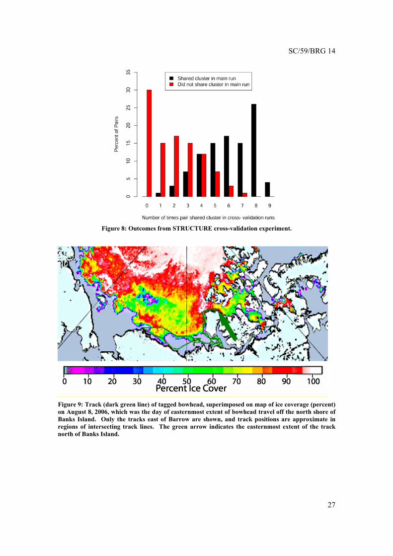
SC/59/BRG 14

27

Figure 8: Outcomes from STRUCTURE cross-validation experiment.

Figure 9: Track (dark green line) of tagged bowhead, superimposed on map of ice coverage (percent) on August 8, 2006, which was the day of easternmost extent of bowhead travel off the north shore of Banks Island. Only the tracks east of Barrow are shown, and track positions are approximate in regions of intersecting track lines. The green arrow indicates the easternmost extent of the track north of Banks Island.

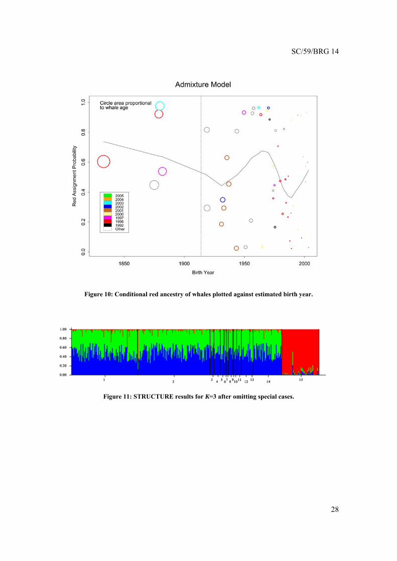
SC/59/BRG 14

28

Figure 10: Conditional red ancestry of whales plotted against estimated birth year.

Figure 11: STRUCTURE results for K=3 after omitting special cases.