pattern recognition and machine learning · pattern recognition and machine learning ... questions...

PATTERN RECOGNITION ANDMACHINE LEARNING

Slide Set 3: Detection Theory

January 2018

Heikki [email protected]

Department of Signal ProcessingTampere University of Technology

mailto:[email protected]

Detection theory

� In this section, we will briefly consider detection theory.� Detection theory has many common topics with machine learning.� The methods are based on estimation theory and attempt to answer

questions such as� Is a signal of specific model present in our time series? E.g., detection of noisy

sinusoid; beep or no beep?� Is the transmitted pulse present at radar signal at time t?� Does the mean level of a signal change at time t?� After calculating the mean change in pixel values of subsequent frames in

video, is there something moving in the scene?� Is there a person in this video frame?

Detection theory

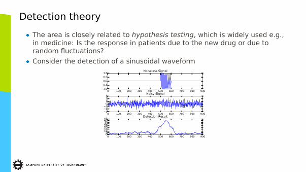
� The area is closely related to hypothesis testing, which is widely used e.g.,in medicine: Is the response in patients due to the new drug or due torandom fluctuations?

� Consider the detection of a sinusoidal waveform

0 100 200 300 400 500 600 700 800 9001.0

0.5

0.0

0.5

1.0Noiseless Signal

0 100 200 300 400 500 600 700 800 9003210123

Noisy Signal

0 100 200 300 400 500 600 700 800 90005

1015202530354045

Detection Result

Detection theory

� In our case, the hypotheses could be

H1 : x[n] = A cos(2πf0n+ ϕ) +w[n]

H0 : x[n] = w[n]

� This example corresponds to detection of noisy sinusoid.� The hypothesis H1 corresponds to the case that the sinusoid is present and

is called alternative hypothesis.� The hypothesis H0 corresponds to the case that the measurements

consists of noise only and is called null hypothesis.

Introductory Example

� Neyman-Pearson approach is the classical way of solving detectionproblems in an optimal manner.

� It relies on so called Neyman-Pearson theorem.� Before stating the theorem, consider a simplistic detection problem, where

we observe one sample x[0] from one of two densities: N (0,1) or N (1,1).� The task is to choose the correct density in an optimal manner.� Our hypotheses are now

H1 : μ = 1,H0 : μ = 0,

and the corresponding likelihoods are plotted below.


4 3 2 1 0 1 2 3 4x[0]

0.00

0.05

0.10

0.15

0.20

0.25

0.30

0.35

0.40

Like

lihood

Likelihood of observing different values of x[0] given H0 or H1

p(x[0] | H0 )

p(x[0] | H1 )

� An obvious approach for deciding the density would choose the one, whichis higher for a particular x[0].

� More specifically, study the likelihoods and choose the more likely one.


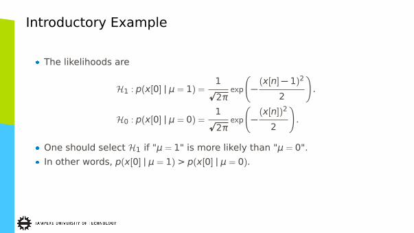
� The likelihoods are

H1 : p(x[0] | μ = 1) =1p

2πexp

�

−(x[n]− 1)2

2

�

.

H0 : p(x[0] | μ = 0) =1p

2πexp

�

−(x[n])2

2

�

.

� One should select H1 if "μ = 1" is more likely than "μ = 0".� In other words, p(x[0] | μ = 1) > p(x[0] | μ = 0).


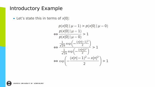
� Let’s state this in terms of x[0]:

p(x[0] | μ = 1) > p(x[0] | μ = 0)

⇔p(x[0] | μ = 1)

p(x[0] | μ = 0)> 1

⇔1p2π

exp�

− (x[n]−1)2

2

�

1p2π

exp�

− (x[n])2

2

� > 1

⇔ exp

�

−(x[n]− 1)2 − x[n]2

2

�

> 1


⇔ (x[n]2 − (x[n]− 1)2) > 0⇔2x[n]− 1 > 0

⇔ x[n] >1

2.

� In other words, choose H1 if x[0] > 0.5 and H0 if x[0] < 0.5.� Studying the ratio of likelihoods on the second row of the derivation is the

key.� This ratio is called likelihood ratio, and comparison to a threshold γ (hereγ = 1) is called likelihood ratio test (LRT).

� Of course the threshold γ may be chosen other than γ = 1.

Error Types

� It might be that the detection problem is not symmetric and some errorsare more costly than others.

� For example, when detecting a disease, a missed detection is more costlythan a false alarm.

� The tradeoff between misses and false alarms can be adjusted using thethreshold of the LRT.

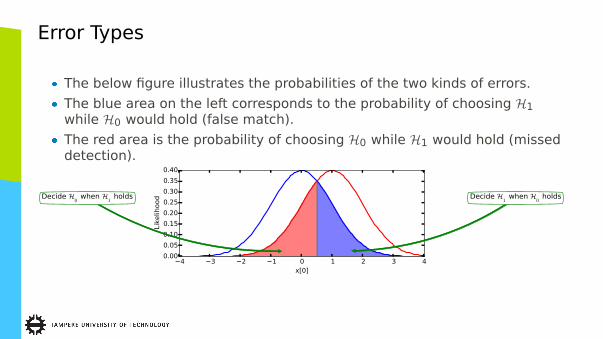
Error Types

� The below figure illustrates the probabilities of the two kinds of errors.� The blue area on the left corresponds to the probability of choosing H1

while H0 would hold (false match).� The red area is the probability of choosing H0 while H1 would hold (missed

detection).

4 3 2 1 0 1 2 3 4x[0]

0.00

0.05

0.10

0.15

0.20

0.25

0.30

0.35

0.40

Like

lihoodDecide H

0 when H

1 holds Decide H

1 when H

0 holds

Error Types

� It can be seen that we can decrease either probability arbitrarily small byadjusting the detection threshold.

4 3 2 1 0 1 2 3 4x[0]

0.00

0.05

0.10

0.15

0.20

0.25

0.30

0.35

0.40

Like

lihoodDecide H

0 when H

1 holds Decide H

1 when H

0 holds

Detection threshold at 0. Small amount of misseddetections (red) but many false matches (blue).

4 3 2 1 0 1 2 3 4x[0]

0.00

0.05

0.10

0.15

0.20

0.25

0.30

0.35

0.40

Like

lihoodDecide H

0 when H

1 holds Decide H

1 when H

0 holds

Detection threshold at 1.5. Small amount of falsematches (blue) but many missed detections (red).

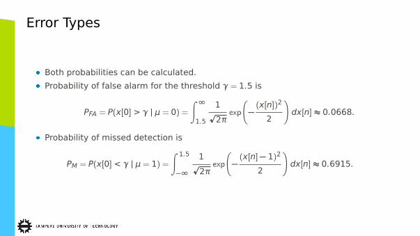
Error Types

� Both probabilities can be calculated.

� Probability of false alarm for the threshold γ = 1.5 is

PFA = P(x[0] > γ | μ = 0) =∫ ∞

1.5

1p

2πexp

�

−(x[n])2

2

�

dx[n] ≈ 0.0668.

� Probability of missed detection is

PM = P(x[0] < γ | μ = 1) =∫ 1.5

−∞

1p

2πexp

�

−(x[n]− 1)2

2

�

dx[n] ≈ 0.6915.

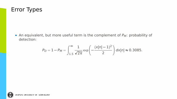
Error Types

� An equivalent, but more useful term is the complement of PM: probability ofdetection:

PD = 1− PM =

∫ ∞

1.5

1p

2πexp

�

−(x[n]− 1)2

2

�

dx[n] ≈ 0.3085.

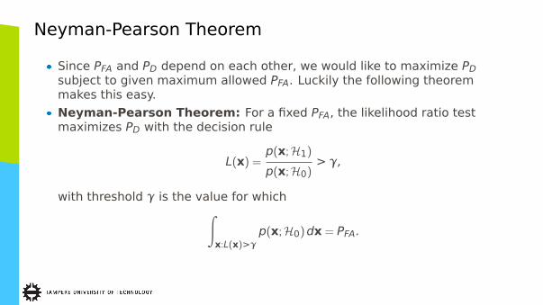
Neyman-Pearson Theorem

� Since PFA and PD depend on each other, we would like to maximize PDsubject to given maximum allowed PFA. Luckily the following theoremmakes this easy.

� Neyman-Pearson Theorem: For a fixed PFA, the likelihood ratio testmaximizes PD with the decision rule

L(x) =p(x;H1)

p(x;H0)> γ,

with threshold γ is the value for which∫

x:L(x)>γp(x;H0)dx = PFA.


� As an example, suppose we want to find the best detector for ourintroductory example, and we can tolerate 10% false alarms (PFA = 0.1).

� According to the theorem, the detection rule is:

Select H1 ifp(x | μ = 1)

p(x | μ = 0)> γ

The only thing to find out now is the threshold γ such that∫ ∞

γp(x | μ = 0)dx = 0.1.


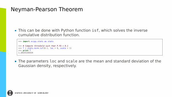
� This can be done with Python function isf, which solves the inversecumulative distribution function.>>> import scipy.stats as stats

>>> # Compute threshold such that P_FA = 0.1>>> T = stats.norm.isf(0.1, loc = 0, scale = 1)>>> print T1.28155156554

� The parameters loc and scale are the mean and standard deviation of theGaussian density, respectively.

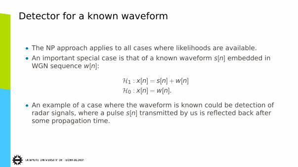
Detector for a known waveform

� The NP approach applies to all cases where likelihoods are available.� An important special case is that of a known waveform s[n] embedded in

WGN sequence w[n]:

H1 : x[n] = s[n] +w[n]

H0 : x[n] = w[n].

� An example of a case where the waveform is known could be detection ofradar signals, where a pulse s[n] transmitted by us is reflected back aftersome propagation time.


� For this case the likelihoods are

p(x | H1) =N−1∏

n=0

1p

2πσ2exp

�

−(x[n]− s[n])2

2σ2

�

,

p(x | H0) =N−1∏

n=0

1p

2πσ2exp

�

−(x[n])2

2σ2

�

.

� The likelihood ratio test is easily obtained as

p(x | H1)

p(x | H0)= exp

�

−1

2σ2

�N−1∑

n=0

(x[n]− s[n])2 −N−1∑

n=0

(x[n])2

��

> γ.


� This simplifies by taking the logarithm from both sides:

−1

2σ2

�N−1∑

n=0

(x[n]− s[n])2 −N−1∑

n=0

(x[n])2

�

> lnγ.

� This further simplifies into

1

σ2

N−1∑

n=0

x[n]s[n]−1

2σ2

N−1∑

n=0

(s[n])2 > lnγ.


� Since s[n] is a known waveform (= constant), we can simplify the procedureby moving it to the right hand side and combining it with the threshold:

N−1∑

n=0

x[n]s[n] > σ2 lnγ+1

2

N−1∑

n=0

(s[n])2.

We can equivalently call the right hand side as our threshold (say γ′) to getthe final decision rule

N−1∑

n=0

x[n]s[n] > γ′.

Examples

� This leads into some rather obvious results.� The detector for a known DC level in WGN is

N−1∑

n=0

x[n]A > γ⇒ AN−1∑

n=0

x[n] > γ

Equally well we can set a new threshold and call it γ′ = γ/(AN). This waythe detection rule becomes: x > γ′. Note that a negative A would invertthe inequality.

Examples

� The detector for a sinusoid in WGN is

N−1∑

n=0

x[n]A cos(2πf0n+ ϕ) > γ⇒ AN−1∑

n=0

x[n] cos(2πf0n+ ϕ) > γ.

� Again we can divide by A to get

N−1∑

n=0

x[n] cos(2πf0n+ ϕ) > γ′.

� In other words, we check the correlation with the sinusoid. Note that theamplitude A does not affect our statistic, only the threshold which isanyway selected according to the fixed PFA rate.

Examples

� As an example, the below picture shows the detection process with σ = 0.5.

0 100 200 300 400 500 600 700 800 9001.0

0.5

0.0

0.5

1.0Noiseless Signal

0 100 200 300 400 500 600 700 800 9003210123

Noisy Signal

0 100 200 300 400 500 600 700 800 900

40200

2040

Detection Result

Detection of random signals

� The problem with the previous approach was that the model was toorestrictive; the results depend on how well the phases match.

� The model can be relaxed by considering random signals, whose exactform is unknown, but the correlation structure is known. Since thecorrelation captures the frequency (but not the phase), this is exactly whatwe want.

� In general, the detection of a random signal can be formulated as follows.� Suppose s ∼ N (0,Cs) and w ∼ N (0, σ2I). Then the detection problem is a

hypothesis test

H0 : x ∼ N (0, σ2I)

H1 : x ∼ N (0,Cs + σ2I)

Detection of random signals

� It can be shown, that the decision rule becomes

Decide H1, if xT s > γ,

wheres = Cs(Cs + σ2I)−1x.

Example of Random Signal Detection

� Without going into the details, let’s jump directly to the derived decisionrule for the sinusoid:

�

�

�

�

�

N−1∑

n=0

x[n] exp(−2πif0n)

�

�

�

�

�

> γ.

� As an example, the below picture shows the detection process with σ = 0.5.� Note the simplicity of Python implementation:

import numpy as np

h = np.exp(-2 * np.pi * 1j * f0 * n)y = np.abs(np.convolve(h, xn, ’same’))

Example of Random Signal Detection

0 100 200 300 400 500 600 700 800 9001.0

0.5

0.0

0.5

1.0Noiseless Signal

0 100 200 300 400 500 600 700 800 9003210123

Noisy Signal

0 100 200 300 400 500 600 700 800 90005

1015202530354045

Detection Result

Receiver Operating Characteristics

� A usual way of illustrating the detector performance is the ReceiverOperating Characteristics curve (ROC curve).

� This describes the relationship between PFA and PD for all possible values ofthe threshold γ.

� The functional relationship between PFA and PD depends on the problemand the selected detector.


� For example, in the DC level example,

PD(γ) =

∫ ∞

γ

1p

2πexp

�

−(x− 1)2

2

�

dx

PFA(γ) =

∫ ∞

γ

1p

2πexp

�

−x2

2

�

dx

� It is easy to see the relationship:

PD(γ) =

∫ ∞

γ−1

1p

2πexp

�

−x2

2

�

dx = PFA(γ − 1).


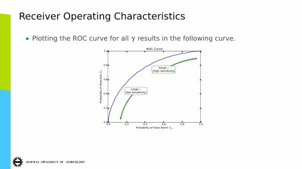
� Plotting the ROC curve for all γ results in the following curve.

0.0 0.2 0.4 0.6 0.8 1.0Probability of False Alarm PFA

0.0

0.2

0.4

0.6

0.8

1.0

Pro

babili

ty o

f D

ete

ctio

n P

D

Small γ(high sensitivity)

Large γ(low sensitivity)

ROC Curve


� The higher the ROC curve, the better the performance.� A random guess has diagonal ROC curve.� This gives rise to a widely used measure for detector performance: theArea Under (ROC) Curve, or AUC criterion.

� The benefit of AUC is that it is threshold independent, and tests theaccuracy for all thresholds.

� In the DC level case, the performance increases if the noise variance σ2

decreases (since the problem becomes easier).� Below are the ROC plots for various values of σ2.



0.0

0.2

0.4

0.6

0.8

1.0

Pro

babili

ty o

f D

ete

ctio

n P

D

σ = 0.2 (AUC = 1.00)σ = 0.4 (AUC = 0.96)σ = 0.6 (AUC = 0.88)σ = 0.8 (AUC = 0.81)σ = 1.0 (AUC = 0.76)

Random Guess (AUC = 0.5)

Empirical AUC

� Initially, AUC and ROC stem from radar and radio detection problems.� More recently, AUC has become one of the standard measures of

classification performance, as well.� Usually a closed form expression for PD and PFA can not be derived.� Thus, ROC and AUC are most often computed empirically; i.e., by

evaluating the prediction results on a holdout test set.

Classification Example—ROC and AUC

� For example, consider the 2-dimensional dataset on theright.

� The data is split to training and test sets, which are similarbut not exactly the same.

� Let’s train 4 classifiers on the upper data and compute theROC for each on the bottom data.

2 1 0 1 2 3 4 5 610

8

6

4

2

0

2Training Data

2 1 0 1 2 3 4 5 610

8

6

4

2

0

2Test Data


� A linear classifier trained with the training dataproduces the shown class boundary.

� The class boundary has the orientation andlocation that minimizes the overallclassification error for the training data.

� The boundary is defined by:

y = c1x+ c0

with parameters c1 and c0 learned from data.

2 1 0 1 2 3 4 5 610

8

6

4

2

0

2

Class Boundary

13.5 % of circlesdetected as cross

5.0 % of crossesdetected as circle

Classifier with minimum error boundary


� We can adjust the sensitivity of classification by movingthe decision boundary up or down.

� In other words, slide the parameter c0 in

y = c1x+ c0

� This can be seen as a tuning parameter for plotting theROC curve.

2 1 0 1 2 3 4 5 610

8

6

4

2

0

2

Class Boundary



Classifier with boundary lifted up

2 1 0 1 2 3 4 5 610

8

6

4

2

0

2

Class Boundary



Classifier with boundary lifted down

Classification Example—ROC and AUC� When the boundary slides from bottom to top, we plot the empirical ROCcurve.

� Plotting starts from upper right corner.� Every time the boundary passes a blue cross, the curve moves left.� Every time the boundary passes a red circle, the curve moves down.


0.0

0.2

0.4

0.6

0.8

1.0

Pro

babili

ty o

f D

ete

ctio

n P

D

Figure on the Right

AUC = 0.98

2 1 0 1 2 3 4 5 610

8

6

4

2

0

2

Class Boundary



Classifier with minimum error boundary


� Real usage is for comparing classifiers.� Below is a plot of ROC curves for 4 widely used classifiers.� Each classifier produces a class membership score over which the tuning

parameter slides.


0.0

0.2

0.4

0.6

0.8

1.0

Pro

babili

ty o

f D

ete

ctio

n P

D

Logistic Regression (AUC = 0.98)Support Vector Machine (AUC = 0.96)Random Forest (AUC = 0.97)Nearest Neighbor (AUC = 0.96)

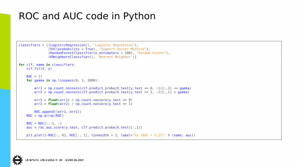
ROC and AUC code in Python

classifiers = [(LogisticRegression(), "Logistic Regression"),(SVC(probability = True), "Support Vector Machine"),(RandomForestClassifier(n_estimators = 100), "Random Forest"),(KNeighborsClassifier(), "Nearest Neighbor")]

for clf, name in classifiers:clf.fit(X, y)

ROC = []for gamma in np.linspace(0, 1, 1000):

err1 = np.count_nonzero(clf.predict_proba(X_test[y_test == 0, :])[:,1] <= gamma)err2 = np.count_nonzero(clf.predict_proba(X_test[y_test == 1, :])[:,1] > gamma)

err1 = float(err1) / np.count_nonzero(y_test == 0)err2 = float(err2) / np.count_nonzero(y_test == 1)

ROC.append([err1, err2])ROC = np.array(ROC)

ROC = ROC[::-1, :]auc = roc_auc_score(y_test, clf.predict_proba(X_test)[:,1])

plt.plot(1-ROC[:, 0], ROC[:, 1], linewidth = 2, label="%s (AUC = %.2f)" % (name, auc))

pattern recognition and machine learning · pattern recognition and machine learning ... questions...

Documents