Pattern inference theory: A probabilistic approach to vision∗

Daniel Kersten and Paul Schrater†

November 21, 1999

∗To be published: Kersten, D., & Schrater, P. W. Pattern inference theory: A probabilistic approach to vision. InMausfeld, R., Heyer, D. (Eds.), Perception and the Physical World (Chichester: John Wiley Sons, Ltd.)

†Department of Psychology, University of Minnesota, Minneapolis, MN. Email: kersten@tc.umn.edu.Supported by NSF SBR-9631682 and NIH RO1 EY11507-001.

1

Abstract

The function of vision is to get correct and useful answers about the state of the world. However,given that the state of the world is not uniquely specified by the visual input, the visual system mustmake good guesses or inferences. Thus, theories of visual system functions will be theories of inference,and we need a language in which theories of inference can be described. Analogous to calculus havinga minimum expressiveness required to formulate theories in physics, we argue that the language ofBayesian inference is fundamental to quantitatively describe how reliable answers about the world can beobtained from image patterns. Bayes provides a minimal formalism that can deal with the sophisticationand versatility of perception missing from some other approaches. Key missing components include theability to model uncertainty, probabilistic modeling of pattern synthesis as a necessary prerequisiteto understanding pattern inference, the means to handle the complexity of natural images, and thediversity of visual tasks.

Most of the formal elements that we describe are not new and have their roots in signal detection theoryand ideal observer analysis. We start from there to review and codify principles drawn from recentapplications of Bayesian decision theory, Bayes nets and pattern theory to vision. To emphasize theimportance of dealing with the complexity of natural image and scene patterns, we call the conjunctionof principles drawn from these contributions pattern inference theory. Because of its generality, we donot see pattern inference theory as an experimentally testable theory of vision; however, it does providea set of concepts and principles to formulate testable models. The test for a good theoretical frameworkis utility and completeness for deriving predictive theories. To illustrate the utility of the approach,we propose Bayesian principles of least commitment and modularity, each of which leads to testablehypotheses. Several recent examples of pattern inference theories are reviewed.

1 Perception is pattern decoding

Few would dispute the view that visual perception is the brain’s process for arriving at useful informationabout the world from images. Divergent opinions, however, have been expressed over how to describethe computations (or lack thereof) underlying visual behavior. Visual perception has been described asunconscious inference [46, 41], reconstruction [20], resonance [37], problem solving [88], computation [72],and more recently as Bayesian inference [60]. In part, the debate gets muddled due to lack of awell-specified explanatory goal and level of abstraction. To clarify, we see the grand challenge to bethe development of testable, quantitative theories of visual performance that take into account thecomplexities of natural images and the richness of visual behavior. But here the level of explanation iscrucial: if our theories are too abstract, we lose the specificity of quantitative predictions; if the theoriesare too fine-grained, the model mechanisms for natural pattern processing will be too complex to test.

Our proposed strategy follows that of statistical mechanics. Few physicists doubt that the large-scaleproperties of physical systems rest on the lawful function of individual molecules, just as few brainscientists doubt that an organism’s behavior depends on the lawful function of neurons. Physicistswould agree that the modeling level has to be appropriate to the measurements and phenomena oflarge-scale systems; thus statistical mechanics links molecular kinetics to thermodynamics. Althoughthe bridge between neurons and system behavior has yet to be built, the language of Bayesian statistics

2

provides the level of description analogous to thermodynamics 1. For vision, theories at this level aretestable at the level of visual information and perceptual constraints 2, and are less committal aboutrepresentations, algorithms, or mechanisms.

The purpose of this chapter is to describe the fundamental principles of value in addressing the grandchallenge. These principles constitute what we will refer to as pattern inference theory. The basicelements of pattern inference theory are not new and have their mathematical roots in communicationand information theory [95], Bayesian decision theory [11], pattern theory [45], and Bayes nets [79].The refinement of the principles are derived from a history of applications to human vision in thedomains of signal detection theory [40], ideal observer analysis [35, 92], Bayesian inference and decisiontheory [53, 117], and pattern theory [75, 118]. “Pattern theory” was developed by Ulf Grenander todescribe the mathematical study of complex natural patterns [44, 45, 75, 118]. Central features ofpattern theory are the importance of modeling pattern generation, and that natural pattern variationis characterized by four fundamental classes of deformations 3. Further, the generative model is seenas an essential part of inference (e.g. via flexible templates to fit incoming data in a feedback stage) todeal with certain types of deformation, such as occlusion [74]. Our particular emphasis is based on thesynthesis and application of pattern theory and Bayesian decision theory to human vision [118]. As anelaboration of signal detection theory, we choose the words pattern and inference to stress the importanceof modeling complex natural signals, and of considering tasks in addition to detection, respectively. Weargue that pattern inference theory provides the best language for formulating quantitative theories ofvisual perception and action at the level of the naturally behaving (human) visual system.

Our goal is to derive probabilistic models of the observer’s world and sensory input, restricted by task.Such models have two components: the objects of the theory, and the operations of the theory. Theobjects of the theory are the set of possible image measurements I, the set of possible scene descriptionsS, and the joint probability distribution of S and I: p(S, I). The operations are given by the probabilitycalculus, with decisions modeled as minimizing expected cost (or risk) given the probabilities. Therichness of the theory lies in exploiting the structure induced in p(S, I) by the regularities of the world(laws of physics) and by the habits of observers. A fundamental assumption of pattern inference theoryis that Bayesian decision theory provides the best language both to describe complex patterns, and tomodel inferences about them. For us, the essence of a Bayesian view is not the emphasis on subjectiveprior probabilities, but rather that all variables are random variables. This assumption has ramificationsfor the central role, in perception, of generative (or synthetic) models of image patterns, as well as priorprobability models of scene information. An emphasis on generative models, we believe, is essentialbecause of the inherent complexity of the causal structure of high-dimensional image patterns. Onemust model how the multitude of variables (both the needed and unneeded variables for a task) interactto produce image data in order to understand how to decode those patterns. But perhaps equallyimportantly, the Bayesian view underscores the importance of confidence-driven visual processes. Thislatter idea leads us to the view that perception consists of sequences of computations on probabilities,rather than a series of estimations or decisions. We illustrate this with recent work on Bayes nets.

1Our level of analysis falls between the computational/function and representation/algorithmic levels in the Marrhierarchy.

2Because it is rare to find a visual cue that is sufficiently reliable to unambiguously determine a perceived sceneproperty, perception should be viewed as satisfying multiple constraints simultaneously. Examples are the constraint thatlight sources tend to be from above, or that a sharp image edge is more likely a reflectance or depth change than a shadow.

3These four classes are intended to apply generally to natural patterns of all sorts, and not just to visual patterns.For spatial vision, these classes would correspond to: blur and noise, geometric deformations, superposition (e.g. of basisimages), and occlusions [74].

3

In the next section, we will show that pattern inference theory is a logical elaboration of ideal observeranalysis in classical signal detection theory. However, it goes beyond standard applications of idealobserver analysis by emphasizing the need to take into account the full range of natural image patterns,and the intimate tie between perception and successful behavior.

2 Pattern inference theory: A generalization of ideal observers

Signal detection theory (SDT) was developed in the 1950’s to model and analyze human sensory decisionsgiven internal and external background noise [81, 40]. The theory combined earlier work in statisticaldecision theory [77, 112, 111, 42] with communication systems theory [95, 86]. Signal detection theorymade two fundamental contributions to our understanding of human perception. First, statisticaldecision theory showed how to analyze the internal processing of sensory decisions. The applicationof statistical decision theory to psychophysics showed that sensory decisions were determined by twoexperimentally separable factors: sensitivity (related to an inferred internal signal-to-noise ratio) and thedecision criterion. Second, communication theory showed that there were inherent physical limits to thereliability of information transmission, and thus detection, independent of the specific implementation ofthe detector, i.e. whether it be physical or biological. These limits can be modeled by a mathematicallydefined ideal observer, which provides a quantitative computational theory for the information in atask. For the ideal observer, the signal-to-noise ratio can be obtained from direct measurements ofthe variations in the transmitted signal. The ideal observer presaged Marr’s ideas of a computationaltheory for an information processing task, as distinct from the algorithm and implementation to carryit out [72]. The top panel of figure (1) illustrates the basic causal structure for the “signal plus noise”problem in classical signal detection theory.

Experimental studies of human perceptual behavior are often left with a crucial, but unanswered ques-tion: To what extent is the measured performance limited by the information in the task rather than bythe perceptual system itself? Answers to this question are critical for understanding the relationship be-tween perceptual behavior and its underlying biological mechanisms. Signal detection theory providedan answer through ideal observer analysis. One of the first applications of the ideal observer in visionwas the determination of the quantum efficiency of human light discrimination [7]. By considering boththe external and internal sources of variability, Barlow showed that an ideal photon detector could getby with about one tenth the number of photons as a human for the same combination of hit and correctrejection rates. This success of classical signal detection theory demonstrated the need for probabilityin theories of visual performance, because light transmission is fundamentally stochastic (emission andabsorption are Poisson processes) and any real light measurement device introduces further noise.

The example of ideal observer analysis of light detection further illustrates a fundamental strategy forstudying perception, consisting of three modeling domains. First, how does the signal (i.e. light switchset to “bright” or “dim”) get encoded into intensity changes in the image? The answer must deal withlight variations due to quantal fluctuations. Second, how should the received image data be decoded todo the best job at inferring which signal was transmitted? Answers to this question rely on theories ofideal observers, or more generally of optimal inference. Third, how does one compare human and idealperformance? This requires common performance measures on the same task.

4

H =µ

S1

µS2

n ~ N [0,σ ]

x=µsi+n

H=Se Sg

x=φ(Se,Sg)

Figure 1: The top panel shows an example of generative graph structure for an ideal observer problem inclassical signal detection theory (SDT). The data are determined by the signal hypotheses plus (usuallyadditive gaussian) noise. Knowledge is represented by the joint probability p(x, u, n). The lower panelshows a simplified example of the generative structure for perceptual inference from a pattern inferencetheory perspective. The image measurements (x) are determined by a typically non-linear function (φ) ofprimary signal variables (Se) and confounding secondary variables (Sg). Knowledge is represented by thejoint probability p(x, Se, Sg). Both scene and image variables can be high dimensional vectors. In general,the causal structure of natural image patterns is more complex and consequently requires elaboration ofits graphical representation (see Section 3.4). For SDT and pattern inference theory, the task is to make adecision about the signal hypotheses or primary signal variables, while discounting the noise or secondaryvariables. Thus optimal perceptual decisions are determined by p(x, Se), which is derived by summing overthe secondary variables (i.e. marginalizing with respect to the secondary variables):

∫Sg

p(x, Se, Sg)dSg.

2.0.1 Limitations of Signal Detection Theory for the Grand Challenge

Despite its successes, signal detection theory as typically applied in vision falls short when faced with ourgrand challenge. Define perceptual signals to be some underlying causes of image data that are requiredfor a visual behavior. These signals include the shapes, positions, and material of objects. The firstproblem is that natural perceptual signals are complex, high-dimensional functions of image intensities.In typical applications of SDT and classical ideal observer analysis to visual psychophysics, the inputdata, the noise, and the signal, are treated as the same “stuff”. For example, in contrast detection, theinput data is signal plus noise [51]. The signal is based on a physical quantity (luminance) as a functionof time and/or space), the noise is either physical contrast fluctuations, or internal variability treatedas equivalent to the physical noise [80]. Perceptual decisions are typically limited to information whichis explicit in the decoded signal. So to answer the question, Does the signal image have more lightintensity than another?, the decoder simply measures whether the image intensity is bigger.

We need a theoretical framework for which the signals can be any properties of the world useful for thevisual behavior; for example, estimates of object shape and surface motion are crucial for actions such asrecognition and navigation, but they are not simple functions of light intensity. Natural images are high-dimensional functions of useful signals, and arriving at decoding functions relating image measurementsto these signals is a major theoretical challenge. Both of these problems are expressible in terms ofpattern inference theory.

In signal detection theory, the non-signal causes of the input pattern are called noise. A second problem,related to the first, is that “noise” in the perception of natural images is not simple. Useful informationis confounded by more than added external or internal image intensity noise. Uncertainty is due to

5

both variations in unneeded scene variables as well as by the fact that multiple scene descriptions canproduce the same image data. In contrast to the above example of contrast detection, consider theproblem of 3D shape discrimination in everyday vision. The signal is shape, but the counterpart to thenoise is very different stuff, and includes variation in viewpoint, illumination, other occluding objects,and material [68]. Further, although the discrimination decision may be able to rely on a primary imagemeasurement that is explicit in the image (e.g. a contour description), this is rare. Because of projectionand the confounding variables, the true 3D shape is not explicit in any simple image measurement.

Pattern inference theory deals directly with the problem of multiple and diverse causes of image varia-tion by modeling the generative process of image formation. Below, we distinguish between the neededprimary and unneeded secondary variables.4 The primary variables are those which the system’s func-tion is designed to estimate. By contrast, the secondary variables are not estimated but neither arethey ignored, and there are principled methods for getting rid of unwanted variables. It should beemphasized that the distinction between primary and secondary depends on the specific task the sys-tem is designed to solve. Variables which are secondary for one task may be primary for another. Forexample, estimating the illumination is unimportant for many visual tasks and so illumination variablesare treated as secondary. The theory of generic views treats viewpoint as a secondary variable, enablingresolution of ambiguities in shape perception [76, 32]. Light direction as a secondary variable can beused to obtain a unique estimate of depth from cast shadows [56]. There is a close connection betweenthe task (discussed in Section 4 below) and the statistical structure of the estimation problem [93].

A third limitation is that natural images are not linear combinations of their signals, and that theprobabilities describing the signal and image variables are not gaussian. Much of the success of signaldetection theory has rested on an assumption of linearity: the input is the sum of the signal and thenoise. Except in rare instances (e.g. contrast detection limited by photon fluctuations at high lightlevels), natural perceptual tasks involve inputs which are non-linear functions of the signals and thenoise (or secondary variables). For example, light intensity is a non-linear function of object shape,reflectance, and illumination.

There is a close relationship between linearity and the assumption that the random variables of in-terest are Gaussian 5. Although classical signal detection explored the implications of non-Gaussianprocesses [27], most applications of signal detection theory to vision have typically approximated noisevariations as Gaussian processes. A Gaussian approximation works very well in certain domains (as anapproximation to Poisson light emission), but is extremely limited as a model of scene variability. Boththe linear and Gaussian assumptions have had a striking success in the general problem of modelinghuman perceptual and cognitive decisions, where the variability is inside the observer [40, 101]. Butthe Gaussian assumption generally fails when modeling external variability. For example, whenevera probability density involves more than second-order correlations, a multi-variate Gaussian model isno longer adequate. Image samples from Gaussian models of natural images fail to capture the richstructure of natural textures [59]. Simple image measurements, such as those made by simple cells ofthe visual cortex are highly non-Gaussian [29]. A goal of pattern inference theory is to let the visionproblem determine the distributions.

Fourthly, perception involves more tasks than classification. Not surprisingly, for signal detection theory,the primary focus is on signal detection–was the signal sent or not? Perception involves a larger class oftasks: classification at several levels of abstraction, estimation, learning, and control. Past applications

4Primary and secondary variables have also been referred to as explicit and generic (or nuisance) variables, respectively.5Because the log of a multi-variate Gaussian is quadratic, extrema can be found using linear estimators.

6

of signal detection theory have successively handled certain kinds of abstraction (e.g. “is any one of 100signals there or not?” or “which of 100 known signals was sent?”) as well as estimation [107]; but we alsorequire a framework that can handle diverse tasks from continuous estimations (e.g. of distance, shape,and their associations) to more complex categorical decisions: e.g. is the input pattern due to a cat, adog, or “my cat”? Tools for the former build on classical estimation theory, but include recent work onhidden markov models. The latter requires additional tools, such as flexible template theories to modelshape abstraction. A mathematical framework for perception requires tools for the generalization ofideal observers for the functional complex tasks of natural perception. Defining primary and secondaryvariables is part of task specification, and pattern inference theory handles this by incorporating decisiontheory to define a risk function (Section 4).

Finally, we note that most of the interesting perceptual knowledge on priors and utility is implicit.Signal detection theory grew out of earlier work on decision theory. Two important components ofdecision theory are the specification of prior probabilities of scene properties or signals and the costsand benefits of actions, through a risk or cost function. In most applications of SDT, it has beenthe experimenter that manipulates the priors and the cost functions. The human observer is oftenaware of the changes, and can adopt a conscious strategy to take these into account. We argue thatthe most important perceptual priors are largely determined by the structure of the environment andcan, in principle, be modeled independently of perceptual inference (i.e. in the synthesis phase ofstudy)6. Modeling priors (e.g. through density estimation) is a hard theoretical problem in and ofitself, especially because of the large number of potential interactions. In classical SDT, probabilitiesare typically specified over small dimensional spaces. The costs and benefits are inherent to the type ofperceptual task, and determine the primary and secondary variables. Thus, to elaborate on Helmholtz’sdefinition of perception: perception is (largely) unconscious inference involving unconscious priors, andunconscious cost functions.

Thanks to the successes of signal detection theory, we know that perception is limited by two factors:1) the available information for reliable learning, inference, and action; 2) brain mechanisms to processthat information. But one of the principal differences between classical SDT and pattern inferencetheory is the greater emphasis on modeling the external limits to inference, including both synthesisand optimal decoding. Both problems are clearly challenging, and computer vision has shown that thesecond problem is surprisingly hard. We agree with Marr when he wrote in 1982: “...the nature of thecomputations that underlie perception depends more upon the computational problems that have to besolved than upon the particular hardware in which their solutions are implemented.” Theories of humanperceptual inference require an understanding of the limits of perceptual inference through optimaldecoding theories [8, 35]. These theories, in turn, require an understanding of the transformationsand variations introduced in pattern formation. We will argue here that the structure of the visualinformation for function is best modeled in terms of its probabilistic structure, and that as a consequenceany successful system must reflect the constraints in that structure, and further that its computationsshould be in terms of probability operations.

So, in the next section, we focus on the first problem: How can we model the information requiredfor a task? This modeling problem can be broken down into: a) synthesis, modeling the structure ofpattern information in natural images; and b) analysis, modeling the task and extracting useful patternstructures.

6We emphasize an empirical Bayesian approach in which, as is discussed in Section 6, one can test an hypothesis relatinga subjective prior to an objective prior.

7

3 Encoding of scenes in images: Modeling image pattern synthesis

Computer vision has emphasized the difficulty of image understanding, which involves decoding imagesto find the scene variables causing the image measurements. Although, a great deal of progress hasbeen made in computer vision, the best systems are typically quite constrained in their domain ofapplicability (e.g. letter recognition, tracking, structure from rigid body motions, etc.). The focus hasunderstandably been on decoding–e.g. solving the inverse optics problem. However, the success of imagedecoding depends crucially on understanding the encoding. Although the computational challenge ofimage understanding is widely appreciated, the difficulty and issues of image pattern synthesis are lessso.

How do we model the information images contain about scene properties? Following Shannon (1949),the answer is through probability distributions. Treating perception as a communication problem, weidentify certain scene variables S as the messages, and the image formation and measurement mappingas the channel p(I|S), by which we receive the encoded messages I. Given this identification, we canuse information theoretic ideas to quantify the information that I gives about S as the transinformation

I(S; I) = H(I) −H(I|S) = Ep(I)[− log p(I)] − Ep(S,I)[− log p(I|S)].

These entropies are determined by p(I) =∫S p(S)p(I|S)dS, the likelihood p(I|S), and the prior p(S).7

Thus, the physics of materials, optics, light, and image measurement, which determine the likelihood,just scratch the surface of what is required to model image encoding. In addition, we need to understandthe types of patterns and transformations that result from the fact that images are caused by a structuredworld of events and potentialities for an agent, which is captured in p(S). While probability andinformation theory provide the tools for understanding image encoding, constructing theories withthese tools requires work. Let’s look at the framework, tools, and principles for theory construction.

3.1 Essence of Bayes: Everything is a random variable

A key starting assumption is that all variables are random variables, and that the knowledge required forvisual function is specified by the joint probability p(Se, Sg, I). The basic ingredients are variable classes:image measurement data (I), variables specifying relevant scene attributes (Se), and the confoundingvariables (Sg). All these variables are random variables, and thus subject to the laws of the probabilitycalculus, including Bayes theorem. So for pattern inference theory, a Bayesian view is more thanacknowledging the role of priors, but also emphasizes the redundancy structure of images, and theimportance of the generative process of visual pattern formation, expressible as a graphical model. Thusthe essence of a Bayesian theory of perception is more than applying Bayes’ rule to infer scene propertiesfrom images, or that likelihoods are tweaked by prior and labile subjective “biases”. This interpretation

7For simplicity, we’ve restricted our expressions to probability densities on continuous random, rather than discrete,random variables. There are well-known subtleties in translating results between discrete probabilities and continuousdensities. Examples: 1) A change of representation (e.g. changing distance to vergence angle) will in general change theform of the density–e.g. change a uniform density into a non-uniform one. 2) Entropy for continuous variables is inherentlyrelative, and thus transinformation is more useful [22]. 3) If the range of a random variable is unknown, then the principleof insufficient reason leads to “improper” priors [11].

8

(Myth 1: Bayesian models of perception are distinct only by virtue of emphasis on modeling priors8)would miss the point of our view of pattern inference theory approach to perception. By starting witha model space completely determined by the joint probability, p(Se, Sg, I), we have the foundation tounderstand:

1) input image redundancy, through:

p(I) =∫

p(Se, Sg, I) dSe dSg

2) scene structure, through:

p(Se, Sg) =∫

p(Se, Sg, I)dI

and

3) inference, through:

p(Se, I) =∫

p(Se, Sg, I)dSg

.

Of course, modeling p(Se, Sg, I) in general may pose an insurmountable challenge. But there is reasonfor optimism, and recent work in density estimation and image statistics suggest that tractable high-dimensional models may be possible [121, 122, 123, 98, 99].

The key point is that necessary knowledge to characterize the perceptual problem is specified by a jointprobability over the given data (usually image measurements, but could include contextual conclusionsdrawn earlier or elsewhere), what the visual system needs (primary), and the variables that confound(secondary variables).

3.2 Basic operations on probabilities: Conditioning and Marginalizing

We really have only two basic computations on probabilities, which follow from the two basic rules ofprobability–the sum and product rules. Each of the rules has specific roles in an inference computation,related to the kind of variable in the inference. When inferring the values of a set of variables Se, theremaining variables come in two types: those which we don’t know and don’t care to know, and thosewhich are known either by sensory measurement or a priori. How is the joint probability affected bythis knowledge? The answer is to sum over the unneeded variables (marginalization), and divide thejoint by the probability of the known ones (conditioning).

1) Marginalization: Presuming the utility of only a subset of the scene variables (which we treat inSection 4), the values of some variables Sg are not known, and we don’t care to know them. Marginal-ization is the proper way to remove the effect of these secondary, unknown, unwanted variables:

8At several points in this chapter, we address what we see as misconceptions of the Bayesian framework for vision. Weidentify these as “myths”.

9

P (Se, I) =∫

Sg

P (Se, Sg, I)dSg

The reason we marginalize is that being unneeded doesn’t mean these variables should be ignored!Most of the time, the unwanted variables (e.g. viewpoint) crucially contribute to the generation of thepossible images, and hence cannot be ignored. The marginalization approach contrasts with traditionalmodular studies of vision, in which most of the unneeded variables for a given module are left out ofthe discussion entirely (e.g. independent estimation of reflectance, shape, and illumination). Often,the modularity is adopted based on general practical and theoretical arguments. Our position is notthat we forgo modularity, but rather that modularity be grounded in the statistical structure of theproblem, rather than by what the theorist finds convenient [93]. It is important to emphasize that thisapproach does not necessitate that marginalizations are executed on-line by the brain. The effects ofmarginalization could be built directly into the inference algorithm avoiding the need for perception tohave an explicit representation of the unneeded variables.

2) Conditioning: Some of our variables are known, through data measurements, or a priori assump-tions. In either case, once we know something about the variables, we base our inferences on thisknowledge by conditioning the joint distribution on the known information:

P (S|I) = P (S, I)/P (I)

The way Bayes’ rule comes into the picture is that it is often easier to separately model image formationand the prior model for the causal factors. Bayes’ rule is a straightforward application of the productrule to P (S, I) = P (I|S)P (S):

P (S|I) = P (I|S)P (S)/P (I)

The likelihood P (I|S) is determined by the generative image formation model which produces imagemeasurements from a scene description. The generative model produces the image patterns, and consistsof the scene prior, and the image formation model. The likelihood is easier to model because we areconditioning on the scene, and the image is a well-defined function of the scene–forward optics plusmeasurement noise. Although the likelihood and prior terms are logically separable, the division haslittle bearing on the algorithmic implementation. When it comes to inference, Bayes is neutral withrespect to whether a priori knowledge is used in a bottom-up or top-down fashion (Myth 2: Priorsare top-down.). The regularizers in computer vision can be expressed as priors, and these are typicallyinstantiated as bottom-up constraints (e.g. weights in feedforward networks [82, 83]).

Why should scene variables be treated probabilistically? In contrast to subjective Bayesian applications(Myth 3: Priors only refer to subjective, and perhaps conscious biases.), prior probabilities on scenevariables are objectively quantifiable. They result from physical processes (e.g. material propertiessuch as albedo and plasticity covary due to common dependence on the substance, such as metal), andfrom the relative frequencies of the scene variables in the observer’s environment. Thus, vision modelershave a big advantage over stock market analysts: they have a better idea of what the functionallyimportant scene causes are, and can hypothesize and test probability density models of scene variables,independent of visual inference. They can also test the extent to which vision respects the constraintsin the prior model (see Section 6). Why is probability essential for modeling pattern synthesis? Because

10

an infinite set of scenes can produce a given image. Thus, in the decoding problem it is essential tohave a model of the generative structure of images, given by p(S|I) and p(S). Below we discuss howseveral kinds of generative processes produce characteristic image patterns.

3.3 Generative models in vision

Functional vision depends on the kind of abstraction required for the task at hand. But psychologicalabstractions such as scene categories, object concepts, and affordances rest on the existence of objectiveworld structure. Without such structure, there would be no support for reliable inferences–in fact,there would be no basis for consistent action in a world in which each image is independent of anyprevious ones. From this perspective, it is not unreasonable for an otherwise functional visual system tohallucinate in response to visual noise, because the best world interpretations will be structured. Thus,understanding the objective generative structure is necessary although not sufficient for an account ofhuman visual perception9. However, a central theme of this chapter is the importance of understandingthe objective generative processes of the images received. It is an intriguing scientific question as tothe degree with which perceptual inference mechanisms mirror or recapitulate the generative imagestructure. Theories of back-projections in visual cortex rest on internal generative processes to dealwith “explaining away” [23, 47] (see Section 4.3), the related idea of model validation through residualcalculation [73, 74], and predictive coding [84]. As we discuss later, the task itself refines our model ofthe relevant statistical structure through Bayesian modularity.

Visual perception deals with two broad classes of generative processes that produce photometric andgeometric image variation. Further, it is useful to distinguish scene variations (knowledge in p(S))from those of image formation (knowledge in p(I|S)). We postpone the discussion of the experimentalimplications of these variations until Section 6.

3.3.1 Object and scene variations

A logical prerequisite for a full understanding of image variation is a study of the nature of illumination,surface reflectivities, object geometry, and scene structure quite independently of the properties of thesense organs. Consider geometrical object variations that occur for a single object. An individualobject, such as a pair of scissors, or a particular human body consists of parts with a range of possiblearticulations. The modeling problem is of significant interest in computer graphic synthesis becauseit provides the means to model the transformations, and ultimately characterize the probabilities ofparticular articulations and actions.

Objects (and scenes) can be categorized at more abstract levels, such as “dogs” or “books” [13, 89].Examples of sources of within-class scatter include geometric variations that occur between differentmembers of the same species, vehicles, or computer keyboards. Certain types of within-class geometricvariation (e.g. “cats”) can be modeled in terms of prototypes together with a description of geometricdeformations [43, 116, 75] which admit a probability measure p(S). For this sort of within-class variation,it may be possible to find p(S) through probability density estimation on scene descriptions. Estimatingprior densities (e.g. via Principal Components Analysis or PCA) for the distribution of facial surfaces(variations across human face shapes) is now possible due to advances in technology for measuring depth

9This is one way of distinguishing the Bayesian perspective from a strict Gibsonian view which could be interpreted asassuming that objective structure is also sufficient to explain functional vision.

11

Figure 2: Illustrations of variations in scene variables. Top left: Group of dogs shows variations ingeometric (size, shape), albedo (shading patterns), and articulation. Top right: Twin dogs show the effectof pose/articulation. Bottom left: A flat-tailed Gecko hides on a tree, showing how variation in skinpigment (albedo) can match the pattern caused by fungus growing on the tree. Bottom Right: A rockystream illustrates the complexities of spatial layout. Rocks come in two size types, large very near thestream, and smaller away from the stream bed. The presence and directionality of the water is encodedin the complex array of specularities, determined by the interaction between light source, water surfacefluctuation, and viewpoint.

12

viewpoint

shadows transparency

occlusion

Figure 3: Variations in illumination and viewing. Top Left: A women’s face shows a shading variationdue to extrinsic shadows. Top Right: Reflection of a house on a window creates a transparent image on acurtain. Bottom Left: Two views of the entrance to Notre Dame Cathedral. Bottom right: A frog hidesunderneath some pond growth, illustrating occlusion/background clutter.

13

maps [4, 109]. Material or albedo variation also occurs across an object set–e.g. the set of books, withdifferent covers. And of course there are mixtures of geometrical and photometrical effects, such aswithin-species variation among dogs. There is a considerable body of work on biological morphometricswhose goal is to understand the transformations connecting objects within groups [16, 17, 50]. Originof concepts at certain levels may lie in the generative structure of objects, and debate has occurredas to whether an entry-level object concept is based on a prototype with (possibly) a metric model ofvariation, or a description of the structural relationships between parts. We touch on this point laterin the context of object recognition models.

“Schemas” are an example of an even higher level of organization involving spatial layout, which rec-ognizes the spatial relationships between objects, and their contextual contingencies. The fact thatperceptual judgments are strongly influenced by scene context, (e.g. forest, office, or grocery storescene), suggests that p(S) is not at all uniform across spatial layout, but rather is highly ‘spiked’ whichallows scene type recognition and its exploitation for scene analysis. See figure 2 for examples of scenevariable variations.

3.3.2 Effects in the image

At the most proximal stage, the images projected into the eyes are transformed by the optics, sampledby the retina, and have noise added to them. These operations produce the well-studied photometricvariations of luminance noise and blurring in the images..

Due to the additivity of light and the approximate linearity of reflection, photometric variations due toillumination change are approximately linear so that under fixed view, an arbitrary lighting conditioncan be approximated by the weighted sum of relatively few basis images [28]. Further, it has been shownthat the images of an object fall on or near a cone in image space [10]. Cast shadows are another formof illumination variation resulting from the occlusion of a light source from a surface. Specularity in animage is an interaction between material, shape, and viewpoint. Surface transparency is another sourceof photometric variation. Its effect in the image can be either additive or multiplicative [54]. One formof additive transparency results from the combination of reflections in a store-front window.

Variations in observer viewpoint (i.e. viewing distance and direction) produce geometric deformationsin the image. The utility of multiple-scale analysis in human and machine vision is in part a consequenceof the distribution of translations in depth of the eye (or camera) viewpoint. Over small changes inviewing variables, the image variations are fairly smooth, although rotations around the viewing spherecan cause large changes in the images due to significant self-occlusions. If we were only concerned withgeometry, viewpoint variations and variation in object position and orientation would produce the sameset of images. However, illumination interacts with viewpoint so that view rotation is only equivalent toobject rotation if the lighting is rigidly attached to the viewer’s frame of reference. Rotations in depthcause particularly challenging image variations for object recognition that we briefly discuss later.

The distribution of multiple objects in a scene affects the images of objects through occlusion andclutter. Because of the nature of imaging, the local correlations in surface features typically carryover to local image features. However, occlusion of one object by another breaks up the image intodisconnected patches. Further, patches widely separated in the image can be statistically related, andthe challenge is to link the appropriate image measurements likely to belong to the same objects. Likeocclusion, background is a significant confounding source of image variation that thwarts segmentation.

14

The intensity edges at the bounding contours of an object can vary substantially as the background ischanged, even if the view and lighting remain the same. See figure 3 for examples of illumination andviewing effects on images.

Occlusion is the result of the distribution of the kinds and spatial arrangements of objects within ascene relative to the viewpoint. But the spatial layouts of schemas also generate statisical dependencein images. Temporal variation in images is induced by object motion and observer actions [14]. Thusthe spatio-temporal image distribution is affected by the distribution of observer actions, and objectdynamics (e.g. freeway driving).

3.4 Graphical models of statistical structure

S

I1 I2

S1 S2

I

S L

I

Figure 4: Components of the generative structure for image patterns involve converging, diverging, andintermediate nodes. For example, these could correspond to: multiple (scene) causes {S1, S2} giving riseto the same image measurement, I; one cause, S influencing more than one image measurement, {I1, I2};a scene (or other) cause S, influencing an image measurement through an intermediate variable L.

In general, natural image pattern formation is specified by a high-dimensional joint probability, requiringan elaboration of the causal structure that is more complex than the simplified model in the bottompanel of figure 1. The idea is to represent the probabilistic structure of the joint distribution P (S, I)by a Bayes net [79, 87], which is simply a graphical model that expresses how variables influence eachother. There are just three basic building blocks: converging, diverging, and intermediate nodes. Forexample, multiple (e.g. scene) variables causing a given image measurement, a single variable producingmultiple image measurements, or a cause indirectly influencing an image measurement through anintermediate variable (see figure 4). These types of influence provide a first step towards modeling thejoint distribution and, as we describe in Section 4 below, the means to efficiently compute probabilitiesof the unknown variables given known values.

Influences between variables are represented by conditioning, and a graphical model expresses the condi-tional independencies between variables. Two random variables may only become independent, however,once the value of some third variable is known. This is called conditional independence.10

Using labels to represent variables and arrows to represent conditioning (with a → b indicating b isconditioned on a11), independence can be represented by the absence of connections between variables.For example, if the joint probability p(a, b, c, d, e, f, g) factors by independence into p(a, b, c, d, e, f, g) =p(a)p(b)p(c|d)p(d)p(e|a, b)p(f |b, c)p(g|d), then the variables can be represented by the graph in figure 5.

10Two random variables are independent if and only if their joint probability is equal to the product of their individualprobabilities. Thus, if p(A, B) = p(A)p(B), then A and B are independent. If p(A, B|C) = p(A|C)p(B|C), then A and Bare conditionally independent. When corn prices drop in the summer, hay fever incidence goes up. However, if the jointon corn price and hay fever is conditioned on “ideal weather for corn and ragweed”, the correlation between corn pricesand hay fever drops. Corn price and hay fever symptoms are conditionally independent.

11In graph theory, a is called the parent of b

15

ba dc

e f g

b Module 1 b Module 2

Stereo Example

ba dc

e f g

c Module 1 c Module 2

a = texture modelb = depthc = fixation distanced = convergencee = monocular cue (texture)f = disparityg = proprioception

ba dc

e f g

a)

b) c)

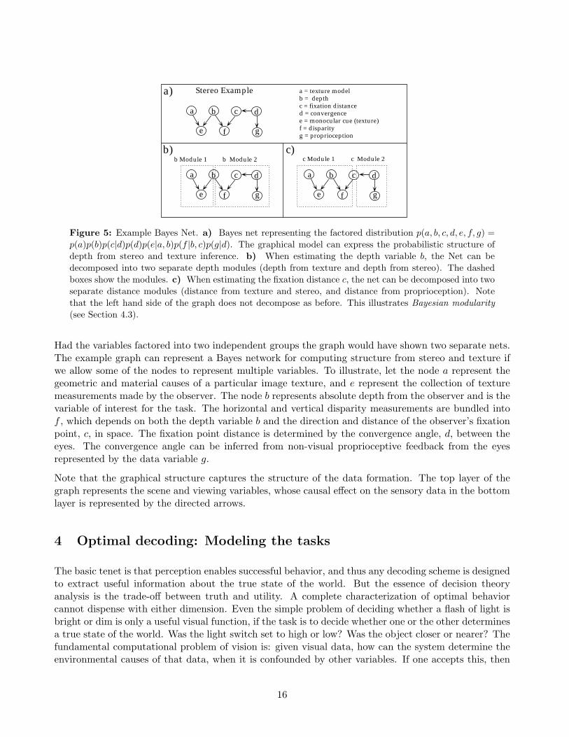
Figure 5: Example Bayes Net. a) Bayes net representing the factored distribution p(a, b, c, d, e, f, g) =p(a)p(b)p(c|d)p(d)p(e|a, b)p(f |b, c)p(g|d). The graphical model can express the probabilistic structure ofdepth from stereo and texture inference. b) When estimating the depth variable b, the Net can bedecomposed into two separate depth modules (depth from texture and depth from stereo). The dashedboxes show the modules. c) When estimating the fixation distance c, the net can be decomposed into twoseparate distance modules (distance from texture and stereo, and distance from proprioception). Notethat the left hand side of the graph does not decompose as before. This illustrates Bayesian modularity(see Section 4.3).

Had the variables factored into two independent groups the graph would have shown two separate nets.The example graph can represent a Bayes network for computing structure from stereo and texture ifwe allow some of the nodes to represent multiple variables. To illustrate, let the node a represent thegeometric and material causes of a particular image texture, and e represent the collection of texturemeasurements made by the observer. The node b represents absolute depth from the observer and is thevariable of interest for the task. The horizontal and vertical disparity measurements are bundled intof , which depends on both the depth variable b and the direction and distance of the observer’s fixationpoint, c, in space. The fixation point distance is determined by the convergence angle, d, between theeyes. The convergence angle can be inferred from non-visual proprioceptive feedback from the eyesrepresented by the data variable g.

Note that the graphical structure captures the structure of the data formation. The top layer of thegraph represents the scene and viewing variables, whose causal effect on the sensory data in the bottomlayer is represented by the directed arrows.

4 Optimal decoding: Modeling the tasks

The basic tenet is that perception enables successful behavior, and thus any decoding scheme is designedto extract useful information about the true state of the world. But the essence of decision theoryanalysis is the trade-off between truth and utility. A complete characterization of optimal behaviorcannot dispense with either dimension. Even the simple problem of deciding whether a flash of light isbright or dim is only a useful visual function, if the task is to decide whether one or the other determinesa true state of the world. Was the light switch set to high or low? Was the object closer or nearer? Thefundamental computational problem of vision is: given visual data, how can the system determine theenvironmental causes of that data, when it is confounded by other variables. If one accepts this, then

16

we can make the case that visual perception is fundamentally image decoding. But whether to drawan inference, or the precision with which it must be drawn is determined by the visual function. Aswith any decoding system, perception operates with target goals that depend on the task. A completetheory of vision needs to account for three classes of behavioral tasks:

1) The visual system draws discrete (categorical) conclusions about objective world. These decisionsinvariably involve taking into account potentially large variations in confounding secondary variables.For example, to reliably detect a face, a system must allow for variations in view, lighting, background,as well as the geometrical variations in individual facial shape, expression, and hair. Finer-grain identi-fications require more estimates of primary variables, and less marginalization with respect to secondaryvariables [55]. Because the causes are objective, decisions have a right or wrong answer. Further, thecost due to incorrect decisions can be large or small. A mistake in animal identification can have seriousconsequences. Failing to anticipate the change in color of a sweater going from indoor to outdoor light-ing may cause only mild social embarrassment, requiring little investment in perceptual (vs. learnedcognitive) resources.

2) The visual system provides continuously valued estimations for actions. For example, visual informa-tion for depth and size determine the kinematics of reach and grasp. Like discrete decisions, estimationscan have degrees of utility.

3) The visual system adapts to environmental contingencies in the images received. This adaptation isat longer time scales than inference required for perceptual problem solving, occurring over both phylo-genetic and ontogenetic scales. One form of adaptation requires implicit probability density estimation.

Can we describe these processes from the point of view of pattern inference theory–i.e. as imagedecoding by means of probability computations? To do so requires a probabilistic model of tasks. Weconsider a task as specifying four things, the required or primary set of scene variables Se, the nuisanceor secondary scene variables Sg, the scene variables which are presumed known Sf , and the decisionto be made. Each of the four components of a task plays a role in determining the structure of theoptimal inference computation. First, we review how to model the decision as a risk functional onthe posterior distribution, then we show that Se and Sf can be used to simplify the joint distributionthrough independence relations, while Sg and the decision rule can make one choice of Se simpler thananother.

Bayesian decision theory provides a precise language to model the costs of errors determined by thechoice of visual task [117, 18]. The cost or risk R(Σ; I) of guessing Σ when the image measurement isI is defined as the expected loss:

R(Σ; I) =∫

SL(Σ, S)P (S | I)dS,

with respect to the posterior probability, P (S|I). The best interpretation of the image can then bemade by finding the Σ which minimizes the risk function. The loss function L(Σ, S) specifies the costof guessing Σ when the scene variable is S. One possible loss function is −δ(Σ − S). In this case therisk becomes R(Σ; I) = −P (Σ | I), and then the best strategy is to pick the most likely interpretation.This is standard maximum a posteriori estimation (MAP). A second kind of loss function assumes thatcosts are constant over all guesses of a variable. This is equivalent to marginalization of the posteriorwith respect to that variable.

The introduction of a cost function makes Bayesian decision theory an extremely general theoretical tool.However, this flexibility has drawbacks from a scientific perspective. We could potentially introduce

17

a loss function for each scene variable, which makes it impractical to independently test cost functionhypotheses empirically–and we are stuck with an additional set of free parameters. However, we canachieve modeling economy by assuming the delta function or constant loss functions depending onwhether the variable is needed (primary) or not. Thus, we advocate initially constructing simplerBayesian theories in which we estimate the most probable relevant scene value (MAP estimation), whilemarginalizing with respect to the irrelevant generic variables. Bloj and colleagues have a recent exampleof this strategy applied to the interaction of color and shape [12].

We now describe how the statistical structure and task interact in determining the inference computa-tions. While the statistical structure of the joint distribution determines which variables interact, thechoice of decision rule and marginalization variables determine the details of how they interact. In thenext section, we show how the task, in choosing the relevant variables, partitions the scene variablesthrough statistical independence.

4.1 Partitioning the scene causes: Task dependency and conditional independence

Considering a single task allows us to focus our attention on a particular set of variables Se. In somecases, we may be justified in ignoring a number of scene properties irrelevant to the task. This ideacan be expressed in terms of the distributions through statistical independence. We may factor p(S, I)into two parts, one of which contains all the variables which are statistically independent of Se and theother which contains all of the dependent variables, p(S, I) = p(Iind|Sind)p(Idep|Sdep)p(Sind)p(Sdep)12.In terms of a graphical model, this partitioning corresponds to unconnected sub-graphs. Specifying atask restricts our base of inference to p(Idep, Sdep).

In addition, the nature of a task or context fixes some of the scene variables Sf . For instance, if anobserver is doing quality checking on an assembly line, then the lighting variables and viewpoint canbe considered fixed. Note that constraints used to regularize vision problems can often be expressed asfixing a set of scene variables. For instance, in a world of polynomial surfaces, the constraint that thetask only involves flat surfaces can be rephrased as all non-linear polynomial coefficients are fixed atzero.

Since the variables in Sf are presumed known, we can subdivide the dependent variables still further,Sdep → S′

dep, Sf and condition p(Idep, Sdep) on Sf , p(Idep, S′dep|Sf ), which increases the statistical inde-

pendence of the variables. This is true because variables which are not statistically independent, becausethey are dependent on a common variable, become independent when conditioned on the common vari-able. Thus we expect the conditional distribution to further decompose into relevant and irrelevantscene variable components.

Thus given the task, we can first factor p(S, I|Sf ) =∏N

i=1 p(Si, I|Sf ). To do inference we need onlyconsider the factors in which the Si contain the variables in Se. Let Sj denote the minimal set ofstatistically dependent variables containing Se. The variables in Sj excluding Se are just the secondaryvariables Sg. Then, p(Se, Sg, I|Sf ) contains all the information we need to perform the inference task,and has automatically specified the task relevant and irrelevant variables, i.e. the primary and secondaryvariables. Thus the independence structure determines which variables should be involved in an inferencecomputation. This is an important issue for modeling cue integration.

In terms of graphical models, the set of variables Se and Sg for the task have the property that they are12For notational convenience, here we use S to indicate the set of scene variables to be partitioned, {S}.

18

Object perception Spatial layoutObject-centered World-centered Observer-centered

(object recognition) (hand action)Basic-level Subordinate-level Planning Reach Grasp

Shape E E G G GMaterial G E G G G

Articulation G E G G EViewpoint G G G E G

Relative position G G E G GIllumination G G G G G

Table 1: Table illustrating how the visual task partitions the scene variables into primary (E) andsecondary (G) variables. The pattern of image intensities is determined by all of the scene variables, objectshape, material, object articulation (e.g. body limb movements or facial expression), viewpoint, relativeposition between objects, and illumination. Basic-level recognition involves more abstract categorization(e.g. dog vs. cat) than subordinate-level recognition (Doberman vs. Dachshund), and is typically thoughtto be shape-based, with material properties such as fur color discounted. Finer-grain subordinate-levelrecognition requires estimates of shape and material.

connected by the image data. In other words, Se and Sg are both involved in generating the image data.The basic generative structure of the perceptual inference problem is illustrated in the lower panel infigure 1 from the point of view of pattern inference theory. Comparing this diagram to the generativediagram for the standard signal detection theory above it, we can better see how pattern inferencetheory is a generalization of the typical way of using signal detection theory. In most applications ofSDT to vision, the image data are generated by signals plus noise, which allow us to identify Se as thesignal set, and Sg as the noise. Thus, one of the key ideas of pattern inference theory is that unwantedvariables act like noise in the context of a particular inference task. However, the noise is multivariate,highly structured and in general cannot be modeled by a unimodal distribution. While the set of genericvariables, Sg, play the role of noise for one task, they form the “signal” for another task, because thedistinction between primary and secondary depends on the visual function. What is a primary variablefor one task may be secondary for another. Table 1 illustrates how various visual tasks determine theprimary vs. secondary variables.

One of the consequences of deciding a task, is that ambiguity can be reduced through marginaliza-tion [32, 61]. The basic principle is: perception’s model of the image measurement ((i.e. the generativeconsequence of the primary variable’s prediction of the image measurement) should be robust with respectto variations in the secondary variables. In fact, the general viewpoint principle is a consequence ofviewpoint being a secondary variable [32].

4.2 Partitioning image measurements: Sufficient statistics

Once we have determined which scene variables are relevant to the task, the independence structureof p(Se, Sg, I|Sf ) specifies the image measurements to make. Assuming we have a set of measure-ments {m1(I),m2(I),m3(I), . . .} which form a good code for p(I), then we can determine which imagemeasurements to use by partitioning the joint distribution. The joint distribution,

p(Se, {m1(I),m2(I),m3(I), . . .}|Sf )

19

will further factor into relevant and irrelevant image measurements, yielding a set M of measurementsrequired for the task. If we inspect the posterior distribution needed for inference p(Se|M,Sf ), we caninterpret the set M as the set of sufficient statistics for Se, since p(Se|I,M, Sf ) = p(Se|M,Sf ) fits thestandard definition of a sufficient statistic [25]. While many different sets of measurements can formsufficient statistics, minimal sufficient statistics are the smallest set of sufficient statistics and have theproperty that any other set of sufficient statistics are a function of them. This new perspective leadsto the principle: a good image code for a visual system is one that forms a set of minimal sufficientstatistics for the tasks the observer performs.

4.3 Putting the pieces together: Needed scene estimates, sufficient image measure-ments, and probability computation.

We have shown for optimal inference, how the choice of required variables determines which scenevariables we need to consider through statistical independence, and the set of image measurementsthrough the notion of sufficient statistics. We now illustrate how the variables interact in optimalinference, which is determined by the details of the generative model and the choice of loss functions.The generative model, in specifying how the secondary variables interact with the primary variables toproduce an image, determines to a large extent how the primary and secondary variables interact inan inference computation. However, the choice of cost function, by specifying different costs for errors,modulates the relevance of errors induced by the ignorance of particular secondary variables.

To be more specific, we return to the generative model for texture, disparity and proprioceptive data.(figure 5), but now from the point of view of decoding–estimating depth from measurements of dis-parity and texture. In Bayesian inference, the change in certainty of the scene variables causing theimage after receiving image data respects the generative model. Both prior knowledge and image mea-surements fix values in the network, and the problem is to update the probabilities of the remainingvariables. Updating the probabilities is straightforward for simple networks, but requires more sophis-ticated techniques such as probability or belief propagation, or the junction-tree algorithm for morecomplex networks [34, 114, 49]. The primary effect of receiving image data is to change the certaintyof all the variables which could possibly generate the image data. One effect of having more than oneimage measurement is known as “explaining away” in Bayes nets. For example, suppose we observethat the texture measurements e are compressed in the y direction relative to an isotropic texture. Thecompression might be the result of our texture being non-isotropic (i.e. attributing the observationto the texture model a), it might be due to the surface having a depth gradient (i.e. attributing themeasurement to the surface depth b), or it might be due to a little of both. Given only the texturemeasurement, the data supplies evidence for both a and b. However, if we have additional disparity dataf which is consistent with a depth gradient, then our best inference is that both the texture compressionand the disparity gradient are caused by a depth gradient. This second piece of information drives theadditional inference that our texture model should be isotropic–a common depth gradient “explainsaway” the coincidence between the disparity gradient and the texture compression. Bayesian inferencedoes this naturally by updating probabilities of each needed but unknown variable. The process ofupdating probabilities in a network is more powerful than estimating a single state. For example, if therandom variables in the network are Gaussian, then updating probabilities requires new estimates ofthe mean and variance.

The task also affects the algorithmic structure. To illustrate, consider trying to do inference based on

20

the total probability distribution. We would need to maintain a probability distribution on more than 7dimensions (one for each node in the network plus the nodes with multiple variables). Thus, computingusing the entire distribution would be computationally prohibitive. However, the statistical independen-cies show a kind of modularity we call Bayesian modularity. In Bayesian modularity, the independencestructure allows us to produce separate likelihood functions for the variable of interest, which can becombined by multiplication. For instance, if we are doing inference on b in the above example, p(e|b) =∫a p(e|a, b)da produces one likelihood function and p(f, g|b) =

∫c [

∫d p(g|d)p(c|d)p(d)dd] p(f |b, c)dc pro-

duces the other. This division creates two ’modules’ illustrated in figure 5b. The division also createsenormous computational savings, as we only need to maintain three likelihoods over two variables:{a, b}, {b, c} & {c, d}. Modularity is modulated by the task. Figure 5c shows how Bayesian modularitychanges as a function of which variables are estimated.

The quantitative influence of the data on the inference depends critically on both the likelihood and theknowledge we have about the secondary variables. The value of priors on secondary variables is clear,however the effect of likelihood is more subtle, as it depends on the number of possible scene causesfor an image and the change in the image given a change in the scene variables. For example, Knillhas shown that texture information is less reliable for frontal parallel surfaces than for strongly slantedsurfaces because large changes in slant for fronto-parallel surfaces cause small changes in image texturecompared to slant changes for strongly slanted surfaces [58].

Now depending on our cost function, the two likelihood functions p(e|b) and p(f, g|b) for the depth bwill have different influences on the decision. For example, consider a depth task in which the cost ofdepth errors is only high when the depth gradient is small (i.e. the surfaces are nearly fronto-parallel).In this case the depth from texture module will be nearly irrelevant to the decisions, because textureinformation is only reliable for large depth gradients[58], whereas disparity information can be reliablefor small depth gradients.

5 Learning generative structure

In pattern inference theory, learning is estimating the density p(S, I), and discovering the appropriatecost function for the task. For example, learning to classify images of faces as male or female requiresknowledge of intragender facial variability (i.e. p(S)), knowledge about how faces produce images(i.e. p(I|S)), and the decision boundary set by the cost of incorrectly identifying the faces. Thetwo components, density estimation and cost function specification, have a rough correspondence towhat we might call task-general and task-specific constraints respectively. Task-general constraints arethose which hold irregardless of the specific nature of the task, which correspond to the fundamentalconstraints on inference set by the structure of the joint density. On the other hand, the choice of costfunction is always task-specific, since it involves specifying the costs for a particular task. For generality,we focus on density estimation below.

It is one thing to talk about what one could do given the joint probability for a visual problem, andit is quite another matter to actually obtain it. High-dimensional probability density estimation isnotoriously difficult. This observation has lead to radically different alternatives to learning, whichplace focus on the decision boundaries, largely ignoring the within-class structure (e.g. Support vectormachines [106]). We discuss here several reasons to be optimistic.

An essential requirement for density estimation is to have a rich vocabulary of possible densities, which

21

are typically parametric, from which a best fit to the image data can be achieved. The second require-ment is having a sensible error metric to assess the best fitting density model. Zhu, Wu & Mumford(1997) have developed a general method for density estimation based on the Minimax Entropy Principlewhich allows the consideration of both the best fitting model and what image measurements should beused. They assume that the density can be approximated well by a Gibbs distribution. Given a set ofimage measurements, they fit the best Gibbs distribution using the maximum entropy principle [48]13,which in essence chooses the least structured distribution consistent with the image measurements.They then use the Kullback-Leibler divergence to select between different models and sets of imagemeasurements. Maximum entropy fits prevent model overfitting and choose the Gibbs distributions forwhich the set of image measurements are sufficient statistics.

Another approach to density estimation works by evaluating the evidence [69]. Let G represent anindex across the set of generative models we are considering. Then we select the best fitting model bymaximizing the evidence p(G|I) = p(I|G)p(G), where p(I|G) =

∫SG

p(I|SG, G)p(SG)dSG. Assuming wehave a lot of image data, the prior across models does not matter much and the decision is based onp(I|G). Choosing models by maximizing the evidence naturally instantiates Occam’s Razor, i.e. modelswith lots of parameters are penalized [69]. Schwarz [94] has found an asymptotic approximation tolog p(I|G) for well behaved priors which makes the penalty for the number of parameters of G explicit:log p(I|G) � log p(I|G, SG) − log N

2 Dim(G), where N is the number of training samples, SG is themaximum likelihood estimate of the scene parameters and Dim(G) is the number of parameters forthe model G. A similar formula arises from the Minimum Description Length (MDL) principle, whichthrough Shannon’s optimal coding theorem, is formally equivalent to MAP. While embodying Occam’sRazor, evaluating the evidence works by choosing the model which is the best predictor of the data.

There have also been a few studies that try to directly learn a mapping from image measurements toscene descriptions [33, 52]. However, these approaches are limited in requiring the availability of samplepairs of scene and image data. While general methods could be used by the visual system for learning,the visual system may employ quite impoverished models of the joint density. The key point is thatlearning algorithms for both objective physical modeling or biological learning can be expressed in theBayesian language of pattern inference theory.

6 Testing models of human perception

In order for the pattern inference theory approach to be useful, we need to be able to construct predictivetheories of visual function which are amenable to experimental testing. While we have discussed theelements of constructing Bayesian theories throughout the paper, it is important to distinguish the roleof the mathematical language from the elements of a theory of vision.

6.1 Pattern Inference Theories of Vision

How do Bayesian or pattern inference theories of vision differ from other theories (e.g. Gestalt)? Theanswer so far is that they express observer principles in terms of probabilities and cost functions. Thus,

13The Maximum Entropy Principle is a generalization of the symmetry principle in probability, and is also known as theprinciple of insufficient reason. For example, it says that one should assume a random variable is uniformly distributedover a known range unless there is sufficient reason to assume otherwise.

22

these theories will involve explicit statements about the scene variables and image measurements used,the prior probabilities on scene variables, the image formation and measurement model assumed bythe observer, and the relative costs assigned to potential outcomes in a task. We also hope however,that pattern inference theory lead to a set of fundamental and deep principles akin to the laws ofthermodynamics, also expressible in the same framework. The importance of such principles for scientificeconomy should not be underestimated. From the right first principles, an infinite set of experimentallytestable consequences can be derived, not all of which are testable. Instead, it is enough to focuson testing the surprising consequences, which, when enough are verified, make it possible to reliablypredict perceptual performance in unstudied domains. Past and recent work has built on the Bayesianperspective to advance a number of what we might call “deep principles” applicable to human perception.

1) The visual system seeks codes which minimize redundancy in the input [6, 78, 3, 9]. This principle ex-ists in various forms, such as MDL encoding, minimax entropy [121], principal components analysis [15]and independent components analysis [9].

2) Given equally likely causes of an image, the visual system chooses the model with the least numberof assumptions. In this sense, quantitative versions of the Gestalt principle of simplicity (e.g. via MDLrealization of Occam’s razor) apply as a principle to resolve ambiguity [85, 65]. The pattern inferencetheory distinctive is that it has the (yet to be obtained) goal of deriving the rules of simplicity fromdensity models based on ensembles of natural image (e.g. [123]).

3) The visual system actively acquires new information by maximizing the expected utility or minimizingentropy of the information for the task [1]. This principle has been applied to an ideal observer modelof human reading [67].

4) Perceptual decisions are confidence-driven. This requires that computations take into account bothestimates and the degree of uncertainty in those estimates. Evidence that human perception doesthis comes from studies on cue integration [63], orientation from texture discussed above [57], motionperception, discussed below [113], and visual motor control [115].

5) Perception’s model of the image measurement should be robust with respect to variations in thesecondary variables. We noted above that the general viewpoint principle is a consequence of viewpointbeing a secondary variable [32], and that ambiguity in depth from shadows can be resolved by treatingillumination direction as secondary.

6) The visual system predictively models its behavioral outcomes. Until recently, the Bayesian approachto perception has been largely static; however, Bayesian techniques can be used to model both learn-ing [49] and time-variant processes [24, 5].(Myth 4: Bayes lacks dynamics.) For example, the Kalmanfilter provides a good account of kinematics of visual control of human reach [115]. Consistent withthe probability computation theme of this chapter, the Kalman filter goes beyond estimates of centraltendency, and estimates both the mean and variance of control parameters.

7) The visual system performs ideal inference given its limitations in representing image data, but onlyfor a limited number of tasks [93]. In the next section, we discuss using this principle to develop modelsof ideal performance as a default hypotheses. It is essentially a statement that the visual system shouldbe optimally adapted to perform certain visual tasks relevant to the observer’s needs.

For Bayesian theory construction to be useful, we must show that the theories admit experimentaltesting. In the next section we discuss practical aspects of testing pattern theoretic hypotheses atseveral levels of specificity. In particular, we return to principle (7).

23

6.2 Ideal observers and human scene inference

How do we formulate and test theories of human behavioral function within a pattern inference theoryframework? In psychophysical experiments, one can: a) test at the constraint level–what informationdoes human vision avail itself of?, or; b) test at the mechanism level–what neural subsystem can accountfor performance? Pattern inference theory is of primary relevance to hypotheses testable at the formerlevel. Tests of human perception can be based on hypotheses regarding constraints contained in: thetwo components of the generative model, 1) the prior p(S) and 2) the likelihood p(I|S); 3) the imagemodel p(I); or 4) the posterior p(S|I). A distinction based on the source of a constraint serves to clarifythe otherwise confusing idea of “cue” which muddles scene and image constraints [61]. For example,the “occlusion cue” is sometimes defined in terms of “overlapping surfaces”, and sometimes as a “T-junction” in the image contours. But surface occlusion is the causal source of a “T-junction”. (Myth 5:Identifying “Bayesian constraints” provides no advantage over identifying traditional “cues”.)

1) The prior. The well-known “light from above” assumption in shape-from-shading is an example ofan hypothesis expressed solely in terms of a prior distribution on a scene variable, light source direction.Given that primary lighting for most of human history has been the sun, a prior bias on lighting fromabove is an example of a prediction which could be generated by a study of the natural distribution ofscene variables, which can be quantitatively documented using density estimation. A fruitful first passcould be a more widespread use of principal components analysis as a way of seeking economical densitymodels. Indeed, empirical measurements of the distribution of spectral reflectance functions of naturalsurfaces have shown that the set of naturally occurring spectral reflectance functions can be well-modeledas linear combinations of three basis functions [70]. When restricted to natural illumination conditions,this result supplies an especially simple interpretation of trichromacy: three spectral measurements areusually enough to determine spectral reflectance. Earlier we noted research on prior models for facialsurfaces [4, 109]. In a different example, an observer’s assessment of the 3-D position of a movingball is affected by moving cast shadow information. The observer’s data can be qualitatively describedin terms of a prior “stationary light source” constraint [62]. The subjective biases in the perceptionof shape from line contours have been studied by Mamassian and Landy(1998) [71]. An interestingproblem for the future will be to relate these subjective priors to ones discovered objectively throughdensity estimation [123].

2) The likelihood term. The independent variables in a psychophysical experiment can be specified interms of the scene or image variables, or in the language of perceptual psychology, in terms of thedistal or the proximal stimulus. Even if one doesn’t have an ideal observer model, it is still possibleto manipulate the scene variables in the generative model to test hypotheses at these levels, if one hassome way to account for changes in performance due to changes in image information. For example,object recognition must deal with variations in both viewpoint and illumination. View-based theoriesof object recognition rest on experiments showing that human vision doesn’t compensate for all viewvariations with equal facility [102]. Scale changes are handled with less sensitivity to view familiaritythan either rotations in the image or rotations in depth. However, the degree to which the human visualsystem is view-dependent will require developing ideal observer models for object recognition, becausepart of performance variation due to viewpoint can be due to the informativeness of the viewpoint forthe recognition task. In fact, Liu et al. (1996) showed that human observers are more efficient thansimple view-based algorithms at recognizing simple wire objects [68].

Object recognition must also compensate for illumination variations. The fact, mentioned above, thatunder fairly general conditions, the space of images generated by an object under fixed view is a cone in

24

image space makes predictions regarding how object recognition should generalize under illuminationchange, as well as the discriminability of two objects with distinct illumination cones [10, 103].

3) The image density. Given a model, p(I; Λ), of an image ensemble in a domain Λ (i.e. naturalimage prior, or more specific texture priors, such as “fur”), one can test how well the human visualsystem is “tuned” to the statistical structure specified by the parameters Λ. An example of this ap-proach is the ideal observer analysis of human discrimination of Gaussian textures with 1/fα spatialfrequency spectra [59]. Current theoretical work on non-Gaussian texture modeling (e.g. Minimaxentropy discussed above) is providing richer models of natural images that provide testable psychophys-ical hypotheses [19, 121, 90]. More domain-specific density models, e.g. using PCA, have been used tomodel face variation in the image domain [100, 104], and have motivated psychological theories [105].

4) The posterior. A full quantitative model (the grand challenge) requires tests at the level of theposterior. A statistical theory of visual inference plays two roles, it normalizes performance and modelsperception. An ideal observer model, which bases its performance on P (S|I), provides the benchmarkto normalize human performance relative to the information available for the task [7]. The importanceof this normative measure cannot be overstated. Without carefully assessing how the informationchanges across experimental conditions, the mechanisms underlying changes in performance becomenearly impossible to determine. In fact, normalizing human performance with respect to the availableinformation can lead to the opposite conclusions from those based on the unnormalized performance [26].

But in what sense does an ideal observer serve a modeling function? The fact that perception enablessuccessful behavior has a non-trivial impact on the principles required to understand perception. In thisregard, pattern inference theory is sympathetic with one aspect of the ecological approach to perception,namely that theories of visual perception cannot be built in isolation from functional visual tasks. Ifthis is indeed the case, our grand challenge is unavoidably grand. This raises a dilemma for scientificmethodology. If we have to worry about the large set of variables involved in normal perception, howcan we manage controlled experimental tests of the theory? We believe the answer is to use the idealobserver as the default experimental hypothesis–in other words, first test whether human vision utilizesthe information available for the task optimally. Of course, in general it won’t. However, because theideal starts off (at least in principle) with no free parameters, a sub-optimal theory can still achieveeconomy through modification of the ideal theory through the frugal introduction of free parameters.Further, any parameters introduced should be related to some biologically (or ecologically) relevantlimitation on processing. This idea is very much in the spirit of sequential ideal observer analysis ofphoton and biological limits to resolution [35]. In the domain of surface perception, Knill has shownthat human discrimination of surface slant improves with slant–a behavior that can be predicted froman ideal observer analysis of the information [57].

As mentioned earlier, the true test of a quantitative framework such as pattern inference theory is itsability to generate economical and predictive theories. A rather striking recent success story is Weissand Adelson’s Bayesian theory of motion perception in which they tackled the problem of combininglocal motion measurements. Previously, distinct models (often with distinct hypothesized physiologicalrealizations) have been proposed for various classes of motion effects. Weiss and Adelson were ableto account for a wide and diverse range of human perceptual results with only one free parameter,the uncertainty in the local motion measurement [113]. By assuming that the visual system takesinto account the uncertainties in local motion measurements, rather than just the motion estimates(i.e. confidence-driven processing), and assuming simple priors for slower speeds and smooth velocityfields, the MAP estimate from the resulting posterior modeled: the barber-pole effect, the biases in

25

the direction and speed of moving plaids due to differences in component orientation and contrast, thewagon-wheel effect, non-rigid contour perception, as well as others.

A crucial aspect to the success of such a program is to choose an information processing task for whichthe human visual system is well-suited. Our assumption is that if this is done, the ideal performancewill be a good first-approximation to a model for human performance. This argument is similar tothose made with regard to adaptability in cognitive tasks [21, 38, 39]. Pattern inference theory providesthe language to express experimentally testable theories in a way analogous to calculus being usefulfor expressing quantitative theories in science generally. As such it is a mathematical theory, not afalsifiable experimental theory . However, pattern inference theory provides the means to generatetestable scientific theories of perception with few free parameters; such theories should be more easilyfalsifiable than, for example connectionist theories with lots of free parameters (Myth 6: Bayesiantheories are not falsifiable).

7 Does the brain compute probabilities?

7.1 Computing probabilities is not probabilistic computing.

Shortly before his death in 1957, John von Neumann wrote “The language of the brain is not thelanguage of mathematics” [110]. He went on to predict that brain theory would eventually come toresemble the physics of statistical mechanics and thermodynamics. His argument was based on theapparent imprecision in neural pulse-train coding, rather than an underlying computational functionfor stochastic processing elements. Nevertheless, Von Neumann would no doubt have been intriguedby the algorithms, developed since, that do in fact rely on stochastic processing. But it is one thingto say that brain processing is limited by neural noise, or that it uses noise to compute, and quiteanother to state that the brain computes probabilities. An information processing system can computeprobabilities quite deterministically (see example below).

The main purpose of this chapter is to argue that the perceptual system must necessarily do statisticalinference, and thus compute probabilities. The degree of sophistication of such processes and the brainmechanisms are open questions. For example, a standard assumption in vision has been that probabilitycomputations are limited to computing central tendencies of distributions, which produce estimates ofquantities of interest for decisions. But this leads to a premature commitment by discarding the infor-mation about the uncertainty in the estimate. In addition to the empirical worked discussed earlier,it has also been shown from work in Bayes nets that significant improvements in computational con-vergence time are obtained when probabilities are propagated (e.g. [114]), thus preserving informationabout the degree of uncertainty.

7.2 How could probability densities be represented in the brain?

Although Bayesian theories require the computation of probabilities, they do not necessarily requireprobabilities to be explicitly computed. For example, the knowledge regarding probability densitiescould be implicitly encoded in neural non-linearities and neural weights. For example, the form of thephotoreceptor transducer can be interpreted as the result of mapping a non-uniform distribution ofcontrasts to a uniformly distributed response variable–i.e. histogram equalization [64]. Knowledge of

26

∫ r(x) s(x,θ1) dx

∫ r(x) s(x,θn) dx

θ1 p(r(x)|θ)

θn

θ2

r(x)

r(x)

r(x)

+

B(θ1)

+ exp( )

Figure 6: Computing probabilities in visual cortex. Probabilities can be computed across ‘labeled line’maps of neurons. The diagram shows an example of how a set of linear receptive fields can compute aposterior distribution. Assume the visual signal r(�x) can be decomposed into a sum of basis signals whichvary according to some parameter θ plus some gaussian image noise: r(�x) =

∑i s(�x, θi)+N . For instance,

the image could be decomposed into a sum oriented Gabor patches. The sampled (unnormalized) posteriorprobability of the parameter θ can be computed using an array of linear filters, each corresponding to aparticular value of θ. The inner product of the signal with the receptive field produces the log likelihoodfor the presence of the component s(�x, θi) The log prior probability and needed bias are lumped as theadditive constant B(θ), and the result is mapped from log likelihoods to probabilities by passing theresults through a point-wise accelerating exp() non-linearity.

the image probability density function is implicit in the photoreceptor in the sense that the density isthe derivative of its transducer function.14

At a higher level, for a classification task the visual system need only deterministically map the imagedata onto an appropriate decision variable space and then choose the category boundaries, neither ofwhich require probabilities to be explicitly computed.

On the other hand, the visual system may explicitly compute probabilities in terms of population codesacross a variable of interest. The basic idea is straightforward: the firing rate of a labeled line code foran image or scene variable is proportional to the posterior probability for the variable. Population codesoccur in the coding of motor planning for eye movements in superior colliculus [66] and for reaching [36]in motor cortex, and they have been proposed for the representation of sensory information such as apopulation code for image velocities [97, 92]. Population codes hold the promise of being able to representprobabilities for computation. For instance, the uncertainty can be represented as the entropy over theensemble or spread of activity across the population, and multiple values can be represented as multi-modal distributions of activity. Probability information can be transmitted from one functional groupof neurons to the next by transforming the distributions between parameter spaces using the densitymapping theorem. In contrast, a system that performs “estimation propagation” would summarize thepopulation first (e.g. mean or mode) into an estimate of state, and then only propagate the estimate.

14This is a consequence of the density mapping theorem: py(y) =∫

δ(y− f(x))f−1(x)px(x)dx over each monotonic part

of f .

27

Of course, making discrete decisions is one of the main types of task discussed above, and at some pointthe probability distribution could be collapsed to one decision variable.

The connection between population codes and probability distributions goes back to early work incommunication engineering, where it was shown that an array of linear filters could produce a sampledlog likelihood function [108]. As an example, assume the input visual signal r(�x), is a sum of componentsof interest, s(�x, θi), plus Gaussian noise N : r(�x) =

∑i s(�x, θi) + N . The components could be oriented

edge segments, in which case s(�x, θi) are prototypical edge images, parametrized by the orientation θi.Given the input signal r(�x), it is straightforward to show that the likelihood function for the signalgiven an orientation is given by log p(r(�x)|θi) =

∫�x r(�x)s(�x, θi)d�x. This likelihood can be converted into

an unnormalized posterior probability by adding a constant equal to the log prior probability θi, andrunning the outputs through an accelerating exponential non-linearity (see figure 6). The limitation tosampled likelihood functions can be overcome by using “steerable filters” [31], which allow the likelihoodvalues between the samples to be computed as weighted sums of the samples. Given the linear receptivefields in visual area V1, this simple example may have an analog in the brain. The key idea is that asimple filtering operation yields a neuron whose firing rate can represent a likelihood. For local imagevelocity estimation, Simoncelli [96, 97] showed how the posterior distribution for local image velocitycould be computed in terms of simple combinations of the outputs of spatial and temporal derivativesof Gaussian filters. More recently, Schrater [92] has shown how the likelihood for image velocity couldbe computed by the weighted sum of a set of units similar to V1 complex cells.

Several authors have proposed more general ways in which probability distributions could be repre-sented by a population of neurons [2, 91, 120, 119]. The basic idea is that a population of neuronswhich are tuned to some parameter can act like a kernel density estimate, in which a probability den-sity is approximated as a combination of simpler densities. To illustrate, assume we have a posteriordistribution p(x|D) of some scene variable x (like position), given a set of image measurements D, anda set of receptive fields fi(x). Then the firing rates of the neurons will be given by the projectionri =

∫x p(x|D)fi(x)dx. Unlike the previous examples, the firing rate computed this way is not explicitly

proportional to a probability or likelihood. Instead, the posterior is coded implicitly by the firing rates.To explicitly compute the posterior from the ri, a fixed set of interpolation kernels φi(x) is used toinvert the projection. Zemel et al. [119] discuss two similar schemes to do the encoding and decodingof posterior distributions from firing rates. The number of ways of encoding posterior distributions bysimilar methods is limitless, and whether or not the brain uses a particular scheme of this sort is anintriguing problem for the future.

8 Summary

We have argued that probability computation by the visual system is a necessary consequence of na-ture’s visual signal patterns being inherently statistical. The origins of this perspective on perceptionbegan with the development of signal detection theory, and in particular, with ideal observer analysis.The basic operations of probability theory provide the means to model information for a task, anddecision theory provides tools to model task requirements. The application of these tools to naturalpattern understanding falls in the domain of what we have referred to as pattern inference theory–thecombination of Bayesian decision theory and pattern theory. Pattern inference theory is clearly morepowerful than any specific experimentally testable theory of human perception. However, it provides asufficiently rich language to develop theories of natural perceptual function. In addition to reviewing a

28

number of principles that fall out of the Bayesian formalism, we highlighted two relatively new princi-ples: 1) A Bayesian principle of least commitment, in which one propagates probabilities, rather thanestimates, thereby weighting evidence according to reliability; 2) A Bayesian principle of modularity, inwhich Bayes nets show how statistical structure and task determine modularity.

29

9 Acknowledgments

We thank Larry Maloney for providing exceptionally thoughtful and constructive criticisms on the firstdraft of this paper. This research was supported by NSF SBR-9631682 and NIH RO1 EY11507-001.

30

References

1. Amit, Y., & Geman, D. (1997). Shape quantization and recognition with random trees. NeuralComputation, 9, (7), 1545-1588.

2. Anderson, C. H. (1994). Basic elements of biological computational systems. International Journalof Modern Physics C, 5(2):135-137.

3. Atick, J. J., & Redlich, A. N. “What does the retina know about natural scenes?”. Neural Com-putation. 4,(2), 196-210. 1992.

4. Atick, J. J., Griffin, P. A., & Redlich, A. N. (1996). Statistical Approach to Shape from Shading:Reconstruction of Three-Dimensional Face Surfaces from Single Two-Dimensional Images. NeuralComputation, 8, (6), 1321-1340.

5. Barker, A. L., Brown, D. E., & Martin, W. N. (1995). Bayesian estimation and the Kalman filter.Computers Math. Applic., 30, (10), 55-77.

6. Barlow, H. B. (1959). “Sensory mechanisms, the reduction of redundancy, and intelligence”. Na-tional Physical Laboratory: HMSO, London, 1959.

7. Barlow, H. B. “A method of determining the overall quantum efficiency of visual discriminations.”.J. Physiol. (Lond.). 160, 155- 168. 1962.

8. Barlow, H. B. (1981). Critical Limiting Factors in the Design of the Eye and Visual Cortex. Proc.Roy. Soc. Lond. B, 212, 1-34.

9. Bell, A. J., & Sejnowski, T. J. (1997). The ”independent components” of natural scenes are edgefilters. Vision Res, 37, (23), 3327-38.

10. Belhumeur, P., & Kriegman, D. (1996). What is the set of images of an object under all possiblelighting conditions? IEEE Conf. on Computer Vision and Pattern Recognition. San Francisco,CA: 270-277.

11. Berger, J. (1985). Statistical Decision Theory and Bayesian Analysis. Springer.

12. Bloj, M., Kersten, D., & Hurlbert, A. C. (In press). 3D shape perception influences colour percep-tion via mutual illumination. Nature.

13. Bobick, A., & Richards, W. (1986). Classifying Objects from Visual Information. (A.I. Memo No.879). Artificial Intelligence Laboratory Massachusetts Institute of Technology.

14. Bobick, A. (1997). Movement, activity and action: the role of knowledge in the perception ofmotion. Philosophical Transactions of the Royal Society B, 352, (1358), 1257-1265.

15. Bossomaier, T., & Snyder, A. W. (1986). Why Spatial Frequency Processing in the Visual Cortex?Vision Research, 26, (8), 1307-1309.

16. Bookstein, F. L. (1978). The Measurement of Biological Shape & Shape Change. Springer-Verlag, New York Incorporated.

31

17. Bookstein, F. L. ( 1997). Morphometric Tools for Landmark Data: Geometry and Biol-ogy. Cambridge University Pres.

18. Brainard, D. H., & Freeman, W. T. (1997). Bayesian color constancy. J Opt Soc Am A, 14, (7),1393-411.

19. Buccigrossi, R., & Simoncelli, E. (1997). Progressive Wavelet Image Coding Based on a ConditionalProbability Model. Munich, Germany. ICASSP.

20. Craik, K. J. W. (1943). The Nature of Explanation. Cambridge: Cambridge University Press.

21. Cosmides, L. (1989). “The logic of social exchange: Has natural selection shaped how humansreason? Studies with the Wason selection task.” Cognition, 31,187-276.

22. Cover, T.M. and Thomas, J.A. (1991). Elements of Information Theory. Wiley IntersciencePress. New York.

23. Dayan, P., Hinton, G. E., Neal, R. M., & Zemel, R. S. (1995). The Helmholtz Machine. NeuralComputation, 7, (5), 889-904.

24. Dean, T. & Kanazawa, K. (1988). Probabilistic temporal reasoning. In AAAI-88, 524–528.

25. Duda, R. O., & Hart, P. E. (1973). Pattern classification and scene analysis. New York.:John Wiley & Sons.

26. Eagle, R. A., & Blake, A. (1995). Two-dimensional constraints on three-dimensional structure frommotion tasks. Vision Res, 35, (20), 2927-41.

27. Egan, J. P. (1975). Signal detection theory and ROC-analysis. New York: Academic Press.

28. Epstein, R., Hallinan, P. W., & Yuille, A. L. (1995). 5 ± Eigenimages Suffice: An EmpiricalInvestigation of Low-Dimensional Lighting Models. IEEE Workshop on Physics-Based Modelingin Computer Vision. Boston, MA: 108-116.

29. Field, D. J. (1987). Relations between the statistics of natural images and the response propertiesof cortical cells. Journal of the Optical Society of America A, 4, (12), 2379-2394.

30. Fisher, R. A. (1967). Statistical Methods for Research Workers, (13th ed.). New York:Hafner.

31. Freeman, W. T. (1992). Steerable Filter and Local Analysis of Image Structure (190). Mas-sachusetts Institute of Technology.

32. Freeman, W. T. (1994). The generic viewpoint assumption in a framework for visual perception.Nature, 368, 542-545.

33. Freeman, W. T., & Pasztor, E. C. (1999). Learning to estimate scenes from images. In M. S.Kearns,S. A. S. a. D. A. C. (Ed.), Adv. Neural Information Processing Systems 11(pp. CambridgeMA: MIT Press.

34. Frey, B. J. (1998). Graphical Models for Machine Learning and Digital Communication.Cambridge, Massachusetts: MIT Press.

32

35. Geisler, W. “Sequential Ideal-Observer analysis of visual discriminations”. Psychological Review.96,(2), 267-314. 1989.

36. Georgopoulos, A. P., Lurito, J. T., Petrides, M., Schwartz, A. B., & Massey, J. T. (1989). MentalRotation of the Neuronal Population Vector. Science, 243, 234-236.

37. Gibson, J. J. (1966). The Senses Considered as Perceptual Systems. Boston, MA: HoughtonMifflin.

38. Gigerenzer, & Murray. (1987). Cognition as Intuitive Statistics. Erlbaum.

39. Gigerenzer, G. (1998). Ecological intelligence: An adaptation for frequencies. In Cummins, D. D.,& Allen, C. (Ed.), The Evolution of Mind Oxford: Oxford University Press.

40. Green, D. M., & Swets, J. A. (1974). Signal Detection Theory and Psychophysics. Hunting-ton, New York: Robert E. Krieger Publishing Company. 1974.

41. Gregory, R. L. (1980). Perceptions as hypotheses. Philosophical Transactions of the Royal Society,B 290, 181-197.

42. Grenander, U. (1950). Stochastic processes and statistical inference. Arkiv. Mathematik, 1, (17),195.

43. Grenander, U., Chow, Y., and Keenan, D.M. (1991). Hands. A Pattern Theoretic Study ofBiological Shapes. Springer:New York.

44. Grenander, U. (1993).General Pattern theory, Oxford Univ Press.

45. Grenander, U. (1996). Elements of Pattern theory. Baltimore: Johns Hopkins University Press.

46. Helmholtz, H. v., & Southall, J. P. C. (1924). Helmholtz’s treatise on physiological optics.Rochester, N.Y.: The Optical Society of America.

47. Hinton, G. E., & Ghahramani, Z. (1997). Generative models for discovering sparse distributedrepresentations. The Philosophical Transactions of the Royal Society, 352, (1358), 1177-1190.

48. Jaynes, E. T. (1957). Information theory and statistical mechanics. Physical Review. 106: 620-630.

49. Jordan, M.I., ed. (1998). Learning in Graphical Models, Cambridge, MA: MIT Press.

50. Kendall, D. (1989). A survey of the statistical theory of shape. Statistical Science, 4(2): 87-120.

51. Kersten, D. (1984). Spatial summation in visual noise. Vision Research, 24, 1977-1990.

52. Kersten, D., O’Toole, A. J., Sereno, M. E., Knill, D. C., & Anderson, J. A. (1987). Associativelearning of scene parameters from images. Appl. Opt., 26, 4999-5006.

53. Kersten, D. “Statistical limits to image understanding”. In Blakemore, C. (Ed.), Vision: Codingand Efficiency(pp. 32-44). Cambridge, UK: Cambridge University Press. 1990.

54. Kersten, D. J. (1991). Transparency and the Cooperative Computation of Scene Attributes. InLandy, M., & Movshon, A. (Ed.), Computational Models of Visual Processing(pp. 209-228). Cam-bridge, Massachusetts: M.I.T. Press.

33

55. Kersten, D. (1997). Perceptual categories for spatial layout. Philosophical Transactions of the RoyalSociety B, 352, (1358), 1155-1163.

56. Kersten, D. (1999). High-level vision as statistical inference. In Gazzaniga, M. (Ed.), The NewCognitive Neurosciences–2nd Edition. Cambridge, MA: MIT Press.

57. Knill, D. C. (1998). Discrimination of planar surface slant from texture: human and ideal observerscompared. Vision Res, 38, (11), 1683-711.

58. Knill, D. C. (1998). Surface orientation from texture: ideal observers, generic observers and theinformation content of texture cues. Vision Res, 38, (11), 1655-82.

59. Knill, D. C., Field, D., & Kersten, D. “Human discrimination of fractal images”. Journal of theOptical Society of America, A,. 7, 1113-1123. 1990.

60. Knill, D.C., and Richards, W. (Eds). (1996). Perception as Bayesian Inference. CambridgeUniversity Press. .

61. Knill, D. C., Kersten, D., & Yuille, A. (1996). A Bayesian Formulation of Visual Perception. InD.C., K., & W., R. (Ed.), Perception as Bayesian Inference(Chap. 0). Cambridge University Press.

62. Knill, D. C., Kersten, D., & Mamassian, P. (1996). The Bayesian Framework for visual informationprocessing: implications for psychophysics. In D.C., K., & W., R. (Ed.), Perception as BayesianInference(pp. Chap. 5). Cambridge University Press.

63. Landy, M. S., Maloney, L. T., Johnston, E. B., & Young, M. J. (1995). Measurement and modelingof depth cue combination: In defense of weak fusion. Vision Research, 35, 389-412.

64. Laughlin, S. B. (1981). A simple coding procedure enhances a neuron’s information capacity. Z.Naturforsch..

65. Leeuwenberg, E. (1969). Quantitative specification of information in sequential patterns. Psycho-logical Review, 76, , 216-220.

66. Lee, C., Rohrer, W. H., & Sparks, D. L. (1988). Population coding of saccadic eye movements byneurons in the superior colliculus. Nature, 332, (6162), 357-60.

67. Legge, G. E., Klitz, T. S., & Tjan, B. S. (1997). Mr. Chips: an ideal-observer model of reading.Psych. Review, 104, (3), 524-53.

68. Liu, Z., Knill, D. C., & Kersten, D. “Object Classification for Human and Ideal Observers”. VisionResearch. 35,(4), 549-568. 1995.

69. MacKay, D. J. C. (1992). Bayesian interpolation. Neural Computation, 4, (3), 415-447.

70. Maloney, L. T., & Wandell, B. A. (1986). Color Constancy: A Method for Recovering SurfaceSpectral Reflectance. Journal of the Optical Society America, 3, 29-33.

71. Mamassian, P., & Landy, M. S. (1998). Observer biases in the 3D interpretation of line drawings.Vision Res, 38, (18), 2817-32.

72. Marr, D. (1982). Vision: A Computational Investigation into the Human Representationand Processing of Visual Information, San Francisco: Freeman.

34

73. Mumford, D. (1992). On the computational architecture of the neocortex. II. The role of cortico-cortical loops. Biological Cybernetics, 66, 241-251.

74. Mumford, D. (1994). Neuronal architectures for pattern-theoretic problems. In Koch, C., & Davis,J. L. (Ed.), Large-Scale Neuronal Theories of the Brain(pp. 125-152). Cambridge, MA: MIT Press.

75. Mumford, D. (1995). Pattern theory: A unifying perspective. In Knill, D. C., & W., R. (Ed.),Perception as Bayesian Inference(pp. Chapter 2). Cambridge: Cambridge University Press.

76. Nakayama, K., & Shimojo, S. (1992). Experiencing and perceiving visual surfaces. Science, 257,1357-1363.

77. Neyman, J., & Pearson, E. S. (1933). On the problem of the most efficient tests of statisticalhypotheses. Phil. Trans. Roy. Soc. London, Series A, , 289.

78. Olshausen, B. A., & Field, D. J. “Emergence of simple-cell receptive field properties by learning asparse code for natural images”. Nature. 381, 607-609. 1996.

79. Pearl, J. (1988). Probabilistic Reasoning in Intelligent Systems. Morgan Kaufmann Pub-lishers. Inc. San Mateo, California.

80. Pelli, D. G. (1990). The quantum efficiency of vision. In Blakemore, C. (Ed.), Vision:Coding andEfficiency(pp. Cambridge: Cambridge University Press.

81. Peterson, W. W., Birdsall, T. G., & Fox, W. C. (1954). The theory of signal detectability. Trans.IRE Professional Group on Information Theory, PGIT-4, 171-212.

82. Poggio, T., Torre, V., & Koch, C. (1985). Computational vision and regularization theory. Nature,317, 314-319.

83. Poggio, T., & Girosi, F. (1990). Regularization algorithms for learning that are equivalent tomultilayer networks. Science, 247, (978-982),

84. Rao, R. P., & Ballard, D. H. (1999). Predictive coding in the visual cortex: a functional interpre-tation of some extra-classical receptive-field effects [see comments]. Nat Neurosci, 2, (1), 79-87.

85. Restle, F. (1982). Coding theory as an integration of Gestalt psychology and information processingtheory. In Beck, J. (Ed.), Organization and Representation in Perception(pp. 31-56). Hillsdae, NJ:Erlbaum.

86. Rice, S. O. (1944). Mathematical Analysis of Random Noise. Bell System Technical Journal, 23,282-332.

87. B. Ripley. “Pattern Recognition and Neural Networks”. Cambridge University Press. 1996.

88. Rock, I. (1983). The Logic of Perception. Cambridge, Massachusetts: M.I.T. Press.

89. Rosch, E., Mervis, C. B., Gray, W. D., Johnson, D. M., & and Boyes-Braem, P. (1976). Basicobjects in natural categories. Cognitive Psychology, 8, 382-439.

90. Ruderman, D., & Bialek, W. “Statistics of Natural Images: Scaling in the Woods”. Physical ReviewLetters. 73, Number 6,(8 August 1994), 814-817. 1994.

35

91. Sanger, T. D. (1996). Probability density estimation for the interpretation of neural populationcodes. Journal of Neurophysiology, 76(4): 2790-2793.

92. Schrater, P. (1998). Local Motion Detection: Comparison of Human and Ideal Model Observers.Ph.D. thesis, Philadelphia: University of Pennsylvania.

93. Schrater, P. R., & Kersten, D. (1999). Statistical Structure and Task Dependence in Visual CueIntegration. Proceedings of the IEEE Workshop on Statistical and Computational Theories of Vi-sion, Fort Collins, CO, June, 1999. Published at: http://vision.psych.umn.edu/www/kersten-lab/papers/SchraterKerstenCVPRWork99.pdf

94. Schwarz, G. (1978). Estimating the dimension of a model.Ann. Stat. 6, 461-463.

95. Shannon, C. E., & Weaver, W. (1949). “The mathematical theory of communication”, Champaign,IL: U. Illinois Press. 1949.

96. Simoncelli, E. P., Adelson, E. H., & Heeger, D. J. (1991). Probability Distributions of OpticalFlow. Mauii, Hawaii: IEEE Conf on Computer Vision and Pattern Recognition.

97. Simoncelli, E. P. (1993). Distributed Analysis and Representation of Visual Motion. Ph.D., Cam-bridge, MA: Massachusetts Institute of Technology, Department of Electrical Engineering andComputer Science,

98. Simoncelli, E. P. (1997). Statistical Models for Images: Compression, Restoration and Synthesis.Pacific Grove, CA.: IEEE Signal Processing Society.

99. Simoncelli, E. P., & Portilla, J. (1998). Texture Characterization via Joint Statistics of WaveletCoefficient Magnitudes. Chicago, IL: 5th IEEE International Conference on Image Processing.

100. Sirovich, L., & Kirby, M. (1987). Low-dimensional procedure for the characterization of humanfaces. JOSA, 4, (3), 519-524.

101. Swets, J. A. (1988). Measuring the accuracy of diagnostic systems. Science, 240, (4857), 1285-93.

102. Tarr, M. J., & Bulthoff, H. H. (1995). Is human object recognition better described by geon-structural-descriptions or by multiple-views? Journal of Experimental Psychology: Human Per-ception and Performance., 21, 1494-1505.

103. Tarr, M. J., Kersten, D., & Bulthoff, H. H. (1998). Why the visual recognition system might encodethe effects of illumination. Vision Res, 38, (15-16), 2259-75.

104. Turk, M. and Pentland, A. (1991). “ Eigenfaces for recognition.” Journal of Cognitive Neuroscience,3(1).

105. Valentin, D., Abdi, H., Edelman, B., & O’Toole, A. J. (1997). Principal Component and NeuralNetwork Analyses of Face Images: What Can Be Generalized in Gender Classification? J MathPsychol, 41, (4), 398-413.

106. Vapnik, V. N. (1995). The nature of statistical learning, . New York: Springer-Verlag.

107. Van Trees, H. L. (1968). Detection, Estimation and Modulation Theory. Part I. New York:John Wiley and Sons.

36

108. Van Trees, H. L. (1971). Detection, Estimation and Modulation Theory. Part III. NewYork: John Wiley and Sons.

109. Vetter, T., & Troje, N. F. (1997). Separation of texture and shape in images of faces for imagecoding and synthesis. Journal of the Optical Society of America A, 14, (9), 2152-2161.

110. Von Neumann, J. (1958). The computer and the brain, New Haven: Yale University Press.

111. Wald, A. (1950).Statistical Decision Functions, New York: John Wiley & Sons.

112. Wald, A. (1939). Contributions to the of statistical estimation and testing hypotheses. Ann. Math.Stat.,10, 299-326.

113. Weiss, Y., & Adelson, E. H. (1998). Slow and smooth: a Bayesian theory for the combination oflocal motion signals in human vision (A.I. Memo No. 1624). M.I.T.

114. Weiss, Y. (1997). Interpreting images by propagating Bayesian beliefs. In M.C. Mozer, M. I. J. a.T. P. (Ed.), Advances in Neural Information Processing Systems 9(pp. 908-915). Cambridge MA:MIT Press.

115. Wolpert, D. M., Ghahramani, Z., & Jordan, M. I. (1995). An Internal Model for SensorimotorIntegration. Science, 269, (29 September), 1880-1882.

116. Yuille, A.L. “Deformable Templates for Face Recognition”. Journal of Cognitive Neuroscience. Vol.3, No. 1. 1991.

117. Yuille, A. L., & Bulthoff, H. H. (1996). Bayesian decision theory and psychophysics. In D.C., K.,& W., R. (Ed.), Perception as Bayesian Inference(pp. Cambridge, U.K.: Cambridge UniversityPress.

118. Yuille, A. L., Coughlan, J. M., & Kersten, D. (1998). Computational Vision: Principles of Percep-tual Inference. http://vision.psych.umn.edu/www/kersten-lab/papers/yuicouker98.pdf

119. Zemel,R. S. (1998). Probabilistic interpretation of population codes. Neural Computation, 10(2):403-430.

120. Zemel,R. S. (1997). Combining probabilistic population codes. International Joint Conference onArtifical Intelligence, Denver, CO: Morgan Kaufmann.

121. Zhu, S.C., Wu, Y., and Mumford, D. (1997). “Minimax Entropy Principle and Its Application toTexture Modeling”. Neural Computation. 9(8).

122. Zhu, S.C. and Mumford, D. (1998). “GRADE: A framework for pattern synthesis, denoising,image enhancement, and clutter removal.” In Proceedings of International Conference on ComputerVision. Bombay. India.

123. Zhu, S.C. “Embedding Gestalt Laws in Markov Random Fields”. IEEE Computer Society Work-shop on Perceptual Organization in Computer Vision. To appear in IEEE Trans. on PAMI, 1999.

37