patrick marchesiello ird 20051 regional coastal ocean modeling patrick marchesiello brest, 2005
TRANSCRIPT
Patrick Marchesiello IRD 2005 1
Regional Coastal Ocean Modeling
Patrick Marchesiello
Brest, 2005
Patrick Marchesiello IRD 2005 2
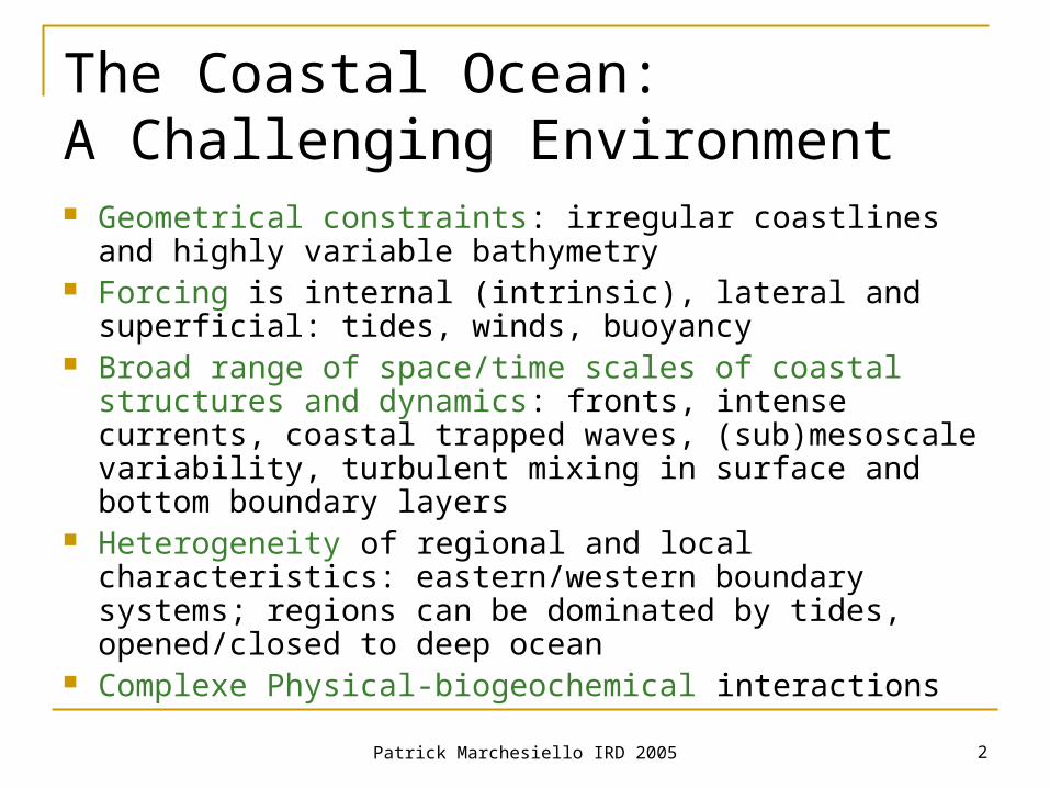
The Coastal Ocean: A Challenging Environment Geometrical constraints: irregular coastlines and highly
variable bathymetry Forcing is internal (intrinsic), lateral and superficial: tides,
winds, buoyancy Broad range of space/time scales of coastal structures
and dynamics: fronts, intense currents, coastal trapped waves, (sub)mesoscale variability, turbulent mixing in surface and bottom boundary layers
Heterogeneity of regional and local characteristics: eastern/western boundary systems; regions can be dominated by tides, opened/closed to deep ocean
Complexe Physical-biogeochemical interactions

Patrick Marchesiello IRD 2005 3
Numerical Modeling
Require highly optimized models of significant dynamical complexity
In the past: simplified models due to limited computer resources
In recent years: based on fully nonlinear stratified Primitive Equations
Patrick Marchesiello IRD 2005 4
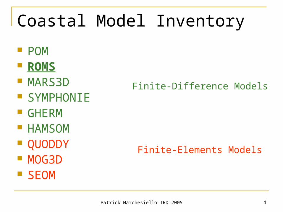
Coastal Model Inventory
POM ROMS MARS3D SYMPHONIE GHERM HAMSOM QUODDY MOG3D SEOM
Finite-Difference Models
Finite-Elements Models
Patrick Marchesiello IRD 2005 5

Patrick Marchesiello IRD 2005 6
Hydrodynamics
Patrick Marchesiello IRD 2005 7
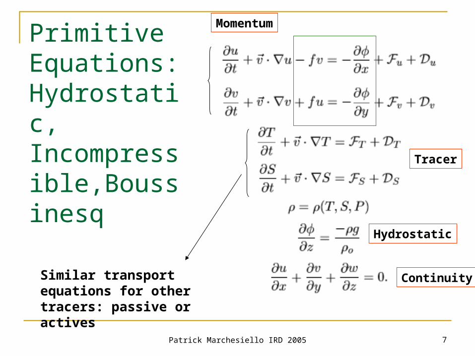
Primitive Equations:Hydrostatic, Incompressible,Boussinesq
Similar transport equations for other tracers: passive or actives
Hydrostatic
Continuity
Tracer
Momentum

Patrick Marchesiello IRD 2005 8
Vertical Coordinate System
Bottom following coordinate (sigma): best representation of bottom dynamics:
but subject to pressure gradient errors on steep bathymetry
Patrick Marchesiello IRD 2005 9
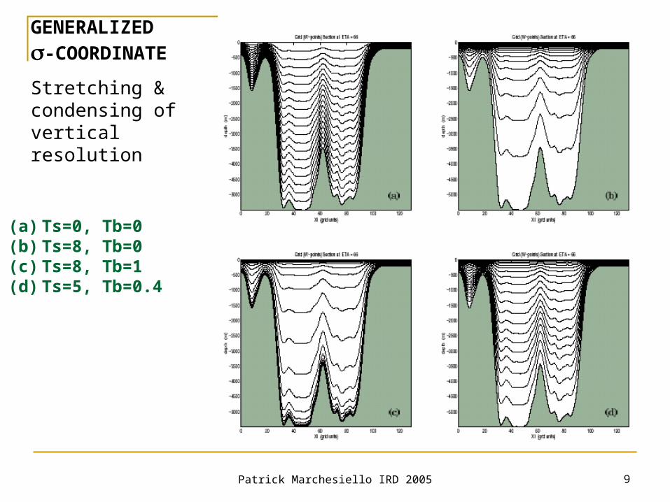
GENERALIZED
-COORDINATE
Stretching & condensing of vertical resolution
(a) Ts=0, Tb=0(b) Ts=8, Tb=0(c) Ts=8, Tb=1(d) Ts=5, Tb=0.4
Patrick Marchesiello IRD 2005 10
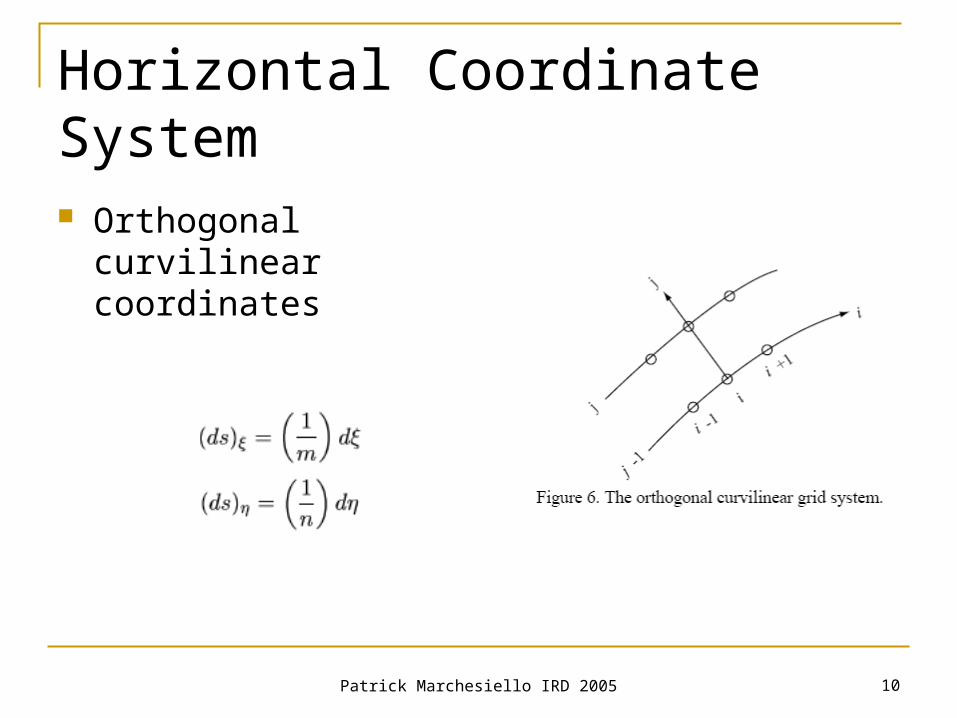
Horizontal Coordinate System Orthogonal curvilinear
coordinates
Patrick Marchesiello IRD 2005 11
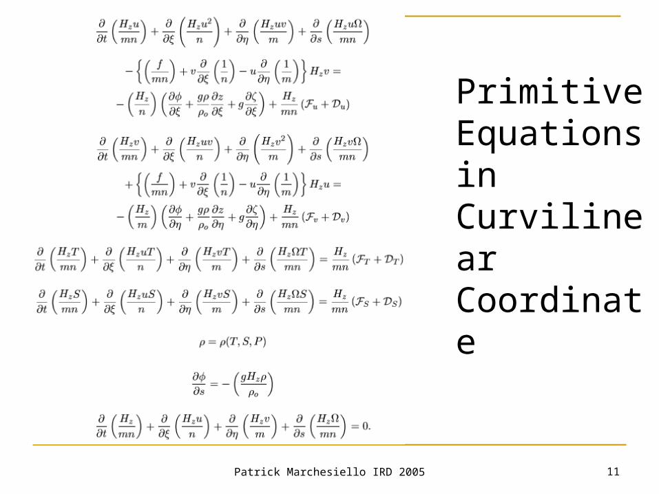
Primitive Equations in Curvilinear Coordinate
Patrick Marchesiello IRD 2005 12
Simplified Equations
2D barotropic Tidal problems
2D vertical Upwelling
1D vertical Turbulent mixing problems (with
boundary layer parameterization)

Patrick Marchesiello IRD 2005 13
Barotropic Equations
Patrick Marchesiello IRD 2005 14
Vertical Problems:Parameterization of Surface and Bottom Boundary Layers

Patrick Marchesiello IRD 2005 15
Boundary Layer Parameterization
Boundary layers are characterized by strong turbulent mixing
Turbulent Mixing depends on: Surface/bottom forcing:
Wind / bottom-shear stress stirring Stable/unstable buoyancy forcing
Interior conditions: Current shear instability Stratification
w’T’
Reynolds term:
K theory

Patrick Marchesiello IRD 2005 16
Surface and Bottom Forcing
Wind stress
Heat FluxSalt Flux
Bottom stress
Drag Coefficient CD:γ1=3.10-4 m/s Linearγ2=2.5 10-3 Quadratic

Patrick Marchesiello IRD 2005 17
Boundary Layer Parameterization All mixed layer schemes are based on
one-dimentional « column physics » Boundary layer parameterizations are
based either on: Turbulent closure (Mellor-Yamada, TKE) K profile (KPP)
Note: Hydrostatic stability may require large vertical diffusivities: implicit numerical methods are best suited. convective adjustment methods (infinite
diffusivity) for explicit methods

Patrick Marchesiello IRD 2005 18
Application: Tidal Fronts
ROMS Simulation in the Iroise Sea (Front d’Ouessant)
Simpson-Hunter Simpson-Hunter criterium for tidal criterium for tidal
fronts positionfronts position
1.5 < < 2
H. Muller, 2004
Patrick Marchesiello IRD 2005 19
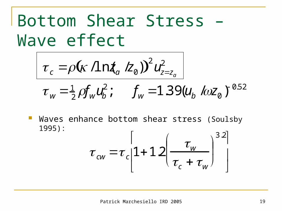
Bottom Shear Stress – Wave effect
c /ln(za /z0) 2uzza
2
w 12fwub
2; fw 1.39(ub /z0 ) 0.52
Waves enhance bottom shear stress (Soulsby 1995):
cw c 11.2w
c w
3.2
Patrick Marchesiello IRD 2005 20
Numerical Discretization

Patrick Marchesiello IRD 2005 21
A Discrete Ocean
Patrick Marchesiello IRD 2005 22
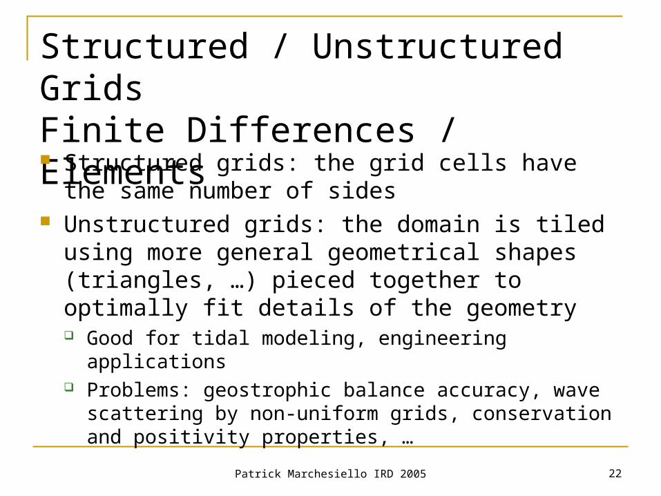
Structured / Unstructured GridsFinite Differences / Elements
Structured grids: the grid cells have the same number of sides
Unstructured grids: the domain is tiled using more general geometrical shapes (triangles, …) pieced together to optimally fit details of the geometry Good for tidal modeling, engineering applications Problems: geostrophic balance accuracy, wave scattering
by non-uniform grids, conservation and positivity properties, …

Patrick Marchesiello IRD 2005 23
Finite Difference (Grid Point) Method If we know:
The ocean state at time t (u,v,w,T,S, …) Boundary conditions (surface, bottom, lateral
sides) We can compute the ocean state at t+dt
using numerical approximations of Primitive Equations

Patrick Marchesiello IRD 2005 24
Horizontal and Vertical Grids
Patrick Marchesiello IRD 2005 25
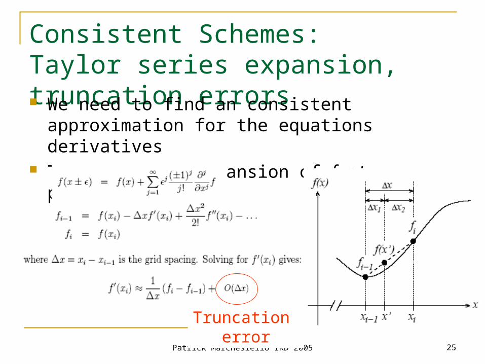
Consistent Schemes: Taylor series expansion, truncation errors We need to find an consistent approximation
for the equations derivatives Taylor series expansion of f at point x:
Truncation error

Patrick Marchesiello IRD 2005 26
Exemple: Advection Equation
x
t
x grid space
t time step

Patrick Marchesiello IRD 2005 27
Order of Accuracy
First order
2nd order
4th order
Downstream
Upstream
Centered

Patrick Marchesiello IRD 2005 28
Numerical properties: stability, dispersion/diffusion
Leapfrog / CenteredTi
n+1 = Ti n-1 - C (Ti+1n - Ti-1
n) ; C = u0 dt / dxConditionally stable: CFL condition C < 1 but dispersive (computational modes)
Euler / CenteredTi
n+1 = Ti n - C (Ti+1n - Ti-1
n)Unconditionally unstable
UpstreamTi
n+1 = Ti n - C (Tin - Ti-1
n) , C > 0Ti
n+1 = Ti n - C (Ti+1n - Ti
n) , C < 0Conditionally stable, not dispersive but diffusive
(monotone linear scheme)
Advection equation:
2nd order approx to the modified equation:
should be non-dispersive:the phase speed ω/k and group speed δω/δk are equal and constant (uo)

Patrick Marchesiello IRD 2005 29
Numerical Properties
A numerical scheme can be:
• Dispersive: ripples, overshoot and extrema (centered)
• Diffusive (upstream)
• Unstable (Euler/centered)

Patrick Marchesiello IRD 2005 30
Weakly Dispersive, Weakly Diffusive Schemes Using high order upstream schemes:
3rd order upstream biased Using a right combination of a centered scheme
and a diffusive upstream scheme TVD, FCT, QUICK, MPDATA, UTOPIA, PPM
Using flux limiters to build nolinear monotone schemes and guarantee positivity and monotonicity for tracers and avoid false extrema (FCT, TVD)
Note: order of accuracy does not reduce dispersion of shorter waves

Patrick Marchesiello IRD 2005 31
Upstream
Centered
2nd order flux limited
3rd order flux limited
Durran, 2004
Patrick Marchesiello IRD 2005 32
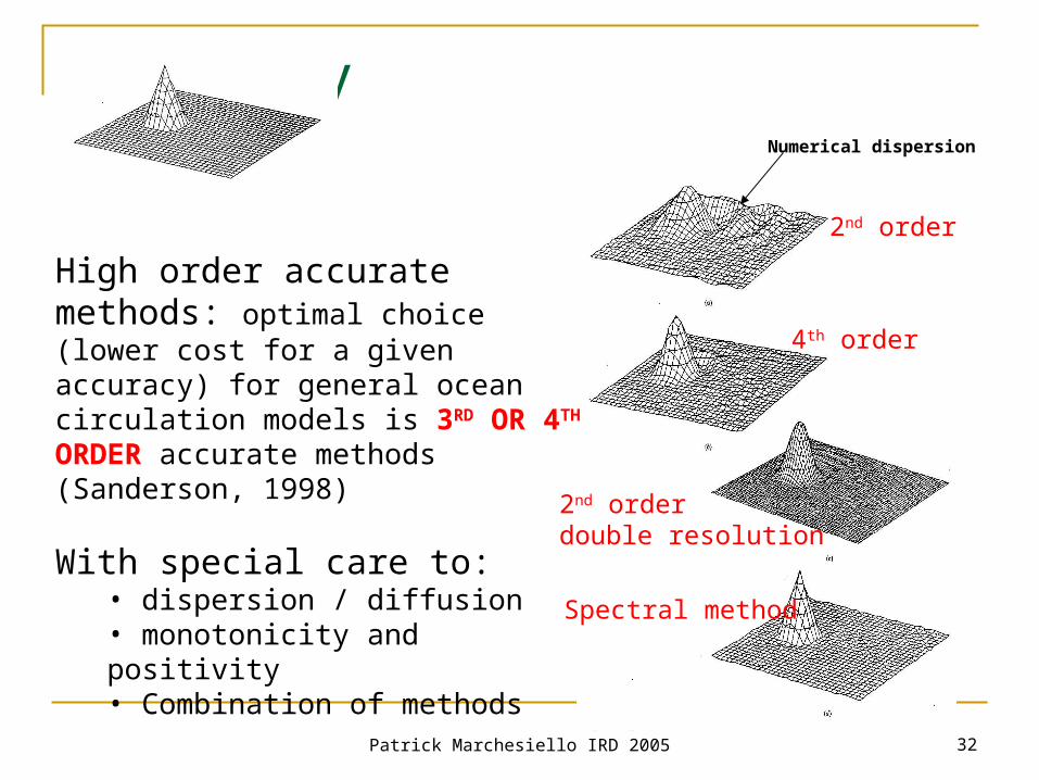
Accuracy
2nd order
4th order
2nd orderdouble resolution
Spectral method
Numerical dispersion
High order accurate methods: optimal choice (lower cost for a given accuracy) for general ocean circulation models is 3RD OR 4TH ORDER accurate methods (Sanderson, 1998)
With special care to:• dispersion / diffusion• monotonicity and positivity• Combination of methods
Patrick Marchesiello IRD 2005 33
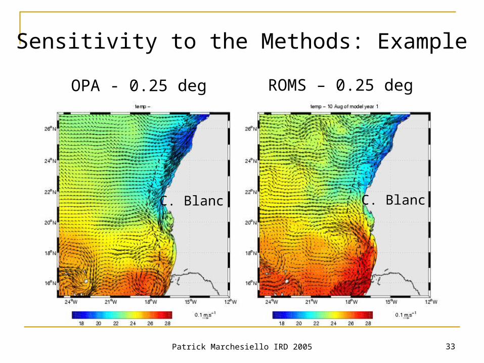
OPA - 0.25 deg ROMS – 0.25 deg
C. Blanc C. Blanc
Sensitivity to the Methods: Example
Patrick Marchesiello IRD 2005 34
Properties of Horizontal Grids

Patrick Marchesiello IRD 2005 35
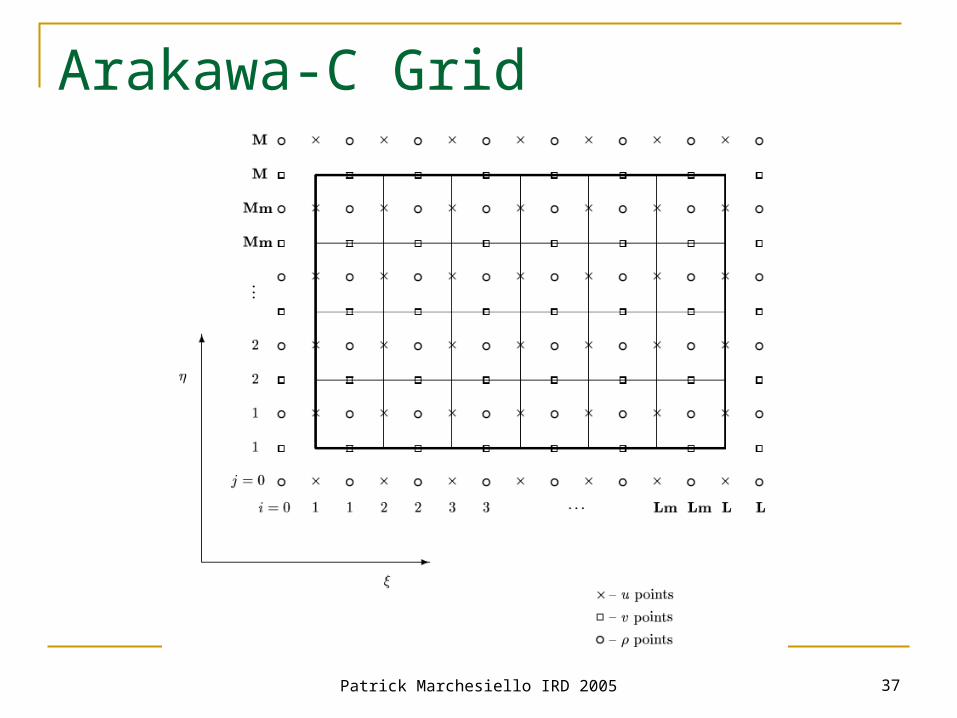
Arakawa Staggered GridsLinear shallow water equation:
A staggered difference is 4 times more accurate than non-staggered and improves the dispersion relation because of reduced use of averaging operators

Patrick Marchesiello IRD 2005 36
Horizontal Arakawa grids B grid is prefered at coarse resolution:
Superior for poorly resolved inertia-gravity waves. Good for Rossby waves: collocation of velocity points. Bad for gravity waves: computational checkboard mode.
C grid is prefered at fine resolution: Superior for gravity waves. Good for well resolved inertia-gravity waves. Bad for poorly resolved waves: Rossby waves
(computational checkboard mode) and inertia-gravity waves due to averaging the Coriolis force.
Combinations can also be used (A + C)
Patrick Marchesiello IRD 2005 37
Arakawa-C Grid

Patrick Marchesiello IRD 2005 38
Vertical Staggered Grid
Patrick Marchesiello IRD 2005 39
Numerical Round-off Errors
Patrick Marchesiello IRD 2005 40
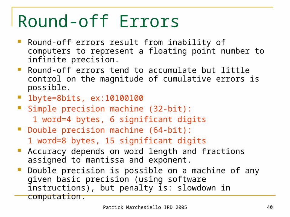
Round-off Errors Round-off errors result from inability of computers to represent a
floating point number to infinite precision. Round-off errors tend to accumulate but little control on the
magnitude of cumulative errors is possible. 1byte=8bits, ex:10100100 Simple precision machine (32-bit):
1 word=4 bytes, 6 significant digits Double precision machine (64-bit):
1 word=8 bytes, 15 significant digits Accuracy depends on word length and fractions assigned to
mantissa and exponent. Double precision is possible on a machine of any given basic
precision (using software instructions), but penalty is: slowdown in computation.

Patrick Marchesiello IRD 2005 41
Time Stepping

Patrick Marchesiello IRD 2005 42
Time Stepping: Standard
Leapfrog: φin+1 = φi n-1 + 2 Δt F(φi
n) computational mode amplifies when applied to
nonlinear equations (Burger, PE)
Leapfrog + Asselin-Robert filter:φi
n+1 = φfi n-1 + 2 Δt F(φin)
φfi n = φi n + 0.5 α (φin+1 - 2 φi
n + φfin-1)
reduction of accuracy to 1rst order depending on α (usually 0.1)

Patrick Marchesiello IRD 2005 43Kantha and Clayson (2000) after Durran (1991)
Time Stepping: Performance
C = 0.5 C = 0.2
Patrick Marchesiello IRD 2005 44
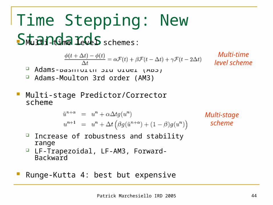
Time Stepping: New Standards Multi-time level schemes:
Adams-Bashforth 3rd order (AB3) Adams-Moulton 3rd order (AM3)
Multi-stage Predictor/Corrector scheme
Increase of robustness and stability range LF-Trapezoidal, LF-AM3, Forward-Backward
Runge-Kutta 4: best but expensive
Multi-time level scheme
Multi-stage scheme

Patrick Marchesiello IRD 2005 45
Barotropic Dynamicsand Time Splitting

Patrick Marchesiello IRD 2005 46
Time step restrictions The Courant-Friedrichs-Levy CFL stability condition on the
barotropic (external) fast mode limits the time step:
Δtext < Δx / Cext where Cext = √gH + Uemax
ex: H =4000 m, Cext = 200 m/s (700 km/h)
Δx = 1 km, Δtext < 5 s Baroclinic (internal) slow mode:
Cin ~ 2 m/s + Uimax (internal gravity wave phase speed + max advective velocity)
Δx = 1 km, Δtext < 8 mn
Δtin / Δtext ~ 60-100 ! Additional diffusion and rotational conditions:
Δtin < Δx2 / 2 Ah and Δtin < 1 / f

Patrick Marchesiello IRD 2005 47
Barotropic Dynamics The fastest mode (barotropic) imposes a
short time step 3 methods for releasing the time-step
constraint: Rigid-lid approximation Implicit time-stepping Explicit time-spitting of barotropic and baroclinic
modes Note: depth-averaged flow is an
approximation of the fast mode (exactly true only for gravity waves in a flat bottom ocean)

Patrick Marchesiello IRD 2005 48
Rigid-lid Streamfunction Method Advantage: fast mode is properly filtered Disadvantages:
Preclude direct incorporation of tidal processes, storm surges, surface gravity waves.
Elliptic problem to solve: convergence is difficult with complexe geometry; numerical
instabilities near regions of steep slope (smoothing required) Matrix inversion (expensive for large matrices); Bad
scaling properties on parallel machines Fresh water input difficult Distorts dispersion relation for Rossby waves

Patrick Marchesiello IRD 2005 49
Implicit Free Surface Method
Numerical damping to supress barotropic waves
Disadvantanges: Not really adapted to tidal processes unless Δt is
reduced, then optimality is lost Involves an elliptic problem
matrix inversion Bad parallelization performances

Patrick Marchesiello IRD 2005 50
Time SplittingExplicit free surface method
Patrick Marchesiello IRD 2005 51
Barotropic Dynamics:Time Splitting Direct integration of barotropic equations, only few
assumptions; competitive with previous methods at high resolution (avoid penalty on elliptic solver); good parallelization performances
Disadvantages: potential instability issues involving difficulty of cleanly separating fast and slow modes
Solution: time averaging over the barotropic sub-cycle finer mode coupling
Patrick Marchesiello IRD 2005 52
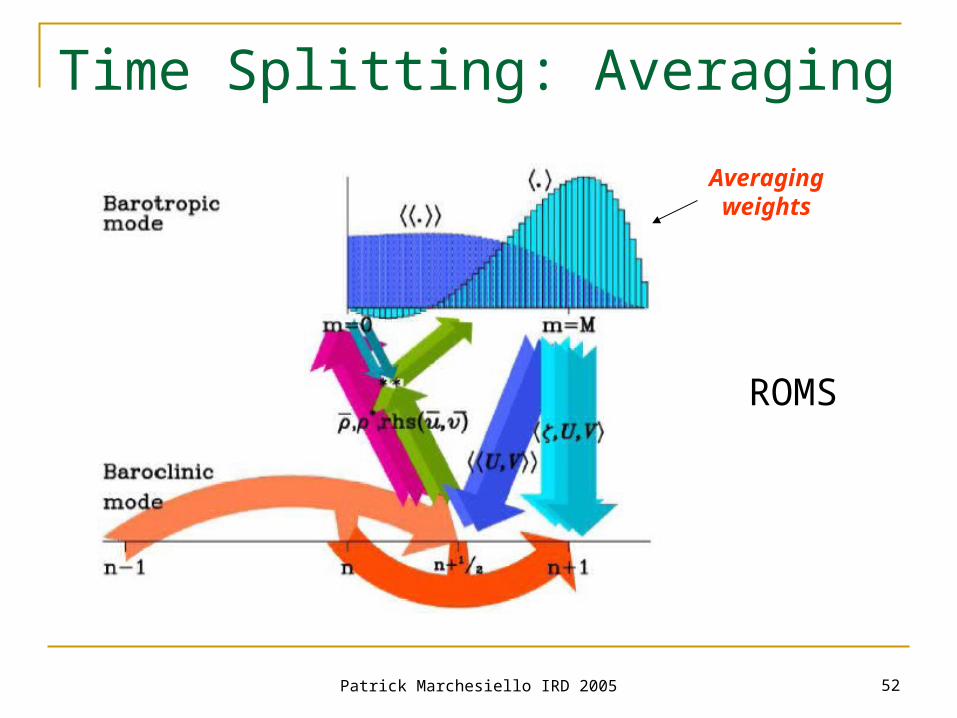
Time Splitting: Averaging
ROMS
Averaging weights
Patrick Marchesiello IRD 2005 53
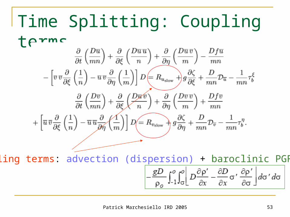
Time Splitting: Coupling terms
Coupling terms: advection (dispersion) + baroclinic PGF
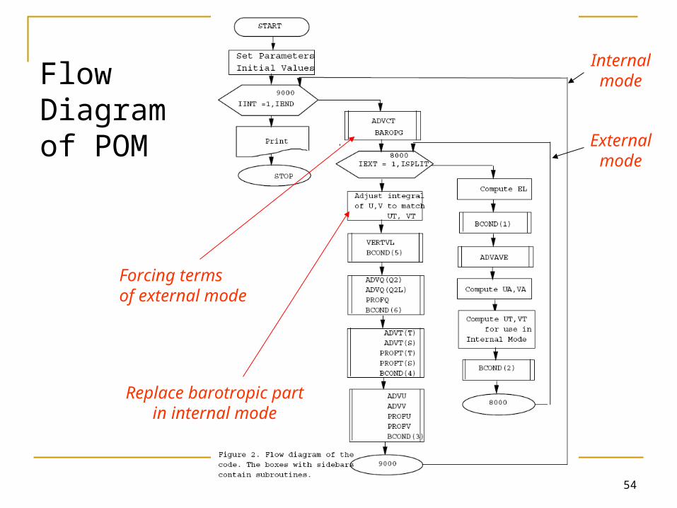
Patrick Marchesiello IRD 2005 54
Flow Diagram of POM External
mode
Internal mode
Forcing termsof external mode
Replace barotropic partin internal mode
Patrick Marchesiello IRD 2005 55
Vertical Diffusion

Patrick Marchesiello IRD 2005 56
Vertical Diffusion
Semi-implicitCrank-Nicholson scheme
Patrick Marchesiello IRD 2005 57
Pressure Gradient Force

Patrick Marchesiello IRD 2005 58
PGF Problem
Truncation errors are made from calculating the baroclinic pressure gradients across sharp topographic changes such as the continental slope
Difference between 2 large terms
Errors can appear in the unforced flat stratification experiment

Patrick Marchesiello IRD 2005 59
Reducing PGF Truncation Errors
Smoothing the topography using a nonlinear filter and a criterium:
Using a density formulation
Using high order schemes to reduce the truncation error (4th order, McCalpin, 1994)
Gary, 1973: substracting a reference horizontal averaged value from density (ρ’= ρ - ρa) before computing pressure gradient
Rewritting Equation of State: reduce passive compressibility effects on pressure gradient
r = Δh / h < 0.2
Patrick Marchesiello IRD 2005 60
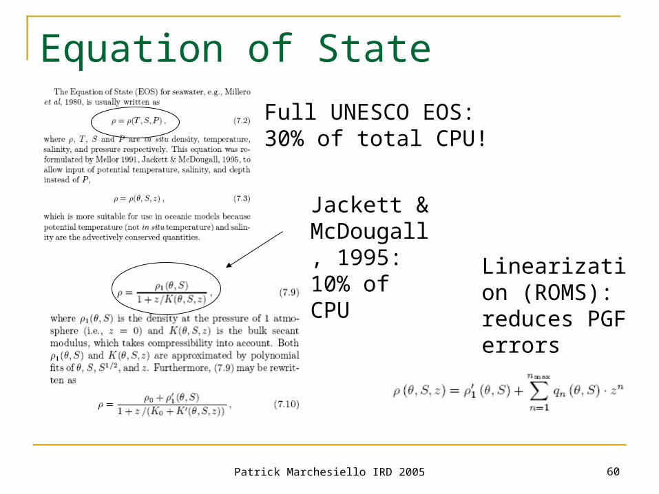
Equation of State
Jackett & McDougall, 1995: 10% of CPU
Full UNESCO EOS:30% of total CPU!
Linearization (ROMS): reduces PGF errors

Patrick Marchesiello IRD 2005 61
Smoothing methods
r = Δh / h is the slope of the logarithm of h One method (ROMS) consists of smoothing ln(h)
until r < rmax
Res: 5 kmr < 0.25
Res: 1 kmr < 0.25
Senegal Bathymetry Profil

Patrick Marchesiello IRD 2005 62
Smoothing method and resolution
Grid Resolution [deg]
Bathymetry Smoothing Error off Senegal
Convergence at ~ 4 km resolution
Sta
ndar
d D
evia
tion
[m]

Patrick Marchesiello IRD 2005 63
Errors in Bathymetry data compilations
Shelf errors(noise)
Etopo2: Satellite observationsGebco1 compilation

Patrick Marchesiello IRD 2005 64
Wetting and Drying Schemes
Patrick Marchesiello IRD 2005 65
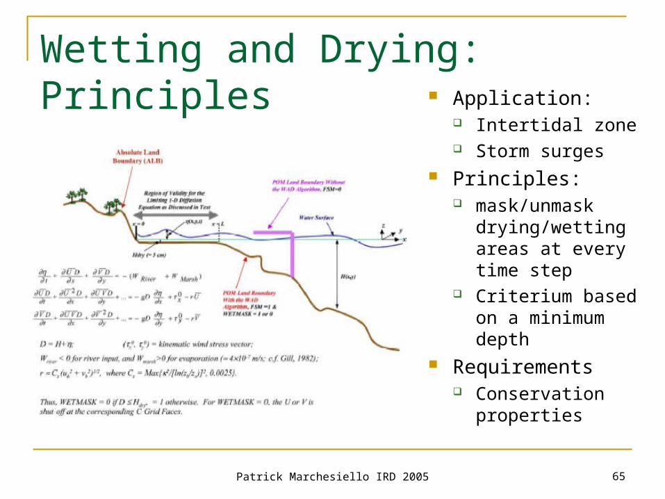
Wetting and Drying: Principles Application:
Intertidal zone Storm surges
Principles: mask/unmask
drying/wetting areas at every time step
Criterium based on a minimum depth
Requirements Conservation
properties