pathways calculus - calculus videos project · successful in calculus and future mathematics,...

FirstEdition

StudentWorkbook

MichaelA.TallmanMarilynP.CarlsonJamesHart

PATHWAYS through

CALCULUS AProblemSolvingApproach

i

Pathways Through Calculus

Student Workbook

First Edition

Michael A. Tallman Oklahoma State University

Marilyn P. Carlson

Arizona State University

James Hart Middle State Tennessee State University

Phoenix

ii

Introduction

Overview of Workbook Content This workbook contains investigations that we designed to help you build your own understanding of the central ideas of calculus. Many, but not all, of the investigations are accompanied by homework problems. We have intentionally included homework problems in that are much like problems in the investigations. This is so you can develop the thinking and understandings that will be needed to be successful in calculus and future mathematics, science, and engineering courses. The first two investigations review average and constant rate of change as well as linearity. These are essential prerequisite concepts for calculus. Investigation 3 explores the idea of local linearity, an important concept that underlies the notion of a derivative function, the main idea of Calculus I. Investigations 4–6 carefully develop your understanding of derivative functions by leveraging the meanings emphasized in Investigations 1–3. Investigation 7 introduces a method for computing the derivative of composite functions, again by leveraging the understandings developed in Investigations 1 and 2. Investigations 8 and 9 require you to apply your understanding of derivatives to solve novel problems. Finally, Investigation 10 introduces the notion of an accumulation function. By engaging with the questions in the investigations and homework, your reasoning and problem-solving abilities will get better and better. Over time you will become a powerful mathematical thinker who has confidence in your ability to solve novel problems on your own.

iii

To: The Calculus Student

Welcome! You are about to begin a new mathematical journey that we hope will lead to your choosing to continue to study mathematics. Even if you do not currently view yourself as being particularly talented at mathematics, it is very likely that these materials and this course will change your perspective. The materials in this workbook were designed with student learning and success in mind and are based on decades of research on mathematics teaching and learning. In addition to becoming more confident in your mathematical abilities, the reasoning patterns, problem solving abilities, and content knowledge you acquire will make more advanced courses in mathematics, the sciences, engineering, nursing, and business more accessible. The investigations will help you see a purpose for learning and understanding the ideas of calculus, while also helping you acquire critical knowledge and ways of thinking that will support your learning in future mathematics, science, and engineering courses. To assure your success, we ask that you make a strong effort to make sense of the questions you encounter. This will assure that your mathematical journey through this course is rewarding and transformational. Wishing you much success! Dr. Michael A. Tallman, Dr. Marilyn P. Carlson, Dr. James Hart

iv

Table of Contents___________________________________ Investigation 1. Constant Rate of Change and Linearity .........................................................................1 The focus of this investigation is on building students’ intuitive understanding of constant rate of change. By the end of the investigation we want students to understand that if the measure of one quantity varies at a constant rate with respect to the measure of another, then the changes in the measures of the quantities are proportional. Investigation 2. Average Rate of Change and the Difference Quotient ..................................................11 This investigation introduces students to the concept of average rate of change by connecting it to what they learned about constant rate of change in the previous investigation. We support students’ understanding of an average rate of change as the constant rate of change needed to change a specific amount in the output quantity for a specific amount of change in the input quantity. Investigation 3. Introduction to Local Linearity .......................................................................................22 The primary purpose of this investigation is to allow students to recognize that we often make the assumption that there is a roughly linear relationship between the input and output quantities of a function on small intervals of the domain. In other words, we often assume that the output quantity varies at a constant rate with respect to the input quantity over small intervals of the input quantity. This concept of local constant rate of change provides the conceptual foundation for the idea of derivative. Investigation 4. Introduction to Derivative ................................................................................................28 This investigation asks students to approximate the local constant rate of change of one quantity with respect to another at a specific value. We support students’ informal and intuitive understanding of a limiting process by asking them to compute average rates of change over increasingly smaller intervals. We also support students’ understanding of the slope of the line tangent to the graph of a function at a specific point as a geometric interpretation of the limiting value of average rates of change. Investigation 5. Instantaneous Rate of Change .........................................................................................42 This investigation supports students’ understanding of derivative at a point as the limiting value of a multiplicative comparison of the changes in quantities’ values, not a property of a geometric object like, “slope of the tangent line.” We emphasize the idea that “instantaneous rate of change” is a theoretical construct; for a rate of change to exist, there must be changes in quantities’ values to multiplicatively compare. Investigation 6. Derivative Function ..........................................................................................................54 The purpose of this investigation is to examine how the derivative function is generated and to understand the information it conveys. We leverage the meanings developed in previous investigations by continuously asking students to interpret symbolic and graphical representations of derivative functions in terms of rates of change. Investigation 7. Chain Rule .........................................................................................................................61 This investigation begins by providing students with an opportunity to review the graphical interpretation of function composition. Students then represent the average rate of change of various composite functions. This provides a conceptual foundation for the chain rule. The investigation concludes with a formalization of students’ representation of the average rate of change of the generic composite function (f o g)(x) with respect to x. This formalization, which results from applying a limit, results in the chain rule.

v

Investigation 8. Optimization ......................................................................................................................68 This investigating begins by supporting students’ understanding that the critical points of a differentiable function occur at input values for which the derivative equals zero. Students then apply this understanding to determine the maximum or minimum value of some quantity, provided particular constraints. Investigation 9. Related Rates .....................................................................................................................77 This investigation begins by introducing students to the notion of a related rate formula. Early tasks ask students to define formulas that express the relationship between two rates of change. Subsequent tasks require students to define a related rate formula and solve it to determine the rate of change of one quantity with respect to another. Investigation 10. Accumulation Functions .................................................................................................84 The objective of this investigation is to intuitively generate accumulation functions graphically and then capture this intuitive process into appropriate mathematical notation. At the conclusion of this investigation, students will have constructed a symbolic function rule that represents the accumulation of some quantity that is expressed in terms of how that quantity varies relative to some independent quantity.

Calculus Investigation 1 Constant Rate of Change and Linearity


© 2016 Tallman, Carlson, and Hart

1

1. Suppose Kim is riding her bike along a straight road at a constant rate of 0.56 km/min. Kim passes a

coffee shop while traveling at this constant rate. At 9:30 AM, Kim is 3 km past the coffee shop. a. How far is Kim from the coffee shop at 9:31 AM? b. How far is Kim from the coffee shop at 10:17 AM? c. How far is Kim from the coffee shop 24.6 minutes past 9:30 AM? d. Define a function that relates Kim’s distance from the coffee shop (in kilometers) in terms of the

number of minutes elapsed since Kim was 3 km past the coffee shop. Be sure to define your variables.

e. Let ∆t represent a change in the number of minutes elapsed while Kim is riding her bike at a

constant rate and let ∆d represent the corresponding change in the number of kilometers Kim traveled. How are ∆t and ∆d related? Write an equation that expresses the relationship between ∆t and ∆d.

f. Use your response to Part (e) to determine what time Kim passed the coffee shop.




2

g. Sketch a graph of the relationship between Kim’s distance from the coffee shop (in kilometers) and the number of minutes elapsed since Kim was 3 km past the coffee shop. Be sure to label your axes.

2. John Paul is driving on Interstate 35 from Norman, OK to Stillwater, OK. John Paul’s car consumes

fuel at a constant rate while he drives on I-35. The graph below represents the relationship between the number of miles John Paul has driven on I-35 (represented by the variable d) and the number of gallons of fuel his car has consumed since he started driving on I-35 (represented by the variable g). The point (70, 2.5) is on the graph, as indicated.

35

30

25

20

15

10

5

–5

10 20 30 40 50

3.5

3

2.5

2

1.5

1

0.5

–0.5

g

20 40 60 80d

(70, 2.5)




3

a. As the number of miles that John Paul has driven on I-35 changes from 0 to 12 miles, how much does the amount of fuel his car has consumed change? Represent this change on the graph and explain how you determined this change.

b. As the number of miles that John Paul has driven on I-35 changes from 21 to 27 miles, how much

does the amount of fuel his car has consumed change? Represent this change on the graph and explain how you determined this change.

c. As the number of miles that John Paul has driven on I-35 changes from 56 to 62 miles, how much

does the amount of fuel his car has consumed change? Represent this change on the graph and explain how you determined this change.

d. How much does the amount of fuel John Paul’s car consumed change for any change of 6 miles

he has driven on I-35? e. As the number of miles that John Paul has driven on I-35 changes from d1 to d2 miles, how much

does the amount of fuel his car has consumed change? Explain how you determined this change.




4

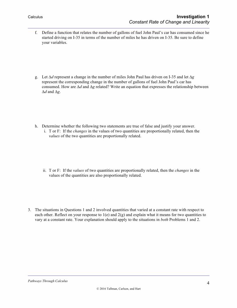
f. Define a function that relates the number of gallons of fuel John Paul’s car has consumed since he started driving on I-35 in terms of the number of miles he has driven on I-35. Be sure to define your variables.

g. Let ∆d represent a change in the number of miles John Paul has driven on I-35 and let ∆g

represent the corresponding change in the number of gallons of fuel John Paul’s car has consumed. How are ∆d and ∆g related? Write an equation that expresses the relationship between ∆d and ∆g.

h. Determine whether the following two statements are true of false and justify your answer.

i. T or F: If the changes in the values of two quantities are proportionally related, then the values of the two quantities are proportionally related.

ii. T or F: If the values of two quantities are proportionally related, then the changes in the

values of the quantities are also proportionally related.

3. The situations in Questions 1 and 2 involved quantities that varied at a constant rate with respect to each other. Reflect on your response to 1(e) and 2(g) and explain what it means for two quantities to vary at a constant rate. Your explanation should apply to the situations in both Problems 1 and 2.




5

4. Suppose Quantity A varies at a constant rate of –3.1 with respect to Quantity B. Let y represent the measure of Quantity A and let x represent the measure of Quantity B. When x has a value of 1.7, y has a value of 2.4. Use the meaning of constant rate of change you described in response to Question 3 to answer the following. a. Determine the change in the value of y as x changes by 1.9.

b. Determine the change in the value of x as y changes by –5.2.

c. Determine the value of y when x = 0.

d. Determine the value of x when y = 4.8.

5. Suppose Quantity A varies at a constant rate of m with respect to Quantity B. Let y represent the

measure of Quantity A and let x represent the measure of Quantity B. When x has a value of x1, y has a value of y1. Use the meaning of constant rate of change you described in response to Question 3 to answer the following. a. Determine the change in the value of y as x changes by ∆x. b. Determine the value of y when x = 0. c. Determine the value of y when x = 7.4. d. Write an equation that determines the value of y for any value of x.




6

Two quantities change at a constant rate with respect to each other if changes in one quantity are proportional to corresponding changes in the other. For example, suppose Quantity A changes at a constant rate with respect to Quantity B. If y represents the measure of Quantity A and x represents the measure of Quantity B, then the change in y is proportionally related to the change in x. This means that for any change in x, the corresponding change in y is always the same number of times as large. If we let m denote the number of times larger ∆y is than ∆x, we can express the proportional relationship between changes in the measures of Quantity A and Quantity B as ∆y = m∆x. The value of m is called the constant rate of change of Quantity A with respect to Quantity B. 6. Give three examples of pairs of quantities that vary at a constant rate with respect to each other.

Explain why each pair of quantities are related by a constant rate of change. 7. Suppose x and y represent the measures of two quantities that vary at a constant rate with respect to

each other. For Parts (a) – (c) below, use the given information to write a formula that defines the relationship between x and y. a. y changes at a constant rate of –0.9 with respect to x.

y = 2.4 when x = –5.8. b. y = 3.6 when x = 12.2.

y = –1.5 when x = 8.7. c.

3

2

1

–1

–2

–3

y

–4 –2 2 4

x




7

8. Suppose x and y represent the measures of two quantities that vary at a constant rate with respect to each other. For Parts (a) and (b) below, use the given information to write a formula that defines the relationship between x and y. a. y changes at a constant rate of m with respect to x.

y = y1 when x = x1.

b. y = y1 when x = x1.

y = y2 when x = x2.

Homework 1. What does it mean for an object to move at a constant speed? (Note: Please say something more than

“The speed doesn’t change.” Be descriptive and reference specific quantities.) 2. Paul was walking in a park. Assume that he walked at a constant speed during the entire trip, and also

suppose that during one part of the trip he walked 52.8 feet in 8 seconds. a. Provide at least four conclusions we can draw from the given information. b. How far did Paul walk in 14 seconds? c. Does your answer to Part (b) depend on which 14-second interval we’re talking about? Explain. d. How long did it take Paul to travel any 20-foot distance during his walk?

3. Suppose we have a partially filled pitcher of water and that we want to add more water to the pitcher.

We know that adding 60 ounces of water to the pitcher will increase the height of water in the pitcher by 7.8 inches, and that these two quantities are related by a constant rate of change. Define variables to represent the quantities in this context and then represent the relationship between corresponding changes in these quantities.

4. Suppose we know that ∆y = m·∆x for some constant m, and we are given the information in the

following table. What is the value of m? x y

–3 15.5 1 5.5 3 0.5 8 –12




8

5. Suppose we know that ∆y = m·∆x for some constant m, and we are given the information in the following graph. What is the value of m?

6. Suppose we know that the changes in the values of two variables are related according to ∆y = 3·∆x.

a. If we start off at x = 5 and let x change to be x = 12, i. What is the change in x?

ii. By how much does y change for the change in x you found in Part (i)? iii. Suppose we know that y = –2 when x = 5. What is the value of y when x = 12? How did you

find this? b. If we start off at x = 7 and let x change to be x = –3,

i. What is the change in x? ii. By how much does y change for the change in x you found in Part (i)?

iii. Suppose we know that y = 8 when x = 7. What is the value of y when x = –3? How did you find this?

7. Suppose you have a cell phone plan whose cost is based on the number of minutes you talk. Let n

represent the number of minutes talked in a month and let c represent the monthly cost of using your phone (in dollars). Furthermore, suppose c = 45.70 when n = 95 and that ∆c = 0.06·∆n. a. What is the value of c when n = 325? What does this tell us? b. What is the value of c when n = 0? What does this tell us?

8. Suppose we are given that ∆y = 4.5·∆x and that when x = 1, y = 4. We want to know the new value of

y when x = –4 . Answer the questions that follow. y = 4.5(x – 1) + 4 y = 4.5(–4 – 1) + 4 a. What does –4 – 1 represent? y = 4.5(–5) + 4 b. What does 4.5(–5) represent? y = –22.5 + 4 c. What does –22.5 + 4 represent? y = –18.5 d. What does –18.5 represent?

9. The constant rate of change of y with respect to x is 4, and (5, 4) is a point on the graph.

a. Write the formula for the linear function. b. Find the value of y when x = 2.




9

10. The constant rate of change of y with respect to x is –3.2, and (–3, –2) is a point on the graph.

a. Write the formula for the linear function. b. Find the value of y when x = 5.

11. Write the formula for each of the linear functions described below. a. y changes at a constant rate of 4.8 with respect to x, and (7, 9.3) is a point on the graph. b. y changes at a constant rate of –1.9 with respect to x, and (4, 6) is a point on the graph. 12. Write the formula that defines the linear relationship represented in each of the following graphs.

a. b.

13. Write the formula that defines the linear relationship represented in each of the following graphs.

a. b.




10

14. Write the formula that defines the linear relationship given in each of the following tables. a. b.

x y w d –6 16 –9 0 –1 1 –4 10 2 –8 1 20 8 –26 14 46

15. Write the formula that defines the linear relationship given in each of the following tables.

a. b. x y w d

–5 –15.5 –12 17.5 –1 –1.5 –8 11.5 2 9 3 –5

18 65 17 –26

Calculus Investigation 2 Average Rate of Change and the Difference Quotient



11

1. A car is driving away from a crosswalk. The distance d (in feet) of the car from the crosswalk t

seconds since the car started moving is given by the formula d = t2 + 3.5. a. Does the car’s distance (in feet) from the crosswalk vary at a constant rate with respect to the

number of seconds elapsed since the car started moving? Justify your response using the meaning of constant rate of change.

b. A second car traveling at a constant rate passed the first car the moment it started moving (at t =

0). The first car passed the second car 17 seconds later. i. At what constant speed was the second car traveling? ii. Below is a graph of the relationship between the first car’s distance d (in feet) from the

crosswalk and the number of seconds t elapsed since the car started moving. Illustrate on this graph the constant speed of the second car computed in Part (i) from t = 0 to t = 17. Explain how what you drew illustrates the second car’s constant rate of change.

300

250

200

150

100

50

d

5 10 15t




12

2. A car is driving through an intersection after having stopped at a red light. The distance d (in feet) of the car north of the intersection t seconds after it started moving is given by the formula d = 2t2 – 4. a. Does the car’s distance (in feet) north the intersection vary at a constant rate with respect to the

number of seconds elapsed since the car started moving? Justify your response using the meaning of constant rate of change.

b. A second car traveling at a constant rate passed the first car 3 seconds after it started moving. The

first car passed the second car 11.5 seconds after the first car started moving. i. At what constant speed was the second car traveling? ii. Below is a graph of the relationship between the first car’s distance d (in feet) north of the

intersection and the number of seconds t elapsed since the car started moving. Illustrate on this graph the constant speed of the second car computed in Part (i) from t = 3 to t = 11.5. Explain how what you drew illustrates the second car’s constant rate of change.

250

200

150

100

50

d

2 4 6 8 10 12t




13

3. While running a road race, Alima’s distance d (in miles) from the start line t minutes after she passed the start line is given by the formula d = 0.3t0.7. a. Does Alima’s distance (in miles) from the start line vary at a constant rate with respect to the

number of minutes elapsed since she passed the start line? Justify your response using the meaning of constant rate of change.

b. Six minutes after Alima passed the start line, she passed Miguel who was running at a constant

speed. Eight minutes later, Miguel passed Alima. i. At what constant speed was Miguel running? ii. Below is a graph of the relationship between Alima’s distance d (in miles) from the start line

and the number of minutes t elapsed since she passed the start line. Illustrate on this graph Miguel’s constant speed you computed in Part (i) from t = 6 to t = 14. Explain how what you drew illustrates Miguel’s constant speed.

3

2.5

2

1.5

1

0.5

d

5 10 15t




14

4. Let f(x) = –x2 + 7. a. Does f(x) vary at a constant rate with respect to x? Justify your response using the meaning of

constant rate of change. b. i. What is the constant rate of change of the linear function g that has the same change in output

values over the interval x = –3 to x = 5 as the function f? ii. Below is a graph of f. Illustrate on this graph the constant rate of change you computed in

Part (i) from x = –3 to x = 5. Explain how what you drew illustrates a constant rate of change.

In Part (b) of Problems 1-4, you computed what is called an average rate of change. The average rate of change of a function f from x = x1 to x = x2 is the constant rate of change of a linear function g that has the same change in output as the function f over the interval [x1, x2]. The function g has the same change in output as the function f from x = x1 to x = x2 if f(x1) = g(x1) and f(x2) = g(x2). The average rate of change of f over the interval [x1, x2] is the constant rate of change

g(x2 )− g(x1)x2 − x1

of the linear function g.

20

10

–10

–20

f(x)

–4 –2 2 4 6

x




15

5. Use the definition of average rate of change above to explain why the values you computed in response to Part (b) of Problems 1-4 are average rates of change.

6. Write an expression that represents the average rate of change of the function f over the interval

[x1, x2].

7. An open-top box is created by cutting squares out of the corners of an 8.5-inch by 11-inch sheet of

paper and then folding up the sides (see image below).

a. Define a function f to determine the volume of the box (measured in cubic inches) in terms of the length x of the side of the square cutout (in inches).

b. Describe the meaning of each of the following expressions in the context of the situation:

i. f(x + 3) ii. f(x + 3) – f(x) iii. ( 3) ( )( 3)

f x f xx x+ −+ −

c. Evaluate ( 3) ( )

( 3)f x f xx x+ −+ − for x = 0.5. Describe the meaning of this value in the context of the situation.




16

8. The area A (measured in square feet) of a circular oil slick as a function of the amount of time (measured in minutes) since the oil leak started is given by the function g(t) = π(7.84t)2. a. Describe the meaning of ( 5) ( )

5g t g t+ − (simplified from ( 5) ( )

( 5)g t g tt t+ −+ − ) in the context of this situation.

b. Evaluate ( 5) ( )

5g t g t+ − when t = 1.5. Describe the meaning of this value.

In general, the expression ( ) ( )f x h f xh

+ − (simplified from ( ) ( )( )

f x h f xx h x+ −+ − ) where h represents the change in x is

called the difference quotient. The difference quotient is the average rate of change for a function between two input-output pairs (see Point A to Point B on the graph below). Using function notation, we say that you can find the average rate of change between any two points (x, f(x)) and (x + h, f(x + h)) by computing:

Δf ( x )Δx = f ( x+h)− f ( x )

( x+h)−x = f ( x+h)− f ( x )h . Thus, when computing the difference quotient for two points on

a function, you are determining the average rate of change between those two input-output pairs.

9. The function j defined by the formula j(t) = 1,645(1.06)t determines the population of Telluride,

Colorado t years since January 1, 1990. Define a function g that determines the average rate of change of Telluride’s population over any 0.2-year interval since January 1, 1990.

x

y

y = f(x)

x x+h

A

B




17

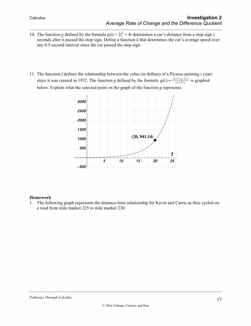
10. The function g defined by the formula g(t) = 2t2 + 4t determines a car’s distance from a stop sign t seconds after it passed the stop sign. Define a function k that determines the car’s average speed over any 0.5-second interval since the car passed the stop sign.

11. The function f defines the relationship between the value (in dollars) of a Picasso painting t years

since it was created in 1932. The function g defined by the formula g(t) = f (t+1.2)− f (t )(t+1.2)−t is graphed

below. Explain what the selected point on the graph of the function g represents.

Homework 1. The following graph represents the distance-time relationship for Kevin and Carrie as they cycled on

a road from mile marker 225 to mile marker 230.

3000

2500

2000

1500

1000

500

–5005 10 15 20 25

t

(20, 941.14)




18

a. How does the distance traveled and time elapsed compare for Carrie and Kevin as they traveled

from mile marker 225 to mile marker 230? b. How do Carrie and Kevin’s speeds compare as they travel from mile marker 225 to mile marker

230? c. How do Carrie and Kevin’s average speeds compare over the time interval as they traveled from

mile marker 225 to mile marker 230?

2. When running a marathon you heard the timer call out 12 minutes as you passed mile-marker 2. a. What quantities could you measure to determine your speed as you ran the race? Define variables

to represent the quantities’ values and state the units you will use to measure the value of each of these quantities.

b. As you passed mile-marker 5 you heard the timer call out 33 minutes. What was your average speed from mile 2 to mile 5?

c. Assume that you continued running at the same constant speed as computed in Part (b) above. How much distance did you cover as your time spent running increased from 35 minutes after the start of the race to 40 minutes after the start of the race?

d. If you passed mile marker 5 at 33 minutes, what average speed do you need to run for the remainder of the race to meet your goal to complete the 26.2-mile marathon in 175 minutes?

e. What is the meaning of average speed in this context? 3. On a trip from Tucson to Phoenix via Interstate 10, you used your cruise control to travel at a constant

speed for the entire trip. Since your speedometer was broken, you decided to use your watch and the mile markers to determine your speed. At mile marker 219 you noticed that the time on your digital watch just advanced to 9:22 AM. At mile marker 197 your digital watch advanced to 9:46 AM. a. Compute the constant speed at which you traveled over the time period from 9:22 AM to 9:46

AM. b. As you were passing mile marker 219 you also passed a truck. The same truck sped by you at

exactly mile marker 197. i. Construct a distance-time graph of your car. On the same graph, construct one possible

distance-time graph for the truck. Be sure to label the axes.

Time elapsed (in minutes) since passing mile marker 2252 4 6 8 12

Dis

tanc

e tra

vele

d (in

mile

s) s

ince

pas

sing

m

ile m

arke

r 225

1

2

3

4

5

14 16 18

Kevin’s Dista

nce-Time R

elationship

Carrie’s

Distance-

Time Relat

ionship




19

ii. Compare the speed of the truck to the speed of the car between 9:22 AM and 9:45 AM. iii. Compare the distance that your car traveled over this part of the trip with the distance that the

truck traveled over this same part of the trip. Compare the time that it took the truck to travel this distance with the time that it took your car to travel this distance. What do you notice?

iv. Why are the average speed of the car and the average speed of the truck the same? v. Phoenix is another 53 miles past mile marker 197. Assuming you continued at the constant

speed, at what time should you arrive in Phoenix?

4. The graph that follows represents the speeds of two cars (Car A and Car B) in terms of the elapsed time in seconds since being at a rest stop. Car A is traveling at a constant speed of 62 miles per hour. As Car A passes the rest stop, Car B pulls out beside Car A and they both continue traveling down the highway.

a. Which graph represents Car A’s speed and which graph represents Car B’s speed? Explain. b. Which car is further down the road 20 seconds after being at the rest stop? Explain. c. Explain the meaning of the intersection point. d. What is the relationship between the positions of Car A and Car B 27 seconds after being at the

rest stop? e. Car B catches up with Car A 64.5 seconds after Car A and Car B passed the rest stop. What is the

average speed of Car B over the interval from 0 seconds to 64.5 seconds after leaving the rest stop? Explain.

Instructions for Problems 5-14: Let d be the distance of a car (in feet) from mile marker 420 on a country road and let t be the time elapsed (in seconds) since the car passed mile marker 420. The formulas below represent various ways these quantities might be related. For each of the following:

i. Determine the average speed of the car using the given formula and the specified time interval. ii. Explain the meaning of average speed in the context of this situation.

5. d = t2 from t = 5 to t = 30. 6. d = –3(–19t – 1) from t = 3 to t = 9.

Time elapsed (in seconds) since passing rest stop10 20 30 40 50

Spee

d of

the

car (

in m

iles

per h

our)

20

40

60

80

100




20

7. d = 5(12t + 1) + 3t from t = 0.5 to t = 3.75. 8. 10 ( 5) 14

2t td + −= from t = 0 to t = 5.

9. ( )21

3 9 155 (11 6)d t t t= + − − from t = 2 to t = 4.

10. d = (2t + 7)(3t – 2) from t = 2 to t = 2.75. 11. ( )( )1 1

3 260d t t= + + from t = 1 to t = 4. 12. 27

8( 6)( 3) 7 20 11d t t t t t= + + + − + − from t = 30 to t = 35. 13. ( )21

8 3 1.5 16 3d t t t t= + + − from t = 2 to t = 4.

14. ( ) ( )2 21 1 42 10 315 3

5tt t t t

d+ + +

= from t = 5 to t = 9.

15. Consider the function f defined by f(x) = x2 – 6x + 10 that represents the altitude of a U.S. Air Force

test plane (in thousands of feet) during a recent test flight as a function of elapsed time (in minutes) since being released from its airborne launcher. a. Find the average rate of change of the plane’s altitude with respect to time as the time varies from

x = 2 minutes to x = 2.1 minutes. Show your work. b. What is the meaning of the average rate of change you determined in Part (a) in this context? c. Explain the meaning of the expression f(k + 0.1). d. Explain the meaning of the expression f(k + 0.1) – f(k).

f. What does the expression f (k + 0.1)− f (k)k + 0.1( )− k represent in the context of this problem?

16. Write an expression that represents the average rate of change of the given function over an input

interval of length h. Be sure to simplify your answer. a. f(x) = 12x + 6.5 b. f(x) = 97 c. f(x) = 6x2 + 7x – 11 d. f(x) = 3x3 – 9

e. f (x) = 12x




21

17. Use the graph of y = f(x) and an input value of x = k to represent the following quantities on the graph. a. f(k) b. k + 2.5 c. f(k + 2.5) d. f(k + 2.5) – f(k)

e. Represent the quantity f (k+2.5)− f (k )

2.5 on the graph above. Explain how what you drew represents the

value of this quantity.

10

8

6

4

2

–2

y

2 4 6 8

x

y = f(x)

Calculus Investigation 3 Introduction to Local Linearity



22

The understandings promoted in this investigation were informed by the content in Chapter 4 of Calculus: Newton Meets Technology by Patrick Thompson, Mark Ashbrook, Stacy Musgrave, and Fabio Milner (Thompson et al., 2015). 1. A stone is dropped into a lake creating a circular ripple that travels outward.

a. Define a function f that determines the area f(r) of a circle (in square inches) in terms of the circle’s radius length r (in inches).

b. Construct a graph of f on the given axes.

c. Does the area of a circle increase at a constant rate of change with respect to its radius length? Explain.

d. Use f to determine the average rate of change of the area of the circle (with respect to the radius)

as r changes from: i. 1.5 to 2 ii. 1.9 to 2 iii. 2 to 2.1 iv. 2 to 2.5

2624222018161412108642

–2

f(r)

0.5 1 1.5 2 2.5 3r




23

e. What do each of the average rates of change that you computed in Part (c) represent?

2. A 10-foot ladder is learning vertically against a wall. David pulls the base of the ladder away from the wall at a constant rate until it is lying flat on the floor. As he does this, the top of the ladder slides down on the wall. Consider how the height of the ladder on the wall is related to the amount by which the bottom of the ladder is pulled away from the wall. Use your pen or some straight edge to simulate the ladder situation and then answer the following questions. a. Select the statement that completes the sentence: As the base of the ladder is pulled away from the

wall by successive equal amounts, the distance from the top of the ladder from the floor … i. changes by equal amounts. ii. changes less and less. iii. changes more and more.

b. Use the thinking you used in Part (a) to draw a rough sketch of a function g that defines the distance of

the top of the 10-foot ladder from the floor in terms of the number of feet x of the base of the 10-foot ladder from the wall.

c. Define a function g that represent the distance (in feet) of the top of the 10-foot ladder g(x) from the floor in terms of the distance (in feet) of the base of the ladder from the wall, x.




24

d. Determine the average rate of change of the height of the top of the ladder from the floor in terms of the distance of the bottom of the ladder from the wall as x increases from: i. 0 to 1 ii. 4 to 5 iii. 9 to 10

e. What do you notice about how the average rate of change changes as x increases from 0 to 10? (Is the

value of the average rate of change increasing or decreasing on this interval?) 3. The table below shows the estimated population for Rutherford County between July 1, 2010 and July

1, 2015. (Source: US Census Bureau, Population Division)

Year 2010 2011 2012 2013 2014 2015 Population 263,781 269,097 274,339 281,596 289,147 298,612

a. Does the population of Rutherford County vary at a constant rate with respect to the number of

years elapsed since July 1, 2010? Explain. b. What strategy would you use to estimate the population of Rutherford County on March 1, 2012?

Think carefully, write down your strategy, and then use it to estimate the population. (Keep in mind there are many valid approaches.)




25

c. Would the same strategy you used in Part (b) also allow you to estimate the population of Rutherford County on December 1, 2014? Would you need to adjust your strategy? Explain.

d. Consider the strategies used by others in your class. On what assumptions is each strategy based?

What strategy produces the most accurate approximation? 4. Iodine-132 is a radioisotope that is commonly used in medical procedures. A technician injects 100

micrograms of Iodine-132 into a patient undergoing thyroid therapy and measures the amount of the substance present every 24 hours for five days. Let n represent the number of hours elapsed since the technician injected the 100 micrograms of Iodine-132 into the patient, and let f(n) represent the amount (in micrograms) of Iodine-132 present in the patient n hours after the treatment was administered.

n 24 48 72 96 120 f(n) 28.358 8.042 2.280 0.647 0.052

a. Does the amount of Iodine-132 present in the patient vary at a constant rate with respect to the

number of hours elapsed since the technician injected the initial 100 micrograms of Iodine-132 into the patient? Explain.

b. Approximate the amount (in micrograms) of Iodine-132 present in the patient 56 hours after the

technician administered the initial treatment of 100 micrograms of Iodine-132. Explain how you computed your approximation.




26

c. Approximate how much less Iodine-132 is present in the patient 27 hours after the technician administered the treatment then there was 21 hours after the technician administered the treatment. Explain how you computed your approximation.

When examining function behavior, it is often very useful to assume that the output quantity varies at a constant rate with respect to the input quantity over particular intervals of the domain, even when we know it does not. In other words, it is often very useful to assume a local constant rate of change of the output quantity with respect to the input quantity. We use the phrase, “local constant rate of change” because we do not assume that the output quantity varies at a constant rate with respect to the input quantity over the entire domain, but only over a part of the domain. The reason why it is useful to assume a local constant rate of change is because then the changes in the quantity’s measures are proportional. In Problems 4 and 4, you assumed that the output quantity varies at a constant rate with respect to the input quantity, and used the proportionality in the changes in the quantity’s measures to approximate the output values associated with particular input values. As you will see in the next investigation, assuming a local constant rate of change is useful for determining the rate at which the output quantity changes with respect to the input quantity at a specific value of the input quantity. Homework 1. Suppose you deposit $1,500 into an account at the Fine Bank of Murfreesboro on August 1, because

the account value increases continuously for all student accounts. You are very disciplined and don’t withdraw any money from your account for five months. The following is a table of values showing the amount of money in your bank account at the end of each of those five months.

Date August 31 September 30 October 31 November 30 December 31 Account Value $1,502.73 $1,505.46 $1,508.20 $1,510.94 $1,513.69 a. Does the account value vary at a constant rate with respect to the number of months elapsed since

August 1st? Explain. b. Approximate how much money is in your account on October 7th. Explain how you computed

your approximation. c. Approximate how much more money there is in your account on November 13th than there is on

November 5th. Explain how you computed your approximation. 2. A car’s distance past a stop sign increases according to the function s defined by s(t) = 2t2 where t

represents the number of seconds elapsed since the car started moving and s(t) represents the car’s distance (in feet) past the stop sign. a. What is the average rate of change of the car’s distance past the stop sign as the value of t increases

from t = 3 to t = 10.




27

b. What does the average rate of change you computed in Part (a) represent in the context of this problem?

c. Estimate how fast the car is moving when t = 3 by computing the average rate of change of the car’s distance past the stop sign s(t) as t changes from i. 2.9 to 3 ii. 2.95 to 3 iii. 2.98 to 3 iv. 3 to 3.02 v. 3 to 3.05

d. Construct a graph of s and describe how the car’s average rate of change changes from t = 2.9 to t = 3.1.

Calculus Investigation 4 Introduction to Derivative



28

1. Over the holidays, you and your friends drove from Phoenix to Flagstaff for a ski trip. While pulling

out of your driveway you noticed that your car’s speedometer was broken. Since you had received a speeding ticket the prior week, it was important that you kept track of your speed to avoid receiving another ticket. a. What quantities could you use to estimate your speed as you pass by the Montezuma Castle exit

(a popular speed trap) on your drive to Flagstaff? b. What units could you use to measure each of these quantities?

c. Choose two specific values for each of the quantities described in Parts (a) and (b) and explain how to use these values to estimate the speed of the car.

d. Is it possible to determine your exact speed as you pass by Montezuma’s Castle? Does your

speedometer report your instantaneous speed? Explain.

2. Toby is standing on top of a five-story building. He leans over the edge of the building and tosses a

penny vertically into the air, then steps back and watches it rise and then fall to the ground. The following graph of the function f shows the relationship between the height h in feet of the penny above the ground and the time t in seconds since Toby tossed the penny.




29

a. Does the graph above show the actual path that the penny took? Explain your answer. b. Use the table below to determine the average velocity of the penny on the given time intervals.

t 4.00 3.40 3.20 3.10 3.00 f(t) 50.80 60.68 63.18 64.29 65.30

i. Time interval 3.00 < t < 4.00. ii. Time interval 3.00 < t < 3.40.

70

60

50

40

30

20

10

h

1 2 3 4 5 6t

h = f(t)




30

iii. Time interval 3.00 < t < 3.20. iv. Time interval 3.00 < t < 3.10.

c. Use the table below to determine the average velocity of the penny on the given time intervals.

t 2.00 2.40 2.80 2.90 3.00 f(t) 70.00 69.30 67.02 66.21 65.30

i. Time interval 2.00 < t < 3.00. ii. Time interval 2.40 < t < 3.00.

iii. Time interval 2.80 < t < 3.00. iv. Time interval 2.90 < t < 3.00.




31

d. Use the graph of f to approximate the local constant rate of change of f(t) with respect to t around t = 3. Illustrate on the graph the value of your approximation.

e. What is the meaning of the slope of the line tangent to the graph of f at t = 3 in the context of this

situation? What are the units of this slope? f. How do the average velocities you computed in Parts (b) and (c) compare to the local constant

rate of change you approximated in Part (d)?

3. Water is being poured into a bottle at a constant rate. The graph below represents the relationship between the height h of water in the bottle (in centimeters) as a function of the volume V of water in the bottle (in cubic centimeters). Let h = g(V) denote the function represented by this graph.

7

6

5

4

3

2

1

h

1 2 3 4 5V

h = g(V)




32

a. The table below gives some approximate output values of the function g for input values around

V = 1.6. Use the table below to approximate the average rate of change of the height of water in the bottle (in centimeters) with respect to the volume of the water in the bottle (in cubic centimeters) on the given intervals of V.

Value of

V 1.40 1.45 1.50 1.55 1.60

Approximate value of g(V) 3.964 4.034 4.103 4.171 4.237

i. Volume interval 1.40 < V < 1.60. ii. Volume interval 1.45 < V < 1.60. iii. Volume interval 1.50 < V < 1.60. iv. Volume interval 1.55 < V < 1.60.

b. The table below gives some approximate output values of the function g for input values around

V = 1.6. Use the table below to approximate the average rate of change of the height of water in the bottle (in centimeters) with respect to the volume of the water in the bottle (in cubic centimeters) on the given intervals of V.

Value of

V 1.80 1.75 1.70 1.65 1.60

Approximate value of g(V) 4.495 4.432 4.368 4.303 4.237




33

i. Volume interval 1.60 < V < 1.80. ii. Volume interval 1.60 < V < 1.75. iii. Volume interval 1.60 < V < 1.70. iv. Volume interval 1.60 < V < 1.65.

c. Use the graph above to approximate the local constant rate of change of g(V) with respect to V

around V = 1.6. Illustrate on the graph the value of your approximation. d. What is the meaning of the slope of the line tangent to the graph of g at V = 1.6 in the context of

this situation? What are the units of this slope? e. How do the average velocities you computed in Parts (a) and (b) compare to the local constant

rate of change you approximated in Part (c)?




34

4. Suppose that y = f(x) is a function. Explain the meaning of the following statements: a. The average rate of change of f(x) with respect to x on the interval a < x < b. b. The instantaneous rate of change of f(x) with respect to x at x = a.

5. The tables below provide the average rate of change of a function y = f(x) on some input intervals that

begin or end at x = 2.

Interval of input values 1.8 < x < 2 1.9 < x < 2 1.95 < x < 2 1.99 < x < 2

Average rate of change of f 4.023 4.022 4.017 4.012

Interval of input

values 2 < x < 2.01 2 < x < 2.05 2 < x < 2.10 2 < x < 2.15

Average rate of change of f 5.010 5.013 5.024 5.145

Do you think the instantaneous rate of change of the function f exists at the input value x = 2? Justify your response.

Problems 6–10 refer to the following context: The international shipping conglomerate PEMDAS (Practically Everything Made Definitely Allows Shipping) is tracking the cost of painting its cargo ships. PEMDAS employs a team of painters but often needs to hire extra painters to get a ship painted quickly. The relationship between cost C (in millions of dollars) for repainting a cargo ship and the number n of extra painters (in hundreds) hired for the job is well approximated by the formula

C = f (n) = 15− 5(1+ n)2

1+ n3

when the number of hires is between 0 and 600. (Costs escalate rapidly when more than 600 extra painters are hired, and this formula is no longer valid.) The following is a graph of the function f on its relevant domain.




35

6. a. Using function notation, write an expression that computes the average rate of change in the cost of painting the ship with respect to hires on the interval 2 < n < 4 hires.

b. What does the average rate of change you expressed in Part (a) represent in the context of this

situation? Represent this average rate of change on the graph of f.

c. Compute the average rate of change in the cost of painting the ship with respect to the number of hires on the interval 2 < n < 4 hires.

14

12

10

8

6

4

2

C

1 2 3 4 5 6n




36

7. Consider the function defined by y = A(h) defined by the formula

y = A(h) = f (2+ h)− f (2)

(2+ h)− 2.

a. What are the units associated with the input variable h? b. What are the units of the output variable y? c. What is the approximate value of A(3)? d. What does the output of the function A represent in the context of the painting problem? e. What is the relevant domain for the input variable to the function A?

8. a. Use the following formulas for the functions f and A to fill in the tables below.

C = f (n) = 15− 5(1+ n)2

1+ n3 y = A(h) = f (2+ h)− f (2)

(2+ h)− 2

Value of h 1.00 0.75 0.20 0.10 0.01 Value of f(2 + h)

Approximate value of A(h)

Value of h –1.00 –0.50 –0.25 –0.05 –0.01 Value of f(2 + h)





37

b. As the value of h gets closer to zero, what are some things you notice in the tables above? c. Use the tables above to approximate the local constant rate of change of f(n) with respect to n

around n = 2.

9. Consider the function y = A(h) defined below.

y = A(h) = f (3.5+ h)− f (3.5)

(3.5+ h)− 3.5

a. What does the output of this function represent in the context of the ship-painting situation? b. What is the relevant domain for the function A? c. The following is a graph of the function A on its relevant domain.




38

The function A has its maximum output (which is approximately 3.1) at input value h ≈ –2.63. What does the point (–2.63, 3.1) represent in the context of the ship-painting situation?

d. The function A has no negative output on its relevant domain. Why is this the case? e. Why is there a hole in the graph of the function A at h = 0? f. What is the approximate value of the y-coordinate of the hole on the graph of A? What is the

significance of this value? g. Use your graphing calculator to construct a table of output values for the function A as the values

of the input h get very close to 0. (Try setting h = –0.01 for example, with an increment ∆h = 0.001.) What do you notice?

10. a. Based on your thinking in this investigation, explain what the following expression represents. (Recall that the function f is the cost function of painting the ship.)

limh→0

f (3.5+ h)− f (3.5)(3.5+ h)− 3.5

.




39

b. Consider the function A defined by

y = A(h) = f (0.5+ h)− f (0.5)

(0.5+ h)− 0.5.

i. Determine the relevant domain for the function A in the context of the ship-painting situation.

ii. Is it appropriate to write the equation

A(0) = lim

h→0

f (3.5+ h)− f (3.5)(3.5+ h)− 3.5

?

Justify your response.

iii. Use the table feature on your graphing calculator to estimate the value of

limh→0

f (3.5+ h)− f (3.5)(3.5+ h)− 3.5

.

How close to zero must the value of h be for your estimate to be accurate to at least two decimal places? Explain how you determined your answer.

Homework 1. Consider the cost-versus-number of hires function C = f(n) explored in Problems 6–10 of this

investigation. a. Using function notation, construct the formula for the function y = A(h) whose output value for an

input value of h is the average rate of change for the function f on the input interval 3 + h < n < 3 (if h is negative) or 3 < n < 3 + h (if h is positive).

b. Based on the context of the ship-painting situation, what is the relevant domain for the function A?

c. Use the following formulas for the functions f and A to fill in the tables below.

C = f (n) = 15− 5(1+ n)2

1+ n3 y = A(h) = f (2+ h)− f (2)

(2+ h)− 2




40

Value of h 1.00 0.80 0.15 0.05 0.01 Value of f(3 + h)


Value of h –1.00 –0.60 –0.30 –0.10 –0.01 Value of f(3 + h)


d. Use the tables above to approximate the local constant rate of change of f(n) with respect to n

around n = 2.

2. Consider the function a = f(b) = b2. a. What is the meaning of the function A defined below?

y = A(x) = f (4+ x)− f (4)

(4+ x)− 4.

b. Which of the following formulas is algebraically equivalent to the formula that defines the

function A in Part (a)?

i. y = 16+ x2 −16

x

ii. y = 16+8x + x2 −16

x

iii. y = x2 +8x

x

c. Explain how you could use the table feature on your graphing calculator and one of the equivalent formulas for the function A to estimate the local constant rate of change of f(n) with respect to n around n = 4.

d. Approximate the local constant rate of change of f(n) with respect to n around n = 4. How accurate do you think your approximation is? Explain your thinking.

3. Consider the function f defined by f(x) = (x – 1)2/3 + 2. a. Construct a graph of the function f using your graphing calculator. Is the function f locally linear

at the input value x = 1? Explain. b. Use the table feature on your graphing calculator to estimate the value of

limh→0

f (1+ h)− f (1)(1+ h)−1

.

What do you notice as the value of h approaches zero?




41

c. Use the table feature on your graphing calculator to estimate the value of

limh→0

f (3+ h)− f (3)(3+ h)− 3

.

Explain what your solution represents. How close to 0 must the value of h be in order to guarantee your estimate is accurate to at least three decimal places?

4. Consider the functions

y = f (h) = (3+ h)2 − 9

(3+ h)− 3

y = g(h) = h2 + 6h

h y = j(h) = 6+ h

a. What is the implied domain for each of these functions? b. Are each of these functions equivalent? Explain. c. Is it appropriate to write the following string of equalities? Justify your response.

limh→0

(3+ h)2 − 9(3+ h)− 3

= limh→0

h2 + 6hh

= limh→0

(6+ h) = 6

Calculus Investigation 5 Instantaneous Rate of Change



42

The understandings promoted in this investigation were heavily informed by the content in Chapter 4 of Calculus: Newton Meets Technology by Patrick Thompson, Mark Ashbrook, Stacy Musgrave, and Fabio Milner (Thompson et al., 2015). Our design of this investigation was also informed by the CLEAR Calculus materials developed by Michael Oehrtman and Jason Martin (Oehrtman & Martin, 2010). 1. A car is driving away from a traffic light. The distance d (in feet) of the car from the traffic light t

seconds since the car started moving is given by the formula d = 1.3t2 – 17. a. Draw a graph of the relationship between the car’s distance d (in feet) from the traffic light and

the time t (in seconds) since the car started moving.

b. Does the car’s distance (in feet) from the traffic light vary at a constant rate with respect to the number of seconds since the car started moving? Explain.

c. Approximate the car’s speed 8 seconds after it started moving and explain the strategy you used.

Also, illustrate what your approximation represents on the graph you drew in Part (a) and explain how what you drew corresponds to the approximation value you computed.

200

180

160

140

120

100

80

60

40

20

–20

d

2 4 6 8 10 12t




43

d. Is your approximation from Part (c) an overestimate or underestimate? Justify your response by using language about the physical context, not the shape of the graph.

e. Define a variable to represent the value of the quantity you approximated in Part (c). Use this

variable to represent the error of your approximation. (Note that the error of an approximation is the positive amount that the approximation differs from the value being approximated.)

f. i. Explain how you might decrease the error of your approximation. ii. Compute three approximations that are more accurate than the one you calculated in Part (c)

and represent these approximations on three “zoomed in” graphs of the function d = 1.3t2 – 17.

iii. Represent on the graph you drew in Part (a) the value you’re approximating and explain how what you drew represents the car’s speed 8 seconds after it started moving.

iv. Reflect on your responses to Part (ii) and (iii) to determine if there is any point at which it doesn’t make sense to decrease the interval over which you’re computing the average speed of the car to approximate the car’s speed 8 seconds after it started moving. In other words, is there any point at which it doesn’t make sense to decrease ∆t to get more accurate approximations? Explain. (Feel free to use graphs or equations to communicate your reasoning.)




44

2. Vicki took 400 mg of Ibuprofen to relieve knee pain. The function f(t) = 400(0.71)t represents the amount of Ibuprofen in Vicki’s body (in milligrams) in terms of the number of hours elapsed since Vicki took the initial dose of 400 mg. a. Draw a graph of the relationship between the amount of Ibuprofen in Vicki’s body (in

milligrams) and the number of hours elapsed since she took the initial dose.

b. Does the amount of Ibuprofen in Vicki’s body (in milligrams) vary at a constant rate with respect to the number of hours since she took the initial dose of 400 mg? Explain.

c. Approximate the rate of change of the amount of Ibuprofen in Vicki’s body (in milligrams) with

respect to the number of hours elapsed since she took the initial dose when t = 4. Explain the strategy you used. Also, illustrate what your approximation represents on the graph you drew in Part (a) and explain how what you drew corresponds to the approximation value you computed.

400

350

300

250

200

150

100

50

–50

f(t)

2 4 6 8 10 12t




45

d. Is your approximation from Part (c) an overestimate or underestimate? Justify your response by using language about the physical context, not the shape of the graph.

e. Define a variable to represent the value of the quantity you approximated in Part (c). Use this

variable to represent the error of your approximation. (Note that the error of an approximation is the positive amount that the approximation differs from the value being approximated.)


and represent these approximations on three “zoomed in” graphs of the function f(t) = 400(0.71)t.

iii. Represent on the graph you drew in Part (a) the value you’re approximating and explain how

what you drew represents the rate of change of the amount of Ibuprofen in Vicki’s body (in milligrams) with respect to the number of hours elapsed since she took the initial dose.

iv. Reflect on your responses to Part (ii) and (iii) to determine if there is any point at which it doesn’t make sense to decrease the interval over which you’re computing the average rate of change of the amount of Ibuprofen in Vicki’s body (in milligrams) with respect to the number of hours elapsed since she took the initial dose to get more accurate approximations. In other words, is there any point at which it doesn’t make sense to decrease ∆t to decrease the error of your approximations? Explain. (Feel free to use graphs or equations to communicate your reasoning.)




46

3. Consider the function g defined by g(x) = 2sin(x) + x. a. Draw a graph of the function g on the axes provided.

b. Does g(x) vary at a constant rate with respect to x? Explain. c. Approximate the rate of change of g(x) with respect to x when x = π/2 and explain the strategy

you used. Also, illustrate what your approximation represents on the graph you drew in Part (a) and explain how what you drew corresponds to the approximation value you computed.

d. Is your approximation from Part (c) an overestimate or underestimate? Justify your response by using language about changes in the input and output variables, not the shape of the graph.

8

6

4

2

–2

–4

–6

–8

g(x)

–2π–3π2

–π–π2

π2

π 3π2

2πx




47

e. Define a variable to represent the value of the quantity you approximated in Part (c). Use this variable to represent the error of your approximation. (Note that the error of an approximation is the positive amount that the approximation differs from the value being approximated.)


and represent these approximations on three “zoomed in” graphs of the function g(x) = 2sin(x) + x.

iii. Represent on the graph you drew in Part (a) the value you’re approximating and explain how

what you drew represents the rate of change of g(x) with respect to x when x = π/2.

iv. Reflect on your responses to Part (ii) and (iii) to determine if there is any point at which it

doesn’t make sense to decrease the interval over which you’re computing the average rate of change of the function g to approximate the rate of change of g(x) with respect to x when x = π/2. In other words, is there any point at which it doesn’t make sense to decrease ∆x to get more accurate approximations? Explain. (Feel free to use graphs or equations to communicate your reasoning.)




48

In Calculus, we often refer to the instantaneous rate of change of one quantity with respect to another. This is slightly misleading since, as we have seen, a rate of change is a multiplicative comparison of changes in quantities’ values. The rate of change of Quantity A with respect to Quantity B is the number of times a change in the measure of Quantity A is larger than the corresponding change in the measure of Quantity B. Rates of change therefore do not occur at an instant—they require changes in quantities’ measures to exist! Consider the context in Problem 1. The only way we could determine the car’s speed 8 seconds after it started moving was to approximate it by computing an average rate of change over a very small interval of time around t = 8. Without a small change in time, there is no corresponding change in distance, and thus no rate of change. Since rates of change always occur over an interval of the input variable (even really small intervals), you should interpret “instantaneous rate of change” as “average rate of change over an interval so small that the changes in the quantities’ measures are essentially proportional.” The input and output quantities vary essentially at a constant rate over these very small intervals, making the graphs look linear. This concept is referred to as local linearity, or local constant rate of change. It is important to note that local linearity does not always occur. We will examine a function that is not locally linear in Problem 6. Suppose that y = f(x) is function. We say that the function f is locally linear near an input value x = a if y varies at essentially a constant rate with respect to x near x = a (i.e., ∆y is essentially proportional to ∆x near x = a). If f is locally linear near x = a, the graph of f looks increasingly like a straight line the closer we zoom in on the point (a, f(a)). This straight line is called the tangent line to the graph of f at x = a. The specified point (a, f(a)) is called the point of tangency. The following is an example of a function that is locally linear near the input value x = 2.3. As we zoom in closer and closer on the point (2.3, 0.3305), the graph of the function starts to look like a straight line, which suggests that over very small intervals of the input variable around x = 2.3, y varies at essentially a constant rate with respect to x.




49

4. The following is a graph of f(x) = sin(πx) – 2cos(3πx) on the input interval [0, 1].

a. Enter the formula for the function f into your graphing calculator. (Make sure your calculator is in radian mode.) Use the zoom feature on the calculator to zoom in on the point (0.4, f(0.4)) until the graph of f looks like a straight line.

b. Use your graph from Part (a) to estimate the local constant rate of change of f(x) with respect to x

near x = 0.4. Explained how you determined this rate of change. c. Construct a formula for the tangent line to the graph of f at the point (0.4, f(0.4)). d. Starting with your final zoom-in, graph the function f along with the tangent line to the graph of f

you constructed in Part (c). What do you notice about the two graphs? Now, start zooming out. What do you notice as you return to the original viewing window 0 < x < 1? Carefully draw what you see on the graph provided above.

3

2

1

–1

–2

f(x)

0.2 0.4 0.6 0.8 1x




50

e. Do you think it is possible to keep zooming in forever on the graph of f at the point (0.4, f(0.4))? What problems might you encounter while attempting to do so? Are these problems with your graphing device or are they problems with the function itself? Explain.

f. Without using the zoom feature on your graphing calculator, estimate the local constant rate of

change of f(x) with respect to x near x = 0.2 and x = 0.6. How did you obtain your estimates? 5. Suppose the function f is locally linear near the input value x = a. Using ideas previously discussed in

this course, write an expression that represents the instantaneous rate of change of f(x) with respect to x at x = a. Explain what your expression represents without using the word “instantaneous.”

The expression you wrote in response to Problem 5 defines what is called the derivative of f with respect to x at x = a and represents the limiting value of the average rate of change of f(x) with respect to x from x = a to x = a + ∆x as ∆x, the length of the interval over which the average rate of change is computed, approaches zero. We use two notations to represent this quantity: dfdx x=a

and f ´(a). The first notation is

read, “dee f dee x evaluated at x = a” and clearly resembles ∆f/∆x. Recall that ∆x represents a change in x and ∆f represents the corresponding change in f(x). The symbols “dx” and “df” still refer to changes in the measures of the input and output quantities, but we use d instead of ∆ to denote that these changes are so small that they are essentially proportionally related. The second notation, f ´(a), is read “f prime of a.” We have two different notations to represent the same quantity because calculus was simultaneously developed by two individuals, Isaac Newton and Gottfried Leibnitz, who represented their ideas differently.




51

6. Consider the function f(x) = 1 + |x – 1|. a. Enter this function into your graphing calculator and use your calculator to sketch its graph in the

viewing window –1 < x < 2, 0 < y < 3. Do you think that the function f is locally linear at the input value x = 0? Explain.

b. Is the function f locally linear near the input value x = 1? Explain.

7. Consider the graph of the function y = f(x) shown below.

a. Estimate the values of f ´(1) and f ´(2) and explain how you determined your estimates. b. Is it possible to estimate the value of f ´(3)? If so, estimate this value. If not, explain why.

6

4

2

–2

–4

–6

1 2 3 4 5x

y




52

Homework 1. Use your graphing calculator to sketch a graph of the function

f (x) = 1+ x2 ,3x −1,

x ≤1x >1

⎧⎨⎪

⎩⎪

Is f locally linear at the input value x = 1? Explain your reasoning. (You may need to look up methods for graphing piecewise-defined functions on your calculator.)

2. Is the function f (x) = x3 locally linear at the input value x = 0? Explain your reasoning.

3. Let f (x) = x3 . a. Use the zoom feature on your graphing calculator to estimate the value of f ´(2). b. Define a linear function L that is tangent to the graph of f at the point 1, 23( ) .

c. Using your current zoom window, graph the tangent line along with the function f. What do you notice?

d. Change the viewing window on your calculator to –1 < x < 8 and –1 < y < 2. What do you notice?

4. Let g(x) = ln(x) . a. Use the zoom feature on your graphing calculator to estimate the value of g´(1). b. Define a linear function L that is tangent to the graph of g at the point (1, 0). c. Using your current zoom window, graph the tangent line along with the function g. What do you

notice? d. Change the viewing window on your calculator to 0 < x < 4 and –5 < y < 2. What do you notice?

5. Imagine a bottle filling with water. Let x represent the height of the water in the bottle (in centimeters) and let g(x) represent the volume of water in the bottle (in milliliters). Explain the meaning of dgdx x=3.7

. Do not use the word “instantaneous” in your explanation.

6. Let w represent the age of a basset hound puppy (in weeks) and let f(w) represent the puppy’s weight

(in pounds). Explain the meaning of f ´(15). Do not use the word “instantaneous” in your explanation. 7. The following is a graph of the function h. Represent on this graph the value h´(4) and explain how

what you drew represents h´(4).




53

8. Let f(x) = sin(x) + sin(2x). Compute f ´(7.3). Explain what your solution represents.

9. Let g(t) = t2 – 3t + 1. Compute dgdt t=−2.2 . Explain what your solution represents.

10. Let h(r) = 1.7r – cos(r). Compute h´(5.9). Explain what your solution represents. 11. Let j(p) = ln(p). Compute dj

dp p=3.8. Explain what your solution represents.

10

9

8

7

6

5

4

3

2

1

–1

h(x)

2 4 6 8

x

Calculus Investigation 6 Derivative Function



54

1. The graph below represents the relationship between a car’s distance in kilometers from an

intersection (represented by f(t)) and the number of minutes elapsed since the car passed the intersection (represented by the variable t).

a. Approximate the average rate of change of f(t) with respect to t over the interval [4, 5] and illustrate the value of your approximation on the graph above. Explain what your approximation represents in the context of this situation.

b. Sketch a graph (as accurately as possible) that represents the relationship between the average

speed of the car over any one-minute interval and the number of minutes elapsed since the car past the intersection. Explain how you generated your graph.

10

8

6

4

2

–2

f(t)

2 4 6 8 10t

10

8

6

4

2

2 4 6 8 10




55

c. Pick a point on the graph you sketched in Part (b). Explain the meaning of the point’s coordinates

and illustrate this meaning on the graph that represents the relationship between f(t) and t.

d. Define a function rf, which stands for “rate of change of f,” in terms of f(t) that determines the average speed of the car over the interval [t, t + ∆t], where ∆t is some positive constant. Explain the meaning of rf(6).

e. Define a function f ´ in terms of f(t) that determines the “instantaneous” speed of the car t minutes

after it passed the intersection. Explain the meaning of f ´(6). 2. Phil Mickelson, a professional golfer, hit a drive at the 2016 Open Championship that flew 309 yards

in the air. The graph below represents the relationship between the ball’s horizontal distance in yards from where it was struck (represented by g(t)) and the number of seconds elapsed since Phil hit the ball (represented by the variable t).

300

250

200

150

100

50

g(t)

2 4 6 8 10t




56

a. Approximate the average rate of change of g(t) with respect to t over the interval [2, 3.5] and

illustrate the value of your approximation on the graph of g. Explain what your approximation represents in the context of this situation.

b. Sketch a graph (as accurately as possible) that represents the relationship between the following quantities and explain how you generated your graph. • Dependent quantity: The average rate of change of the ball’s horizontal distance (in yards)

from Phil Mickelson over any 1.5-second interval. • Independent quantity: The number of seconds elapsed since Phil hit the ball.


and illustrate this meaning on the graph that represents the relationship between d and t.

300

250

200

150

100

50

–50

2 4 6 8 10




57

d. Define a function rg, which stands for “rate of change of g,” in terms of g(t) that determines the average rate of change of g(t) with respect to t over the interval [t, t + ∆t], where ∆t is some positive constant. Explain the meaning of rg(8.2).

e. Define a function g´ in terms of g(t) that determines the “instantaneous” rate of change of the

ball’s horizontal distance (in yards) from Phil Mickelson with respect to the number of seconds elapsed since he hit the ball. Explain the meaning of g ´(8.2).

3. Consider the following graph of the function f.

a. Approximate the average rate of change of f(x) with respect to x over the interval [0. 1.5] and illustrate the value of your approximation on the graph above. Explain what your approximation represents in the context of this situation.

12

10

8

6

4

2

–2

–4

–6

f(x)

–2 2 4 6 8

x




58

b. Sketch a graph (as accurately as possible) that represents the relationship between the average rate of change of f(x) with respect to x of the car over the interval [x, x + 1.5]. Explain how you generated your graph.


and illustrate this meaning on the graph that represents the relationship between f(x) and x.

d. Define a function rf, which stands for “rate of change of f,” in terms of f(x) that determines the

average rate of change of f(x) with respect to x over the interval [x, x + ∆x], where ∆x is some positive constant. Explain the meaning of rf (4.7).

e. Define a function f ´ in terms of f(x) that determines the “instantaneous” rate of change of f(x)

with respect to x. Explain the meaning of f ´(4.7).

12

10

8

6

4

2

–2

–4

–6

–2 2 4 6 8




59

The functions you defined in Part (e) of Problems 1-3 is called a derivative function, or simply derivative. The derivative of a function f is the function f ´ whose outputs represent the limiting value of the average rate of change of f(x) with respect to x over the interval [x, x + ∆x] (for positive ∆x) or [x + ∆x, x] (for negative ∆x) as ∆x, the length of the interval over which the average rate of change is computed, approaches zero. In other words, f ´(x) represents the local constant rate of change of f(x) with respect to x. The derivative of the function f is given by

′f (x) = lim

Δx→0

f (x + Δx)− f (x)Δx

provided the limit exists. Homework 1. Let f be a function. Suppose we define rf and f ´ as follows:

rf (x) = f (x + Δx)− f (x)

Δx

′f (x) = lim

Δx→0

f (x + Δx)− f (x)Δx

For a value x = a in the domain of f, rf, and f ´, explain what each expression represents. a. f(a): b. rf (a): c. f ´(a):

2. An open-top box can be created by cutting four equal-sized square corners from an 8.5 by 11-inch

sheet of paper and folding up the sides (see image below).

a. Define a function f that determines the volume of the box (in cubic inches) provided the length of

the side of the square cutout x (in inches). Express the polynomial in both standard and factored form.

b. Compute f ´(x) using the definition of the derivative function. c. Evaluate f ´(0.6) and explain what this value represents in the context of this situation.

3. Suppose a baseball outfielder fields a ball and throws it back towards the infield, releasing it from his hand 6.5 feet above ground level at an angle of 18º above the horizontal at a speed of 103 feet per second. Neglecting air resistance, the baseball’s height above the ground h (in feet) after t seconds since it was released can be modeled by the function g(t) = –16t2 + 31.829t + 6.5. a. Compute g´(t) using the definition of the derivative function. b. Evaluate g´(1.7) and explain what this value represents in the context of this situation.

For exercises 4-9, compute f ´(x) using the definition of the derivative function. 4. f(x) = x2 – 1 5. f(x) = 7x + 2 6. f(x) = 3x2 + 2x

7. f(x) = 8.4x – 19 8. f(x) = x3 9. f(x) = 4 – 7x3




60

10. The functions f and g are graphed on the same axes below. Determine which function is the derivative

of the other. Explain your reasoning.

10

5

–5

–10

y

–10 –5 5 10

x

g

f

Calculus Investigation 7 Chain Rule



61

1. The graphs of the functions f and g are provided below.

a. Use these graphs to plot the point (a, g(f(a)) on the axes provided.

b. Use the graphs of f and g above to approximate the value of g(f(9)).

2. A rock is thrown into a lake, creating a circular ripple that travels outward at a rate of 5 inches per

second. a. Define a function r that expresses the radius of the circular ripple (in inches) in terms of t, the

number of seconds elapsed since the rock hit the lake. b. Define a function C that expresses the circumference of the circular ripple (in inches) in terms of

r(t), the radius of the circular ripple.

12

10

8

6

4

2

–25 10x = a

f(x)

x

12

10

8

6

4

2

–25 10 u

g(u)

12

10

8

6

4

2

–25 10 x

g(f(x))




62

c. Sketch a graph of the function r with respect to t on the left set of axes below. Sketch a graph of the function C with respect to r(t) on the right set of axes below.

d. The axes on the left below show a change in t from t = a to t = a + ∆t.

i. On the left set of axes, illustrate the change in r(t) that corresponds to a change in t from t = a to t = a + ∆t and represent this change symbolically.

ii. On the right set of axes, illustrate the change in r(t) that corresponds to a change in t from

t = a to t = a + ∆t and represent this change symbolically. iii. On the right set of axes, illustrate the change in C(r(t)) that corresponds to a change in r(t)

from r(a) to r(a + ∆t) and represent this change symbolically.

e. Refer to your graphs from Part (d) to write an expression that represents the rate of change of C(r(t)) with respect to t. Explain why the expression you wrote represents this rate of change.

30

25

20

15

10

5

2 4 6

r(t)

t

160

140

120

100

80

60

40

20

–205 10 15 20 25

r(t)

C(r(t))

30

25

20

15

10

5

2 4 6a

t

r(t)

t

160

140

120

100

80

60

40

20

–205 10 15 20 25

r(t)

C(r(t))




63

3. Suppose Courtney goes for a run, traveling at a constant speed of 720 feet per minute and burning 100 calories for every mile she runs. a. Define a function f that expresses the distance Courtney has run (in miles) in terms of t, the

number of minutes elapsed since Courtney started running.

b. Define a function g that expresses the number of calories Courtney has burned since she started

running in terms of f(t), the distance Courtney has run (in feet).

c. Sketch a graph of the function f with respect to t on the left set of axes below. Sketch a graph of

the function g with respect to f(t) on the right set of axes below.


i. On the left set of axes, illustrate the change in f(t) that corresponds to a change in t from t = a to t = a + ∆t and represent this change symbolically.

ii. On the right set of axes, illustrate the change in f(t) that corresponds to a change in t from

t = a to t = a + ∆t and represent this change symbolically.

7

6

5

4

3

2

1

–110 20 30 40

t

f(t) 1000

800

600

400

200

–200

2 4 6 8

g(f((t))

f(t)

7

6

5

4

3

2

1

–110 20 30 40

tt

f(t)

(a, 0)

1000

800

600

400

200

–200

2 4 6 8

g(f((t))

f(t)




64

iii. On the right set of axes, illustrate the change in g(f(t)) that corresponds to a change in f(t) from f(a) to f(a + ∆t) and represent this change symbolically.

e. Refer to your graphs from Part (d) to write an expression that represents the rate of change of

g(f(t)) with respect to t. Explain why the expression you wrote represents this rate of change. 4. Imagine that a square is growing continuously so that the length of each side s begins with a value of

0 inches and grows at a constant rate of 3 inches per second. a. Define a function j that determines the side length of the square s in terms of the number of

seconds t since the square started expanding from a side length of 0 inches.

b. Define a function h that determines the area of the square (in square inches) in terms of j(t), the side length of the square (in inches).

c. Sketch a graph of the function j with respect to t on the left set of axes below. Sketch a graph of

the function h with respect to j(t) on the right set of axes below.

222018161412108642

–22 4 6 8

t

j(t) 300

250

200

150

100

50

5 10 15 20

h(j(t))

j(t)




65


i. On the left set of axes, illustrate the change in j(t) that corresponds to a change in t from t = a to t = a + ∆t and represent this change symbolically.

ii. On the right set of axes, illustrate the change in j(t) that corresponds to a change in t from

t = a to t = a + ∆t and represent this change symbolically. iii. On the right set of axes, illustrate the change in h(j(t)) that corresponds to a change in j(t)

from j(a) to j(a + ∆t) and represent this change symbolically.

e. Refer to your graphs from Part (d) to write an expression that represents the rate of change of h(j(t)) with respect to t. Explain why the expression you wrote represents this rate of change.

5. In Part (e) of Problems 2-4, we represented the average rate of change of composite functions with respect to their input variables. Review your work on these problems and make a conjecture about how to represent the average rate of change of the generic composite function (f o g)(x) with respect to x. Feel free to state your conjecture using words.

222018161412108642

–22 4 6 8

t

j(t)

t

a

300

250

200

150

100

50

5 10 15 20

h(j(t))

j(t)

x The rate of change of g(x) with respect to x

The rate of change of f(g(x)) with respect to g(x)=The rate of change of

f o g(x) with respect to x




66

6. We will now verify your conjecture from the previous task. First, we need to introduce some notation: • Let rg(a) represent the average rate of change of g(x) with respect to x from x = a to x = a + ∆x. • Let rf (g(a)) represent the average rate of change of f(g(x)) with respect to g(x) from g(x) = g(a)

to g(x) = g(a + ∆x).

a. The axes on the left below show a change in x from x = a to x = a + ∆x.

i. On the left set of axes, illustrate the change in g(x) that corresponds to a change in x from x = a to x = a + ∆x and represent this change symbolically.

ii. On the right set of axes, illustrate the change in g(x) that corresponds to a change in x from

x = a to x = a + ∆x and represent this change symbolically. iii. On the right set of axes, illustrate the change in f(g(x)) that corresponds to a change in g(x)

from g(a) to g(a + ∆x) and represent this change symbolically.

b. Refer to your graphs from Part (d) to write an expression that represents the average rate of change of f(g(x)) with respect to x over the interval [a, a + ∆x]. Does the expression you wrote verify the conjecture you wrote in Task 5? Explain.

12

10

8

6

4

2

5 10 15

x

g(x)

x(a, 0)

16

14

12

10

8

6

4

2

5 10 15g(x)

f(g(x))




67

As you noticed in Part (b) of Problem 6, the average rate of change of a generic composite function (f o g)(x) with respect to x is given by:

rf !g (x) = rf (g(x))rg (x).

If we allow ∆x to approach zero, the average rates of change rf (g(x)) and rg(x) respectively approach f ´(g(x)) and g´(x). Symbolically, as ∆x approaches zero we have

limΔx→0

rg! f (x) = limΔx→0

rf (g(x))rg (x) = ′f (g(x)) ⋅ ′g (x).

This observation suggests a method for computing the derivative of composite functions. We call this method the chain rule. Chain Rule. Let f and g be differentiable at x. Then

ddx

f (g(x)) = ′f (g(x)) ⋅ ′g (x).

Calculus Investigation 8 Optimization



68

The following problems require you to determine the optimal value of some quantity. Consider the following while working each problem:

1. What quantities are changing in this problem? Assign variable names to represent the values of these varying quantities.

2. What quantities are fixed in the problem? 3. What quantity is being optimized? 4. Construct a formula that relates the quantity to be optimized to all of the other changing

quantities. (This is the optimization formula.) 5. What constraints appear in the problem? (Focus on identifying inequalities and using the fixed

quantities.) 6. Use the constraints to rewrite the optimization formula as a function of one variable. 7. Determine the relevant domain for the optimization function. 8. Solve the problem.

1. An open-top box can be created by cutting four equal-sized square corners from an 8.5 by 11-inch

sheet of paper and folding up the sides (see image below).

a. Define a function f that determines the volume of the box (in cubic inches) provided the length of

the side of the square cutout x (in inches). Express the polynomial in both standard and factored form.

b. Sketch a graph of the function f over an appropriate domain.

70

60

50

40

30

20

10

–10

f(x)

1 2 3 4x




69

c. What is the rate of change of f(x) with respect to x when the volume of the box is maximized? Explain.

d. Compute f ´(x). e. Evaluate f ´(0.7) and explain what this value represents in the context of this situation. f. Use your response to Parts (c) and (d) to determine the dimensions of the box with a maximum

volume.




70

2. Suppose a baseball outfielder fields a ball and throws it back towards the infield, releasing it from his hand 6.5 feet above ground level at an angle of 18º above the horizontal at a speed of 103 feet per second. Neglecting air resistance, the baseball’s height above the ground h (in feet) after t seconds since it was released can be modeled by the function g(t) = –16t2 + 31.829t + 6.5. a. Sketch a graph of the function g over an appropriate domain.

b. What is the rate of change of g(t) with respect to t when the ball’s height above the ground is maximized? Explain.

c. Compute g´(t).

d. Evaluate g´(1.25) and explain what this value represents in the context of this situation.

25

20

15

10

5

g(t)

0.5 1 1.5 2 2.5t




71

e. Use your responses to Parts (b) and (c) to determine the maximum height of the ball. 3. If the function f is locally linear for all values x in its domain and f has a local maximum at x = c, then

what must be true of f ´(c)? Explain. Problems 4–11 require you to determine the maximum or minimum value of some quantity, provided particular constraints. As you work each of these problems, keep in mind the following strategies:

• Conceptualize the situation, including the quantities involved. It is often very helpful to draw a picture (if one is not provided) and to label all relevant quantities on your picture.

• Identify the quantity whose value you need to maximize or minimize. • Using the constraints in the problem, write a formula that expresses the quantity you need to

maximize/minimize as a function of one other quantity. • Determine the practical domain of the function you defined.




72

4. Two new houses need to be supplied with telephone lines. The telephone company needs to install a telephone pole immediately adjacent to a road that passes to the south of the two new houses (see the following image). The lines supplied to each house will extend directly from the telephone pole the company needs to install. One house is 56 meters from the road and the other is 29 meters from the road. The horizontal distance (east to west) between the two houses is 48 meters. The telephone company would like to install the pole in a location that minimizes the amount of wire needed to supply the two houses with telephone service.

House 2

House 1

48 meters

56 meters

29 meters




73

5. Determine the dimensions of a cylindrical can that uses the least amount of metal and has a volume of 356 cubic centimeters.

6. One side of a triangle has length a and the other side has length b. Determine the length of the third

side so that the area of the triangle is maximized.




74

7. Kevin was playing a weekend golf match against Michael. On the eighteenth hole Kevin found his ball exactly 200 yards from the hole. Unfortunately, there was a 20-yard tall tree halfway between Kevin’s ball and the hole. In a stroke of brilliance, Kevin hit his ball over the tree and landed it inches away from the hole! (See the image below.) The function f(d) = 0.0048d2 – 0.000024d3 represents the relationship between the ball’s height above the ground f(d) (in yards) in terms of the ball’s horizontal distance d from Kevin (in yards). How close was Kevin’s ball to the top of the tree? (Define an appropriate function and compute its derivative by hand, but then use a computer algebra system or a graphing calculator to determine the value of the input for which the derivative equals zero.)

40

35

30

25

20

15

10

5

–5

f(d)

20 40 60 80 100 120 140 160 180 200d




75

8. A rectangle with its sides parallel to the coordinate axes is inscribed in the region enclosed by the graph of g(x) = –3x2 + 6 and the x-axis. Find the dimensions of the rectangle with maximum area.

9. Find the measures of the interior angles that maximize the area of an isosceles trapezoid with a base

of length 6 and sides of length 4.

4

6

4




76

10. A right cylinder is inscribed in a sphere of fixed radius R. Let r and h represent the radius and height of the cylinder respectively. Determine the dimensions of the cylinder that maximize its volume.

11. Jennifer is on vacation in Jamaica. While swimming in the Caribbean Sea, she finds herself located

3.2 miles from the closest point on a straight shoreline. She needs to reach her hotel located 7 miles down shore from the closest point and 4 mi inland. If she swims at 3.9 mi/hr and she walks at 5.4 mi/hr, how far from her hotel should she come ashore so that she arrives at her hotel in the shortest amount of time? (Define an appropriate function and compute its derivative by hand, but then use a computer algebra system or a graphing calculator to determine the value of the input for which the derivative equals zero.)

Calculus Investigation 9 Related Rates



77

1. Imagine a square that is increasing in size. Let t represent the number of seconds elapsed since the

square began increasing in size. Write a formula that defines the relationship between the rate at which the square’s area A is changing with respect to t and the rate at which the square’s side length s is changing with respect to t.

2. Imagine that a sphere is increasing in size. Let t represent the number of seconds elapsed since the

sphere began increasing in size. Write a formula that defines the relationship between the rate at which the sphere’s volume V is changing with respect to t and the rate at which the sphere’s radius r is changing with respect to t.

3. Suppose θ, the measure of ∠ABC in the figure below, varies from 0 radians to π/2 radians. Let t

represent the number of seconds elapsed since θ started varying and let r represent the fixed radius of the circle centered at B. Write a formula that defines the relationship between the rate at which the area A of ∆ABC is changing with respect to t and the rate at which θ is changing with respect to t.

rθB C

A




78

The formulas you defined in Problems 1-3 are called related rate formulas since they define the relationship between two (or more) rates of change. Therefore, when you see the term, “related rates” in this course, you should think, “equation that defines the relationship between rates of change, or derivatives.” Let’s examine the concept of related rate formulas in general. Let A represent the measure of Quantity A and let B represent the measure of Quantity B. Suppose the function f defines the relationship between A and B so that A = f(B). Further suppose that A and B are both functions of x, the measure of some other quantity. Then the related rate formula that defines the relationship between the rate of change of A with respect to x and the rate of change of B with respect to x is given by

dAdx

= dfdB

⋅ dBdx

.

We define related rate formulas by first defining a formula that the values of the quantities whose rates of change we seek to relate. We can then differentiate both sides of the formula to change our standard formula into a related rate formula. You’ll notice that the related rate formula above resembles the chain rule. This makes sense because the function f is a composite function with respect to x. When defining a related rate formula, we therefore need to remember to apply the chain rule. Problems 4–8 require you to define related rate formulas and then solve them to determine the rate of change of one quantity with respect to another. As with optimization problems, it is important that you take time to develop an image of the quantities involved in the situation. Then you are able to write an appropriate formula that defines the relationship between relevant quantities. 4. Water is being poured into a hemispherical bowl of radius 8 inches at the constant rate of 5 in3/sec.

Let V represent the volume of water in the hemispherical bowl (in cubic inches) and let h represent the height of water in the bowl (in inches). Then V = πh2(R – h/3), where R represents the radius of the bowl in inches. a. Determine the rate at which the water level is rising at the moment the water is 2.4 inches deep.




79

b. What is the rate at which the circular surface of the water A is changing when the water is 2.4 inches deep?

5. Rikka is driving along Avenue de la Bourdonnais in Paris at a constant rate of 44 feet per second. The Avenue de la Bourdonnais is a straight road adjacent to the Champ de Mars (a large rectangular greenspace in front of the Eiffel Tower). The road passes 550 feet to the right of the Eiffel Tower at its closest point (see the image below from https://maps.google.com). At what rate is the (acute) angle between the Avenue de la Bourdonnais and Rikka’s sightline to the Eiffel Tower changing when she is 1,423 feet from the closest point on the Avenue de la Bourdonnais to the Eiffel Tower?




80

6. Imagine a point P sliding along the graph of the function f(x) = 1/x from left to right in the first

quadrant. The x-coordinate of point P is increasing at a rate of 1.6 units per second. A right triangle is enclosed by the line tangent to the graph of f at point P and the positive x and y axes. Determine the rate at which the x-intercept of the line tangent to P is changing when the length of the triangle’s hypotenuse is minimized.




81

7. A softball diamond is a square with each side 60 feet in length. At the exact moment the ball is hit, Lauren runs from first base to second base at a constant rate of 17.6 feet per second and Valerie runs from third base to home plate at a constant rate of 15.5 feet per second. a. At what rate is Lauren’s distance from home base changing when her distance from second base

is 21.8 feet? b. What is the constant rate at which the area of the triangle formed by connecting Lauren’s

position, Valerie’s position, and third base changing as Lauren runs from first base to second base?




82

8. Imagine the point P sliding along the graph of the function f (x) = (x −1)2

4+ 3 so that the x-

coordinate of P increases at a constant rate of 1.3 units per second.

a. What is the rate at which the length of l, the distance from point P to the origin, is changing when the x-coordinate of point P is 2?

8

7

6

5

4

3

2

1

–1

–2

y

–1 1 2 3 4 5 6x

y = f(x)

l

θ

P




83

b. What is the rate at which the angle θ in the figure above is changing when the x-coordinate of the point P is 2?

Calculus Investigation 10 Accumulation Functions



84

The understandings promoted in this investigation were heavily informed by the research of Patrick Thompson and Jason Silverman (e.g., Thompson, 1994; Thompson & Silverman, 2008). 1. Chloe decides to go for a run before school. She starts her run from home. The graph of the function v

below represents the relationship between Chloe’s velocity (in meters per minute) as she runs and the number of minutes t elapsed since she started running.

a. Pick a point on the graph above and explain the meaning of its coordinates. b. Explain how you might approximate Chloe’s distance (in meters) from home after she has been

running for one minute?

220

200

180

160

140

120

100

80

60

40

20

–20

–40

–60

–80

v(t)

1 1 2 3 4 5 6 7 8 9 10 11 12t




85

c. Using the graph of v, approximate Chloe’s distance (in meters) from home for the following number of minutes elapsed since she started running: i. 3 minutes (t = 3). ii. 7 minutes (t = 7). iii. 12 minutes (t = 12).

d. Summarize the method you used in Part (c) to approximate Chloe’s distance (in meters) from

home 3 minutes, 7 minutes, and 12 minutes since she started running. How might you improve the accuracy of your approximations?

2. Everett decides to invest $1,600 in the stock market. The graph of the function g below represents the relationship between the rate of change in the value of stocks Everett purchased (in dollars per month) and the number of months t elapsed since Everett purchased the stocks.

60

50

40

30

20

10

–10

–20

–30

–40

g(t)

2 4 6 8 10 12 14 16 18 20 22 24t




86

a. Pick a point on the graph above and explain the meaning of its coordinates. b. Explain how you might approximate the value of Everett’s stocks two months after he purchased

them? c. Using the graph of g, approximate the value of Everett’s stocks for the following number of

months elapsed since he invested in the stock market: i. 6 months (t = 6). ii. 14 months (t = 14). iii. 20 months (t = 20).

d. Summarize the method you used in Part (c) to approximate the value of Everett’s stocks 6

months, 14 months, and 20 months since he invested in the stock market. How might you improve the accuracy of your approximations?




87

3. The following is a graph of the function f ´.

a. The point (1.10, 0.80) is on the graph of f ´. Explain what these coordinates convey about the function f.

b. Provided f(0) = 0.2, use the graph of f ´ to approximate the value of f(0.5). Explain how you

determined your approximation. c. Provided f(0) = 0.2, use the graph of f ´ to approximate the following values. Express your

approximations in numerical form and using summation notation. i. f(1)

ii. f(1.5)

2

1.5

1

0.5

–0.5

–1

–1.5

–2

f'(x)

0.5 1 1.5 2 2.5

x




88

iii. f(2)

iv. f(2.5)

d. Summarize the method you used to approximate the various values of f(x) in Part (c). How might you improve the accuracy of your approximations?

4. The following is a graph of the function g´.

a. The input value x = a is in the domain of the function g´. Explain the meaning of g´(a).

x

g'(x)

a




89

b. Write an expression that represents the approximate value of g(a + ∆x) for some fixed ∆x. Feel free to draw on the graph of g´ to organize/represent your thinking.

c. Write an expression that represents the approximate value of g(a + n·∆x) for some fixed ∆x and

some whole number n. Feel free to draw on the graph of g´ to organize/represent your thinking. d. Write an expression that represents the approximate value of g(x) for a generic value x in the

domain of g. e. How might you improve the accuracy of the approximation of the value of g(x) you expressed in

Part (d)? Write an expression that represents the exact value of g(x).

We call the expression you wrote in Part (d) an accumulation function. Provided information about the rate of change of Quantity A with respect to Quantity B (i.e., provided a derivative function), the outputs of the accumulation function represent the approximate measure of Quantity A associated with a particular measure of Quantity B. The following is a more precise definition of an accumulation function:




90

Definition (Accumulation Function). Let a be in the domain of a derivative function f ´ and let P = {a, a + ∆x, a + 2∆x, …, a + n∆x, …} be a partition of [a, ∞) for a constant value of ∆x. Then the function that represents the approximate value of f(x) as x varies from a to ∞ is given by

f (x) ≈ f (a)+ ′f a + (i −1)Δx( )

i=0

x−aΔx

⎢⎣⎢

⎥⎦⎥

∑ ⋅Δx + ′f a + x−aΔx⎢⎣ ⎥⎦Δx( ) x − x−a

Δx⎢⎣ ⎥⎦Δx( ) .

We call the expression you wrote in Part (e) an exact accumulation function. We introduce a new notation to represent exact accumulation functions. Definition (Exact Accumulation Function). Let a be in the domain of a derivative function f ´ and let P = {a, a + ∆x, a + 2∆x, …, a + n∆x, …} be a partition of [a, ∞) for some ∆x. Then the function that represents the exact value of f(x) as x varies from a to ∞ is given by

f (x) = f (a)+ lim

Δx→0′f a + (i −1)Δx( )

i=0

x−aΔx

⎢⎣⎢

⎥⎦⎥

∑ ⋅Δx .

A few remarks about notation are in order. Gottfried Leibniz developed the following notation to denote the derivative of y with respect to x.

limΔx→0

ΔyΔx

= dydx

.

The Greek letter Δ (for difference) was changed to d (for differential) to denote the value of Δx was so small that Δx and Δy are essentially proportionally related. The notation for integration follows a similar theme. As Δx approaches zero we see that the expression

′f a + x−a

Δx⎢⎣ ⎥⎦Δx( ) x − x−aΔx⎢⎣ ⎥⎦Δx( ) in the definition

of the accumulation function becomes infinitesimally small. This is why the definition of the exact accumulation function does not include it. The summation in the expression that represents the exact accumulation function becomes an elongated “S” and the multiple of Δx at the end becomes a dx after the limit as Δx approaches zero is taken. We call this elongated “S” an integral. Hence, we write

f (x) = ′f (t)dt =

a

x

∫ f (a)+ limΔx→0

′f a + (i −1)Δx( )i=0

x−aΔx

⎢⎣⎢

⎥⎦⎥

∑ ⋅Δx

to represent the exact accumulation function of f ´ on the domain [a, ∞) assuming that f ´ is defined for this subset of the real numbers. This expression should be thought of as the accumulation of f ´(t) as t ranges from a to x. The reason for the t in f ´(t) is that the accumulation function is a function of x; the function f ´ must preexist the variation of x that produces the accumulation function. Hence, t represents the independent variable for f ´ that varies independently from x.

pathways calculus - calculus videos project · successful in calculus and future mathematics,...

Documents