PATHWAY-BASED AND STATISTICAL ANALYSIS OF ECOLOGICAL NETWORK MEASURES

by

QIANQIAN MA

(Under the direction of Caner Kazanci)

ABSTRACT

Various ecological network measures (e.g. cycling index, indirect effects index, and ascendency)

have been defined to capture holistic or system-wide properties of ecosystems. These system-wide

measures are defined based on ecological network models, and often have complex computations.

According to Jorgensen et al. (2005), these indicators usually require a more profound understand-

ing of how they can be used in environmental management and which health aspects they are able

to cover. All projects in this dissertation are aimed to advance our understanding of system-wide

ecological measures. This dissertation consists of pathway-based analysis of individual system-

wide measures, and a comprehensive comparison of all measures using statistical analysis.

(I) Pathway-based computation of ecological network measures

System-wide measures are defined based on algebraic computations, which have two major disad-

vantages: (1) these algebraic formulations are often too complex to be comprehended, therefore it

is hard to verify how well these formulas represent their intended meanings; and (2) these algebraic

formulations are mostly applicable to steady-state models only, which greatly limits their applica-

tions. In this dissertation, I utilize a stochastic individual-based algorithm called Network Particle

Tracking (NPT) to simulate the ecosystem models, and investigate pathway-based computation of

these measures. Through this work, we aim (1) to develop simpler and more intuitive formulations

that quantify and help interpret existing indicators as an alternative to the conventional algebraic

formulations; (2) to search for novel measures that inform us about ecosystem structure and func-

tion; and (3) to extend the applicability of these useful but limited indicators to dynamic ecosystem

models.

(II) Statistical analysis of ecological network measures

Several earlier works have studied the relationships among ecological network measures, focusing

on a few widely used measures such as cycling index, indirect effect, and amplification. There

are forty, or perhaps even more system-wide measures proposed to capture holistic properties

of ecosystems. Through a comprehensive comparison of all measures simultaneously, this work

investigates and uncovers some interesting relationships among measures. For example, we found

out that ascendency, a widely used indicator, is highly correlated with total system throughput.

This work will be potentially helpful for selecting measures in ecological network analysis.

INDEX WORDS: Systems ecology, Ecological network analysis, System-wide measures, Indirect

effects, Cycling index, Cluster analysis, Network Particle Tracking, Pathway-based, Compartmen-

tal systems

PATHWAY-BASED AND STATISTICAL ANALYSIS OF ECOLOGICAL NETWORK MEASURES

by

QIANQIAN MA

B.S., Ocean University of China, China, 2008

M.S., University of Georgia, USA, 2010

M.S., University of Georgia, USA, 2013

A Dissertation Submitted to the Graduate Faculty

of The University of Georgia in Partial Fulfillment

of the

Requirements for the Degree

DOCTOR OF PHILOSOPHY

ATHENS, GEORGIA

2014

© 2014

Qianqian Ma

All Rights Reserved

PATHWAY-BASED AND STATISTICAL ANALYSIS OF ECOLOGICAL NETWORK MEASURES

by

QIANQIAN MA

Approved:

Major Professor: Caner Kazanci

Committee: Bernard Patten

E. W. Tollner

John Schramski

Electronic Version Approved:

Maureen Grasso

Dean of the Graduate School

The University of Georgia

May 2014

DEDICATION

This dissertation is dedicated to my family.

iv

ACKNOWLEDGEMENTS

I would like to thank my advisor, Dr. C. Kazanci, for his patience, guidance, encouragement and

support over the last six years. I am grateful to my thesis committee members: B. C. Patten, E. W.

Tollner and John Schramski for their support in my projects and careful reading of my work.

I would like to thank all the friends I encountered in USA during the last six years, for their help

and thoughtful concern.

And most importantly, I thank my family for their love and encouragement.

v

Contents

Acknowledgements . . . . . . . . . . . . . . . . . . . . . . . . . . . . . . . . . . v

List of Figures . . . . . . . . . . . . . . . . . . . . . . . . . . . . . . . . . . . . . xi

List of Tables . . . . . . . . . . . . . . . . . . . . . . . . . . . . . . . . . . . . . xii

1 Introduction and literature review 1

1.1 Motivation . . . . . . . . . . . . . . . . . . . . . . . . . . . . . . . . . . . . . . . 1

1.2 Outline of the dissertation and projects . . . . . . . . . . . . . . . . . . . . . . . . 4

2 Analysis of indirect effects within ecosystem models using pathway-based methodol-

ogy 7

2.1 Introduction . . . . . . . . . . . . . . . . . . . . . . . . . . . . . . . . . . . . . . 8

2.2 Network Environ Analysis: indirect effects . . . . . . . . . . . . . . . . . . . . . 12

2.3 Pathway-based definition for ID ratio . . . . . . . . . . . . . . . . . . . . . . . . . 14

2.4 Pathway-based formulations for conventional ID measures . . . . . . . . . . . . . . 21

2.5 Normalization and comparison of the three ID formulations . . . . . . . . . . . . . 24

2.6 Conclusion . . . . . . . . . . . . . . . . . . . . . . . . . . . . . . . . . . . . . . 28

3 How much of the storage in the ecosystem is due to cycling? 30

3.1 Introduction . . . . . . . . . . . . . . . . . . . . . . . . . . . . . . . . . . . . . . 31

vi

3.2 Finn’s cycling index (FCI): a flow-based cycling index . . . . . . . . . . . . . . . 36

3.3 Storage-based cycling index (SCI): a residence time-weighted cycling index . . . . 42

3.4 Numerical difference of FCI and SCI . . . . . . . . . . . . . . . . . . . . . . . . . 47

3.5 Compartmental cycling index . . . . . . . . . . . . . . . . . . . . . . . . . . . . . 49

3.6 Applications to other systems . . . . . . . . . . . . . . . . . . . . . . . . . . . . . 50

3.7 Discussion and conclusion . . . . . . . . . . . . . . . . . . . . . . . . . . . . . . 51

4 How is cycling related to indirect effects in ecological networks? 53

4.1 Introduction . . . . . . . . . . . . . . . . . . . . . . . . . . . . . . . . . . . . . . 53

4.2 Indirect effects and cycling . . . . . . . . . . . . . . . . . . . . . . . . . . . . . . 56

4.3 Decomposing indirect effects . . . . . . . . . . . . . . . . . . . . . . . . . . . . . 63

4.4 Statistical prediction of IEI-pure using IEI and FCI . . . . . . . . . . . . . . . . . 69

4.5 Discussion . . . . . . . . . . . . . . . . . . . . . . . . . . . . . . . . . . . . . . . 69

5 A comparison of system-wide measures in ecological network analysis 72

5.1 Introduction . . . . . . . . . . . . . . . . . . . . . . . . . . . . . . . . . . . . . . 72

5.2 Ecological network analysis (ENA) and system-wide measures . . . . . . . . . . . 76

5.3 A comparison of forty system-wide measures . . . . . . . . . . . . . . . . . . . . 79

5.4 Conclusion and discussion . . . . . . . . . . . . . . . . . . . . . . . . . . . . . . 97

6 Conclusions and future work 100

6.1 The contribution of this work . . . . . . . . . . . . . . . . . . . . . . . . . . . . . 100

6.2 Future work . . . . . . . . . . . . . . . . . . . . . . . . . . . . . . . . . . . . . . 102

Bibliography 106

vii

Appendices 120

A. Can utility analysis be computed using NPT methodology? . . . . . . . . . . . 120

B. Issues with comprehensive cycling index (CCI) formula and its revised formulas 123

C. Non-uniqueness of Ulanowicz (1983)’s calculation of cycling . . . . . . . . . . 130

D. Computations of forty system-wide measures . . . . . . . . . . . . . . . . . . . 134

viii

List of Figures

1.1 Research plan . . . . . . . . . . . . . . . . . . . . . . . . . . . . . . . . . . . . . 4

2.1 A hypothetical three-compartment ecosystem model with flow and stock informa-tion. This model consists of Producers, Consumers, and Nutrient Pool with stocksX1 = 50, X2 = 20 and X3 = 5 units, respectively. . . . . . . . . . . . . . . . . . . 11

2.2 Counting direct and indirect relations in a pathway of a single quantum from thethree-compartment model shown in Figure 2.1. The numbers 1, 2 and 3 correspondto the compartments Producers, Consumers, and Nutrient Pool. Arrows at bothends are environmental input and output. . . . . . . . . . . . . . . . . . . . . . . 15

2.3 Partial NPT output for the three-compartment system in Figure 2.1. The numbers1, 2 and 3 in all pathways correspond to the compartments Producers, Consumers,and Nutrient Pool. . . . . . . . . . . . . . . . . . . . . . . . . . . . . . . . . . . . 16

2.4 Network diagram created by EcoNet (Kazanci, 2007, 2009) is shown for the OysterReef ecosystem model. The figure shows the pathway-based computation of theID ratio using varying numbers of pathways. The value of I

D converges to 1.46 asthe number of pathways increases. To make the X-axis tick labels concise, “5e4”is used to represent 5×104. . . . . . . . . . . . . . . . . . . . . . . . . . . . . . . 19

2.5 Counting direct and indirect relations in one pathway for the three-compartmentmodel in Figure 2.1. The numbers 1, 2 and 3 correspond to compartments Producers,Consumers, and Nutrient Pool. . . . . . . . . . . . . . . . . . . . . . . . . . . . . 23

2.6 Accuracy plots for two conventional definitions. As the number of pathways in-creases, unit I

D converges to 1.53 and input-driven (realized) ID converges to 1.58. . 24

2.7 Comparison of the three indirect effects indices (IEI, Eqs. 2.4 and 2.5) and thecycling index (FCI) for the twenty ecosystem models presented in Table 2.5. . . . 27

3.1 NPT discretizes storages of energy or matter into small particles such as single car-bon atoms or energy quanta, then traces movements of these particles, and storesthe pathways they pass through in the system. . . . . . . . . . . . . . . . . . . . . 38

3.2 Sample output of NPT: pathways of three particles. Letters P, C, and NP within thepathways represent three compartments “Producers”, “Consumers”, and “Nutrientpool”, respectively. “*” denotes the environment. . . . . . . . . . . . . . . . . . . 39

3.3 Two simple conceptual ecosystems with the same flow rates, but different storages. 41

ix

3.4 Sample NPT output, including pathways, flow times and residence times. Theletters P, C, and NP within the pathways represent the three compartments “Pro-ducers”, “Consumers”, and “Nutrient pool”, respectively. “*” denotes the environ-ment. . . . . . . . . . . . . . . . . . . . . . . . . . . . . . . . . . . . . . . . . . 43

3.5 Computation of SCI using NPT simulations in Eq. (3.5) converges to the resultusing Eq. (3.7). . . . . . . . . . . . . . . . . . . . . . . . . . . . . . . . . . . . . 45

3.6 SCI vs FCI. Each red star represents a real ecological network in Table 3.1. Theblue dashed line indicates SCI = FCI. . . . . . . . . . . . . . . . . . . . . . . . . 47

3.7 SIRS model, including three compartments S (susceptible), I (infected) and R (re-covered). For certain diseases, the recovered individuals may also get reinfectedafter awhile. . . . . . . . . . . . . . . . . . . . . . . . . . . . . . . . . . . . . . 51

4.1 A fully connected five-compartment network. Each compartment has both an en-vironmental input and output, and is connected to all other compartments. Byrandomizing flow rates in this fully connected five-compartment model, it is theo-retically possible to generate all networks with up to five compartments. . . . . . . 60

4.2 Relationship between IEI and FCI of 100,000 conceptual networks representingall possible steady-state ecological networks with up to five-compartments. Eachgray dot represents a single model. . . . . . . . . . . . . . . . . . . . . . . . . . 60

4.3 Relationship between IEI and FCI for thirty real ecosystem models from Table 4.1(black dots), and 100,000 conceptual networks with up to five compartments (graydots). . . . . . . . . . . . . . . . . . . . . . . . . . . . . . . . . . . . . . . . . . 63

4.4 Three types of indirect effects from compartment i to j, presented in the form of apathway and a network. j = i for (a). . . . . . . . . . . . . . . . . . . . . . . . . . 64

4.5 Network Particle Tracking (NPT) discretizes compartmental stocks into particles.The movement of each particle in the system is traced and recorded. The passportof particle 12 is shown as an example. . . . . . . . . . . . . . . . . . . . . . . . . 66

4.6 One pathway from NPT simulation of the three-compartment system in Figure4.5. “∗” represents the environment. Black arrows represent the direct flows in thesystem. Dashed arrows are the indirect flows. . . . . . . . . . . . . . . . . . . . . 67

4.7 Relationship between three indirect effect components (IEI-cycle, IEI-pure, IEI-mixed) and FCI. R represents the Pearson correlation coefficient, indicating thestrength of a linear relationship between two variables. The higher the |R|, thestronger the correlation. R values that are close to zero indicate the two variablesare uncorrelated. P-values refer to the probability that the results of a data analysisare purely random. Smaller P-values indicate a strong predictive relationship. Byconvention, if the P-value is less than 0.05, the correlation is said to be statisticallysignificant. . . . . . . . . . . . . . . . . . . . . . . . . . . . . . . . . . . . . . . . 68

4.8 Predicted IEI-pure (4.6) vs actual IEI-pure . . . . . . . . . . . . . . . . . . . . . . 70

5.1 Networks . . . . . . . . . . . . . . . . . . . . . . . . . . . . . . . . . . . . . . . 78

x

5.2 The histogram of Pearson product-moment correlation coefficients of all pairwiserelations. . . . . . . . . . . . . . . . . . . . . . . . . . . . . . . . . . . . . . . . 82

5.3 Cluster dendrogram of system-wide measures based on 1-abs(Pearson correlation).At a distance of 0.1, all clusters with more than one measure are bordered withrectangles. . . . . . . . . . . . . . . . . . . . . . . . . . . . . . . . . . . . . . . 85

5.4 (a) Link density vs #compartments; (b) Connectance vs #compartments. . . . . . . 86

5.5 (a) Capacity, ascendency, and overhead vs total system throughput; (b) Internalcapacity, internal ascendency, and internal overhead vs total internal flow. . . . . . 89

5.6 Ascendency/capacity, internal ascendency/capacity, overhead/capacity, and inter-nal overhead/capacity . . . . . . . . . . . . . . . . . . . . . . . . . . . . . . . . . 92

5.7 I/D vs average path length . . . . . . . . . . . . . . . . . . . . . . . . . . . . . . 93

5.8 Connectance over direct paths vs connectance over all paths . . . . . . . . . . . . 96

5.9 Degree diversity, throughflow diversity and biomass diversity vs the number ofcompartments . . . . . . . . . . . . . . . . . . . . . . . . . . . . . . . . . . . . . 97

6.1 FCI and SCI for 16 seasons’ nitrogen flow in Neuse River estuary, North Carolina . 103

A.1 Computation of U matrix using pathways . . . . . . . . . . . . . . . . . . . . . . 121

A.2 Example network . . . . . . . . . . . . . . . . . . . . . . . . . . . . . . . . . . . 122

C.1 Three-compartment network and its three cycles . . . . . . . . . . . . . . . . . . . 131

C.2 Two results of decomposing the network . . . . . . . . . . . . . . . . . . . . . . . 132

C.3 Another two results of decomposing the network . . . . . . . . . . . . . . . . . . 133

xi

List of Tables

2.1 Computation of direct and indirect effects based on the pathways in Figure 2.3. . . 17

2.2 Number of direct and indirect flows among compartments based on the pathwaysin Figure 2.3. . . . . . . . . . . . . . . . . . . . . . . . . . . . . . . . . . . . . . 18

2.3 Normalization of direct and indirect flow counts by throughflow, where through-flow T = [12, 6, 7]. . . . . . . . . . . . . . . . . . . . . . . . . . . . . . . . . . 22

2.4 Computation of direct and indirect relations starting at compartment 1 only. . . . . 23

2.5 The three formulations for the ID ratio, the associated indirect effect indices (IEI) ,

and the Finn Cycling Index (FCI) shown for twenty ecosystem models. . . . . . . . 26

3.1 Comparison of FCI and SCI for thirty-six ecological network models. The percentdifference between FCI and SCI is computed as the absolute difference betweentwo values, divided by the average of these two values: FCI−SCI

(FCI+SCI)/2 × 100. Con-nectance is computed as the ratio of the number of actual intercompartmental links(d) to the number of possible intercompartmental links: d/(# Compartments)2. . . . 48

4.1 Thirty ecological network models from literature . . . . . . . . . . . . . . . . . . 62

4.2 Calculation of direct effects and three types of indirect effects (IEI-cycle, IEI-mixed and IEI-pure) . . . . . . . . . . . . . . . . . . . . . . . . . . . . . . . . . . 67

5.1 Nine structure-based measures . . . . . . . . . . . . . . . . . . . . . . . . . . . . 78

5.2 Twenty-six flow-based measures . . . . . . . . . . . . . . . . . . . . . . . . . . . 79

5.3 Five storage-based measures . . . . . . . . . . . . . . . . . . . . . . . . . . . . . 79

5.4 Fifty-two ecological networks . . . . . . . . . . . . . . . . . . . . . . . . . . . . 81

5.5 Summary statistics of basic measures of fifty-two ecosystem models . . . . . . . . 82

5.6 Summary statistics of total system throughput, capacity, ascendency, overhead,flow diversity, average mutual information, and residual diversity. . . . . . . . . . 90

A.1 Comparison of traditional computation of U and pathway-based computation of U . 122

B.1 Computation of pathway-based CCI (revised#2) . . . . . . . . . . . . . . . . . . . 129

xii

Chapter 1

Introduction and literature review

1.1 Motivation

Ecological Network Analysis (ENA) (Patten, 1978; Fath and Patten, 1999b; Ulanowicz, 2004) is

a system-oriented methodology that analyzes the ecosystem as a whole. Compartmental models

are constructed to represent abiotic and biotic interactions in the ecosystem, such as the transfer of

biomass or energy in a consumer-resource system and carbon cycling in the biosphere. Based on

compartmental models of the ecosystems, various measures or indicators (e.g Finn’s cycling index

(Finn, 1976; Kazanci et al., 2009), the ratio of indirect to direct effects (Patten, 1985b; Higashi

and Patten, 1986), and ascendency (Ulanowicz, 1986b; Patten, 1995; Patrício et al., 2004)) are for-

mulated to capture holistic properties of the ecosystem. By defining ecological network measures,

Patten and his colleagues (Higashi and Patten, 1986; Patten, 1991; Fath and Patten, 1999b; Fath,

2004) identify four network properties or hypotheses of the ecosystem: amplification (integral flow

along a pathway exceeds direct input), homogenization (action of the network makes flow distri-

bution more uniform), synergism (positive utility exceeds negative utility giving rise to dominant

positive relations) and indirect effects dominance (a network receives more influence from indirect

flows than from direct flows). Over the years, ENA has been enriched by the development of new

1

ecological measures, as well as the transfer of network measures from other fields. For exam-

ple, Finn’s cycling index (FCI) (Finn, 1977) is based on economic input-output analysis (Leontief,

1966), ascendancy and development capacity (Ulanowicz, 1986b) are based on information theory

(MacArthur, 1955; Rutledge et al., 1976), and several centrality measures (e.g. degree, closeness,

and betweenness) are from graph theory and social network analysis (Freeman, 1979).

System-wide measures are defined based on algebraic computations. One disadvantage of these

algebraic formulations is that they are often too complex to be comprehended, therefore it is hard

to verify how well these formulas represent their intended meanings. Another disadvantage is

that they are only applicable to steady-state models where the quantity of matter entering each

compartment always equals the quantity of matter exiting. This greatly limits their applications.

Indeed, most interesting research problems involve non-steady-state ecosystems, such as those

displaying seasonal changes, regime shifts, climate changes, and environmental impacts.

Network Particle Tracking (NPT) (Kazanci et al., 2009; Tollner et al., 2009) is an individual-based

stochastic simulation algorithm that provides a Lagrangian point of view of a network model. The

output of an NPT simulation consists of pathways traveled by particles (energy-matter quanta).

Each particle represents a small unit of flow material, such as a single carbon atom, 1 g of biomass,

and 1 cal of energy. A pathway is defined as an ordered list of compartments visited by a par-

ticle. NPT has been previously used to study FCI (Finn, 1976), throughflow analysis (Patten,

1978), and storage analysis (Matis and Patten, 1981; Kazanci and Ma, 2012). For these measures,

pathway-based computations agree with their algebraic formulations, but provide much simpler

interpretations. However, such an agreement between the two methodologies may not exist for

all measures. In this dissertation, we continue constructing pathway-based formulations to better

understand system-wide measures, and evaluate the corresponding algebraic formulations. Thus,

the first goal of this dissertation is:

• Further investigation of ENA measures using NPT methodology

2

1. to develop simpler and more intuitive Lagrangian formulations that help interpret ex-

isting system-wide measures

2. to revise current formulations to better represent the intended meaning if needed

3. to search for new measures that inform us about ecosystem structure and function

4. to extend the limited applicability of current useful measures to dynamic ecosystem

models

As the number of system-wide measures increased over the years, it became more difficult to learn

about all measures, and have a clear understanding of their meanings, applications and relations to

other measures. Several attempts on studying the relationship of ecological measures (Cohen and

Briand, 1984; Higashi and Patten, 1986; Martinez, 1992; Havens, 1992; Fath, 2004; Buzhdygan

et al., 2012) have been conducted. These works focus on a couple of widely used measures such

as network size, link density, connectance, indirect effects, cycling index, ascendency, etc. A

thorough search of the literature informs us that there exist forty, or perhaps even more system-

wide measures. The second goal of this dissertation is:

• A comprehensive comparison of forty system-wide measures

1. to gain a better understanding of the relationships among system-wide measures

2. to identify and investigate any unexpected relationships among these measures

3. to compare the three major groups of measures: (i) structure-based, (ii) flow-based and

(iii) storage-based

3

IEI vs FCIProjects

Methods

I/D ratio Compare ENA measuresSCI

Statistical analysis

Study of

NPT

individual measures

Study of the relationships

among multiple measures

Foci

Figure 1.1: Research plan

1.2 Outline of the dissertation and projects

Figure 1.1 shows the individual projects of this dissertation, and illustrates how they fit into the

big picture along with the involved methodologies. First three projects focus on pathway-based

analysis of individual system-wide measures: (i) the ratio of indirect to direct effects (I/D), (ii)

storage-based cycling (SCI), and (iii) pure indirect effects. Although the focus of these three

projects is to construct pathway-based computations for individual measures, comparisons to other

measures are also involved (e.g. comparison of three different I/D ratios, FCI and SCI, and FCI

and I/D), illustrated by the three dashed arrows in Figure 1.1. The last project focuses on the

relationships among forty system-wide measures.

Chapter 2 focuses on the pathway-based analysis of indirect effects. Two different algebraic formu-

lations have been defined to quantify the indirect to direct effects ratio (I/D) (Patten, 1978; Borrett

and Freeze, 2010). Based on the two algebraic formulations themselves, it is difficult to compare

which one fits the intended meaning better. Our pathway-based analysis shows that neither of the

current two formulations for I/D exactly represent their intended meaning. We construct a new

throughflow-based I/D ratio, which revises the current definitions, and accurately compares indi-

4

rect and direct flows. We also suggest a rescaling of I/D ratio, called indirect effects index (IEI),

representing the fraction of the indirect effects compared to the total of direct and indirect effects.

Chapter 3 investigates the pathway-based cycling index, and proposes a storage-based cycling

index. Finn’s cycling index (FCI) (Finn, 1976) has been widely used to measure the proportion of

total system throughflow generated by cycling. Originally named after its author J. T. Finn, FCI can

also be described as a “flow-based” cycling index. In addition to flow, storage plays an important

role in generating network properties, and therefore should be taken into account in quantifying

the effect of cycling. In this project, we investigate how much of the total standing stock of matter

or energy in the ecosystem is due to cycling, and formulate a storage-based cycling index (SCI).

SCI utilizes the flow values used to compute FCI and takes into account the residence times as

well. Previously, Patten and Higashi (1984) proposed an approximation to a storage-based cycling

index using Markovian techniques. However, perhaps due its involved computation, this work is

not utilized nearly as much as FCI (cited only 29 times, whereas FCI was cited 475 times). In

this project, we introduce both a pathway-based definition and an algebraic formulation for SCI,

which provide a much more intuitive interpretation, and an efficient computation for steady-state

systems, respectively.

During the study of pathway-based cycling index, we also did a thorough study of the other two

flow-based cycling indices that are widely known: Allesina and Ulanowicz (2004)’s comprehen-

sive cycling index (CCI) and Ulanowicz (1983)’s method. Both indices have some disadvantages

and somewhat fail on their promise to deliver a meaningful and accurate measure that quantifies

cycling. For example, Allesina and Ulanowicz (2004)’s CCI formula aims to compute the fraction

of all flows due to cycling. After a detailed evaluation of the CCI formula for a two-compartment

system, we found out that some terms in this formula are not meaningful. In Appendix B, we

include a detailed discussion of the issues with CCI and provide two possible revised formulas for

it. Ulanowicz (1983) quantifies cycling by identifying all simple cycles from the original network.

Using his method, the cycling index for some models may not be unique. A well-defined cycling

index should always give a unique value for a given steady-state network. A detailed discussion of

5

non-uniqueness of Ulanowicz (1983)’s method is available in Appendix C. So, the technique used

in Ulanowicz (1983) needs improvement to avoid the non-uniqueness issue.

Chapter 4 starts with studying the relationship of two widely used measures (FCI and IEI) and

proposes a pure indirect effects index (IEI-pure). While high-cycling systems tend to have high

indirect effects, the inverse is not always true. This observation reveals the fact that IEI is a com-

posite measure, involving some parts that are highly related to cycling, as well as some that are

independent of cycling. This work investigates the relation between indirect effects and cycling

in detail, and decompose indirect effects into three disjoint components (IEI-pure, IEI-mixed and

IEI-cycle), based on their relation to cycling and direct effects. While IEI-cycle and IEI-mixed

are highly dependent on FCI, IEI-pure is totally unrelated to FCI. Indeed, if an ecosystem model

contains no cycles, both IEI-cycle and IEI-mixed equal zero, and IEI-pure represents the entire

indirect effects. Analyzing thirty real ecosystem models from literature, we observe that as FCI

increases linearly with IEI-mixed and IEI-cycle while IEI-pure does not change significantly.

The common goal of the above three projects is to provide a better understanding of single ecolog-

ical measures. In Chapter 5, a fourth project is devoted to investigate the relationships among forty

system-wide ecological measures. This study is performed based on published network models of

52 ecosystems, which have a variety of network sizes, flow currencies, flow and storage magni-

tudes. A very useful statistical method, cluster analysis, is applied to study the relation of forty

measures and group measures based on their similarities. We compare our observations with those

in published journals and also report our new findings.

6

Chapter 2

Analysis of indirect effects within ecosystem

models using pathway-based methodology1

1Ma, Q. and Kazanci, C. 2013, Ecological Modelling, 252:238–245. Reprinted here with permission of publisher.

7

Abstract

The role of indirect relations within an ecosystem is crucial to its function. Emergent proper-

ties such as adaptability, plasticity, and robustness are hard to explain without understanding the

system-wide effects of direct and indirect interactions. In this paper, we take advantage of a differ-

ent representation of ecosystem models to provide a better understanding of indirect effects. We

focus on pathways of individual particles that flow through systems. Particles represent small units

of flow material, such as a single carbon atom, 1g of biomass, or 1cal of energy. The view of an

entire system from an individual particle perspective provides a more practical and intuitive basis

to study indirect relations than earlier input-output based algebraic methods. Our findings show

that the current two algebraic formulations for indirect and direct effect ratio (I/D) do not exactly

compute their intended meaning. We come up with a new throughflow based I/D ratio, which re-

vises the current definition, and accurately compares direct and indirect flows. The two different

perspectives (algebraic and pathway-based) enable an insightful analysis and conceptual clarifi-

cation as to what exactly each formulation measures. We compare all three measures on twenty

real-life ecosystem models. Finally, we rescale the I/D ratio to I/(I+D) and define the later one

as Indirect Effect Index (IEI), which is better suited to compare indirect effects among different

models.

2.1 Introduction

Network Environ Analysis (NEA) (Patten, 1978; Fath and Patten, 1999b) is a method to study the

structure and function of ecological systems. It applies the ideas of economic Input-Output Analy-

sis (Leontief, 1951, 1966) to study environmental systems. NEA methodology formulates various

measures to describe the relationships among components in the system and the environment. For

example, cycling index (Finn, 1978) quantifies how much of the energy or biomass is recycled;

8

throughflow analysis (Patten, 1978; Matamba et al., 2009) measures how the environmental inputs

contribute to throughflow of each compartment, etc. Computation of most of these properties re-

lies on the data including environmental input and output flows, inter-compartmental flows and

compartmental storages. Fath and Borrett (2006) introduces a Matlab function to compute the

primary NEA properties. A cloud-based simulation software EcoNet (Kazanci, 2007; Schramski

et al., 2011) offers a convenient way to access these properties.

Indirect effects, one important subject of NEA, is crucial to our understanding of how natural sys-

tems function, self-organize and can be managed or controlled. For example, Wootton (2002) states

that indirect effects are fundamental to the biocomplexity of ecological systems and challenge the

prediction of impacts of environmental change; Krivtsov (2004, 2009) believes the understanding

of complex interactions is indispensable for sustainable development of humankind, and system-

atic elucidation of indirect effects is, arguably, becoming central for ecology and environmental

science. According to Patten and Higashi (Patten and Higashi, 1984; Higashi and Patten, 1989),

effects of indirect interactions among compartments including feedback cycles often exceed the ef-

fects of direct connections, producing unexpected behavior such as a predator having a significant

positive effect upon its prey (Bondavalli and Ulanowicz, 1999; Patten, 1991). Borrett et al. (2010)

shows that indirect flows rapidly exceed direct flows in the extended path network of ecosystem.

Chen and Chen (2011) develop a new concept indirect uncertainty (IU) to represent the variability

among with the indirect process of information propagation within the system.

Indirect effects have such many applications to study ecosystem functioning. However, how the

indirect effects are defined and measured might affect the results of analysis. Patten (1978) de-

fines the ratio of indirect to direct flow ( ID ) as a measure to quantify the effect of indirect relations

among compartments relative to direct connections. The mathematical definition of ID ratio (Pat-

ten, 1985b) is based on the flow matrix F , which represents the flow-rate of a currency (energy,

biomass, nutrients, carbon, etc.) among compartments. Alternative definitions (Borrett and Freeze,

2010) for ID ratio have been formulated to reflect various aspects of indirect relations, also based

on the flow matrix F . One issue with ID , as well as other similar measures, is verification of how

9

well the mathematical formulations reflects the actual intended meaning. The issue here is mainly

due to the complexity of the algebraic formulations, which include a series of linear algebraic op-

erations such as matrix power sums or matrix inverses. Following the meaning of such measures

through the equations becomes intractable at some point.

Then why don’t we come up with simpler definitions? Well, the complexity in these mathematical

formulations is mainly due to the way we choose to represent our systems. We use the flow matrix

to represent the flow rate among compartments. The flow matrix only contains direct connections.

The process of deriving indirect relations from a matrix of direct connections causes the complex-

ity in the formulations. Therefore, one way to reduce the complexity of formulations is to change

the way we represent ecosystem models. This requires new mathematical and computational ap-

proaches, and is possible thanks to recent advances in modern computer technology and efficient

numerical algorithms.

Network Particle Tracking (NPT) (Kazanci et al., 2009; Tollner et al., 2009) is an individual-based

stochastic simulation algorithm that enables us to represent a compartmental model as pathways

traveled by particles (energy-matter quanta). Each particle represents a very small unit of flow

material, such as a single carbon atom, 1 g of biomass, or 1 cal of energy. A pathway is an

ordered list of compartments visited by a particle. The results of an NPT simulation include a list

of pathways, and how frequently each pathway is utilized by particles. Note that for ecosystem

models with cycling, the list of all possible pathways is infinite. Therefore, NPT results in this

case will be approximate. Longer simulations provide more pathways which can satisfy arbitrarily

accurate computation.

We have previously used the pathway-based methodology provided by NPT simulations to study

how well Finn’s cycling index reflects its intended meaning (Kazanci et al., 2009), which is the

fraction of flows that occurs due to cycling (Finn, 1976, 1978). We found that the pathway-based

NPT formulation agrees with the algebraic NEA formulation, verifying both approaches. Com-

pared with the original definition of the algebraic formulation, the pathway-based method serves

10

X1=50 X2=20

510

100

70 25 20

5

X3=5

10

Nutrient pool

Producers Consumers

Figure 2.1: A hypothetical three-compartment ecosystem model with flow and stock information.This model consists of Producers, Consumers, and Nutrient Pool with stocks X1 = 50, X2 = 20and X3 = 5 units, respectively.

as an easier way for beginners to understand what FCI represents. We obtained the same results

for throughflow analysis as well (Matamba et al., 2009).

In this paper, we repeat the pathway-based approach to analyze indirect effects. We show that

the conventional ID formulation differs from its intended meaning, which is supposed to compare

direct and indirect flows. We investigate this issue in detail by constructing both algebraic and

pathway-based formulations for different indirect to direct effects ratio definitions. Our results

emphasize the significance of this new approach in helping us understand the complex and intricate

mechanisms that are inherent in even the simplest compartment models.

11

2.2 Network Environ Analysis: indirect effects

Figure 2.1 is a hypothetical three-compartment ecosystem model. Three compartments are con-

nected by four inter-compartmental flows. Only one compartment (Producers) has environmental

input, whereas all compartments have environmental outputs because they all are dissipative and

lose substance to the environment. The environmental inputs (z), outputs (y), storage values (x)

and flow matrix (F) are defined as follows:

z =

100

0

0

y =

70

20

10

x =

50

20

5

F =

0 0 5

25 0 0

10 5 0

zi : Rate of environmental input to compartment i

yi : Rate of environmental output from compartment i

xi : Storage value of compartment i

fi j : Rate of direct flow from compartment j (columns of F) to compartment i (rows of F)

Throughflow Ti is the rate of material (or energy) moving through compartment i. It is defined

as the sum of flow rates to compartment i from other compartments and the environment. For a

system at steady state, it equals the sum of flow rates from compartment i to other compartments

and the environment:

Ti =n

∑j=1

fi j + zi =n

∑j=1

f ji + yi

For the Figure 2.1 model,

T =

105

25

15

12

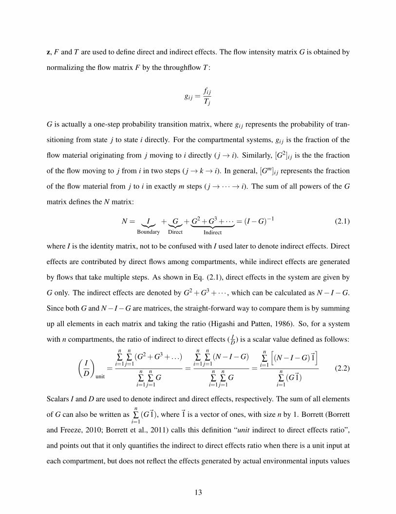
z, F and T are used to define direct and indirect effects. The flow intensity matrix G is obtained by

normalizing the flow matrix F by the throughflow T :

gi j =fi j

Tj

G is actually a one-step probability transition matrix, where gi j represents the probability of tran-

sitioning from state j to state i directly. For the compartmental systems, gi j is the fraction of the

flow material originating from j moving to i directly ( j→ i). Similarly, [G2]i j is the the fraction

of the flow moving to j from i in two steps ( j→ k→ i). In general, [Gm]i j represents the fraction

of the flow material from j to i in exactly m steps ( j→ ··· → i). The sum of all powers of the G

matrix defines the N matrix:

N = I︸︷︷︸Boundary

+ G︸︷︷︸Direct

+ G2 +G3 + · · ·︸ ︷︷ ︸Indirect

= (I−G)−1 (2.1)

where I is the identity matrix, not to be confused with I used later to denote indirect effects. Direct

effects are contributed by direct flows among compartments, while indirect effects are generated

by flows that take multiple steps. As shown in Eq. (2.1), direct effects in the system are given by

G only. The indirect effects are denoted by G2 +G3 + · · · , which can be calculated as N− I−G.

Since both G and N− I−G are matrices, the straight-forward way to compare them is by summing

up all elements in each matrix and taking the ratio (Higashi and Patten, 1986). So, for a system

with n compartments, the ratio of indirect to direct effects ( ID ) is a scalar value defined as follows:

(ID

)unit

=

n∑

i=1

n∑j=1

(G2 +G3 + . . .)

n∑

i=1

n∑j=1

G=

n∑

i=1

n∑j=1

(N− I−G)

n∑

i=1

n∑j=1

G=

n∑

i=1

[(N− I−G)~1

]n∑

i=1(G~1)

(2.2)

Scalars I and D are used to denote indirect and direct effects, respectively. The sum of all elements

of G can also be written asn∑

i=1(G~1), where~1 is a vector of ones, with size n by 1. Borrett (Borrett

and Freeze, 2010; Borrett et al., 2011) calls this definition “unit indirect to direct effects ratio”,

and points out that it only quantifies the indirect to direct effects ratio when there is a unit input at

each compartment, but does not reflect the effects generated by actual environmental inputs values

13

(z). He defines “realized indirect to direct effects ratio”, where the matrices are weighted and

dimensionalized with environmental inputs (z) before computing the summation:

(ID

)realized

=

n∑

i=1

[(G2 +G3 + . . .)z

]n∑

i=1(Gz)

=

n∑

i=1[(N− I−G)z]

n∑

i=1(Gz)

(2.3)

2.3 Pathway-based definition for ID ratio

2.3.1 From flows to pathways

As shown in the previous section, the two conventional definitions for ID are computed using matrix

algebra. Both definitions are similar in that the denominator quantifies one-step relations (direct

effects D), and the numerator computes multiple-step relations (indirect effects I). The difference

lies in how they derive scalar quantities to represent direct and indirect effects. The original defi-

nition simply adds the matrix entries, whereas the realized definition uses inputs (z) as weighting

terms. This brings out the question of an optimal weighting term to quantify indirect to direct ef-

fects ratio. How can we figure out the optimal mathematical formulations for I and D that quantify

the indirect and direct flow interactions? This is not an easy question, simply because the algebraic

formulations are rather unintuitive. It is difficult to grasp what Eqs. (2.2) and (2.3) actually rep-

resent. However, we have no other choice, given that the ecological models are represented with

flow rates (F), inputs (z) and outputs (y).

To pursue a solution, we temporarily discard the conventional representation of ecological models,

and try to find a more natural way to study this measure. The system is generally considered as

continuous flows of energy or matter. From another angle, these continuous flows can be regarded

as numerous discrete energy-matter quanta passing through the system. We call such small unit of

discrete flow material particle. Particle pathways within a system are similar to food chains. In

each pathway, a direct flow from one compartment to another constitutes a direct effect. If the flow

14

* 1 2 3 1 2 *

2 steps

4 steps

3 steps

Figure 2.2: Counting direct and indirect relations in a pathway of a single quantum from the three-compartment model shown in Figure 2.1. The numbers 1, 2 and 3 correspond to the compartmentsProducers, Consumers, and Nutrient Pool. Arrows at both ends are environmental input and output.

material from one compartment reaches another through other compartments in multiple steps, this

constitutes an indirect effect. Both direct and indirect effects depend on the relationships within

the system. Therefore, boundary environmental inputs and outputs are not involved in this regard.

Figure 2.2 is the pathway of a single particle (energy-matter quantum) in the Figure 2.1 system.

This particle goes through compartments 1, 2, 3 and then cycles back to 1, and leaves the system at

2. The black arrows represent the direct relations: 1 on 2, 2 on 3, 3 on 1, and 1 on 2. The number

of direct relations is four. Colored arrows show multiple-step relations. There exist three two-step

relations (1 on 3, 2 on 1, and 3 on 2), two three-step relations (1 on 1 and 2 on 2) and one four-step

relation (1 on 2), all of which are counted as indirect relations. Therefore, the number of indirect

effects is six.

Figure 2.2 only shows one possible pathway a particle can travel. There are infinitely many differ-

ent pathways even for this simple model. So, to accurately count indirect and direct effects for an

entire ecosystem, we need to find out all possible pathways, and how frequently each pathway is

utilized. The problem is how to derive this infinite set of chains, which are equivalent to the whole

system.

Network Particle Tracking (NPT) (Kazanci et al., 2009; Tollner et al., 2009) is an individual

based simulation method, where discrete quanta (particles) of material or energy are numbered

and tracked in time as they are sequentially transferred through the model compartments. NPT

15

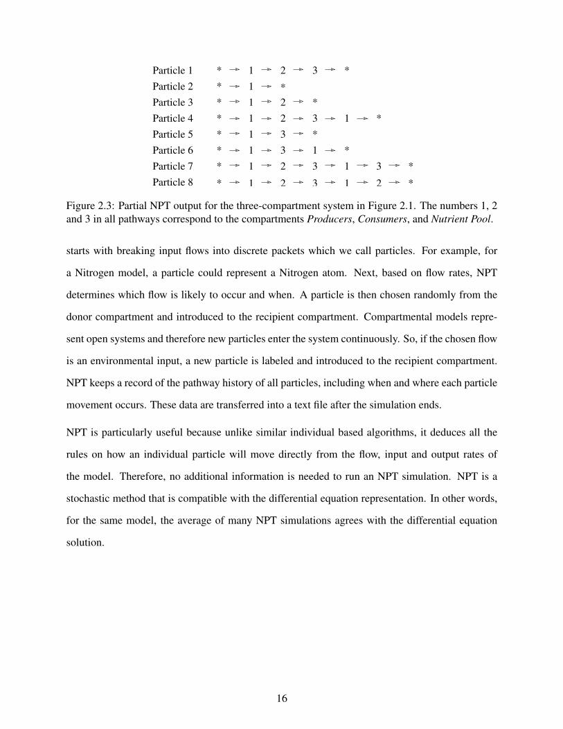
1 2* 3 *

* 1

* 1 2 *

* 1 2 3 1

* 1 3 *

*

*

* 1 3 1 *

* 1 2 3 1 3 *

* 1 2 3 1 2 *

Particle 1

Particle 2

Particle 3

Particle 4

Particle 5

Particle 6

Particle 7

Particle 8

Figure 2.3: Partial NPT output for the three-compartment system in Figure 2.1. The numbers 1, 2and 3 in all pathways correspond to the compartments Producers, Consumers, and Nutrient Pool.

starts with breaking input flows into discrete packets which we call particles. For example, for

a Nitrogen model, a particle could represent a Nitrogen atom. Next, based on flow rates, NPT

determines which flow is likely to occur and when. A particle is then chosen randomly from the

donor compartment and introduced to the recipient compartment. Compartmental models repre-

sent open systems and therefore new particles enter the system continuously. So, if the chosen flow

is an environmental input, a new particle is labeled and introduced to the recipient compartment.

NPT keeps a record of the pathway history of all particles, including when and where each particle

movement occurs. These data are transferred into a text file after the simulation ends.

NPT is particularly useful because unlike similar individual based algorithms, it deduces all the

rules on how an individual particle will move directly from the flow, input and output rates of

the model. Therefore, no additional information is needed to run an NPT simulation. NPT is a

stochastic method that is compatible with the differential equation representation. In other words,

for the same model, the average of many NPT simulations agrees with the differential equation

solution.

16

Table 2.1: Computation of direct and indirect effects based on the pathways in Figure 2.3.Particle #s 1 2 3 4 5 6 7 8 Sum

Direct relations 2 0 1 3 1 2 4 4 17Indirect relations 1 0 0 3 0 1 6 6 17

2.3.2 A pathway-based formulation

Figure 2.3 shows a partial NPT simulation output for the three-compartment system in Figure 2.1.

Pathways visited by eight particles are listed. We randomly choose these eight pathways to show

the computation of indirect (I) and direct (D) effects. The same method can be applied to any other

set of pathways. In Table 2.1, we compute the direct and indirect relations for each pathway. Then

ID is computed as the sum of all indirect relations divided by the sum of all direct relations. So the

indirect to direct effects ratio isID

=1717

= 1

The same information presented in Table 2.1 can also be represented in the form of two matrices

(direct flow and indirect flow), as shown in Table 2.2. Each entry represents the number of direct

and indirect relations among compartment pairs. Column compartments are donors, and row com-

partments are recipients. For example, 6 in column “Comp 1” and row “Comp 2” represents the

six direct flows from compartment 1 to compartment 2. The sum of all entries in each matrix is

both 17 and therefore the ID is one.

Information in Table 2.1 and Table 2.2 is equivalent in computing the overall I/D ratio. However,

compared to Table 2.1, Table 2.2 has an advantage of comparing direct and indirect effects between

any two compartments. For example, from this partial output, the number of direct and indirect

flow from “Comp 1” to “Comp 3” are 3 and 5. For these two compartments, indirect effects

17

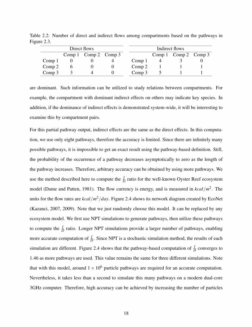
Table 2.2: Number of direct and indirect flows among compartments based on the pathways inFigure 2.3.

Direct flowsComp 1 Comp 2 Comp 3

Comp 1 0 0 4Comp 2 6 0 0Comp 3 3 4 0

Indirect flowsComp 1 Comp 2 Comp 3

Comp 1 4 3 0Comp 2 1 1 1Comp 3 5 1 1

are dominant. Such information can be utilized to study relations between compartments. For

example, the compartment with dominant indirect effects on others may indicate key species. In

addition, if the dominance of indirect effects is demonstrated system-wide, it will be interesting to

examine this by compartment pairs.

For this partial pathway output, indirect effects are the same as the direct effects. In this computa-

tion, we use only eight pathways, therefore the accuracy is limited. Since there are infinitely many

possible pathways, it is impossible to get an exact result using the pathway-based definition. Still,

the probability of the occurrence of a pathway decreases asymptotically to zero as the length of

the pathway increases. Therefore, arbitrary accuracy can be obtained by using more pathways. We

use the method described here to compute the ID ratio for the well-known Oyster Reef ecosystem

model (Dame and Patten, 1981). The flow currency is energy, and is measured in kcal/m2. The

units for the flow rates are kcal/m2/day. Figure 2.4 shows its network diagram created by EcoNet

(Kazanci, 2007, 2009). Note that we just randomly choose this model. It can be replaced by any

ecosystem model. We first use NPT simulations to generate pathways, then utilize these pathways

to compute the ID ratio. Longer NPT simulations provide a larger number of pathways, enabling

more accurate computation of ID . Since NPT is a stochastic simulation method, the results of each

simulation are different. Figure 2.4 shows that the pathway-based computation of ID converges to

1.46 as more pathways are used. This value remains the same for three different simulations. Note

that with this model, around 1× 106 particle pathways are required for an accurate computation.

Nevertheless, it takes less than a second to simulate this many pathways on a modern dual-core

3GHz computer. Therefore, high accuracy can be achieved by increasing the number of particles

18

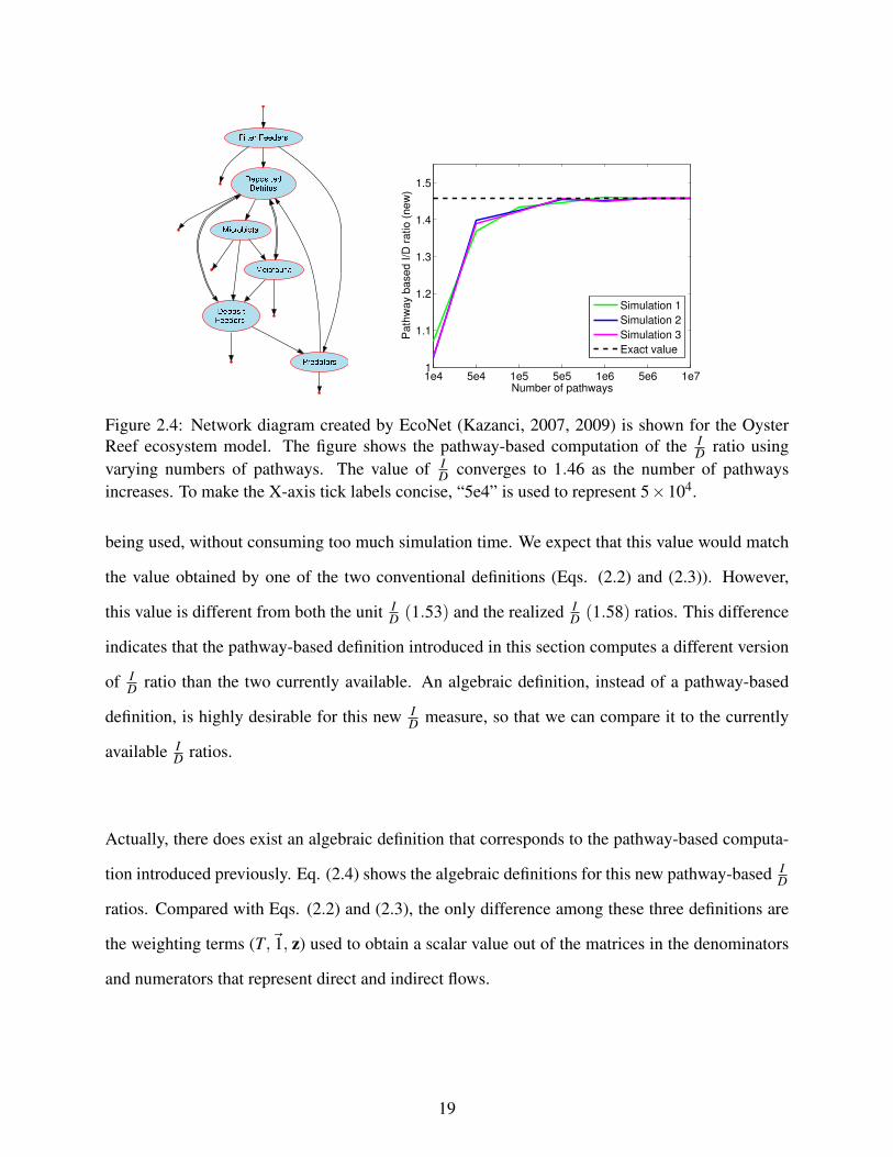
1e4 5e4 1e5 5e5 1e6 5e6 1e71

1.1

1.2

1.3

1.4

1.5

Number of pathways

Path

way b

ased I/D

ratio (

new

)

Simulation 1

Simulation 2

Simulation 3

Exact value

Figure 2.4: Network diagram created by EcoNet (Kazanci, 2007, 2009) is shown for the OysterReef ecosystem model. The figure shows the pathway-based computation of the I

D ratio usingvarying numbers of pathways. The value of I

D converges to 1.46 as the number of pathwaysincreases. To make the X-axis tick labels concise, “5e4” is used to represent 5×104.

being used, without consuming too much simulation time. We expect that this value would match

the value obtained by one of the two conventional definitions (Eqs. (2.2) and (2.3)). However,

this value is different from both the unit ID (1.53) and the realized I

D (1.58) ratios. This difference

indicates that the pathway-based definition introduced in this section computes a different version

of ID ratio than the two currently available. An algebraic definition, instead of a pathway-based

definition, is highly desirable for this new ID measure, so that we can compare it to the currently

available ID ratios.

Actually, there does exist an algebraic definition that corresponds to the pathway-based computa-

tion introduced previously. Eq. (2.4) shows the algebraic definitions for this new pathway-based ID

ratios. Compared with Eqs. (2.2) and (2.3), the only difference among these three definitions are

the weighting terms (T,~1, z) used to obtain a scalar value out of the matrices in the denominators

and numerators that represent direct and indirect flows.

19

(ID

)new

=

n∑

i=1

[(G2 +G3 + · · ·)T

]n∑

i=1(GT )

(2.4)

The pathway-based definition we formulated uses throughflows (T ) as the weighting term. The

direct effects for the new ID ratio is computed as:

n

∑i=1

(GT ) =n

∑i=1

f11T1

f12T2· · · f1n

Tn

f21T1

f22T2· · · f2n

Tn

...... . . . ...

fn1T1

fn2T2· · · fnn

Tn

T1

T2

...

Tn

=

n

∑i=1

n

∑j=1

fi j

The product of G and T is exactly the sum of all direct flows (per unit time) in the system. Think-

ing about G as a probability matrix, it becomes clear that G2 represents the probability that two

consecutive flows occur. Then the product [G2]i jTj represents the amount of indirect flow from j

to i over two steps. Considering all powers of G, the product of ([G2]i j +[G3]i j + · · · ) and Tj equals

the total indirect flows from j to i per unit time. So, the indirect effects in the entire system are:

n

∑i=1

n

∑j=1

[([G2]i j +[G3]i j + · · ·)Tj

]=

n

∑i=1

[(G2 +G3 + · · ·)T

]We showed that this new formulation captures the ratio of direct to indirect flows, and therefore

reflects the intended meaning of ID ratio more accurately. Then, the similar yet different two

definitions using~1 and Z as their weighting term compute something different. Unfortunately, the

complexity of the algebraic formulations in Eq. (2.4) provide little insight as to how these three

ID measures differ in reality. On the other hand, pathway-based definitions are simple, intuitive,

insightful and informative. In the next section, we construct pathway-based definitions for the two

conventional ID measures, which clearly reveal what actually is being computed from a particle or

quantum point of view.

20

2.4 Pathway-based formulations for conventional ID measures

2.4.1 Pathway-based formulation for the conventional (unit) ID ratio

The new ID ratio (Eq. (2.4)) uses throughflow values (T ) as weighting terms to compute the direct

and indirect effects. However, the unit definition (Eq. (2.2)) uses ones as a weighting term, and

directly adds up all the entries in the G matrix. Recall that each entry of [Gn]i j represents the

fraction of flow from j to i over n steps. Therefore, to compute the unit ID ratio using pathways,

we can use the same counting algorithm we used in the previous section. However, we will need

to reverse the throughflow weighting term by normalizing all the counts by the throughflow. In

order to construct a pure pathway-based definition, we need to compute throughflows using the

pathways as well.

Using the same partial pathway output in Figure 2.3, three compartments appear 12, 6, and 7

times, respectively. This means 12 times particles go through compartment 1, 6 times through

compartment 2, and 7 times through compartment 3. So in this data set, the sum of throughflow at

three compartments are 12, 6, and 7, respectively. To get the unit definition, we need to normalize

the counts of direct and indirect relations in Table 2.2 by throughflow T . Each entry in Table 2.2

is divided by throughflow at the column compartment, which is the donor in the relation. For

example, the direct flow from compartment 1 to compartment 2 is 6 particles. The throughflow at

compartment 1 is 12 particles. So 6/12 = 50% of T1 goes to compartment 2.

The normalized direct and indirect flows are the direct and indirect flow generated by per unit

throughflow at the donor compartment. This corresponds to the meaning of matrix G and G2 +

G3 + · · · . Then direct effects D is the sum of all entries in normalized direct flows in the Table 2.3,

and indirect effects I is the summation of all entries in the normalized indirect flows in the Table

2.3. The indirect effect ratio is ID is the ratio of these two quantities.

21

Table 2.3: Normalization of direct and indirect flow counts by throughflow, where throughflowT = [12, 6, 7].

Normalized direct flowsComp 1 Comp 2 Comp 3

Comp 1 0 0 4/7Comp 2 6/12 0 0Comp 3 3/12 4/6 0

Normalized indirect flowsComp 1 Comp 2 Comp 3

Comp 1 4/12 3/6 0Comp 2 1/12 1/6 1/7Comp 3 5/12 1/6 1/7

While it seems natural to add up all the entries in the G matrix to compute the direct effects, we

learn from the pathway-based formulation that the throughflow weighting term is indeed needed

to compare the actual direct and indirect flows. Therefore this new formulation presented in this

paper is more correct in assessing flows (F), rather than flow intensities (G).

2.4.2 Pathway-based formulation for the input-driven (realized) ID ratio

The realized definition in Eq. (2.3) is weighted by environmental input z. In this definition, if

one entry zi = 0, all entries g ji ( j = 1, · · · , n) are not counted in computing direct effects, and all

entries [G2 +G3 + · · · ] ji ( j = 1, · · · , n) are also eliminated from indirect effects. This definition

only counts the relations starting with environmental input. All the other relations are effectively

zeroed. As shown in Figure 2.5, the environmental input happens at 1. There is only one direct

relation: 1 on 2. Three indirect relations are 1 on 3, 1 on 1, and 1 on 2 with lengths 2, 3, and 4,

respectively. All the other relations are not considered in this situation. Compared with Figure 2.2,

three indirect relations (2 on 1, 2 on 2, and 3 on 2) and three direct relations (2 on 3, 3 on 1, and 1

and 2) are nullified by zero inputs.

Using the partial output in Figure 2.3, the accounting of direct and indirect relations is shown in

Table 2.4. This is very different from that in Table 2.1. Both the numbers of direct and indirect

relations decrease. Then( I

D

)realized = 10

7 is different from( I

D

)new = 17

17 . Based on the insight

22

* 1 2 3 1 2 *

4 steps

2 steps

3 steps

Figure 2.5: Counting direct and indirect relations in one pathway for the three-compartment modelin Figure 2.1. The numbers 1, 2 and 3 correspond to compartments Producers, Consumers, andNutrient Pool.

Table 2.4: Computation of direct and indirect relations starting at compartment 1 only.Particle #s 1 2 3 4 5 6 7 8 Sum

Direct relations 1 0 1 1 1 1 1 1 7Indirect relations 1 0 0 2 0 1 3 3 10

gained from this pathway-based analysis, we will refer to the realized ID ratio as input-driven I

D

ratio.

2.4.3 Accuracy and convergence of pathway-based formulations for two con-

ventional ID measures

To check whether our explanations are correct, we calculate two conventional definitions with NPT

pathways for the twenty models in Table 2.5. We observe that pathway-based definitions do match

with their algebraic versions (Eq. (2.4)). For demonstration purposes, we use the Oyster Reef

ecosystem model (Dame and Patten, 1981) to show the convergence and accuracy properties of the

pathway-based definitions for the two conventional measures. Using the regular method, unit ID is

1.53 and input-driven ID is 1.58. As we increase the number of pathways used for computations,

both the unit ID and input-driven I

D converge to the results from conventional methods, shown in

Figure 2.6.

23

1e4 5e4 1e5 5e5 1e6 5e6 1e71

1.1

1.2

1.3

1.4

1.5

1.6

Number of pathways

Unit I/D

ratio

(a)

Simulation 1

Simulation 2

Simulation 3

Exact value

1e4 5e4 1e5 5e5 1e6 5e6 1e71

1.1

1.2

1.3

1.4

1.5

1.6

Number of pathways

Input

driven

I/D

ra

tio

(b)

Simulation 1

Simulation 2

Simulation 3

Exact value

Figure 2.6: Accuracy plots for two conventional definitions. As the number of pathways increases,unit I

D converges to 1.53 and input-driven (realized) ID converges to 1.58.

This verifies that our explanations for these two definitions using pathways are indeed correct.

The conventional definitions have a clear meaning from a pathway point of view. Borrett et al.

(2011) states “the unit method assumes that each node receives a single unit of input”. Pathway-

based analysis indicates that perhaps a more specific and accurate meaning for “unit” here is “unit

throughflow”, including both environmental inputs and inter-compartment inputs (inflows).

2.5 Normalization and comparison of the three ID formulations

In this paper, we cover three different ID ratio formulations. One common issue to all three for-

mulations is the range of these indices. ID ratio can take any value from zero to infinity. Larger I

D

ratio means stronger indirect effects. Zero means no indirect effects. Direct effects are dominant

if ID is less than one. Otherwise, if I

D is larger than one, indirect effects are dominant. Higashi

and Patten (1989) and Salas and Borrett (2011) show that indirect effects in ecological networks

are significantly dominant. However, arbitrarily large ID ratios make comparison among models

difficult. Therefore we suggest a rescaling of the current measure, representing the fraction of the

24

indirect effects compared to the total of direct and indirect effects:

IEI =I

I +D=

( ID

)1+( I

D

) (2.5)

We call this new ratio, indirect effects index (IEI). Similar to Finn’s cycling index, the new mea-

sure ranges between 0 and 1. Actually, similar to ID ratio, the initial definition of cycling index

(Finn, 1976) ranged from zero to infinity. This original definition was later revised by Finn (Finn,

1980) in the exact way that we propose to rescale the ID ratio. For example, the new I

D ratios for

the Aggregated Baltic Ecosystem and Temperate Forest ecosystem model (Table 2.5) are 1.772

and 27.133, respectively. For the same models, indirect effects indices ( II+D ) are 0.639 and 0.965.

Comparison between models becomes easier and more accessible using IEI since it reflects per-

centages. To show how the three formulations of ID ratios and the associated indirect effect indices

II+D compare, we compute them for twenty ecosystem models (Table 2.5), all at steady state.

Figure 2.7 shows all three IEIs and FCI together for twenty models. We observe that for models

with high FCI, the values of the three formulations are not significantly different. We believe this

is due to the homogenization property (Fath and Patten, 1999a) of well connected networks with

high cycling indices, where the differences between individual compartmental throughflows are

less pronounced.

The difference is larger for models with low cycling indices, such as the North Sea and the Silver

Springs models shown in Table 2.5. Furthermore, we observe that the relation between the con-

ventional and the new (revised) indirect effect index is not uniform across models. In other words,

for a given model, it is not at all certain which index will be higher than the other. For exam-

ple, let’s consider the Generic Freshwater Stream Ecosystem and Cypress Wet Season Ecosystem

models (the third and fourth models in Figure (2.7)). Using the unit definition IEI(I), Cypress Wet

Season Ecosystem has almost twice the II+D value of the Generic Freshwater Stream Ecosystem.

However, applying our new IEI(T), Generic Freshwater Stream Ecosystem has a slightly higher

25

Tabl

e2.

5:T

heth

ree

form

ulat

ions

for

the

I Dra

tio,t

heas

soci

ated

indi

rect

effe

ctin

dice

s(I

EI)

,and

the

Finn

Cyc

ling

Inde

x(F

CI)

show

nfo

rtw

enty

ecos

yste

mm

odel

s.

Mod

elFl

owcu

rren

cy

I DI

I+D

FCI

Uni

tIn

putd

riven

New

Uni

tIn

putd

riven

New

Nor

thSe

a(S

teel

e,19

74)

Ene

rgy

0.37

10.

754

0.61

60.

271

0.43

00.

382

0Si

lver

Spri

ngs

(Odu

m,1

957)

Ene

rgy

0.08

40.

204

0.17

80.

077

0.17

00.

151

0G

ener

icFr

eshw

ater

Stre

amE

cosy

stem

Web

ster

etal

.(19

75a)

Min

eral

0.58

71.

357

0.78

20.

370

0.57

60.

439

0.00

1C

ypre

ssW

etSe

ason

(Ula

now

icz,

1997

)C

arbo

n1.

709

0.62

30.

710

0.63

10.

384

0.41

50.

044

Eve

glad

esG

ram

inoi

dD

rySe

ason

(Ula

now

icz,

1999

)C

arbo

n1.

001

1.40

80.

898

0.50

00.

585

0.47

30.

046

Nor

ther

nB

engu

ela

Upw

ellin

g(H

eym

ans

and

Bai

rd,2

000)

Car

bon

0.40

31.

043

0.87

80.

291

0.51

40.

468

0.04

7C

ryst

alC

reek

(Ula

now

icz,

1986

b)C

arbo

n0.

617

0.67

20.

643

0.38

20.

402

0.39

10.

066

Flor

ida

Bay

Trop

hic

Exc

hang

eM

atri

x(U

lano

wic

z,19

98)

Car

bon

1.45

61.

289

1.19

70.

593

0.56

30.

545

0.08

4C

ryst

alR

iver

Cre

ek(U

lano

wic

z,19

86b)

Car

bon

0.68

90.

709

0.75

50.

408

0.41

50.

430

0.09

0C

one

Spri

ng(T

illy,

1968

)E

nerg

y0.

913

1.02

30.

859

0.47

70.

506

0.46

20.

092

Neu

seE

stua

ryN

etw

ork

Mod

elC

arbo

n2.

443

1.48

21.

661

0.71

00.

597

0.62

40.

116

Agg

rega

ted

Bal

ticE

cosy

stem

(Wul

ffan

dU

lano

wic

z,19

89)

Car

bon

1.53

01.

902

1.77

20.

605

0.65

50.

639

0.12

9So

mm

eE

stua

ry(R

ybar

czyk

and

Now

akow

ski,

2003

)C

arbo

n0.

674

0.73

60.

853

0.40

30.

424

0.46

00.

139

Flor

ida

Bay

Wet

Seas

on(U

lano

wic

z,19

98)

Car

bon

1.90

41.

733

1.63

20.

656

0.63

40.

620

0.14

4Y

than

Est

uary

(Bai

rdan

dM

ilne,

1981

)C

arbo

n2.

143

1.88

41.

950

0.68

20.

653

0.66

10.

225

Lak

eW

ingr

a(R

iche

yet

al.,

1978

)C

arbo

n1.

903

1.79

91.

927

0.65

60.

643

0.65

90.

396

Trop

ical

Rai

nFo

rest

(Edm

iste

n,19

70)

Nitr

ogen

6.18

46.

140

6.07

30.

861

0.85

90.

859

0.47

9Pu

erto

Ric

anR

ain

Fore

st(J

orda

net

al.,

1972

)C

alci

um6.

394

7.74

16.

610

0.86

50.

886

0.86

90.

569

Gen

eric

Tund

raE

cosy

stem

(Web

ster

etal

.,19

75a)

Min

eral

23.6

0125

.553

23.9

160.

959

0.96

20.

959

0.81

6Te

mpe

rate

Fore

st(W

ebst

eret

al.,

1975

a)M

iner

al26

.881

28.5

3927

.133

0.96

40.

966

0.96

50.

833

26

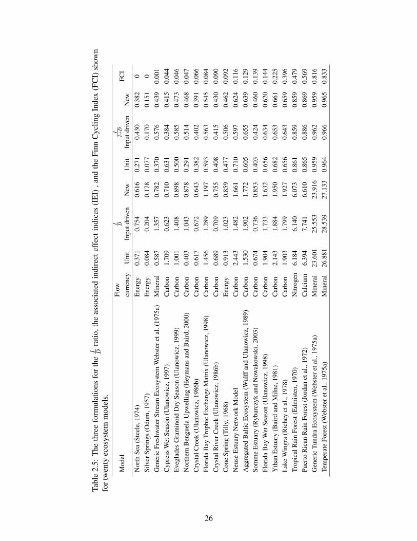
0 5 10 15 200

0.2

0.4

0.6

0.8

1

Models

Va

lue

s f

or

FC

I a

nd

IE

I

IEI (I)

IEI (Z)

IEI (T)

FCI

Figure 2.7: Comparison of the three indirect effects indices (IEI, Eqs. 2.4 and 2.5) and the cyclingindex (FCI) for the twenty ecosystem models presented in Table 2.5.

value. Therefore, if a study comparing these two ecosystems used the old index IEI(I), the conclu-

sion that one of the models has almost twice the indirect effects of the other one would be wrong.

One of the main uses of ENA measures is to compare ecosystems (Ray, 2008), and this work

has significant implications for past and future studies using indirect effects ratio as a measure

for comparison purposes. EcoNet© (http://eco.engr.uga.edu) computes the new revised IEI

definition presented here as well as the older definitions.

Pathway-based analysis of three different ID ratios gives better understanding of this measure. The

unit definition quantifies indirect and direct flows generated by per unit throughflow but not the

actual flows. So the unit ID could be called as indirect and direct flow intensities. The input-based

definition quantifies indirect and direct flows generated by dimensioned environmental inputs. This

omits any indirect and direct flows not initiated by environmental input but exists among compart-

ments. The new throughflow-weighted definition is the most natural and intuitive one, which is

also the only one indeed computing the actual indirect and direct flow ratio. Hence, our study re-

27

vises earlier formulations while retaining the original conception of ID ratios as a way of comparing

direct and indirect effects.

2.6 Conclusion

Since its inception the conceptualization of indirect effects has been based on pathways, but its

formulation required rather complicated algebraic input-output formulations. Thanks to recent ad-

vances in computational resources, and efficient numerical algorithms (NPT), we are now able to

compute direct and indirect effects literally as conceptualized. The methodology provides compu-

tational accuracy and conceptual clarity.

The same approach has been successfully applied to Finn’s cycling index (Kazanci et al., 2009),

throughflow analysis (Matamba et al., 2009) and storage analysis (Kazanci and Ma, 2012). In all

three cases, the results of the pathway-based definition matched the algebraic formulation, verify-

ing the accuracy of both methods. Pathway-based definitions are more intuitive, straightforward

and simple. Therefore, the agreement of both results also shows that the rather complicated alge-

braic formulations do indeed reflect their intended meaning. However, in the case of ID ratio, there

was a discrepancy between both methodologies. Our investigation has led to a revised algebraic

formulation (Eq. (2.4)) which, by present analysis, seems more accurately to reflect accurately

reflects the intended meaning of the ID ratio.

To investigate the issue in detail, we constructed pathway-based definitions for the two current ID

ratio formulations. These inform us how the algebraic formulations represent ID from a pathway

perspective, clarifying conceptually exactly what is being computed. From the analysis of twenty

ecosystem models, the three formulations are numerically close, especially when a significant

amount of cycling exists. The mathematical reason for this similarity might be due to the fact

that all three definitions are based on powers of the G matrix, but with different weighting terms.

However, three definitions are vastly different for low cycling models. Our new definition could

possibly reverse some previous conclusions based on original ones.

28

This study is complete in the sense that all three pathway-based NPT formulations have corre-

sponding algebraic NEA counterparts. However, further studies can focus on indirect effects be-

tween compartments. As we referred to in Section 3.2, the ID ratio between any two compartments

is available without further computation. It might have many interesting applications, such as

identifying the key species in the ecosystem. If one species has very high indirect effects on other

species, this indicates it is possibly the key species in the system.

While our focus here has been indirect effects, this work also demonstrates just how useful pathway-

based methodologies can be. In this current and our past studies, we noticed that the pathway-based

formulations are often easier, simpler, and more intuitive than their algebraic counterparts. It has

been our experience that the pathway-based methodology provides a more flexible and potentially

useful framework for ecological network analysis compared to using aggregated values (flow ma-

trix, environmental inputs and outputs). The pathway-based methodology has proved to be a pow-

erful tool, not replacing, but complementing the algebraic framework developed over the years.

The pathway-based methodology is made possible largely by the NPT algorithm. Generating the

pathway data out of the flow, input and output values is a necessity, which can be a tedious task.

However, less computation-intensive alternatives to NPT algorithm exists, and our future work will

focus on such methods. A significant advantage of the NPT algorithm is its ability to extend the

applicability of steady-state network measures to dynamic and non-linear models. Many essential

and interesting issues involve change, such as environmental impacts, climate change and regime

shifts. It is possible to utilize network metrics like the cycling index, throughflow analysis, storage

analysis, and now the indirect effects index to tackle such issues.

29

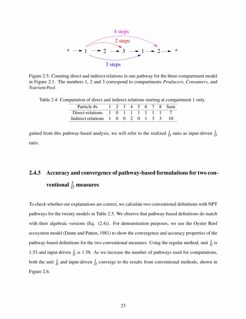
Chapter 3

How much of the storage in the ecosystem isdue to cycling?1

1Ma, Q. and Kazanci, C. Accepted by Journal of Theoretical Biology. Reprinted here with permission of publisher.

30

Abstract

Cycling is the process of reutilization of matter or energy in the ecosystem. As it is not directly

measurable, the strength of cycling is calculated based on mathematical models of the ecosystem.

For a storage-flow type ecosystem model, throughflow is the total amount of material flowing

through all system compartments per unit of time, while storage represents the total standing stock

in the system. Finn’s cycling index (FCI) is widely used to measure the cycled throughflow, the

proportion of throughflow generated by cycling. Thus, although originally named after its author

J. T. Finn, FCI can also be called a “flow-based” cycling index. In addition to flow, storage plays

an important role in generating network properties, and therefore should be taken into account in

measuring cycling. In this paper, we investigate how much of the total standing stock of matter or

energy in the ecosystem is due to cycling, and formulate a storage-based cycling index (SCI), by

utilizing an individual-based method to simulate the system. SCI utilizes flow values used for FCI

and takes into account residence time as well. Therefore, SCI is a preferable index for quantifying

cycling in ecosystems.

3.1 Introduction

Cycling of nutrients in ecosystems (Odum, 1971), such as carbon, phosphorus and nitrogen cy-

cles, has been widely investigated in the last several decades. Despite some disagreement (Odum,

1971), energy also cycles in the ecosystem (Patten, 1985a, 1986), but probably not in as significant

amounts as matter. The cycling of energy is mainly accomplished by transfer and transforma-

tion of energy in dead organic matter (detritus), and back to the system through detritus feeders

(Fath and Halnes, 2007). Energy cycling can also be realized by cannibalism, which occurs in a

variety of taxa, but is especially prevalent in fishes with parental care (FitzGerald, 1992). Many

studies on cycling in ecosystems (Fenchel et al., 1979; DeAngelis, 1980) have been devoted to

31

the empirical description of specific cycling processes, such as the detailed pathways of carbon,

phosphorus and nitrogen cycles. In this paper, we focus on quantifying this important measure for

a general ecosystem model of any conservative flow currency, such as biomass, nutrients, energy,

or a specific element such as carbon, nitrogen or phosphorus.

According to Odum (1969), cycling is an indicator of maturity of an ecosystem. It reveals the

ecosystem’s ability to retain matter or energy, and to endure in the face of resource scarcity. Several

studies (DeAngelis, 1980; DeAngelis et al., 1989; Loreau, 1994) indicate that increasing material

cycling tends to increase the probability that the system will be locally stable. Scotti (2008) points

out that increasing the amount of recycled matter tends to increase transfer efficiency and minimize

the ecosystem’s dependence on external supports. Depending on the flow currency, the effect of

cycling may be interpreted differently. For nitrogen and phosphorus, it means efficient utilization

of nutrients (Vitousek, 1982). For carbon, high cycling may indicate a stressed system (Wulff

and Ulanowicz, 1989). High cycling in a stressed system is mostly through shorter cycles, while

the similar cycling values tend to be realized through longer paths in mature systems (Baird and

Ulanowicz, 1993; Christian et al., 2005; Scotti, 2008). Therefore, quantifying cycling in ecosys-

tems is of great importance to evaluate how well the ecosystem functions. However, measuring

the strength of cycling is not trivial. One reason is that, unlike many other ecological indicators,

the strength of cycling cannot be measured directly, as its occurrence depends on indirect flows,

which are mediated or transmitted through other compartments. For example, even the shortest

cycle, such as A→ B→ A, requires indirect flows that are transmitted by B.

Most efforts on developing a cycling index are based on mathematical models that describe the

flow of energy or matter among a variety of species. While cycling can simply be defined as the re-

utilization of flow material, there are multiple ways to quantify the strength of cycling (Finn, 1976;

Patten and Higashi, 1984; Allesina and Ulanowicz, 2004). For example, Finn’s cycling index (FCI)

(Finn, 1976, 1978) calculates the proportion of total system throughflow of energy or matter that

is generated by cycling. Allesina and Ulanowicz (2004) proposes a comprehensive cycling index

(CCI) that takes into account cycling paths, including simple cycles, compound paths and com-

32

pound cycles. Simple paths are defined as paths with no repeated compartments; simple cycles are

simple paths in which the starting and the ending compartments coincide; compound paths are the

paths with repeated compartments; and compound cycles are repeated cycles. A different approach

by Ulanowicz (1983) quantifies the amount of cycling by subtracting the structure of cycling from

the entire network. All simple cycles are subtracted from the network until the remaining network

becomes acyclic.

Among various cycling indices, the most widely accepted and used one is Finn’s cycling index

(FCI) (Finn, 1976, 1978). This index is part of ecological network analysis (ENA) (Patten, 1978;

Fath and Patten, 1999b; Ulanowicz, 2004), a system-oriented methodology to analyze within-

system interactions (Fath and Borrett, 2006). ENA works with the representations of ecosystems as

compartmental models, where compartments and connections represent various species and flows

of matter or energy, respectively. ENA defines various quantitative indicators, including FCI,

to describe different aspects of the ecosystem. Most of these indicators provide the description

of non-observable relations within the system. For example, indirect effect index (IEI) repre-

sents the proportion of indirect effects over the total effects (Higashi and Patten, 1989; Ma and

Kazanci, 2012a); throughflow analysis (N matrix) (Matamba et al., 2009) and storage analysis (S

matrix) (Fath and Patten, 1999b) respectively calculate how the environmental inputs contribute

to throughflow and storage of each compartment in the system. Most of these measures involve

somewhat unintuitive matrix computations, and are only applicable to steady-state systems, where

the flow and storage values stay constant over time. In contrast to the algebraic method used in

ENA, an individual-based simulation method, network particle tracking (NPT), has been used to

study most ENA indicators and offer simpler and more intuitive interpretations of these proper-

ties (Kazanci et al., 2009; Matamba et al., 2009; Ma and Kazanci, 2012a,b). As NPT is based on

Gillespie’s stochastic algorithm (Gillespie, 1977) for simulating chemical reactions, the mean of

different NPT simulations for the same model agree with the differential equation model. Simu-

lating tracer experiments, NPT discretizes storages of energy or mass into particles (e.g., single

atoms and energy quanta) and provides a list of pathways that particles pass through in the ecosys-

33

tem. Furthermore, utilizing NPT, Kazanci (2011) extends some ENA measures to dynamic models,

significantly increasing their applicability.

FCI is defined using an algebraic formula (Eq. (3.4)). While this algebraic definition of cycling

is computationally efficient for steady-state models, it is rather hard to build an intuitive link be-

tween the concept of cycling and the formula itself. For example, Allesina and Ulanowicz (2004)

states that “FCI is a biased counting of cycling, because it does not include all flows engaged in

recycling”. While FCI does indeed compute the fraction of cycled throughflow through all in-

direct flows, this fact is not immediately recognizable from its algebraic formula. Using NPT,

Kazanci et al. (2009) confirms that FCI does actually compute the fraction of all particles’ revisits

to compartments (system throughflow due to cycling) over the total number of visits (total system

throughflow). This pathway-based computation of FCI is much more intuitive than its algebraic

formula. Furthermore, NPT simulations are not limited to steady-state networks, and therefore, are

able to extend FCI to dynamic models as well.

While this pathway-based method confirms the accuracy of FCI, it also exposes a significant limi-

tation of FCI, that it only counts the number of revisits but disregards how long these revisits are.

For example, given that particle A revisits compartment “Producers” spending 2 days there and that

particle B also revisits the same compartment “Producers” staying for 10 days, these two revisits

are regarded equally by FCI. Our intuition is that the revisit with longer residence time should

contribute more to the strength of cycling. That means particle B’s contribution to cycling is four

times greater than that of particle A. To eliminate this discrepancy, we propose a new cycling index

that weights each visit with its corresponding residence time.

Using NPT simulations, we demonstrate the computation of a weighted cycling index, utilizing

both flow rate and residence time. The product of flow rate and residence time is the storage

value. Therefore, this new weighted cycling index computes the proportion of storage generated

by cycling, and can be called a storage-based cycling index (SCI). For steady-state networks, we

also construct an algebraic formula for SCI that agrees with the pathway-based calculation. Previ-

ously, Patten and Higashi (1984) proposed an approximation to a storage-based cycling index using

34

Markovian techniques. However, due to the cumbersome nature of the involved computation, this

work is not utilized nearly as much as FCI (cited only 29 times, whereas FCI was cited 475 times).

In this paper, we introduce both a pathway-based definition and an algebraic formulation for SCI,

which provide a much more intuitive interpretation, and an efficient computation for steady-state

systems, respectively.

FCI and SCI measure the amount of cycling from the perspective of flow rate and storage, respec-

tively. A clear comparison between FCI and SCI is shown with thirty-six real ecological network

models from the literature. Their values for a specific ecological network can differ significantly.

SCI utilizes all the information used for computing FCI, and also takes into account the residence

time, which is an important network property. Herendeen (1989) has indicated that the residence

time of nutrients can be affected by cycling. Patten (1985a) also shows the importance of storage

in generating network properties, such as in diversifying path structure and increasing flows in

networks. Patten also concludes that energy storage as biomass is the root cause of ecosystem en-

ergy cycling. Therefore, storage should be taken into account in measuring of cycling (Patten and

Higashi, 1984). We propose SCI as a more desirable and suitable cycling index for ecosystems.

FCI and SCI, initially defined as system-level measures, can be utilized to quantify the cycling

strength for a single compartment in the system as well. In other words, one can compute how

much of the throughflow or storage of a specific compartment is due to cycling. In section 3.5, we

provide the computation of compartmental FCI and SCI and discuss their relationship for steady-

state networks.

While cycling index (CI) is originally proposed for ecological applications, it has promising ap-

plications to other areas such as epidemiology (reinfection of a disease) (Gomes et al., 2004),

industry (reuse of material) (Bailey et al., 2008), pharmacokinetics (recycle of drugs) (Hatanaka

et al., 1998), and education (proportion of students retaking courses), to name a few. This paper

will primarily focus on cycling in ecosystems, then give a brief discussion of applications to other

disciplines.

35

3.2 Finn’s cycling index (FCI): a flow-based cycling index

3.2.1 Definition of FCI

Computation of Finn’s cycling index (FCI) relies solely on the flow rates of the ecological system,

including environmental inputs (z), outputs (y) and flows among compartments (F). Besides flows,

the storage value (x) represents the amount of currencies stored in each compartment. Assuming

there are n compartments in the system, all the flows and storages are denoted as follows:

zi : Rate of environmental input to compartment i

yi : Rate of environmental output from compartment i

xi : Storage value at compartment i

Fi j : Rate of direct flow from compartment j (columns of F) to compartment i (rows of F)

where i, j = 1, 2, · · · , n. Throughflow Ti is the rate of material (or energy) moving through com-

partment i. Input throughflow is defined as the sum of flow rates into compartment i from other

compartments and the environment. And output throughflow is the sum of flow rates from com-

partment i to other compartments and the environment. For a system at steady state, input and

output throughflows are equal.

Ti =n

∑j=1

Fi j + zi =n

∑j=1

Fji + yi (3.1)

The total system throughflow (T ST ) is the sum of throughflow Ti for all compartments in the

system. The idea of FCI is to divide TST into two parts: one contributed by flow material’s initial

visits, and the other generated through revisits or cycling, T STc. The fraction T STc/T ST is defined

as FCI. The derivation of the algebraic formula is described below.

36

First, the flow intensity matrix G is obtained by normalizing the flow matrix F by the throughflow

T:

Gi j =Fi j

Tj(3.2)

G is actually a one-step probability transition matrix, where Gi j represents the probability of tran-

sitioning from compartment j to compartment i in one step. [Gm]i j represents the fraction of the

flow material from j to i in exactly m steps ( j→ ··· → i︸ ︷︷ ︸m

). The sum of all powers of G defines the

throughflow analysis matrix N:

N = I︸︷︷︸Boundary

+ G︸︷︷︸Direct

+ G2 +G3 + · · ·︸ ︷︷ ︸Indirect

= (I−G)−1 (3.3)

where I is the identity matrix. Ni j represents the throughflow generated at compartment i by per

unit input at compartment j. By definition, diagonal values Nii represent the amount of throughflow

generated at compartment i by one unit input into compartment i. Another interpretation from the

perspective of flow material is the number of times the discretized input (e.g., carbon atom, energy

quantum) entering at i will go through i on average. A unit input into compartment i contributes

to its throughflow (Ti) at least once due to the initial visit. Therefore by definition, Nii is larger

than or equal to 1. Then, the difference (Nii−1) represents the amount of throughflow generated

at compartment i only through cycling. Based on this idea, Finn (1978) defines his cycling index

as the fraction of the total system throughflow (T ST ) due to cycling (T STc).

FCI = T STcT ST = 1

T ST

n

∑i=1

TiNii−1

Nii(3.4)

3.2.2 An interpretation of FCI from the perspective of pathways

Kazanci et al. (2009) offers a much simpler and intuitive interpretation for FCI using the individual-

based simulation method called network particle tracking (NPT). As shown in Figure 3.1, NPT

37

34 123 421234

156

2

91

236

111

321 122 46 17

19 44

69 731121

New particles from

the environmentInput from

the environment

4312

57 717

212

many more ...46

22

Producers

Nutrient pool

Consumers

Entered Nutrient pool at time =124.6 units.

Passport of Particle 12

Entered Producers at time = 21.2 units.

Moved to Consumers at time = 34.5 units.

Left Nutrient pool at time = 139.7 units.

(NP)

(C)(P)Producers Consumers

Nutrient pool

Figure 3.1: NPT discretizes storages of energy or matter into small particles such as single carbonatoms or energy quanta, then traces movements of these particles, and stores the pathways theypass through in the system.

discretizes storages of energy or matter into small particles such as single carbon atoms or energy

quanta, as determined by the modeler. Then, based on flow rates, NPT determines which flow

is likely to occur and when. A particle is then chosen randomly from the donor compartment

and introduced to the recipient compartment. This method traces movements of these particles,

and stores their pathways as an ordered list of compartments they visit as they move through the

system. By converting flow rates (inputs, outputs and inter-compartmental flows) into a list of

particle pathways, NPT offers a different way to view the system from the perspective of a single

unit of flow material, such a single carbon atom, or an energy quantum.

NPT has been used to re-investigate, verify and extend the applicability of several NEA measures.

For example, Kazanci et al. (2009), Matamba et al. (2009) and Kazanci (2011) show that the

pathway-based computations and conventional algebraic formulations coincide for FCI, through-

flow analysis (N matrix), and storage analysis (S matrix). Using NPT, Ma and Kazanci (2012a)

show that the original definition of indirect effects ratio (I/D) differs from its intended meaning,

38

**

* *

PathwayParticle 1

PathwayParticle 2

Pathway * *Particle 3

P P

P P

P

C

C

CNP NP

NP

NP

NP

Figure 3.2: Sample output of NPT: pathways of three particles. Letters P, C, and NP within thepathways represent three compartments “Producers”, “Consumers”, and “Nutrient pool”, respec-tively. “*” denotes the environment.

and provide a revised formulation. Extending the applicability of ecological network analysis to

dynamic models has been discussed in Kazanci (2011), using storage analysis as an example.

Here we describe the computation of FCI using particle pathways. Figure 3.2 is a sample output

of NPT, including the pathways of three particles. As shown in Figure 3.2, each particle visits a

list of numbered compartments before leaving the system. Each letter represents a compartment

in the system. Letters P, C, and NP represent the three compartments “Producers”, “Consumers”,

and “Nutrient pool” in Figure 3.1, respectively. The total number of compartments visited by these

three particles is 13. Some particles may visit the same compartment multiple times because of

cycling. In Figure 3.2, these revisits caused by cycling are underlined. The number of revisits due

to cycling is 4. Therefore, FCI= 4/13 ≈ 0.3077. The sample output containing three pathways

is used to demonstrate the idea of this method. More pathways will be needed for an accurate

computation of FCI. As the number of pathways in the computation increases, the pathway-based

computation of FCI converges to the conventional algebraic formulation (Eq. (3.4)). Kazanci

et al. (2009) show that for a four-compartment network, 105 pathways are required for an accurate

computation. It takes less than a second to simulate this many pathways on a modern dual-core

3GHz computer. Therefore, high accuracy can be achieved by increasing the number of pathways

being used, without consuming too much simulation time.

39

3.2.3 Limitations of FCI

In the previous subsection, we observe that FCI only counts the number of compartments visited

by particles. The number of compartment visits correspond to flow rates. Therefore, FCI only

depends on the flow rates. This fact is also demonstrated by the algebraic definition of FCI in

Eq. (3.4), as all the terms in the equation, including T and N, are only flow-related. Thus, if a

network’s flow rates are fixed, the FCI will remain constant, regardless of how the storages of

compartments vary. In other words, two networks with the same flow rates but different storages

will have the same strength of cycling according to FCI. While FCI is named after its author, J. T.

Finn, interpreting FCI as “flow-based” cycling index is perhaps more descriptive.

Figure 3.3 shows two conceptual ecosystems with exactly the same environmental input (z), flow

matrix (F) and environmental output (y). In this example, the only difference between these two

systems is the storage of the compartment “Producers”. In Figure 3.3(a), “Producers” has the

storage of 50 units which is higher than that in “Consumers” (20 units). As observed in most

ecosystems, the biomass of lower trophic levels is larger than that of higher levels, following the

well-known ecological pyramid of biomass (Odum, 1971). In Figure 3.3(b), “Producers” has the

storage value of 5 units, which is even lower than that of “Consumers” (20 units). Therefore,

it follows an inverted pyramid (Jackson, 2006), which also occurs in real life. For example, in

some water ecosystems, the total amount of major producers, such as phytoplankton, is usually

smaller than the standing stock of the consumers. This can be explained by the short life span

of phytoplankton in the water ecosystem. They are consumed fast but also reproduce quickly,

ensuring enough food supply for consumers.

Because of the same flow rates, FCI (using Eq. (3.4)) for these two systems in Figure 3.3 are exactly

the same: FCI = 0.0422. However, as we have discussed earlier, these two systems represent

totally different ecosystems in real life. As the producers in (b) have shorter life span than those

in (a), the flow material in system (b) has a shorter residence time. Shorter residence time may

40

X1=50 X2=20

510

100

70 25 20

5

X3=5

10

Nutrient pool

Producers Consumers

(a)

510

100

70 25 20

5

X3=5

10

Nutrient pool

Producers Consumers

X2=20X1=5

(b)

Figure 3.3: Two simple conceptual ecosystems with the same flow rates, but different storages.

mean lower ability of retaining biomass or energy within the system, or less efficient utilization of

nutrients. This indicates (b) might have weaker cycling than (a). Such differences due to storage or

residence time are ignored by FCI, raising the need for a new cycling index. In addition, what we

can directly observe in real ecosystems is mostly the storage (biomass in trees, grass, animals, etc),

but rarely the flows (the movement of biomass from one species to another, such as sheep preyed

upon by wolves). Storage plays an important role in ecosystem function (Patten, 1985a). Thus, a

new cycling index that quantifies the amount of the storage generated by cycling can potentially

be more useful in certain situations, especially when the focus of research is on the storage or

the ecosystem evolves significant changes of storage. For example, carbon storage and cycling

(Pregitzer and Euskirchen, 2004; Hazen et al., 2012) has been an active research topic in ecology.

In these studies, storage is a property that cannot be ignored, thus a storage-based cycling index

is preferable than a flow-based one. Another example is eutrophication. Eutrophication involves a

great increase of plant biomass in the ecosystem. As FCI does not reflect changes of storage, SCI

can possibly serve as an indicator to detect eutrophication.

41

3.3 Storage-based cycling index (SCI): a residence time-weighted

cycling index

In this section, we develop a storage-based cycling index to quantify the amount of total standing

stocks in the system due to cycling. Pathway-based computations of FCI provide a more intuitive

interpretation than algebraic approaches. NPT simulations generate pathway and residence time

information for each particle flowing in the system, thus becoming a suitable tool to develop a

storage-based cycling index. Figure 3.2 only provides the pathway information, whereas Figure

3.4 shows the complete simulation output for the same three particles, including pathways, flow

times and residence times. “Flow time” indicates the times when the particle enters the system,

moves from one compartment to another, and leaves the system. “Residence time” indicates the

duration a particle stays in each compartment, computed as the difference between the entrance and

exit times. For example, particle 3 in Figure 3.4 enters the system at compartment P (Producers) at

time = 2.3 units, then moves to compartment C (Consumers) at time = 9.2, moves to compartment

NP (Nutrient pool) at time = 13.4 units, and finally leaves the system at compartment NP (Nutrient

pool) at time = 17.2 units. It passes through three compartments in total and stays in compartments

1, 2, and 3 for 6.9 units, 4.2 units and 3.8 units, respectively. The time unit here can be in hours,

days, or years, determined by the modeler, based on the available empirical data. In Figure 3.2, all

the compartments revisited by each particle are underlined. In Figure 3.4, we underline both the

revisited compartments and the corresponding residence times in these compartments.

The reason why the mall is more crowded on black Friday is not only that more people visit the

mall, but also the fact that they stay longer to browse and take advantage of various deals. Similarly,

the storage of a compartment is determined by two factors: throughflow and residence time. The

number of particles’ visits to compartment i corresponds to its throughflow at i (Ti). The sum of

residence times for all visits constitutes the storage at i (xi).

42

*

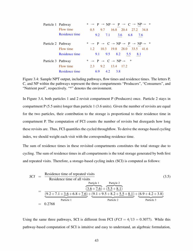
0.5 9.7 16.8 20.4 27.2 34.8

Residence time 9.2 7.1 3.6 6.8 7.6

* *

*

Pathway

Pathway

1.2 10.3 19.8 28.0 33.5 41.6Flow time

Residence time 9.1 9.5 8.2 5.5 8.1

Flow time 2.3 9.2 13.4 17.2

Residence time 6.9 4.2 3.8

Particle 2

*

Pathway *

Flow time

Particle 1

Particle 3

P P

P P

P

C

C

C

NP

NP

NP

NP

NP

Figure 3.4: Sample NPT output, including pathways, flow times and residence times. The letters P,C, and NP within the pathways represent the three compartments “Producers”, “Consumers”, and“Nutrient pool”, respectively. “*” denotes the environment.

In Figure 3.4, both particles 1 and 2 revisit compartment P (Producers) once. Particle 2 stays in

compartment P (5.5 units) longer than particle 1 (3.6 units). Given the number of revisits are equal

for the two particles, their contribution to the storage is proportional to their residence time in

compartment P. The computation of FCI counts the number of revisits but disregards how long

these revisits are. Thus, FCI quantifies the cycled throughflow. To derive the storage-based cycling

index, we should weight each visit with the corresponding residence time.

The sum of residence times in these revisited compartments constitutes the total storage due to

cycling. The sum of residence times in all compartments is the total storage generated by both first

and repeated visits. Therefore, a storage-based cycling index (SCI) is computed as follows:

SCI =Residence time of repeated visits

Residence time of all visits(3.5)

=

Particle 1︷ ︸︸ ︷(3.6+7.6)+

Particle 2︷ ︸︸ ︷(5.5+8.1)

(9.2+7.1+3.6+6.8+7.6)︸ ︷︷ ︸Particle 1

+(9.1+9.5+8.2+5.5+8.1)︸ ︷︷ ︸Particle 2

+(6.9+4.2+3.8)︸ ︷︷ ︸Particle 3

= 0.2768

Using the same three pathways, SCI is different from FCI (FCI = 4/13 = 0.3077). While this

pathway-based computation of SCI is intuitive and easy to understand, an algebraic formulation,

43

which is vastly easier to compute, is also desirable for steady-state networks. As the computation

of FCI (Eq. (3.4)) is in terms of compartmental throughflow T and throughflow matrix N, one

straightforward way to construct SCI formulation is to replace these flow-based terms with the

storage-based terms. Throughflow (T) can be replaced by storage values (x). Ecological Network

Analysis (Fath and Patten, 1999b) provides a storage-based alternative (S) to the throughflow anal-

ysis matrix N, where Si j represents the storage generated at compartment i by per unit input at

compartment j. From the perspective of particles, Si j is the sum of its residence times at i given

that the particle enters the system at j. The algebraic formulation of the storage analysis matrix S

is defined below. Further information on the pathway-based computation and interpretation of S is

provided in Kazanci (2011).

S =−C−1 (3.6)

where

Ci j =

fi j/x j , i 6= j

−Ti/xi , i = j

In the formula of FCI (Eq. (3.4)), by subtracting the first visit, Nii−1 represents the total number

of revisits to compartment i. The corresponding storage-based measures RTi and Sii, respectively,

represent the particles’ residence time at compartment i for the first visit, and the cumulative res-

idence time including all revisits. Then, Sii−RTi, analogous to Nii− 1, is the sum of residence

times of revisits (excluding the first visit). Therefore, (Sii−RTi)/Sii indicates the proportion of

residence time caused by cycling. Based on the algebraic formula of FCI (Eq. (3.4)), simply by

substituting throughflow (Ti) with storage values (xi), and (Nii− 1)/Nii with (Sii−RTi)/Sii, the

SCI formulation that computes the fraction of total system storage (TSS) due to cycling (T SSc) is

proposed as follows:

SCI =T SSc

T SS=

1T SS

n

∑i=1

xiSii−RTi

Sii(3.7)

where TSS (total system storage) is computed as the sum of storage values xi of all compartments in

the system. To further demonstrate that this formula agrees with the pathway-based computation

44

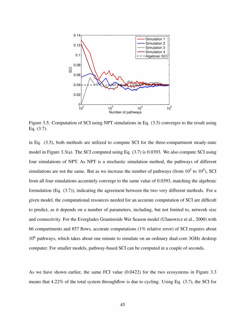
102

103

104

105

0

0.02

0.04

0.06

0.08

0.1

0.12

0.14

Number of pathways

SC

I

Simulation 1

Simulation 2

Simulation 3

Simulation 4

Algebraic SCI

Figure 3.5: Computation of SCI using NPT simulations in Eq. (3.5) converges to the result usingEq. (3.7).

in Eq. (3.5), both methods are utilized to compute SCI for the three-compartment steady-state

model in Figure 3.3(a). The SCI computed using Eq. (3.7) is 0.0393. We also compute SCI using

four simulations of NPT. As NPT is a stochastic simulation method, the pathways of different

simulations are not the same. But as we increase the number of pathways (from 102 to 105), SCI

from all four simulations accurately converge to the same value of 0.0393, matching the algebraic

formulation (Eq. (3.7)), indicating the agreement between the two very different methods. For a

given model, the computational resources needed for an accurate computation of SCI are difficult

to predict, as it depends on a number of parameters, including, but not limited to, network size

and connectivity. For the Everglades Graminoids Wet Season model (Ulanowicz et al., 2000) with

66 compartments and 857 flows, accurate computations (1% relative error) of SCI requires about

106 pathways, which takes about one minute to simulate on an ordinary dual-core 3GHz desktop

computer. For smaller models, pathway-based SCI can be computed in a couple of seconds.

As we have shown earlier, the same FCI value (0.0422) for the two ecosystems in Figure 3.3

means that 4.22% of the total system throughflow is due to cycling. Using Eq. (3.7), the SCI for

45

models (a) and (b) are 0.0393 and 0.0268, respectively, indicating that 3.93% and 2.68% of the

total biomass in system (a) and (b) are due to cycling. Not only the interpretations, but also the

values of FCI and SCI are indeed very different. As the producer in (b) has shorter life span than

that in (a), the turnover rate of producer in (b) is much higher. Therefore, SCI provides potentially

useful information that is not indicated by FCI. For example, assuming that the environmental input

contains pollutants, the lower cycling index in (b) indicates that the system with higher turnover

rate will be affected less by the pollutants.

Based on some equivalent relations between flow rates, storage values, and residence times, an

alternative representation of Eq. (3.7) can be derived. The storage value of a compartment equals

the product of its residence time and throughflow: xi = RTi × Ti. For compartmental models,

a similar relation exists between the storage matrix S and throughflow matrix N: Si j = Ni j×RTi.

Therefore, the term Sii−RTiSii

can be reduced to Nii−1Nii

. Replacing xi with RTi×Ti, SCI can be rewritten

as

SCI =T SSc

T SS=

1∑

ni=1 RTiTi

n

∑i=1

RTiTiNii−1

Nii(3.8)

In this formula, the numerator represents the residence time of recycled throughflow, and the de-

nominator is the residence time of all throughflow. Comparing Eq. (3.4) for FCI and Eq. (3.8) for

SCI, we clearly see that SCI is obtained by weighting FCI with residence times. In other words,

SCI is actually a residence time-weighted FCI. If the residence time is the same for all compart-

ments in the system, the values of FCI and SCI will be the same. However, it is rarely the case in

real ecosystems. Different compartments hold particles for different periods of time. Therefore,

SCI would predict a different impact of recycling than FCI.

Two formulas in Eqs. (3.7) and (3.8) are equivalent and agree with the pathway-based method

for steady-state models. However, ecosystems are rarely at steady state. Flows and storage values

change over time, often fluctuating daily and/or seasonally. Thus, for highly dynamic models,

algebraic formulas of FCI and SCI may not be appropriate. Fortunately, one significant advantage

of pathway-based definitions is their applicability to both steady-state and dynamic models.

46

0 0.2 0.4 0.6 0.80

0.1

0.2

0.3

0.4

0.5

0.6

0.7

0.8

FCI

SC

I

Realistic ecological networks

SCI = FCI

Figure 3.6: SCI vs FCI. Each red star represents a real ecological network in Table 3.1. The bluedashed line indicates SCI = FCI.

3.4 Numerical difference of FCI and SCI

As demonstrated in the last section, both the computation and interpretation of FCI and SCI are

different. Then, another question of interest is how much can FCI and SCI values vary for a

given ecosystem model. To address this issue, we compute SCI and FCI for thirty-six ecological

networks gathered from literature. All of these networks are at steady state. Table 3.1 provides

the reference, and flow currency for each of these ecological networks. The percent difference

between FCI and SCI is computed as the absolute difference between two values, divided by the

average of these two values: FCI−SCI(FCI+SCI)/2 × 100. The column titled “Difference (%)” in Table 3.1

shows that FCI can vastly differ from SCI.

A plot of SCI versus FCI is shown in Figure 3.6. The blue dashed line indicates SCI = FCI. We

observe that SCI can be very different from FCI for most of these models. For example, several

networks at around (0.1, 0.4) have SCI that is almost four times of their FCI. On the other hand,

the network at around (0.2, 0.05) has SCI that is about 1/4 of its FCI.

47

Table 3.1: Comparison of FCI and SCI for thirty-six ecological network models. The percent dif-ference between FCI and SCI is computed as the absolute difference between two values, dividedby the average of these two values: FCI−SCI

(FCI+SCI)/2×100. Connectance is computed as the ratio of thenumber of actual intercompartmental links (d) to the number of possible intercompartmental links:d/(# Compartments)2.

Model Flow

currency

#Comp Connectance FCI SCI Difference

(%)

Lake Oneida (pre-ZM) (Miehls et al., 2009a) Carbon 74 0.221 1.08E-4 5.99E-5 57.29

Lake Oneida (post -ZM) (Miehls et al., 2009a) Carbon 76 0.216 1.34E-4 1.14E-4 16.13

Lake Quinte (pre-ZM) (Miehls et al., 2009b) Carbon 74 0.209 8.78E-4 8.03E-4 8.92

Lake Quinte (post-ZM) (Miehls et al., 2009b) Carbon 80 0.209 0.006 0.011 -58.82

St. Marks Seagrass, site 3 (January) (Baird et al., 1998) Carbon 51 0.048 0.007 0.021 -100.00

Everglades Graminoids Wet Season (Ulanowicz et al., 2000) Carbon 66 0.181 0.018 0.049 -92.54

St. Marks Seagrass, site 4 (February) (Baird et al., 1998) Carbon 51 0.077 0.035 0.086 -84.30

Everglades Graminoids Dry Season (Ulanowicz et al., 2000) Carbon 66 0.181 0.037 0.095 -87.88

Cypress Dry Season (Ulanowicz et al., 1997) Carbon 68 0.120 0.043 0.007 144.00

Cypress Wet Season (Ulanowicz et al., 1997) Carbon 68 0.118 0.044 0.009 132.08

Northern Benguela Upwelling (Heymans and Baird, 2000) Carbon 24 0.201 0.047 0.088 -60.74

Swarkops Estuary (Baird et al., 1991) Carbon 15 0.156 0.056 0.082 -37.68

Ems Estuary (Baird et al., 1991) Carbon 15 0.164 0.059 0.225 -116.90

Crystal Creek (Ulanowicz, 1986b) Carbon 21 0.186 0.066 0.084 -24.00

St. Marks Seagrass, site 2 (February) (Baird et al., 1998) Carbon 51 0.076 0.083 0.208 -85.91

Florida Bay Dry Season (Ulanowicz et al., 1998) Carbon 125 0.126 0.084 0.124 -38.46

St. Marks Seagrass, site 2 (January) (Baird et al., 1998) Carbon 51 0.068 0.086 0.214 -85.33

Crystal River (thermal) (Ulanowicz, 1986b) Carbon 21 0.136 0.090 0.118 -26.92

Mangrove Estuary Wet Season (Ulanowicz et al., 1999) Carbon 94 0.152 0.095 0.049 63.89

Mangrove Estuary Dry Season Ulanowicz et al. (1999) Carbon 94 0.152 0.097 0.049 65.75

St. Marks Seagrass, site 1 (February) (Baird et al., 1998) Carbon 51 0.083 0.109 0.256 -80.55

Oyster Reef (Dame and Patten, 1981) Energy 6 0.333 0.110 0.092 17.82

Neuse Estuary Flow Model, Late Summer 1998 (Baird et al., 2004) Carbon 30 0.093 0.112 0.365 -106.08

Chesapeake Mesohaline Ecosystem (Baird and Ulanowicz., 1989) Carbon 15 0.182 0.116 0.301 -88.73

Neuse Estuary Flow Model, Early Summer 1997 (Baird et al., 2004) Carbon 30 0.088 0.116 0.337 -97.57

Neuse Estuary Flow Model, Early Summer 1998 (Baird et al., 2004) Carbon 30 0.084 0.120 0.349 -97.65

St. Marks Seagrass, site 1 (January) (Baird et al., 1998) Carbon 51 0.075 0.125 0.312 -85.58

Neuse Estuary Flow Model, Late Summer 1997 (Baird et al., 2004) Carbon 30 0.111 0.126 0.365 -97.35

Aggregated Baltic Ecosystem (Wulff and Ulanowicz, 1989) Carbon 15 0.164 0.129 0.211 -48.24

Baltic Sea (Baird et al., 1991) Carbon 15 0.165 0.130 0.221 -51.85

Somme Estuary (Rybarczyk and Nowakowski, 2003) Carbon 9 0.296 0.139 0.204 -37.90

Florida Bay Wet Season (Ulanowicz et al., 1998) Carbon 125 0.124 0.144 0.193 -29.08

Chesapeak Bay Mesohaline Network (Baird and Ulanowicz., 1989) Carbon 36 0.093 0.194 0.066 98.46

Bothnian Bay (Sandberg et al., 2000) Carbon 12 0.201 0.264 0.409 -43.09

Bothnian Sea (Sandberg et al., 2000) Carbon 12 0.215 0.327 0.482 -38.32

Narragansett Bay (Monaco and Ulanowicz, 1997) Carbon 32 0.152 0.505 0.758 -40.06

48

3.5 Compartmental cycling index

While it is often used as a system-wide property, the cycling index can be better characterized

by highlighting the contribution of each compartment. For example, pollutants existing within

an ecosystem may repeatedly visit the same species due to cycling. System-wide cycling indices

quantify the effect of pollution in the system as a whole, but do not provide much information on

how strong the effect of pollution is for each species, or compartment. For such analysis focusing

on single species (or compartment), a compartmental cycling index is more meaningful.

System-wide FCI and SCI are actually computed by summing up the strength of cycling in all

compartments. Their formulations can easily be reduced to represent the strength of cycling for a

single compartment j. For a single compartment j, TST (total system throughflow) is replaced by

the Tj (throughflow at compartment j). Then the FCI for j can be defined as:

FCI j =1

∑i= j

Ti∑i= j

TiNii−1

Nii=

1Tj

TjN j j−1

N j j=

N j j−1N j j

(3.9)

Similarly, SCI (Eq. (3.7)) can be modified to represent compartmental storage-based cycling:

SCI j =1

∑i= j

xi∑i= j

xiSii−RTi

Sii=

1x j

x jS j j−RTj

S j j=

(N j j−1)RTj

N j jRTj=

N j j−1N j j

(3.10)

For steady-state models, residence time (RTj) of an atom, or an energy quantum, is constant for

each compartment j. Once the residence time is out of the equation, compartmental FCI (Eq. (3.9))

and SCI (Eq. (3.10)), although they have different meanings, are numerically equivalent for the

same compartment. For dynamic models, however, the compartmental FCI and SCI values may

differ as they change over time(Kazanci, 2011).

49

3.6 Applications to other systems

So far, our discussion of cycling has been restricted to networks that represent biotic interactions

in the ecosystem. Similar network models are widely used in other areas such as epidemiology,

industry and pharmacokinetics, to represent various interactions among a number of entities of

interest. Naturally the concept of cycling carries different meanings in these areas, such as reinfec-

tion in epidemiology (Gomes et al., 2004), and recycling of materials in industrial systems (Bailey

et al., 2008). Both compartmental and system-wide definitions of cycling indices discussed above

are applicable to networks modeling the flow of some conservative currency. Next, we discuss two

applications: (i) compartmental cycling index in epidemiology; (ii) system-wide cycling index in

industrial system. As these applications are not the primary focus of this paper, we provide a brief

description for each.

In epidemiology, network models are employed to study the transmission of infectious diseases,

where the population of interest is divided into several compartments based on their infection sta-

tus (e.g. susceptible, infected, and recovered) and the flows indicate the transition of infection

status (e.g. infection, recovery, and reinfection). Infectious diseases are often a threat to public

health because of their potential for high transmission among individuals. An important index in

epidemiology is the basic reproduction number (R0) (Fraser et al., 2009), the number of individ-

uals a single infected person will infect on average over the course of its infectious period. Some

diseases, such as the common cold (Wat, 2004), tuberculosis (Verver et al., 2005), and trachoma

(Grayston et al., 1985), may infect individuals multiple times. A reinfection index quantifies the

proportion of infected individuals that are due to reinfection. For such diseases, reinfection index,

in addition to R0, can be potentially useful to evaluate the efficacy of possible strategies utilized

to prevent an epidemic. Figure 3.7 shows a classic SIRS model, where the entire population is

divided into three compartments: S (susceptible), I (infected), and R (recovered). The recovered

individuals might become susceptible after a while, and therefore may get infected again. Comput-

ing reinfection index in this case is equivalent to answering how many of the patients enters I more

50

S I R

Figure 3.7: SIRS model, including three compartments S (susceptible), I (infected) and R (recov-ered). For certain diseases, the recovered individuals may also get reinfected after awhile.

than once. Therefore, the compartmental cycling index in section 3.5 can be utilized to compute a

reinfection index for compartment I.

Certain wasted material such as metal, paper and glass, can be reused to manufacture new prod-

ucts, reducing the usage of raw material. Bailey et al. (2008) have utilized FCI to quantify the

material cycling in industrial systems. As FCI represents the recycled throughflow, it quantifies

the proportion of recycled material used per unit time in production (e.g. the daily yield of a prod-

uct). However, if the focus is the proportion of recycled material currently in use, regardless of its

production date, then the storage-based cycling index SCI serves as the ideal measure.

3.7 Discussion and conclusion

The main contribution of this work is the introduction of a new storage-based cycling index (SCI).

Finn’s original formulation of the cycling index (FCI) has been used by many researchers from a

wide range of disciplines. However, we believe a storage-based cycling index does indeed have a

wide range of potential applications, some of which are mentioned in the previous sections.

SCI has been conceived two decades ago (Patten and Higashi, 1984). However, the cumbersome

formulation using Markov chains hindered its widespread adaptation. In this paper, we provide a

simple algebraic formulation similar to FCI, in addition to a pathway-based formulation that makes

51

this useful but limited formulation applicable to dynamic systems. Many interesting research prob-

lems concern change, therefore the quasi-steady state assumption does not always hold. Studies of

climate change, environmental impacts, regime shifts do need a dynamic formulation.

An interesting point is the vast time difference of over three decades between this manuscript

studying SCI and the original work on FCI by Finn (1976), which makes us wonder why the work

presented in this paper was not published earlier. One reason we anticipate is the inherent difficulty

of utilizing matrix algebra to study and formulate complex system-wide measures involving indi-

rect effects. A recent development, network particle tracking (NPT), has been invaluable tool in

this regard. It is compelling that the pathway-based formulations of cycling, as well as other eco-

logical network analysis measures, which are based on counting arguments applied to the output

of a stochastic individual-based simulation algorithm (NPT), agree with the rather rigid algebraic

formulations. This correspondence, or backwards compatibility, enables us to investigate new

useful formulations of ecosystem measures, using the flexible medium of pathway data, with the

possibility of a corresponding algebraic formulation for easy computation.

While cycling index is originally proposed as a measure for ecological network analysis, the con-

cept of cycling is applicable to, and carries different meanings in other fields, such as reinfection

in epidemiology (Gomes et al., 2004), the reuse of materials in industry (Bailey et al., 2008), and

the recycling of drug within body in parmacokinetics (Hatanaka et al., 1998), to name a few. Our

computation of cycling index for ecosystems is applicable to these areas as well.

52

Chapter 4

How is cycling related to indirect effects in

ecological networks?

4.1 Introduction

Ecological networks are simplifications of complex ecosystems, often used to represent stocks and

flows of conservative quantities (biomass, energy, nutrients) among a set of storage units known

as compartments. Ecological network analysis (ENA) (Hannon, 1973; Patten, 1978; Higashi and

Patten, 1989; Fath and Patten, 1999b) is developed to study the structure and function of ecological

systems based on the idea of economic input-output analysis (Leontief, 1951, 1966). ENA method-

ology formulates various quantitative properties to describe the complex relationships within the

system, such as cycling index (Finn, 1978; Kazanci et al., 2009), throughflow analysis (Matamba

et al., 2009), and indirect effects, to name only a few. The computations of these measures are

often based on complex matrix operations. To enable convenient calculation of these properties,

several computational tools were developed. Fath and Borrett (2006) created a Matlab function to

53

compute the primary network measures. Borrett and Lau (2012) built an R package to implement

a wide range of ENA measures. These two packages work like specific calculators with built-in

formulas of system properties. Given the required data for the network such as boundary inputs

and outputs, inter-compartmental flows, and compartment stocks, these tools calculate and list the

values of various measures. The advantage of these tools is mainly the convenience and efficiency.

However, both tools are only applicable to steady-state networks and are unable to simulate evolv-

ing systems. Similarly, Kazanci (2007) designed a web-based software called EcoNet that offers a

convenient way to both simulate the system and compute ENA measures. EcoNet computes ENA

properties only after the system reaches steady state, and therefore does not actually extend the

applicability of ENA methodology to dynamic systems.

Similar to EcoNet, Network Particle Tracking (NPT) (Kazanci et al., 2009) can simulate ecologi-

cal systems, but offers a new perspective to study ENA measures from a Lagrangian point of view.

NPT discretizes stocks (energy or mass) into small particles, which can be single C atoms, or en-

ergy quanta. This method can trace movements of these particles and stores the path that they flow

through the system. By converting flow rates (boundary inputs, outputs and inter-compartmental

flows) into a list of pathways of particles, NPT can describe the system from the perspective of

the flow material, such as a single C atom, or an energy quantum. The study and formulation of

ENA measures can be based on these pathways and computational algorithms. This is a vastly

different but consistent approach from conventional formula-based packages and software. NPT

has been used to re-investigate, verify and extend the applicability of NEA properties. Kazanci

et al. (2009), Matamba et al. (2009) and Kazanci (2011) show that the NPT methodology and

conventional formula-based computation converge to the same values as for Finn’s cycling index,

throughflow analysis matrix (N), and storage analysis matrix (S), respectively. Ma and Kazanci

(2012a) show that the original definition of indirect effects ratio (I/D) differs from its intended

meaning, and provide a revised formulation. Kazanci (2011) extends ecological network analysis

to dynamic models using storage analysis as an example.

54

Among various system-wide ENA measures, indirect effect index (Patten, 1978) and cycling index

(Finn, 1977, 1978) are perhaps the most widely used. Indirect effects are essential for understand-

ing how ecosystems function. Krivtsov (2004, 2009) believes systematic elucidation of indirect

effects is becoming central for ecology and environmental science. Min et al. (2011) states that

indirect effects are assumed to be the major causes of the complexity and stability of ecological

networks. Wootton (2002) claims that indirect effects cause the challenge to predict the of impacts

of environmental change. Thus, a better understanding of indirect effects seems critical to under-

stand and predict ecosystem behavior. Similarly, cycling index is an essential ecological indicator

for ecosystem analysis. It measures how much of the environmental input into the system is cycled

before exiting the system. According to Odum (1969), cycling is an indicator of system maturity.

Cycling of carbon, however, can be a sign of a more stressed community, and appears to be a

counter-indicator of ecosystem health (Wulff and Ulanowicz, 1989). A widely accepted method

for quantifying cycling for ecosystem models is Finn’s cycling index (FCI) (Finn, 1978), which

calculates the fraction of throughflow generated by cycling over the total system throughflow.

Fath (2004), using a set of large-scale cyber-networks, observes a strong correlation exists between

indirect effects index and cycling index. Strong correlation doesn’t establish a causal relationship

between two variables. Further questions regarding this close relation remain unanswered. For ex-

ample, does cycling indeed increase indirect effects? We know that an ecological network without

cycling still retains indirect effects, which indicates that indirect effects might be partially boosted

by the cycling in the network. Then perhaps indirect effects index is a composite measure, involv-

ing some parts that are highly related to cycling, as well as some that are independent of cycling. In

this chapter, we investigate the relation between indirect effects and cycling in detail, and decom-

pose indirect effects into three disjoint components based on their relation to cycling and direct

effects.

55

4.2 Indirect effects and cycling

4.2.1 Definitions of IEI and FCI

Ecosystems are often modeled as compartmental systems, where active members in the ecosystem

are categorized into compartments, and transactions of specific currencies among compartments

are identified and measured. Total effects in the system represent all relations among all compart-

ments. Depending on whether the effects between two compartments are transmitted via others,

effects are classified into two categories: direct and indirect. The I/D ratio is defined to represent

the ratio of indirect to direct effects. An indirects effect index (IEI), computed as I/(I +D), rep-

resents the proportion of indirect to total effects (Ma and Kazanci, 2012a). To quantify cycling,

total system throughflow is divided into two parts: flows generated by first visits, and flows gener-

ated through cycling. The proportion of this second part is defined as Finn’s cycling index (FCI).

Computation of IEI and FCI relies on the flow information in the ecological system:

zi : Rate of environmental input to compartment i

yi : Rate of environmental output from compartment i

Fi j : Rate of direct flow from compartment j (columns of F) to compartment i (rows of F)

Throughflow Ti is the rate of material (or energy) moving through compartment i. Input through-

flow is defined as the sum of flow rates into compartment i from other compartments and the

environment. Similarly, output throughflow is the sum of flow rates from compartment i to other

compartments and the environment. For a system at steady state, input and output throughflows

are equal to each other.

Ti =n

∑j=1

Fi j + zi =n

∑j=1

Fji + yi

56

where n represents the number of compartments in the system. Total system throughflow (TST) is

the sum of all throughflows in the system. The flow intensity matrix G is obtained by normalizing

the rows of the flow matrix F by the throughflow vector T :

Gi j =Fi j

Tj

G is actually a one-step probability transition matrix, Gi j is the fraction of the flow material orig-

inating from j and moving to i directly ( j → i). Therefore by definition, Gi j ≤ 1 for all i, j.

Similarly, [G2]i j is the the fraction of the flow moving to j from i over two steps ( j→ k→ i). In

general, [Gm]i j represents the fraction of the flow material from j to i over m steps ( j→ ··· → i︸ ︷︷ ︸m

).

The infinite sum of all powers of the G matrix defines the throughflow analysis matrix N:

N = I︸︷︷︸Boundary

+ G︸︷︷︸Direct

+ G2 +G3 + · · ·︸ ︷︷ ︸Indirect

= (I−G)−1 (4.1)

where I is the identity matrix, not to be confused with the I used later to denote the indirect effects.

Ni j represents the throughflow generated at compartment i by per unit input at compartment j.

Patten (1978) defines the ratio of indirect to direct flow (I/D) as a measure to quantify the effect of

indirect relations among compartments relative to direct connections.

(ID

)unit

=

n∑

i=1

n∑j=1

(G2 +G3 + . . .)

n∑

i=1

n∑j=1

G=

n∑

i=1

[(N− I−G)~1

]n∑

i=1(G~1)

(4.2)

where~1 is a vector of ones. Ma and Kazanci (2012a) find out the Eq. (4.2) compares indirect and

direct flows generated by unit throughflows at all compartments, but not by the actual throughflows.

Therefore a revised formulation for I/D is proposed as follows:

(ID

)revised

=

n∑

i=1

[(G2 +G3 + · · ·)T

]n∑

i=1(GT )

(4.3)

57

I/D ratio can take any value from zero to infinity. Zero implies that no indirect effects exist. Direct

effects equal indirect effects if I/D= 1. Dominance of indirect effects holds if 1< I/D<∞. Direct

effects dominate if 0 < I/D < 1. The interval of values where dominance of indirect hypothesis

holds is of length infinity, where as the interval of values where direct effects dominate is of length

1. To eliminate this imbalance, Ma and Kazanci (2012a) defines the Indirect Effects Index (IEI),

which is derived by rescaling the I/D ratio as follows:

IEI =I

I +D=

( ID

)1+( I

D

) (4.4)

IEI acts much like FCI, with a range between zero and one. For an ecological network, IEI =

0, 0.5 and 1 imply no indirect effects, equal amount of direct and indirect effects, and no direct

effects, respectively. Note that IEI can never be equal to one, though can be arbitrarily close to

one.

The computation of FCI depends on the throughflow analysis matrix N, as well. By definition,

diagonal values of Nii represent the amount of throughflow generated at compartment i by one unit

input into compartment i. A unit input into compartment i contributes to its throughflow (Ti) at

least once. Therefore, if Nii is larger than 1, then the difference Nii− 1 represents the amount of

throughflow generated at compartment i through cycling. Finn (1978) defines his cycling index

based on this idea, as the fraction of the total system throughflow (T ST ) that is due to cycling

(T STc), as follows:

FCI = T STcT ST =

1T ST

n

∑i=1

(Ti

Nii−1Nii

)(4.5)

4.2.2 Comparison of IEI and FCI

For an accurate statistical comparison of IEI and FCI, we use both artificial and real ecological

networks. In this section, we first check the correlation between IEI and FCI using a set of con-

58

ceptual networks. To accomplish this, we generated 100,000 conceptual models, representing all

possible networks with up to five compartments, as shown in Figure 4.1. A compromising number

five is chosen as the network size, mainly because of the heavy computation required to study a

wide range of flow values. While there are usually three to five trophic levels in an ecosystem, our

conceptual model is able to represent an ecosystem with up to five trophic levels, thus is not too

simple.

To build such 100,000 conceptual models, we initially define a fully connected five-compartment

network, which has the potential to represent any network at steady-state with up to five compart-

ments. We then assign flow rates ranging from zero to 105, individually for each flow, environmen-

tal input and output, while making sure the system is at steady-state. Assigning zero flow rates is

effectively deleting flows, creating sub-networks with simpler structures. Similarly, if all flow rates

in and out of a specific compartment happen to be zero, then the resulting network will represent

models with only four compartments. Therefore, by randomizing flow rates in this fully connected

five-compartment model, it is theoretically possible to generate all possible networks of up to five

compartments.

While the set of all networks with up to five compartments has infinite elements, we set our range

so that any steady-state network with less than six compartments is very close (exactly the same

in terms of structure, and very similar in terms of flow rates) to one of the 100,000 networks we

generated. Therefore, although a fully connected network such as the one shown in Figure 4.1 is

not a realistic representation of an actual ecosystem, it is guaranteed that any ecological network

with up to five compartments is closely represented in our sample set of 100,000 networks.

We then compute IEI and FCI for each of the 100,000 elements of our sample network set. Figure

4.2 shows a scatter plot of IEI and FCI for all networks. We find it striking that regardless of the

network structure (topology) and flow rate values, an extremely strong correlation between FCI

59

A B

C

D

E

Figure 4.1: A fully connected five-compartment network. Each compartment has both an environ-mental input and output, and is connected to all other compartments. By randomizing flow rates inthis fully connected five-compartment model, it is theoretically possible to generate all networkswith up to five compartments.

0 0.2 0.4 0.6 0.8 10

0.2

0.4

0.6

0.8

1

FCI

IEI

Figure 4.2: Relationship between IEI and FCI of 100,000 conceptual networks representing allpossible steady-state ecological networks with up to five-compartments. Each gray dot representsa single model.

60

and IEI is observed, even for unrealistic networks. As FCI increases, the variation of IEI decreases

dramatically. For non-cycling networks (FCI = 0), IEI ranges between zero and 0.6. However, for

networks with 80% cycling (FCI = 0.8), IEI can be estimated to be 0.9 with very little error. This

experiment confirms the strong correlation between IEI and FCI. However, the vertical spread of

data, i.e., the high variation of IEI especially for small FCI values, requires further attention.

Our preliminary result is based on a set of conceptual networks of up to five compartments, most of

which are probably unrealistic. This observation may not hold for real ecological networks, which

may have a higher number of compartments and connections, and be more complex in general. In

order to check if our observations extend to real life cases, we compute the IEI and FCI of thirty

real ecosystem models selected from the literature, with number of compartments ranging from 4

to 125. Table 4.1 provides the detailed information for each model used in this analysis, including

references. By superimposing the scatter plot of IEI vs. FCI for these thirty ecosystem models

onto Figure 4.2, we get Figure 4.3. As all thirty ecological networks have FCI values lower than

0.35, we only show the scatter plot for FCI between 0 to 0.35.

Figure 4.3 shows that real and conceptual ecological network models show pretty consistent results

for IEI vs FCI, despite the fact that most of the conceptual models are actually unrealistic, and that

some real ecosystem models are a lot larger and more complex. Combining real models with a

high number of conceptual networks enables us to reach a more general conclusion on this special

relationship between IEI and FCI, which transcends the model structure, flow type and network

size. There has to be a universal rule governing this interesting relation between IEI and FCI that

also explains the change in the variation IEI between high and low FCI values.

61

Tabl

e4.

1:T

hirt

yec

olog

ical

netw

ork

mod

els

from

liter

atur

eM

odel

Flow

curr

ency

#of

com

part

men

tsFC

IIE

IIE

I-cy

cle

IEI-

mix

edIE

I-pu

re

Nor

thSe

a(S

teel

e,19

74)

Ene

rgy

100

0.38

10

00.

381

Silv

erSp

ring

s(O

dum

,195

7)E

nerg

y5

00.

151

00

0.15

1

Eng

lish

Cha

nnel

(Bry

linsk

y,19

72)

Ene

rgy

60

0.24

50

00.

245

Lak

eO

neid

a(p

re-Z

M)(

Mie

hls

etal

.,20

09a)

Car

bon

741.

08E

-40.

190

2.14

E-4

2.19

E-4

0.19

0

Lak

eO

neid

a(p

ost-

ZM

)(M

iehl

set

al.,

2009

a)C

arbo

n80

1.34

E-4

0.29

22.

03E

-42.

18E

-40.

291

Lak

eQ

uint

e(p

re-Z

M)(

Mie

hls

etal

.,20

09b)

Car

bon

748.

78E

-40.

182

2.09

E-3

1.85

E-3

0.17

8

Lak

eQ

uint

e(p

ost-

ZM

)(M

iehl

set

al.,

2009

b)C

arbo

n80

0.00

610.

228

0.01

08.

91E

-30.

209

Eve

rgla

des

Gra

min

oids

Wet

Seas

on(U

lano

wic

zet

al.,

2000

)C

arbo

n66

0.01

80.

412

0.02

10.

021

0.36

9

Cyp

ress

Dry

Seas

on(U

lano

wic

zet

al.,

1997

)C

arbo

n68

0.04

30.

423

0.06

30.

077

0.28

3

Cyp

ress

Wet

Seas

on(U

lano

wic

zet

al.,

1997

)C

arbo

n68

0.04

40.

415

0.06

90.

085

0.26

1

Eve

rgla

des

Gra

min

oids

Dry

Seas

on(U

lano

wic

zet

al.,

2000

)C

arbo

n66

0.04

60.

473

0.03

90.

042

0.39

1

Nor

ther

nB

engu

ela

Upw

ellin

g(H

eym

ans

and

Bai

rd,2

000)

Car

bon

240.

047

0.46

80.

039

0.04

00.

382

Cry

stal

Cre

ek(U

lano

wic

z,19

86b)

Car

bon

210.

066

0.39

10.

094

0.09

90.

199

Flor

ida

Bay

Trop

hic

Exc

hang

eM

atri

x(U

lano

wic

zet

al.,

1998

)C

arbo

n12

50.

084

0.54

50.

065

0.08

70.

392

Con

eSp

ring

(Till

y,19

68)

Ene

rgy

50.

092

0.46

20.

096

0.11

00.

256

Man

grov

eE

stua

ryW

etSe

ason

(Ula

now

icz

etal

.,19

99)

Car

bon

940.

095

0.60

30.

091

0.11

90.

393

Man

grov

eE

stua

ryD

rySe

ason

(Ula

now

icz

etal

.,19

99)

Car

bon

940.

097

0.60

40.

091

0.11

80.

394

Oys

terR

eef(

Dam

ean

dPa

tten,

1981

)E

nerg

y6

0.11

00.

593

0.11

80.

158

0.31

7

Che

sape

ake

Mes

ohal

ine

Eco

syst

em(B

aird

and

Ula

now

icz.

,198

9)C

arbo

n15

0.11

60.

597

0.10

50.

118

0.37

4

Agg

rega

ted

Bal

ticE

cosy

stem

(Wul

ffan

dU

lano

wic

z,19

89)

Car

bon

150.

129

0.63

90.

090

0.11

60.

432

Som

me

Est

uary

(Ryb

arcz

ykan

dN

owak

owsk

i,20

03)

Car

bon

90.

139

0.46

00.

167

0.15

00.

143

Flor

ida

Bay

Wet

Seas

on(U

lano

wic

zet

al.,

1998

)C

arbo

n12

50.

144

0.62

00.

102

0.13

20.

385

Cha

rca

Lag

oon

(Alm

unia

etal

.,19

99)

Car

bon

210.

182

0.73

50.

112

0.15

30.

470

Che

sape

akB

ayM

esoh

alin

eN

etw

ork

(Bai

rdan

dU

lano

wic

z.,1

989)

Car

bon

360.

194

0.73

10.

123

0.15

20.

456

Yth

anE

stua

ry(B

aird

and

Miln

e,19

81)

Car

bon

130.

225

0.66

10.

171

0.18

30.

307

Bot

hnia

nB

ay(S

andb

erg

etal

.,20

00)

Car

bon

120.

264

0.73

20.

142

0.16

60.

424

Lak

eFi

ndle

y(R

iche

yet

al.,

1978

)C

arbo

n4

0.29

50.

665

0.32

00.

270

0.07

6

Mir

rorL

ake

(Ric

hey

etal

.,19

78)

Car

bon

50.

308

0.68

80.

293

0.28

40.

110

Mar

ion

Lak

e(R

iche

yet

al.,

1978

)C

arbo

n5

0.30

90.

705

0.28

80.

292

0.12

5

Bot

hnia

nSe

a(S

andb

erg

etal

.,20

00)

Car

bon

120.

327

0.75

50.

210

0.23

90.

306

62

0 0.1 0.2 0.30

0.1

0.2

0.3

0.4

0.5

0.6

0.7

0.8

FCI

IEI

Figure 4.3: Relationship between IEI and FCI for thirty real ecosystem models from Table 4.1(black dots), and 100,000 conceptual networks with up to five compartments (gray dots).

4.3 Decomposing indirect effects

The high correlation between these two different properties indicate that they quantify a similar

attribute of the network, but the variability of IEI reveals that IEI involves an attribute that is

independent of cycling. Unfortunately, neither the statistical analyses, nor the complex algebraic

definitions of IEI and FCI offer any further information that explain the reasons for this relationship

between the two measures. Therefore we need to employ alternative methods to get more useful

insights into the interplay between cycling and indirect effects.

From a network point of view, IEI represents the proportion of total connections that are not adja-

cent. The transfer of mass or energy from compartment i to j is defined as direct effects only if it

occurs between two adjacent compartments through a direct flow i→ j. Otherwise it is classified

as indirect effects if other compartments are involved in this transfer (e.g. i→ k→ j). Figure 4.4

shows three different cases of indirect effects from i to j where two compartments are connected

through a single path. The figure also depicts the network representation of each pathway, where

all compartments are listed without repetition and are connected by directed links. All three cases

63

Figure 4.4: Three types of indirect effects from compartment i to j, presented in the form of apathway and a network. j = i for (a).

are classified as indirect effects as defined by Eq. 4.3. From the perspective of the network, we can

clearly see the involvement of cycling. For example, Figure 4.4(a) shows the indirect effect of i on

itself, which is actually a simple cycle. This type of indirect effect depends exclusively on cycling.

Figure 4.4(b) shows a second type of indirect effect of i on j, which is actually a simple cycle at i

combined with a direct effect of i on j. This second type of indirect effect also depends on cycling,

but interestingly on the direct effect (i→ j) as well. Therefore if the existing direct link from i to j is

broken, this indirect effect will disappear as well. This is somewhat contrary to the understanding

that indirect effects help increase robustness, resilience and potentially stability, as the flow of

biomass and energy from one compartment to another can occur through multiple routes. For a

system with high indirect effects, removing a flow will probably have less impact (e.g. extinction

of a species) due to the existence of multiple independent pathways among compartments will help

the system continue to function as usual. However, this type of indirect effect will not contribute to

such quality. Figure 4.4(c) represents a third type of indirect effect of i on j, which is independent

of both cycling and direct effects. Since i and j are only connected through other compartments, a

broken direct link from i to j will not eliminate this an indirect effect.

64

Based on the three examples on Figure 4.4, we define three types of indirect effects:

(a) IEI-cycle: i→ ··· → i

(b) IEI-mixed: i→ ··· → j contains the direct flow i→ j, (i 6= j)

(c) IEI-pure: i→ ··· → j does not contain the direct flow i→ j, (i 6= j)

IEI-cycle is simple cycle from a compartment to itself, involving one or more other compartment(s)

in between. IEI-mixed represents the indirect effect between compartments that also depends on

the direct effect between the same two compartments. By definition, IEI-mixed has to contain

a cycle within itself as well. IEI-mixed does not seem to contribute to network robustness or

resilience, as its existence entirely depends on the direct effect. IEI-pure is independent of the

direct effect, and is probably a key contributor to network resilience and stability. These three

types of indirect effects are mutually disjoint and their sum constitute the total indirect effects

index (IEI):

IEI = IEI-cycle+ IEI-mixed+ IEI-pure

The existence of both IEI-cycle and IEI-mixed depends on cycling, as they involve cycles (repeated

nodes) in their pathway. If FCI = 0, then IEI-mixed = IEI-cycle = 0. On the other hand, IEI-pure

does not require a repeated node in its pathway, but this does not preclude cycles. For example,

the path i→ m→ n→ m→ j satisfies our criteria for IEI-pure from i to j. However, the value of

IEI-pure is still going to be positive even if FCI = 0.

To compute the three components of IEI individually, we need all possible paths of material flow

through the system. An agent-based stochastic simulation method called Network Particle Track-

ing (NPT) (Kazanci and Ma, 2012) is used for this purpose. NPT discretizes the stocks into parti-

cles, as shown in Figure 4.5. Then, NPT uses probabilities based on the flow values to move the

particles between compartments. The movement of each particle in the system is traced and the

path of each particle is recorded.

65

34 123 421234

156

2

91

236

111

321 122 46 17

19 44

69 731121

New particles from

the environmentInput from

the environment

(1) (2)

(3)

4312

57 717

212

many more ...46

22

Producers

Producers Consumers

Nutrient pool

Nutrient pool

Consumers

Entered Nutrient pool at time =124.6 units.

Passport of Particle 12

Entered Producers at time = 21.2 units.

Moved to Consumers at time = 34.5 units.

Left Nutrient pool at time = 139.7 units.

Figure 4.5: Network Particle Tracking (NPT) discretizes compartmental stocks into particles. Themovement of each particle in the system is traced and recorded. The passport of particle 12 isshown as an example.

The pathway that a particle goes through the system is recorded as a list of ordered compart-

ment numbers. For example, in the three-compartment system in Figure 4.5, numbers 1, 2 and 3

represent Producers, Consumers, and Nutrient Pool, respectively. Figure 4.6 shows one possible

pathway that a particle moves through this system. Ma and Kazanci (2012a) compute IEI using

pathways, and shows that the pathway-based computation agrees with the algebraic formula (4.4).

The pathway-based IEI is simply computed as the proportion of dashed arrows over the total num-

ber of solid plus dashed arrows. Note that the environmental inputs (e.g. ∗ → 1) and outputs (e.g.

3→∗) arrows are not counted because they do not represent within-system interactions.

For a real ecological network, NPT simulation generates a long list of pathways that particles

move through the system. By decomposing all the indirect relations within each pathway, we

can quantify the three components of IEI for the entire system. For the single pathway shown in

Figure 4.6, there are totally four direct connections, and six indirect connections (three 2-step, two

66

2 steps

4 steps

3 steps

* 1 3 1 2 3 *

Figure 4.6: One pathway from NPT simulation of the three-compartment system in Figure 4.5. “∗”represents the environment. Black arrows represent the direct flows in the system. Dashed arrowsare the indirect flows.

Table 4.2: Calculation of direct effects and three types of indirect effects (IEI-cycle, IEI-mixed andIEI-pure)

Classification of effects All connections Counts Proportion (index value)

Direct effect

1-step: 1→ 3

4 0.41-step: 3→ 11-step: 1→ 21-step: 2→ 3

IEI-cycle2-step: 1→ 3→ 1

2 0.23-step: 3→ 1→ 2→ 3

IEI-mixed3-step: 1→ 3→ 1→ 2

2 0.24-step: 1→ 3→ 1→ 2→ 3

IEI-pure2-step: 3→ 1→ 2

2 0.22-step: 1→ 2→ 3

Total 10 1

3-step and a single 4-step). The classification of all these connections as IEI-cycle, IEI-mixed and

IEI-pure is shown in Table 4.2.

Using the algorithm shown in Table 4.2, we first use NPT to simulate the thirty real ecosystem

models provided in Table 4.1 and then compute IEI-cycle, IEI-mixed and IEI-pure for each net-

work. Figure 4.7 shows the comparison of each IEI component with respect to FCI.

Figure 4.7 shows that both IEI-cycle and IEI-mixed increase with the growth of FCI in a linear

fashion (R = 0.9373 and R = 0.9603, respectively). What we consider as “pure indirect effects”,

IEI-pure, is totally unrelated to FCI (R = -0.0870). These results explain our previous observation

67

0 0.05 0.1 0.15 0.2 0.25 0.3 0.350

0.05

0.1

0.15

0.2

0.25

0.3

0.35

FCI

IEI−

cycle

(a)

R = 0.9373; P−value < 0.0001

0 0.05 0.1 0.15 0.2 0.25 0.3 0.350

0.05

0.1

0.15

0.2

0.25

0.3

0.35

FCI

IEI−

mix

ed

(b)

R = 0.9603; P−value < 0.0001

0 0.05 0.1 0.15 0.2 0.25 0.3 0.350

0.1

0.2

0.3

0.4

0.5

FCI

IEI−

pure

(c)

R = −0.0870; P−value = 0.6476

Figure 4.7: Relationship between three indirect effect components (IEI-cycle, IEI-pure, IEI-mixed)and FCI. R represents the Pearson correlation coefficient, indicating the strength of a linear rela-tionship between two variables. The higher the |R|, the stronger the correlation. R values that areclose to zero indicate the two variables are uncorrelated. P-values refer to the probability that theresults of a data analysis are purely random. Smaller P-values indicate a strong predictive rela-tionship. By convention, if the P-value is less than 0.05, the correlation is said to be statisticallysignificant.

68

that IEI and FCI are strongly correlated for high cycling networks, whereas more variation of IEI

is observed for low cycling networks. For high cycling networks, both IEI-cycle and IEI-mixed

dominate IEI-pure, and leave little room for variation of IEI with respect to FCI. On the other hand,

for low cycling networks, IEI-pure becomes the dominating component of IEI. Since IEI-pure is

not correlated to FCI, we observe a high variation of IEI when FCI is small.

4.4 Statistical prediction of IEI-pure using IEI and FCI

As we do not have a closed algebraic formula for each component of IEI, decomposition of IEI is

not easily calculated without computer simulations. Yet a good approximation is possible based on

the fact that the two components of IEI are strongly correlated with FCI. By fitting a line to the data

set, we can predict IEI-cycle (IEI-cycle = 0.8313×FCI) and IEI-mixed (IEI-Mixed = 0.8835×FCI).

Then we can estimate IEI-pure as follows:

Predicted IEI-pure = IEI− (0.8313+0.8835)×FCI (4.6)

Figure 4.8 shows the accuracy of this estimation by comparing the predicted and actual IEI-pure.

4.5 Discussion

In this chapter, we investigate the close relationship between two important ecological network

measures, cycling (FCI) and indirect effects (IEI) in detail. Both FCI and IEI have a simpler

69

0 0.1 0.2 0.3 0.4 0.50

0.1

0.2

0.3

0.4

0.5

IEI Pure

Pre

dic

ted

IE

I P

ure

Figure 4.8: Predicted IEI-pure (4.6) vs actual IEI-pure

and more intuitive description within the context of pathways, compared to their algebraic for-

mulations. Therefore we utilize a pathway-based method to decompose IEI into three disjoint

components (IEI-cycle, IEI-mixed and IEI-pure), based on their relation to cycling.

Eliminating the influence of cycling on indirect effect results in IEI-pure. An essential feature of

IEI-pure is its independence of not only cycling, but also direct effects. While IEI is a mathemat-

ically well-defined index, its practical implications on ecosystem function are not well-studied.

Min et al. (2011) claims that indirect effects can be the major causes of the stability of ecological

networks. However, we feel that not every component of IEI contributes to stability or resilience

equally. A high value for IEI-mixed may be less important than a lower value for IEI-pure within

the context of ecosystem resilience. Further research is needed to understand the practical im-

plications of indirect effects, which may lead to a more appropriate formulation based on a new

context.

In contrast to the strong correlation between IEI and FCI, we observe almost no correlation between

IEI-pure and FCI. Therefore, while IEI and FCI combines similar attributes of an ecosystem model,

IEI-pure and FCI quantifies completely different aspects of ecosystem function, which may be

more desirable for some applications. For example, if multiple ENA measures are used to compare

two different networks, then we already know that IEI and FCI will show similar results with a high

70

probability. On the other hand, IEI-pure and FCI are capable to capture quasi-orthogonal attributes

of the system, which, potentially can be more informative.

A significant disadvantage of IEI-pure is the need for a simulation for accurate computation. Nev-

ertheless, it is possible to construct a somewhat decent approximation for IEI-pure based on FCI

and IEI. This work does not only explain the correlation between cycling and indirect effects ob-

served in earlier work, but also reveals an index that may be better suited to quantify the indirect

relations in ecosystems that contribute to stability, robustness and resilience.

71

Chapter 5

A comparison of system-wide measures in

ecological network analysis

5.1 Introduction

In the last three decades, it has been gaining in popularity to study the ecosystem as a whole unit

rather by isolating and focusing on each individual species independently. Even though the tar-

get is individual species, it is vital to study its behavior as embedded in a larger system. To date,

simulation modeling has been the most common tool for quantifying system-level events (Ulanow-

icz, 2004). Ecological network analysis (ENA) (Patten, 1978; Fath and Patten, 1999b; Ulanowicz,

2004) is a system-oriented methodology to simulate and analyze within-system interactions. This

method is an extended application of economic input-output analysis (Leontief, 1966), which is

first introduced to ecology by Hannon (1973). Compartmental models are constructed to repre-

sent the transactions of energy/matter in ecosystems. To facilitate the evaluation of the ecosystem,

various system-wide measures have been proposed to capture the holistic properties, or the sys-

72

tem characteristics of a focal ecosystem (Jørgensen et al., 2013). Over the years, ENA has been

enriched by the development of new ecological measures, as well as the transfer of network mea-

sures from other fields. Finn’s cycling index (FCI) (Finn, 1977) is based on the Leontief structure

matrix (or throughflow matrix), initially developed for economic input-output analysis (Leontief,

1966). Ascendancy and several related measures (Ulanowicz, 1986b) are based on information

theory (MacArthur, 1955; Rutledge et al., 1976). These system-wide measures play an increas-

ingly important role in studying and assessing various ecosystems (Patrício et al., 2004), including

forest ecosystems (Schaubroeck et al., 2012), marine ecosystems (Tomczak et al., 2013) and lake

ecosystems (Chrystal and Scharler, 2014).

Unlike empirical ecological indicators (e.g., the concentration of a toxic substance, and primary

production rate), system-wide measures are often defined based on compartmental models of the

ecosystems, and may have complex computations. Except several basic measures (e.g., #links,

#compartments, and total system throughflow), most of these measures (e.g., FCI, ascendency, and

development capacity) usually require a more profound understanding of which health aspects they

are able to cover and how they can be used in environmental management (Jorgensen et al., 2005).

This causes difficulties for every user to comprehensively understand, compute and interpret all

measures. Our project is aimed to advance our understanding of system-wide ecological measures

by studying the relationships among them.

Our project is not the first attempt to investigate the relationship of different measures. Studies of

pairwise relationships have been conducted through theoretical and empirical investigations. Co-

hen and Briand (1984) reports that the link density (the average number of links per compartment)

does not change with network size. In contrast, Havens (1992) shows link density increases with

network size. The relationship between connectance (the proportion of possible links between

compartments that are realized) and network size has also been studied. Yodzis (1980) finds a

somewhat slow decrease of connectance with increasing species richness, while Martinez (1992)

reports that the connectance tends to remain constant across networks of different size. Higashi

73

and Patten (1986, 1989) and Patten (1991) show that indirect effects increase with network size,

connectance, FCI and total system throughflow.

In addition, Fath (2004) develops an algorithm to construct large-scale cyber-ecosystems and in-

vestigates how four system-wide measures (amplification, homogenization, synergism and indi-

rect effects) change with network size. Fath classifies all compartments into six functional groups:

primary producers, grazers, omnivores, carnivores, detrital feeders, and detritus. To construct a

network, the same number of compartments is chosen from each group. Then, connections are

established among compartments based on three assumptions, for which Fath (2004) provides a

detailed explanation. Finally, flow values are assigned using randomly selected transfer efficiency

coefficients and then back calculate the flows. However, the detail on assigning flow values is not

given in the paper. Using this algorithm, Fath (2004) constructs networks of five different sizes:

30, 60, 120, 300, and 600 compartments. Based on these generated networks, he finds out that

amplification only occurs sparingly in smaller networks, synergism always occurs but decreases as

network size increases, and homogenization and indirect effects increase with network size. Al-

though these “cyber networks” are constructed based on seemingly reasonable assumptions, there

is little evidence that as a set, these networks accurately represent real ecosystems. For example,

we observe that FCI (Finn, 1976) changes over a rather narrow range from 0.14 to 0.25 for these

networks. Theoretically, FCI can be [0, 1). It is known that many ecosystem models from litera-

ture have FCI values outside of this narrow range. For example, all sixteen seasonal nitrogen flow

models of Neuse River estuary (Christian and Thomas, 2003) have FCI around 0.9. Thus, these

generated networks may not be good representatives of all possible real ecosystems. As additional

information (e.g. network structure, flow rates, and storage values) about these networks is not

provided in the paper, it is hard to further evaluate how well these networks represent the real

ecosystems.

The above studies mainly focus on the relationship of pairwise measures. Buzhdygan et al. (2012)

compares ten system-wide measures for seven geographically close pastoral ecosystems. The con-

nections are built based on three years of field research. However, flow and storage values are

74

assigned using simple rules. Boundary inputs and standing stocks are assigned values of one. All

the flows leaving a compartment i have equally distributed flow rates: 1/(the number of flows leav-

ing i). Then these networks are simulated in EcoNet (Kazanci, 2007) to reach steady states. Ten

system-wide measures (connectance, link density, total system throughflow, FCI, ascendency, de-

velopment capacity, indirect effects, system aggradation, system synergism, and mutualism) com-

puted by EcoNet are compared. Except connectance and link density, all the other eight measures

are defined using the flow values of the ecosystem. However, the flow and storage values in these

seven pastoral networks are not based on field work, and therefore are not realistic. For example,

the storage values are all set to be ones, which is unlikely to occur in real ecosystems. It is also

highly unlikely that all compartments have equal environmental inputs. In addition, the flow rates

leaving a compartment are often not equally distributed among all the exiting links.

These previous works on the relationships of measures usually only focus on a few widely used

measures, or are based on unrealistic or incomplete networks. A thorough search of the literature

informs us that there exist forty, or perhaps even more system-wide measures. Nine of these

measures are based on the topology (adjacency matrix) of the network, twenty-six are defined using

flow rates, and five are based on storage information. In this project, we perform a comprehensive

comparison of forty system-wide measures (1) to gain a better understanding of the relationships

among these system-wide measures; (2) to identify and investigate any unexpected relationships

among them; and (3) to compare three major groups of measures: structure-based, flow-based and

storage-based.

Due to complex formulations and computations, the mathematical relations of these measures

cannot properly be described in an algebraic fashion. This study is performed based on published

network models of fifty-two ecosystems, with a variety of network sizes, flow currencies, flow

and storage magnitudes. A useful statistical method called cluster analysis is applied to study the

relations of forty measures, and to classify them based on their similarities. We report our findings

and compare them with observations from earlier published works.

75

5.2 Ecological network analysis (ENA) and system-wide mea-

sures

ENA works with the representations of ecosystems as compartmental models. Compartments rep-

resent various entities in the ecosystem, such as plants, animals, and nutrient sources. The flows

among compartments are the transport of energy/matter within the system. Boundary input and

output represent the transfer of energy/matter between the system and the outside. Each model

contains the following data: environmental inputs (z), environmental outputs (y), flow matrix (F)

and storage value (x). Assuming there are n compartments in the system, all flows and storages are

denoted as follows:

zi : Rate of environmental input to compartment i

yi : Rate of environmental output from compartment i

xi : Storage value at compartment i

Ai j : Indicator of flow from compartmentent j (columns of A) to compartment i (rows of A)

Fi j : Rate of direct flow from compartment j (columns of F) to compartment i (rows of F)

where i, j = 1, 2, · · · , n. We also define a generalized flow matrix (GF), which includes the inter-

compartmental flows, environmental input and environmental output. GFi j (i, j = 1, 2, · · · , n+1)

represents the rate of direct flow from compartment/the environment j (columns of GF) to the

compartment/the environment i (rows of GF).

GF =

F z

y 0

Utilizing the above scheme, several other useful quantities are also computed. Throughflow Ti is

the rate of material (or energy) moving through compartment i. Input throughflow is defined as the

76

sum of flow rates into compartment i from other compartments and the environment. Similarly,

output throughflow is the sum of flow rates from compartment i to other compartments and the

environment. For a system at steady state, input and output throughflows are equal:

Ti =n

∑j=1

Fi j + zi =n

∑j=1

Fji + yi

Flow intensity matrix G is obtained by normalizing the flow matrix F by the throughflow T :

Gi j =Fi j

Tj

G is actually a one-step probability transition matrix, where Gi j represents the probability of tran-

sitioning from compartment j to compartment i in one step. [Gm]i j represents the fraction of the

flow material from j to i in exactly m steps ( j→ ··· → i︸ ︷︷ ︸m

). The sum of all powers of G defines the

throughflow analysis matrix N:

N = I︸︷︷︸Boundary

+ G︸︷︷︸Direct

+ G2 +G3 + · · ·︸ ︷︷ ︸Indirect

= (I−G)−1

Utility analysis (Patten, 1991) is constructed to identify the direct and indirect qualitative relation-

ships (such as competition and mutualism) among compartments within a system. A direct utility

matrix D computes the net adjacent flow between all pairs of compartments: Di j = (Fi j−Fji)/Ti.

An integral utility matrix U accounts for the contribution of all direct and indirect interactions. It

is computed as the sum of all powers of D:

U = I +D+D2 + · · ·+Dn + · · ·= (I−D)−1

Almost all system-wide measures are defined based on the above information. Depending on the

information utilized, these measures can be classified into three major groups: structure-based,

flow-based, and storage-based. The structure-based measures (e.g. degree, link density and con-

nectance) only require the topology (adjacency matrix) of the network, as shown in Figure 5.1(a).

77

(a) (b) (c)

Consumers

Nutrient pool

Producers Consumers

510

100

70 25 20

5

10

Nutrient pool

Producers

X1=50 X2=20

510

100

70 25 20

5

X3=5

10

Nutrient pool

Producers Consumers

Figure 5.1: Networks

Table 5.1: Nine structure-based measures# Measures # Measures1 #compartments (n) 6 Link density2 #links (m) 7 Connectance over direct paths3 #SCC (strongly connected components) 8 Connectance over all paths4 #big SCC 9 Degree diversity5 Percent nodes in big SCC

Flow-based measures (e.g. FCI, indirect effects index (Patten, 1985b; Borrett and Freeze, 2010;

Ma and Kazanci, 2012a) and ascendancy) are computed based on flow values, as shown in Figure

5.1(b). In addition to these two groups, some measures only utilize the storage values, such as to-

tal system storage, and biomass diversity (MacArthur, 1955). Some others, such as storage-based

cycling index (SCI) (Ma and Kazanci, in press 2014), use both flow and storage values as shown

in Figure 5.1(c). As the latter two groups of measures cannot be computed without storage values,

we call them storage-based measures. However, this doesn’t mean they solely depend on storage

values. Tables 5.1, 5.2 and 5.3 enumerate nine structure-based, twenty-six flow-based and five

storage-based measures, respectively. Detailed description and computation of all forty measures

are included in the appendix.

78

Table 5.2: Twenty-six flow-based measures# Measures # Measures1 Total boundary input 14 Homogenization2 Total internal flow 15 Throughflow diversity3 Total system throughflow (TST) 16 Ascendency (A)4 Mean throughflow 17 Overhead (Φ)5 Total system throughput 18 Development capacity (C)6 Average path length 19 Ascendency/capacity7 I/D (ratio of indirect to direct effects) 20 Overhead/capacity8 Indirect effect index (IEI) 21 Internal ascendency (AI)9 Finn’s cycling index (FCI) 22 Internal overhead (ΦI)

10 Amplification 23 Internal capacity (CI )11 Amplification percentage 24 Robustness12 Synergism 25 Internal ascendency/capacity13 Mutualism 26 Internal overhead/capacity

Table 5.3: Five storage-based measures# Measures # Measures1 Total system storage (TSS) 4 Storage-based cycling index (SCI)2 Mean storage 5 Biomass diversity3 System residence time (system RT)

5.3 A comparison of forty system-wide measures

5.3.1 Fifty-two ecological network models

We collected fifty-two ecological network models from the literature. All of these networks are at

steady state, where the energy/matter flow entering each compartment equals the flow exiting it.

Table 5.4 provides the reference, flow currency, network size and mean storage for each of these

ecological networks. The network models have a variety of flow currencies, including carbon, ni-

trogen, energy, mineral and biomass. Table 5.5 provides summary statistics (minimum, maximum,

mean, median, standard deviation and coefficient of variation) for four basic measures, including

network size (#compartments), #links, total system throughflow, and total system storage. The

network size ranges from 4 to 125 and the number of links in the network ranges from 5 to 1969.

79

Both total system throughflow and total system storage have a wide range of values, indicating that

this set of networks represents a variety of ecosystem models.

Twenty-one out of fifty-two models do not contain storage data. For these twenty-one models,

storage values for all compartments are simply set to be ones and they are noted as mean storage

of ones in Table 5.4. As these storage values are not realistic, we ignore these models for analysis

of five storage-related measures in Table 5.3: total system storage, mean storage, system residence

time, SCI and biomass diversity.

All forty system-wide measures are computed for fifty-two ecosystem models in Table 5.4. In

order to study the relationships among ecosystem measures, we conduct pairwise comparisons

using Pearson product-moment correlation coefficient, which measures linear correlation between

two variables. It is computed as the covariance of the two variables divided by the product of their

standard deviations. This correlation ranges from -1 to 1. As it approaches zero, there is less of a

linear relationship (closer to uncorrelated). The closer the coefficient is to 1 (or -1), the stronger

the positive (or negative) linear correlation between two variables.

For the forty measures, there are totally C(40,2) = 780 possible pairwise relations. Figure 5.2

provides a histogram of Pearson correlation coefficients for the 780 pairwise relations. About

7.44% (58) and 0.26% (2) of the pairwise relations, respectively, have Pearson correlation larger

than 0.9 and less than -0.9. This indicates that strong linear correlations exist among the forty

system-wide measures. However, due to the large number of pairwise relations, it is tedious to go

through each pair. Therefore, we choose to apply a useful statistical method called cluster analysis

to represent and visualize the relationships among these measures.

80

Table 5.4: Fifty-two ecological networksID Models Flow currency #Comp Mean storage1 Aggregated Baltic Ecosystem (Wulff and Ulanowicz, 1989) Carbon 15 59.3062 Chesapeake Mesohaline Ecosystem (Baird and Ulanowicz., 1989) Carbon 15 23.8083 Crystal Creek (Ulanowicz, 1986b) Carbon 21 52.534 Pine Forest Nitrogen 6 15 North Sea Pelagic Marine Ecosystem (Steele, 1974) Energy 10 16 Generic Euphotic Oceanic Ecosystem (Webster et al., 1975b) Mineral 6 17 Open Ocean Mixed Layer Carbon 6 18 Puerto Rican Rain Forest (Jordan et al., 1972) Calcium 4 19 Generic Salt Marsh Ecosystem (Webster et al., 1975b) Mineral 6 110 Silver Springs (Odum, 1957) Energy 5 111 Freshwater Stream Ecosystem (Webster et al., 1975b) Mineral 6 112 Temperate Forest (Webster et al., 1975b) Mineral 6 113 Tropical Forest (Webster et al., 1975b) Mineral 6 114 Tropical Rain Forest (Edmisten, 1970) Nitrogen 5 115 Generic Tundra Ecosystem (Webster et al., 1975b) Mineral 6 116 Upper chesapeake bay mesohaline ecosystem Carbon 12 117 Temperate Estuary (Baird and Milne, 1981) Carbon 13 118 Cypress Dry Season (Ulanowicz et al., 1997) Carbon 68 192.4919 Cypress Wet Season (Ulanowicz et al., 1997) Carbon 68 196.9320 Florida Bay Trophic Exchange Matrix Dry Season (Ulanowicz et al., 1998) Carbon 125 6.010321 Florida Bay Trophic Exchange Matrix Wet Season (Ulanowicz et al., 1998) Carbon 125 6.314122 Everglades Graminoids Dry Season (Ulanowicz et al., 2000) Carbon 66 63.71623 Everglades Graminoids Wet Season (Ulanowicz et al., 2000) Carbon 66 65.4224 Mangrove Estuary Dry Season (Ulanowicz et al., 1999) Carbon 94 81.23425 Mangrove Estuary Wet Season (Ulanowicz et al., 1999) Carbon 94 81.16726 Bothnian Bay (Sandberg et al., 2000) Carbon 12 223.5427 Bothnian Sea (Sandberg et al., 2000) Carbon 12 108.328 Charca Lagoon (Almunia et al., 1999) Carbon 21 129 Chesapeak Bay Mesohaline Network (Baird and Ulanowicz., 1989) Carbon 36 2.768530 Bothnian Sea (Sandberg et al., 2000) Carbon 5 131 Crystal River (control) (Ulanowicz, 1986a) Carbon 21 5512132 Crystal River (thermal) (Ulanowicz, 1986a) Carbon 21 3597233 Ems Estuary (Baird et al., 1991) Carbon 15 3.87E+0534 English Channel (Brylinsky, 1972) Energy 6 135 Narragansett Bay (Monaco and Ulanowicz, 1997) Carbon 32 8476.336 Georges Bank (Link et al., 2008) Wet weight 31 10.0637 Gulf of Maine (Link et al., 2008) Wet weight 31 10.37438 Lake Findley (Richey et al., 1978) Carbon 76 0.5917539 Lake Oneida (post -ZM) (Miehls et al., 2009a) Carbon 74 0.286640 Lake Oneida (pre-ZM) (Miehls et al., 2009a) Carbon 80 1.64541 Lake Quinte (post-ZM) (Miehls et al., 2009b) Carbon 74 0.3034542 Lake Quinte (pre-ZM) (Miehls et al., 2009b) Carbon 4 143 Lake Wingra (Richey et al., 1978) Carbon 5 144 Middle Atlantic Bight (Link et al., 2008) Wet weight 32 10.18845 Marion Lake (Richey et al., 1978) Carbon 5 146 Mirror Lake (Richey et al., 1978) Carbon 5 147 Northern Benguela Upwelling (Heymans and Baird, 2000) Carbon 24 9998.448 Oyster Reef (Dame and Patten, 1981) Energy 6 518.6649 Southern New England (Link et al., 2008) Wet weight 33 8.449850 Somme Estuary (Rybarczyk and Nowakowski, 2003) Carbon 9 24.36851 Swarkops Estuary (Baird et al., 1991) Carbon 15 1.34E+0552 Neuse grand average (Christian and Thomas, 2000) Nitrogen 7 825.03

81

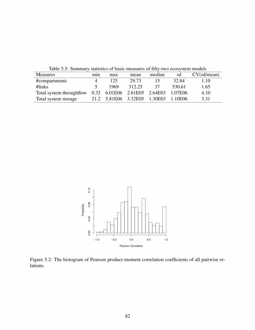
Table 5.5: Summary statistics of basic measures of fifty-two ecosystem modelsMeasures min max mean median sd CV(sd/mean)#compartments 4 125 29.73 15 32.84 1.10#links 5 1969 312.25 37 530.61 1.65Total system throughflow 0.32 6.01E06 2.61E05 2.64E03 1.07E06 4.10Total system storage 21.2 5.81E06 3.32E05 1.30E03 1.10E06 3.31

Pearson Correlation

Pro

ba

bili

ty

−1.0 −0.5 0.0 0.5 1.0

0.0

00

.04

0.0

80

.12

Figure 5.2: The histogram of Pearson product-moment correlation coefficients of all pairwise re-lations.

82

5.3.2 Cluster analysis

Cluster analysis is a widely used method to partition a set of objects into two or more clusters based

on their similarities (Johnson and Wichern, 2002). The set of objects in this work are the forty

system-wide measures. The measures in the same cluster are more similar to each other than those

in different clusters. The similarity of measures is assessed by a distance metric defined between

the measures. Smaller distance represents higher similarity. This distance metric can be defined in

multiple ways, such as Euclidean distance, 1 - correlation, and 1 - abs(correlation). The notation

“abs(x)” represents the absolute value of x. In this work, we adopt 1-abs(Pearson correlation)

as the distance between any two measures, because smaller values of 1-abs(Pearson correlation)

indicate higher (either positive or negative) correlation or similarity between two measures.

After selecting the distance, various methods are available to develop clusters, such as single link-

age, complete linkage, average linkage, Ward’s method, and centroid method. There is no defini-

tive answer as to which method is the best choice. In this work, we will use the simplest and most

efficient method, single linkage, also known as the nearest neighbor technique. This method is

sensitive to outliers, but suffers from the chaining effects (Johnson and Wichern, 2002). The defin-

ing feature of this method is that the distance between clusters is specified as the distance between

the closest pair of measures in these two clusters. Here is the procedure:

1. Start with forty clusters where each measure is one cluster. The distance between any two

measures is 1-abs(Pearson correlation).

2. Place the two measures with the smallest distance into a single cluster.

3. Define the distance between two clusters as the distance between the closest pair of measures

from these two clusters.

4. Merge the two nearest clusters into a single cluster.

5. Repeat steps 3 and 4 until all forty measures are within one cluster.

83

Figure 5.3 shows the cluster dendrogram using 1-abs(Pearson correlation) as the distance metric.

The y-axis represents the distance between clusters (or between measures if there is only one

measure in each cluster). Letter r will be used to represent the Pearson correlation coefficient of

two measures.

5.3.3 Observations and analyses by clusters

In the cluster dendrogram (Figure 5.3), the branches of all measures are colored in red, black or

blue to denote structure-based, flow-based or storage-based measures, respectively. A clustering

of the measures is obtained by cutting the dendrogram at the desired level, then each connected

component forms a cluster. Cutting the dendrogram at different distances gives different sets of

clusters. As we are interested in highly correlated measures, we would like to select a rather small

distance 0.1. At a distance of 0.1, we draw rectangles around all the clusters with more than

one measure. These clusters represent all the measures with a distance of less than or equal to

0.1. Twenty-eight out of forty measures are included in these clusters, shown in Figure 5.3. We

observe that each of these clusters contains only one type of measure: either all structure-based,

or all flow-based, or all storage-based. There isn’t any cross correlation between measures from

different groups (structure-based, flow-based and storage-based). Therefore, in Figure 5.3, we also

color the rectangles that define the clusters in red, black or blue to denote the clusters of structure-

based, flow-based or storage-based measures, respectively. Next, we discuss these three sets of

clusters one by one.

(1) Clusters of structure-based measures (red rectangles)

There are two clusters that contain structure-based measures. The larger one has four measures:

link density, degree diversity, #compartments (network size) and #links. The high correlations

84

System RTTotal system storage

Mean storage #big SCC

Connectance over all pathPercent nodes in big SCC

Mean throughflowInternal overheadTotal internal flow

Total system throughflowTotal system throughput

Internal ascendencyCapacity

OverheadInternal capacity

Total boundary inputAscendency

Biomass diversityConnectance over direct path

#SCCSynergism

Throughflow diversityLink density

Degree diversity #compartments

#linksInternal Ascendency/Capacity

Internal Overhead/CapacityMutualism

RobustnessAscendency/Capacity

Overhead/CapacityAverage path length

I/DHomogenization

SCIAmplification

IEIFCI

Amplification percentage

0.0 0.1 0.2 0.3 0.4 0.5 0.6

Distance = 1 − A

bs(Pearson C

orrelation)

Distance

Figure 5.3: Cluster dendrogram of system-wide measures based on 1-abs(Pearson correlation). Ata distance of 0.1, all clusters with more than one measure are bordered with rectangles.

85

0 20 40 60 80 100 120

510

15

#compartments

Lin

k d

ensity

(a)

0 20 40 60 80 100 120

0.1

0.2

0.3

0.4

#compartments

Connecta

nce (

ove

r direct path

)

(b)

Figure 5.4: (a) Link density vs #compartments; (b) Connectance vs #compartments.

among these four measures indicate that with increase of network size, link density, degree diver-

sity and #links increase as well. It is obvious that degree diversity and #links increase with network

size. We focus below on discussing the counterintuitive increase of link density with network size.

Link density and another related measure, connectance, have been studied in multiple works. As

we have referred in the introduction, there is a debate as to how they change with network size.

For models in Table 5.4, Figure 5.4 shows that the link density (m/n) increases with network size,

while the connectance (m/n2) decreases slightly with network size. This indicates the total number

of links (m) increases faster than the network size n, but slower than n2.

The increase of link density is probably due to two important steps in developing network mod-

els. The first step is to identify the system of interest and place a boundary around it. Because

of this boundary, the connections between compartments in the system and compartments outside

are either ignored, or simply counted as boundary input or output. This reduces the number of

non-boundary links that actually connect to a compartment. The smaller the network, the more

the reduction. If network size increases by expanding the network boundary, some links that were

86

previously ignored will be counted as between-compartment connections. This is one reason that

causes the increase of link density with network size. The second one relates to grouping of cate-

gories. All network models are simplifications of the real ecosystems. Once the system boundary

is set, it is necessary to compartmentalize the system. Different compartments may be grouped as

one big compartment. The connections among the species within the same compartment are not

counted as between-compartment links. The more aggregated the model, the larger the number of

links ignored. On the other hand, decreasing the degree of aggregation during modeling, the num-

ber of links increases, and so does the link density. Both reasons may contribute to the increase of

link density with network size. However, it is difficult to assess in general how significant these

effects are.

One interesting observation about this four-measure cluster is that only the structure-based mea-

sures are significantly affected by network size. As we have referred in the introduction, Fath

(2004) shows how four system-wide measures (amplification, homogenization, synergism and in-

direct effects) change with network size. This analysis shows the four flow-based measures, am-

plification (r = -0.24), homogenization (r = -0.31), synergism (r = -0.44) and indirect effects (r =

-0.34), have weak relationships with network size.

The second cluster containing structure-based measures includes connectance over all paths and

percent nodes in big strongly connected components (SCC). SCC is a subset of the compartments

such that (i) every compartment in the subset has a path to every other and (ii) the subset is not part

of some larger set with the property that every compartment can reach every other. An SCC with

more than one compartment is defined as a big SCC. Connectance over all paths is the proportion

of pairwise compartments that are connected through either direct or indirect paths. Percent nodes

in big SCC is the proportion of compartments that are in big SCCs. Connectance over all paths and

percent nodes in big SCC, respectively, represent how well compartments are connected through

direct or indirect links, and how compartments are mutually reachable. Both measures quantify

the strength of the connections among all compartments.

(2) Clusters of flow-based measures (black rectangles)

87

In Figure 5.3, there are totally five clusters of flow-based measures. Measures in two clusters (as-

cendency/capacity and overhead/capacity, internal ascendency/capacity and internal overhead/capacity)

have perfect negative linear correlations (r = -1), which are due to their algebraic relations (ascen-

dency/capacity + overhead/capacity = 1 and internal ascendency/capacity + internal overhead/capacity

= 1). We disregard them and focus on the other three clusters.

The largest cluster with black rectangle contains eleven measures, including mean throughflow,

internal overhead, total internal flow, total system throughflow, total system throughput, internal

ascendency, capacity, overhead, internal capacity, total boundary input, and ascendency. The def-

initions of these measures are included in the appendix. We would like to point out the subtle

difference between total system throughflow and total system throughput. The former is defined as

the sum of throughflows (∑Ti) and the latter is defined as either ∑Ti+∑zi or ∑Ti+∑yi. Five mea-

sures (mean throughflow, total internal flow, total system throughflow, total system throughput, and

total boundary input) in this cluster are the sum or the mean of some flows in the system, therefore

the high correlations among them are easily understandable. For example, systems receiving high

input (total boundary input) tend to have high total system throughflow as well.

Interestingly, capacity, ascendency, overhead and their internal versions are also classified into this

cluster. The scatter plot in Figure 5.5(a) clearly shows capacity, ascendency, and overhead increase

linearly with respect to total system throughput. Similarly, there are strong positive linear relations

between internal versions of capacity, ascendency and overhead with respect to total internal flow,

the sum of all elements in flow matrix F (Figure 5.5(b)). The formulations of capacity, ascendency

and overhead are

Capacity = −∑i, j

GFi jlog(

GFi j

GF..

)Ascendency = ∑

i, jGFi jlog

(GFi jGF..GFi.GF. j

)(5.1)

Overhead = −∑i, j

GFi jlog

(GF2

i j

GFi.GF. j

)

88

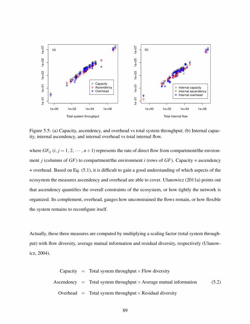
1e+00 1e+02 1e+04 1e+06

1e−

01

1e+

01

1e+

03

1e+

05

1e+

07

Total system throughput

Capacity

Ascendency

Overhead

(a)

1e+00 1e+02 1e+04 1e+06

1e−

01

1e+

01

1e+

03

1e+

05

1e+

07

Total internal flow

Internal capacity

Internal ascendency

Internal overhead

(b)

Figure 5.5: (a) Capacity, ascendency, and overhead vs total system throughput; (b) Internal capac-ity, internal ascendency, and internal overhead vs total internal flow.

where GFi j (i, j = 1, 2, · · · , n+1) represents the rate of direct flow from compartment/the environ-

ment j (columns of GF) to compartment/the environment i (rows of GF). Capacity = ascendency

+ overhead. Based on Eq. (5.1), it is difficult to gain a good understanding of which aspects of the

ecosystem the measures ascendency and overhead are able to cover. Ulanowicz (2011a) points out

that ascendency quantifies the overall constraints of the ecosystem, or how tightly the network is

organized. Its complement, overhead, gauges how unconstrained the flows remain, or how flexible

the system remains to reconfigure itself.

Actually, these three measures are computed by multiplying a scaling factor (total system through-

put) with flow diversity, average mutual information and residual diversity, respectively (Ulanow-

icz, 2004).

Capacity = Total system throughput×Flow diversity

Ascendency = Total system throughput×Average mutual information (5.2)

Overhead = Total system throughput×Residual diversity

89

Table 5.6: Summary statistics of total system throughput, capacity, ascendency, overhead, flowdiversity, average mutual information, and residual diversity.

Measures min max mean median sd CV(sd/mean)Total system throughput 0.42 7.50E06 3.24E05 3.71E03 1.32E06 4.08Capacity 1.63 3.98E07 1.57E06 1.68E04 6.65E06 4.24Ascendency 0.65 1.55E07 6.16E05 5.96E03 2.60E06 4.23Overhead 0.98 2.43E07 9.51E05 1.12E04 4.05E06 4.26Flow diversity 1.16 5.36 3.81 3.94 1.01 0.27Average mutual information 0.94 2.09 1.52 1.43 0.32 0.21Residual diversity 0.11 3.88 2.29 2.34 0.97 0.42

The formulas of flow diversity, average mutual information and residual diversity are shown in Eqs.

(6.7), (6.8) and (6.9), where flow diversity is the sum of average mutual information and residual

diversity. Table 5.6 shows summary statistics (minimum, maximum, mean, median, standard de-

viation and coefficient of variation) of seven measures in Eq. (5.2). Coefficient of variation (CV),

calculated as the ratio of the standard deviation to the mean, is a normalized measure of dispersion.

It is used to compare the scatter of variables expressed in different units or widely different means.

We observe that CVs of flow diversity, average mutual information and residual diversity are much

smaller than those of capacity, ascendency and overhead. In contrast, total system throughput and

three scaled measures (capacity, ascendency and overhead) have similar CVs. This indicates the

changes of capacity, ascendency and overhead are dominated by the scaling factor total system

throughput. The small changes in flow diversity, average mutual information and residual diversity

are almost negligible.

Due to their high correlations with total system throughput, ascendency and overhead may not be

as useful in quantifying the network organization as Ulanowicz (2011a) indicates. For example,

different networks with the same total system throughput may have very different (either constraint

or flexible) network organizations. However, due to the same value of total system throughput, the

two measures ascendency and overhead are also similar for these networks. In this case, two

measures ascendancy and overhead values somewhat fail to quantify the different organizations

90

inherent in these networks. Considering their complex computations, capacity, ascendency and

overhead do not provide much further useful information than total system throughput, which has

a rather simple definition.

Internal capacity, internal ascendency and internal overhead, respectively, are part of capacity,

ascendency and overhead that are contributed by inter-compartmental flows. The difference is that

the former three do not take into account environmental input and output, while the latter three do.

As the system with higher total system throughput tends to have higher inter-compartmental flows,

it makes sense that capacity, ascendency and overhead are not that different from their internal

versions.

Because of their strong correlations with total system throughput, capacity, ascendency and over-

head may not be useful in quantifying network organization, even though they are conceptually,

and therefore qualitatively, valuable. Also, the ratios of ascendency to capacity and overhead

to capacity are very informative. According to Ulanowicz (2009, 2011a), ascendency/capacity

(equivalent to average mutual information/flow diversity) represents the degree of organization and

overhead/capacity (equivalent to residual diversity/flow diversity) represents the degree of flexibil-

ity. Whether a system has very high ascendency/capacity and low overhead/capacity, or vice-versa,

makes a significant difference. If ascendency/capacity is too high, the system will be very efficient,

but very vulnerable to perturbation. If ascendency/capacity is too low, it lacks sufficient cohesion

to hold together. Sustainable ecosystems exhibit a narrow range of ascendency/capacity. The back

and forth between ascendency/capacity and overhead/capacity is analogous to the Yin-Yang di-

alectic of Eastern thought (Ulanowicz, 2011b). Our statistical analysis shows that these ratios truly

provide new information, and are not correlated with system throughflow and any other measure.

But further efforts are needed to fully understand why two ratios are as informative about the net-

work organization as they appear to be. As this is not the main focus of this work, we refer the

reader to Ulanowicz (2004, 2009, 2011a).

Ulanowicz (2009) observes that well-articulated networks of trophic flows from a wide variety of

ecosystems cluster around values of ascendency/capacity≈ 40% and overhead/capacity≈ 60%. In

91

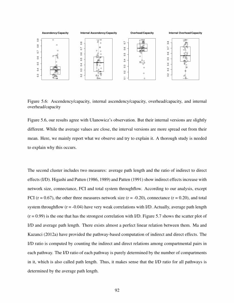
0.3

0.4

0.5

0.6

0.7

0.8

0.9

Ascendency/Capacity

0.2

0.3

0.4

0.5

0.6

0.7

0.8

Internal Ascendency/Capacity

0.1

0.2

0.3

0.4

0.5

0.6

0.7

Overhead/Capacity

0.2

0.3

0.4

0.5

0.6

0.7

0.8

Internal Overhead/Capacity

Figure 5.6: Ascendency/capacity, internal ascendency/capacity, overhead/capacity, and internaloverhead/capacity

Figure 5.6, our results agree with Ulanowicz’s observation. But their internal versions are slightly

different. While the average values are close, the interval versions are more spread out from their

mean. Here, we mainly report what we observe and try to explain it. A thorough study is needed

to explain why this occurs.

The second cluster includes two measures: average path length and the ratio of indirect to direct

effects (I/D). Higashi and Patten (1986, 1989) and Patten (1991) show indirect effects increase with

network size, connectance, FCI and total system throughflow. According to our analysis, except

FCI (r = 0.67), the other three measures network size (r = -0.20), connectance (r = 0.20), and total

system throughflow (r = -0.04) have very weak correlations with I/D. Actually, average path length

(r = 0.99) is the one that has the strongest correlation with I/D. Figure 5.7 shows the scatter plot of

I/D and average path length. There exists almost a perfect linear relation between them. Ma and

Kazanci (2012a) have provided the pathway-based computation of indirect and direct effects. The

I/D ratio is computed by counting the indirect and direct relations among compartmental pairs in

each pathway. The I/D ratio of each pathway is purely determined by the number of compartments

in it, which is also called path length. Thus, it makes sense that the I/D ratio for all pathways is

determined by the average path length.

92

1 2 5 10 20 50 100 200

0.1

0.5

5.0

50.0

Average path length

I/D

Figure 5.7: I/D vs average path length

A further study shows average path length (r = -0.19) also doesn’t change much with network

size. This is mainly because the number of trophic levels in most durable natural ecosystems is

about four (Matsuno and Ono, 1996). Without considering cycling, the maximum path length for

ecosystems of any size should be around four as well. The average path length should be even

smaller. Thus, the increase of path length is not due to increasing network size. Instead, it is due

to the occurrence of cycling, which is represented as the repeated compartments in long pathways.

The third cluster is FCI and amplification percentage. FCI, the proportion of cycled total system

throughflow, is computed using diagonal elements Nii of throughflow analysis matrix. Amplifi-

cation is the number of off-diagonal elements Ni j(i 6= j) that are larger than 1. To enable the

comparison of amplification across networks of different size, we define a normalized version of

amplification, called amplification percentage. It is computed as amplification/(n(n-1)), where n is

network size. The high correlation between FCI and amplification indicates that the off-diagonal

elements of the throughflow matrix N tend to be larger than 1 as the diagonal elements get larger.

Fath (2004) has used large-scale cyber-ecosystems to show that amplification only occurs spar-

93

ingly in smaller networks. Our analysis shows the occurrence of amplification is more dependent

on the strength of cycling (r = 0.92), and less on network size (r = -0.37). The reason why Fath

(2004) does not observe high amplification in his cyber-ecosystems is probably due to the fact that

these networks have low cycling index (FCI ∈(0.14, 0.25)). Large networks with strong cycling

also have high amplification.

(3) Clusters of storage-based measures (blue rectangles)

The only storage-based cluster contains three measures: system residence time (system RT), total

system storage and mean storage. Mean storage is the average storage of all compartments in the

system. Total system storage is the sum of storage at all compartments in the system. A very strong

linear correlation (r = 0.99) exists between these two storage measures. System RT is defined as

the average total time that flow material stays in the system. Its high correlation with total system

storage (r = 0.93) indicates the flow material tends to stay longer when the system storage increases.

These three storage-based measures (total system storage, mean storage and system RT) parallel

another three flow-based measures (total system throughflow, mean throughflow and average path

length). The key difference is that the former three take into account the residence time in each

compartment, while the latter three do not. For example, average path length only counts the num-

ber of compartments the flow material passes through before exiting the system, while system RT

is defined as the sum of the residence time in these compartments. However, total system storage (r

= -0.05) is almost uncorrelated with total system throughflow. Mean storage and mean throughflow

are also uncorrelated (r = -0.06). There is also very weak correlation between system RT and av-

erage path length (r = -0.04). In addition to these three measures (total system throughflow, mean

throughflow and average path length), other flow-based measures are also not correlated with three

storage-based measures. We often take for granted that a system with high storage tends to have

high flow values as well. The weak correlations indicate storage introduces new and independent

information and it is very difficult to statistically derive it from the flow values, and vice versa.

Storage plays an important role in generating network properties, and therefore should not be ig-

nored in developing system measures. However, very few existing measures utilize the storage

94

values. The development of more novel storage-based measures may help to capture new holistic

properties of the ecological networks.

5.3.4 Other observations and analyses

Among these forty measures, some measures (e.g. two connectance measures, two cycling indices,

and three diversity measures) are defined similarly, or using the same concept. Next, we compare

how they are different.

The first set is two measures of connectance. Connectance quantifies the proportion of realized

links between compartments. Some compartments, that are not linked directly, may be connected

through indirect paths that are transmitted by others. So, we compute two connectance measures:

one is realized by direct links and the other is realized by both direct and indirect links. Figure

5.8 shows the boxplots of these two connectance measures. We can see that connectance over all

paths (≈ 0.80) is much higher than that due to direct paths only (≈ 0.23). The difference of two

is the connectance over indirect paths only (≈ 0.56). This indicates most of compartments are

connected only through indirect paths. Even these directly connected compartments may also be

connected through indirect paths. Higashi and Patten (1989) and Salas and Borrett (2011) show

that indirect effects in ecological networks are significantly dominant. Our result, from a purely

network structure point of view (based on adjacency matrix only), supports the dominance of

indirect effects in the ecosystem.

The second set is the three diversity measures: degree diversity, biomass diversity and throughflow

diversity. Shannon index (Shannon, 2001) is a popular diversity index. MacArthur (1955) applied

Shannon’s information measure to the storage values of all compartments in an ecosystem network,

called biomass diversity. It is affected by both the number of compartments and the evenness of

95

0.1

0.2

0.3

0.4

Connectance over direct path

0.4

0.6

0.8

1.0

Connectance over all path

Figure 5.8: Connectance over direct paths vs connectance over all paths

storage. A greater number of species and a more even distribution of species abundance contribute

to an increase in Shannon’s diversity. We also define similar diversity measures for the degree (the

number of links) and throughflow values of all compartments. In the cluster dendrogram (Figure

5.3), these three diversity measures are separated in different clusters. Figure 5.9 shows how the

three diversity measures change with respect to network size. As the number of compartments

increases, degree diversity exhibits a monotonic increase, throughflow diversity increases slightly,

but biomass diversity does not show any trend. For the same network, the ranking of these three

diversity values tends to be: degree diversity > throughflow diversity > biomass diversity, although

this is not always expressed for throughflow and biomass. This ordering indicates degrees of all

compartments are more evenly distributed than throughflows, and throughflows are more evenly

distributed than storage values. That is, all compartments in a network tend to have much more

similar degrees than throughflows and biomass values.

The third pair is the two cycling indices: Finn’s cycling index (FCI) and storage-based cycling

index (SCI). FCI and SCI compute the proportion of cycled total system throughflow and total

system storage, respectively. There is a high correlation (0.82) between two cycling indices, but

for any given network, these two cycling indices can be very different. More detailed discussion

and comparison of these two cycling indices are available in Ma and Kazanci (in press 2014).

96

20 40 60 80 100 120

02

46

8

#compartments

Degree diversity

Throughflow diversity

Biomass diversity

Figure 5.9: Degree diversity, throughflow diversity and biomass diversity vs the number of com-partments

5.4 Conclusion and discussion

The results of this chapter can be summarized as below:

• There is no significant cross correlation between structure-based, flow-based and storage-

based measures.

• Link density (m/n) increases with network size n, while the connectance (m/n2) decreases

slightly with network size.

97

• Capacity, ascendency, and overhead are highly correlated with total system throughput. The

ratios of these measures (ascendency/capacity and overhead/capacity) contain more signifi-

cant, or perhaps independent information than themselves.

• The occurrence of network amplification depends more on the strength of cycling (r = 0.92)

than the network size (r = -0.37).

• The ratio of indirect to direct effects (I/D) is affected more by average path length than

network size.

• Most compartments are linked through indirect connections. This result, from a network

structure point of view, supports the dominance of indirect effects in the ecosystem.

• The evenness of degree, throughflow and storage have the following order: degree > through-

flow > storage. That is, all compartments in a network tend to have much more similar

degrees than throughflows and biomass values.

This work enables a better understanding of the relationship among various measures. Some mea-

sures have stronger correlation than expected, such as the three measures (ascendency, overhead

and capacity) and total system throughput, or I/D and average path length. Some measures may

not have strong correlations as previously reported, such as the relation between indirect effects

with network size, or connectance and total system throughflow.

In practical applications, when researchers have a particular purpose such as to evaluate the sys-

tem cycling, the corresponding measures (e.g. FCI and SCI) can be selected. However, without

such a particular purpose, the selection of measures is not straightforward. System-wide mea-

sures are often selected either based on historical practices or many system-wide measures are

used simultaneously to assess the essential differences between similar networks. As the number

of measures increases, it becomes unnecessary and impractical to apply all available measures.

Some measures, although defined in different ways, behave very similarly, such as I/D and average

98

path length, ascendency and total system throughput. Inclusion of all strongly correlated mea-

sures provides litter extra useful information than using only one representative measure from that

group. And sometimes, when comparing different networks using system-wide measures, what

may be perceived as a similarity between networks may be entirely due to the relationships among

measures. For example, two networks with the same total system throughput may have very differ-

ent network organizations. Without knowing the high correlation of ascendency and total system

throughput, ascendency may be selected to assess the organizations inherent in two networks. In

fact, ascendency, dominated by total system throughput, somewhat fails to indicate the difference

of organizations. Instead, the normalized version ascendency/capacity can serve as a better index

than ascendency. Thus, selection of measures becomes crucial for an informed application of eco-

logical network analysis. A “good” set of measures would include fewer key measures that provide

the most available information. This work provides a comprehensive comparison of all measures,

and can help to select a set of measures to assess ecosystems from difference perspectives.

99

Chapter 6

Conclusions and future work

In this chapter, I briefly summarize the contributions of this dissertation and discuss directions for

future work.

6.1 The contribution of this work

Conventional methods used for Ecological Network Analysis (ENA) are mainly Eulerian ap-

proaches. NPT, through simulating the movements of particles, provides a Lagrangian point of

view of a compartmental model. Prior to this dissertation, NPT had been applied to study FCI

(Kazanci et al., 2009), throughflow analysis (Matamba et al., 2009), and storage analysis (Kazanci

and Ma, 2012). The pathway-based computations of these three measures match their algebraic

formulas. The pathway-based method not only provides a simpler and more intuitive interpretation

for existing system-wide measures, but also helps develop new interesting and useful measures. In

this dissertation, utilizing the pathway-based method, we are able to (1) discover the inaccuracy

of two existing formulations of I/D ratio and provide revision, (2) propose a new storage-based

cycling index (SCI) that is more informative than FCI, (3) develop a pure indirect effects index

that does not depend on cycling, and (4) illustrate the subtle difference between FCI and a com-

100

prehensive cycling index (CCI). Although it has many advantages, NPT does not always succeed

in computing all measures. In Appendix A, we describe our efforts to compute the U matrix us-

ing a pathway-based method, and demonstrate why this method cannot be implemented for utility

analysis.

Potential contribution to other areas

The development of ENA theory and the defining of various measures benefited from the method-

ologies and tools in other areas, such as input-output theory in economics, and information theory.

ENA was originally an extended application of economic input-output analysis to ecology (Leon-

tief, 1966; Hannon, 1973). Several measures (e.g. FCI, I/D, amplification and homogenization)

are defined based on the Leontief structure matrix, which is usually called throughflow analysis

matrix (N) in ENA. Ascendancy and several related measures (Ulanowicz, 1986b) are based on

information theory (Rutledge et al., 1976). Three diversity measures (degree diversity, through-

flow diversity and biomass diversity) are proposed by applying Shannon’s information measure to

degree, throughflow and biomass of all compartments in ecological networks (MacArthur, 1955).

Similarly, recent developments occurring in systems ecology, such as new findings in this disser-

tation, should not be limited to ecological networks. Several new measures proposed in this work,

especially their pathway-based computations, can be potentially applied to any network in which

the flow material being traced is conservative, such as energy, matter, organisms, persons, cells,

paper, iron, etc. Section 3.6 demonstrates the applications of SCI in computing reinfection rate of

infectious diseases in epidemiology (Gomes et al., 2004), and the recycling of material in industrial

systems (Bailey et al., 2008). Similar to SCI, other ENA measures also have potential applications

to network analysis in other areas.

101

6.2 Future work

Future work will continue to develop and search for novel ecological network measures. In addi-

tion, we would like to pursue the application of ENA measures to study realistic ecosystem models,

which often involve dynamic changes.

6.2.1 Development of new ENA measures

The system-wide measures quantify how the ecosystem is performing as a whole. There are also a

set of compartmental measures (e.g. degree, closeness and betweenness) that quantify the impor-

tance of single compartments. We would like to discuss separately future work on the development

of these two types of measures.

(1) Development of system-wide measures

During the study of this dissertation, I feel novel measures are needed to evaluate the ecological

networks as wholes. The development of system-wide measures can focus on the following two

directions: one is to develop more storage-based measures; the other one is to introduce useful

measures from other areas.

While searching the literature for various measures, I realized the majority of system-wide mea-

sures are flow-based. Very few measures utilize the storage values. In addition to flow, storage

plays an important role in generating network properties, and therefore should not be ignored in

developing system measures. In this dissertation, we proposed a storage-based cycling index (SCI),

which parallels the existing flow-based cycling index FCI. Figure 6.1 compares FCI and SCI for

16 seasonal nitrogen flow models for the Neuse River estuary, North Carolina, USA (Christian and

Thomas, 2003). One important characteristic of good indicators is sensitivity to change (Riley,

2000). For these 16 models, SCI is more sensitive to seasonal changes occurring in the systems

than FCI. In addition, SCI is more informative about the system cycling than FCI because it utilizes

flow values used for computing FCI and takes into account residence time as well. Thus, SCI is

102

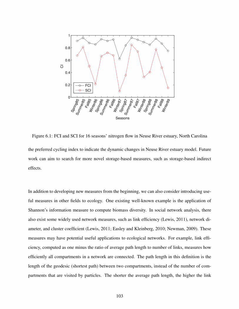
0

0.2

0.4

0.6

0.8

1

Seasons

CI

Spring85

Sum

mer8

5Fall8

5W

inte

r86

Spring86

Sum

mer8

6Fall8

6W

inte

r87

Spring87

Sum

mer8

7Fall8

7W

inte

r88

Spring88

Sum

mer8

8Fall8

8W

inte

r89

FCI

SCI

Figure 6.1: FCI and SCI for 16 seasons’ nitrogen flow in Neuse River estuary, North Carolina

the preferred cycling index to indicate the dynamic changes in Neuse River estuary model. Future

work can aim to search for more novel storage-based measures, such as storage-based indirect

effects.

In addition to developing new measures from the beginning, we can also consider introducing use-

ful measures in other fields to ecology. One existing well-known example is the application of

Shannon’s information measure to compute biomass diversity. In social network analysis, there

also exist some widely used network measures, such as link efficiency (Lewis, 2011), network di-

ameter, and cluster coefficient (Lewis, 2011; Easley and Kleinberg, 2010; Newman, 2009). These

measures may have potential useful applications to ecological networks. For example, link effi-

ciency, computed as one minus the ratio of average path length to number of links, measures how

efficiently all compartments in a network are connected. The path length in this definition is the

length of the geodesic (shortest path) between two compartments, instead of the number of com-

partments that are visited by particles. The shorter the average path length, the higher the link

103

efficiency. In ENA, a flow-based measure, ascendency/capacity, is a reported indicator of system

efficiency. It would be interesting to know how link efficiency and ascendency/capacity differ in

quantifying system efficiency. Another measure, network diameter, the largest geodesic length, is

representative of linear size of a network. This could possibly serve as another useful measure of

network size, in addition to the number of compartments.

One significant difference between ecological and social networks is that the former are directed

while the latter are undirected. The computation of link efficiency, network diameter and cluster

coefficient requires a path matrix (P) that stores the length of geodesic (the shortest path) between

all node pairs (Lewis, 2011). All nodes of an undirected network are mutually reachable through

direct or indirect paths. However, for directed networks, the existence of a path from any com-

partment to all others is unlikely. For example, if a directed path from A to B does not exist,

the length of shortest path from A to B (P(B, A)) is unavailable. Those measures that depend on

path matrix (P) cannot be computed. Therefore, a direct application of social network measures

to ecosystems may not be feasible. Further efforts are necessary to explore this problem. Perhaps

it would be possible to develop some native ENA measures, which have similar interpretations to

social network measures.

(2) Development of compartmental measures

One important application of compartmental measures is to find the key node in a network. For

ecosystems, these can be used to identify key (or keystone) species. A variety of centrality mea-

sures (e.g., degree, closeness and betweenness) have been defined for social networks that are

unweighted and undirected. We realize such measures are not well suited for ecosystems because

they (i) only consider direct links (local connections); or (ii) only apply to networks where all the

nodes are mutually reachable; or (iii) do not take into account the flow weights.

Several works already have aimed to define centrality measures for ecosystems. Borrett (2013)

has proposed throughflow centrality, where throughflow is the total amount of flows from one

compartment to others. It is actually a flow-weighted degree centrality which sums up the flow

104

rates for links exiting (or entering) a node. Although its computation and interpretation are simple,

its disadvantage is it doesn’t take into account the indirect flows. Jordán et al. (1999, 2006) have

proposed bottom-up and top-down keystone indices for food webs. However, these two indices

also do not consider the flow values in the network. Also, they are not applicable to networks with

cycled flows.

Due to these and other limitations of existing measures, the aim of our future work will be to search

for better centrality measures that work well for ecological networks.

6.2.2 Applications of pathway-based ENA

Ecosystems are not static, but subject to natural environmental variations or human impacts. For

example, human activities have led to the degradation of various ecosystems, which is manifested

in a reduction of richness of species. Pathway-based computation extends the applicability of ENA

to dynamic ecosystem models. Kazanci (2011) use a conceptual three-compartment model to show

the pathway-based computation of storage analysis matrix (S) for dynamic models. Future work

will focus on applying pathway-based ENA to study dynamic ecosystem models and investigate

how ecosystems respond to these changes as a whole.

The application of ENA relies in the first instance on the compartmental models formulated to

describe ecosystems. The accuracy of the model determines the quality of analysis. However,

it is difficult and time-consuming to collect the data needed to construct compartmental models,

whose data requirements are substantial. Future work will rely on close collaboration with field

ecologists.

105

Bibliography

Allesina, S., Ulanowicz, R. E., 2004. Cycling in ecological networks: Finn’s index revisited. Com-

putational Biology and Chemistry 28 (3), 227–233.

Almunia, J., Basterretxea, G., Aistegui, J., Ulanowicz, R., 1999. Benthic-pelagic switching in a

coastal subtropical lagoon. Estuarine, Coastal and Shelf Science 49 (3), 363–384.

Bailey, R., Bras, B., Allen, J. K., 2008. Measuring material cycling in industrial systems. Re-

sources, Conservation and Recycling 52 (4), 643–652.

Baird, D., Christian, R., Peterson, C., Johnson, G., 2004. Consequences of hypoxia on estuarine

ecosystem function: energy diversion from consumers to microbes. Ecological Applications

14 (3), 805–822.

Baird, D., Luczkovich, J., Christian, R. R., 1998. Assessment of spatial and temporal variability in

ecosystem attributes of the st marks national wildlife refuge, apalachee bay, florida. Estuarine,

Coastal and Shelf Science 47 (3), 329–349.

Baird, D., McGlade, J., Ulanowicz, R., Baird, D., McGlade, J., Ulanowicz, R., 1991. The com-

parative ecology of six marine ecosystems. Philosophical Transactions of the Royal Society of

London. Series B: Biological Sciences 333 (1266), 15–29.

Baird, D., Milne, H., 1981. Energy flow in the ythan estuary, aberdeenshire, scotland. Estuarine,

Coastal and Shelf Science 13 (4), 455–472.

106

Baird, D., Ulanowicz., R., 1989. The seasonal dynamics of the chesapeake bay ecosystem. Ecol.

Monogr., 59: 329–364.

Baird, D., Ulanowicz, R., 1993. Comparative study on the trophic structure, cycling and ecosystem

properties oi iour tidal. Mar. Ecol. Prog. Ser 99, 221–237.

Bondavalli, C., Ulanowicz, R. E., 1999. Unexpected effects of predators upon their prey: the case

of the american alligator. Ecosystems 2 (1), 49–63.

Borrett, S., Freeze, M., 2010. Reconnecting environs to their environment. Ecological Modelling.

Borrett, S., Freeze, M., Salas, A., 2011. Equivalence of the realized input and output oriented

indirect effects metrics in ecological network analysis. Ecological Modelling 222, 2142–2148.

Borrett, S., Lau, M., 2012. Vignette: enar.

Borrett, S., Whipple, S., Patten, B., 2010. Rapid development of indirect effects in ecological

networks. Oikos 119 (7), 1136–1148.

Borrett, S. R., 2013. Throughflow centrality is a global indicator of the functional importance of

species in ecosystems. Ecological Indicators 32, 182–196.

Brylinsky, M., 1972. Steady-state sensitivity analysis of energy flow in a marine ecosystem. Sys-

tems analysis and simulation in ecology 2, 81–101.

Buzhdygan, O. Y., Patteny, B. C., Rudenko, S. S., 2012. Trophic network analysis: Comparison of

system-wide properties. Models of the Ecological Hierarchy: From Molecules to the Ecosphere

25, 181.

Chen, S., Chen, B., 2011. Defining indirect uncertainty in system-based risk management. Ecolog-

ical Informatics.

107

Christian, R. R., Baird, D., Luczkovich, J., Johnson, J. C., Scharler, U. M., Ulanowicz, R. E., 2005.

Role of network analysis in comparative ecosystem ecology of estuaries. Aquatic Food Webs.

Oxford University Press, Oxford, 25–40.

Christian, R. R., Thomas, C. R., 2000. Neuse river estuary modeling and monitoring project stage

1: Network analysis for evaluating the consequences of nitrogen loading.

Christian, R. R., Thomas, C. R., 2003. Network analysis of nitrogen inputs and cycling in the neuse

river estuary, north carolina, usa. Estuaries 26 (3), 815–828.

Chrystal, R. A., Scharler, U. M., 2014. Network analysis indices reflect extreme hydrodynamic

conditions in a shallow estuarine lake (lake st lucia), south africa. Ecological Indicators 38,

130–140.

Cohen, J. E., Briand, F., 1984. Trophic links of community food webs. Proceedings of the National

Academy of Sciences 81 (13), 4105–4109.

Dame, R. F., Patten, B. C., 1981. Analysis of energy flows in an intertidal oyster reef. Marine

Ecology Progress Series 5 (2), 115–124.

DeAngelis, D., 1980. Energy flow, nutrient cycling, and ecosystem resilience. Ecology, 764–771.

DeAngelis, D., Mulholland, P., Palumbo, A., Steinman, A., Huston, M., Elwood, J., 1989. Nutrient

dynamics and food-web stability. Annual Review of Ecology and Systematics 20, 71–95.

Easley, D., Kleinberg, J., 2010. Networks, crowds, and markets. Vol. 8. Cambridge Univ Press.

Edmisten, J., 1970. Preliminary studies of the nitrogen budget of a tropical rain forest. In: Odum,

H., Pigeon, R. (Eds.), A Tropical Rain Forest. TID-24270. USAEC Technical Information Cen-

ter, Oak Ridge, Tennessee., pp. 211–215.

Fath, B., 2004. Network analysis applied to large-scale cyber-ecosystems. Ecological Modelling

171 (4), 329–337.

108

Fath, B. D., Borrett, S. R., 2006. A MATLAB® function for network environ analysis. Environ-

mental Modelling and Software 21 (3), 375–405.

Fath, B. D., Halnes, G., 2007. Cyclic energy pathways in ecological food webs. Ecological Mod-

elling 208 (1), 17–24.

Fath, B. D., Patten, B. C., 1999a. Quantifying resource homogenization using network flow analy-

sis. Ecological Modelling 123 (2-3), 193–205.

Fath, B. D., Patten, B. C., 1999b. Review of the foundations of network environ analysis. Ecosys-

tems 2, 167.

Fenchel, T., Blackburn, T. H., et al., 1979. Bacteria and mineral cycling. Academic Press,

Inc.(London) Ltd.

Finn, J., 1977. Flow analysis: A method for tracing flows through ecosystem models. Ph.D. thesis,

University of Georgia.

Finn, J. T., 1976. Measures of ecosystem structure and function derived from analysis of flows.

Journal of Theoretical Biology 56 (2), 363–80.

Finn, J. T., 1978. Cycling index: a general difinition for cycling in compartment models. In: Adri-

ano, D., Brisbin, I. (Eds.), Environmental Chemistry and Cycling Processes, U.S. Dep. Energy

Symp. Vol. 45. National Technical Information Center, Springfield, VA, pp. 148–164.

Finn, J. T., Jun 1980. Flow analysis of models of the hubbard brook ecosystem. Ecology 61 (3),

562–571.

FitzGerald, G. J., 1992. Filial cannibalism in fishes: why do parents eat their offspring? Trends in

Ecology & Evolution 7 (1), 7–10.

Fraser, C., Donnelly, C. A., Cauchemez, S., Hanage, W. P., Van Kerkhove, M. D., Hollingsworth,

T. D., Griffin, J., Baggaley, R. F., Jenkins, H. E., Lyons, E. J., et al., 2009. Pandemic potential of

a strain of influenza a (h1n1): early findings. science 324 (5934), 1557–1561.

109

Freeman, L. C., 1979. Centrality in social networks conceptual clarification. Social networks 1 (3),

215–239.

Gillespie, D. T., 1977. Exact stochastic simulation of coupled chemical reactions. Journal of Phys-

ical Chemistry 81 (25), 2340–2361.

Gomes, M. G. M., White, L. J., Medley, G. F., 2004. Infection, reinfection, and vaccination un-

der suboptimal immune protection: epidemiological perspectives. Journal of theoretical biology

228 (4), 539–549.

Grayston, J. T., Wang, S.-p., Yeh, L.-j., Kuo, C.-c., 1985. Importance of reinfection in the patho-

genesis of trachoma. Review of Infectious Diseases 7 (6), 717–725.

Hannon, B., 1973. The structure of ecosystems. Journal of Theoretical Biology 41 (3), 535–46.

Hatanaka, T., Honda, S., Sasaki, S., Katayama, K., Koizumi, T., 1998. Pharmacokinetic and phar-

macodynamic evaluation for tissue-selective inhibition of cholesterol synthesis by pravastatin.

Journal of Pharmacokinetics and Pharmacodynamics 26 (3), 329–347.

Havens, K., 1992. Scale and structure in natural food webs. Science 257 (5073), 1107–1109.

Hazen, R. M., Hemley, R. J., Mangum, A. J., 2012. Carbon in earth’s interior: Storage, cycling,

and life. Eos, Transactions American Geophysical Union 93 (2), 17–18.

Herendeen, R., 1989. Energy intensity, residence time, exergy, and ascendency in dynamic ecosys-

tems. Ecological Modelling 48 (1), 19–44.

Heymans, J., Baird, D., 2000. A carbon flow model and network analysis of the northern benguela

upwelling system, namibia. Ecological Modelling 126 (1), 9–32.

Higashi, M., Patten, B. C., 1986. Further aspects of the analysis of indirect effects in ecosystems.

Ecological Modelling 31 (1), 69–77.

110

Higashi, M., Patten, B. C., 1989. Dominance of indirect causality in ecosystems. American Natu-

ralist 133 (2), 288.

Jackson, J. B., 2006. When ecological pyramids were upside down. Whales, whaling, and ocean

ecosystems, 27–37.

Johnson, R. A., Wichern, D. W., 2002. Applied multivariate statistical analysis. Vol. 5. Prentice

hall Upper Saddle River, NJ.

Jordan, C., Kline, J., Sasscer, D., 1972. Relative stability of mineral cycles in forest ecosystems.

American Naturalist 106, 237–253.

Jordán, F., Liu, W.-c., Davis, A. J., 2006. Topological keystone species: measures of positional

importance in food webs. Oikos 112 (3), 535–546.

Jordán, F., Takács-Sánta, A., Molnár, I., 1999. A reliability theoretical quest for keystones. Oikos,

453–462.

Jørgensen, S. E., Burkhard, B., Müller, F., 2013. Twenty volumes of ecological indicators–an

accounting short review. Ecological Indicators 28, 4–9.

Jorgensen, S. E., Xu, F.-L., Costanza, R., 2005. Handbook of ecological indicators for assessment

of ecosystem health. CRC press.

Kazanci, C., 2007. Econet: A new software for ecological modeling, simulation and network

analysis. Ecological Modelling 208 (1), 3–8.

Kazanci, C., 2009. Handbook of Ecological Modelling and Informatics. WIT Press, Ch. Network

calculations II: a user’s manual for EcoNet, pp. 325–350.

Kazanci, C., 2011. Network particle tracking (NPT): An individual based simulation algorithm

compatible with the differential equation representation for network models., in Preparation.

111

Kazanci, C., Ma, Q., 2012. Dynamic storage analysis and residence time distribution for open

compartmental systems, in Preparation.

Kazanci, C., Matamba, L., Tollner, E. W., 2009. Cycling in ecosystems: An individual based

approach. Ecological Modelling (220), 2908–2914.

Krivtsov, V., 2004. Investigations of indirect relationships in ecology and environmental sciences:

a review and the implications for comparative theoretical ecosystem analysis. Ecological mod-

elling 174 (1), 37–54.

Krivtsov, V., 2009. Indirect effects in ecology. Ecosystem Ecology, 81.

Leontief, W., 1951. The structure of American economy, 1919-1929: An empirical application of

equilibrium analysis. Harvard University Press.

Leontief, W., 1966. Input-output economics. Oxford University Press, USA.

Lewis, T. G., 2011. Network science: Theory and applications. John Wiley & Sons.

Link, J., Overholtz, W., O’Reilly, J., Green, J., Dow, D., Palka, D., Legault, C., Vitaliano, J., Guida,

V., Fogarty, M., et al., 2008. The northeast us continental shelf energy modeling and analysis

exercise (emax): ecological network model development and basic ecosystem metrics. Journal

of Marine Systems 74 (1), 453–474.

Lobanova, G., Fath, B., Rovenskaya, E., 2009. Exploring simple structural configurations for op-

timal network mutualism. Communications in Nonlinear Science and Numerical Simulation

14 (4), 1461–1485.

Loreau, M., 1994. Material cycling and the stability of ecosystems. The American Naturalist

143 (3), 508–513.

Ma, Q., Kazanci, C., 2012a. Analysis of indirect effects within ecosystem models using pathway-

based methodology. Ecological Modelling 252, 238–245.

112

Ma, Q., Kazanci, C., 2012b. An individual-based approach for studying system-wide properties of

ecological networks. Models of the Ecological Hierarchy: From Molecules to the Ecosphere 25,

201.

Ma, Q., Kazanci, C., in press 2014. How much of the storage in the ecosystem is due to cycling?

Journal of Theoretical Biology.

MacArthur, R., 1955. Fluctuations of animal populations and a measure of community stability.

ecology 36 (3), 533–536.

Martinez, N. D., 1992. Constant connectance in community food webs. American Naturalist,

1208–1218.

Matamba, L., Kazanci, C., Schramski, J. R., Blessing, M., Alexander, P., Patten, B., 2009.

Throughflow analysis: a stochastic approach. Ecological Modelling 220, 3174–3181.

Matis, J. H., Patten, B. C., 1981. Environ analysis of linear compartmental systems: the static, time

invariant case. Bulletin International Statistics Institute 48, 527–565.

Matsuno, K., Ono, N., 1996. How many trophic levels are there? Journal of theoretical biology

180 (2), 105–109.

Miehls, A., Mason, D., Frank, K., Krause, A., Peacor, S., Taylor, W., 2009a. Invasive species

impacts on ecosystem structure and function: A comparison of oneida lake, new york, usa,

before and after zebra mussel invasion. Ecological Modelling 220 (22), 3194–3209.

Miehls, A., Mason, D., Frank, K., Krause, A., Peacor, S., Taylor, W., 2009b. Invasive species

impacts on ecosystem structure and function: A comparison of the bay of quinte, canada, and

oneida lake, usa, before and after zebra mussel invasion. Ecological Modelling 220 (22), 3182–

3193.

113

Min, Y., Jin, X., Chang, J., Peng, C., Gu, B., Ge, Y., Zhong, Y., 2011. Weak indirect effects inher-

ent to nitrogen biogeochemical cycling within anthropogenic ecosystems: A network environ

analysis. Ecological Modelling 222 (17), 3277–3284.

Monaco, M., Ulanowicz, R., 1997. Comparative ecosystem trophic structure of three us mid-

atlantic estuaries. Marine Ecology Progress Series 161, 239–254.

Newman, M., 2009. Networks: an introduction. Oxford University Press.

Odum, E. P., 1969. The strategy of ecosystem development. Science 164 (3877), 262–270.

Odum, E. P., 1971. Fundamentals of ecology, 574 pp. Philadelphia: Saunders.

Odum, H. T., 1957. Trophic structure and productivity of silver springs, florida. Ecological Mono-

graphs, 55–112.

Patrício, J., Ulanowicz, R., Pardal, M. A., Marques, J. C., 2004. Ascendency as an ecological

indicator: a case study of estuarine pulse eutrophication. Estuarine, Coastal and Shelf Science

60 (1), 23–35.

Patten, B., 1991. Network ecology: indirect determination of the life-environment relationship in

ecosystems. Theoretical Studies of Ecosystems. Cambridge University Press, Cambridge, 288–

351.

Patten, B. C., 1978. Systems approach to the concept of environment. Ohio Journal of Science

78 (4), 206–222.

Patten, B. C., 1985a. Energy cycling in the ecosystem. Ecological modelling 28, 1–71.

Patten, B. C., 1985b. Energy cycling, length of food chains, and direct versus indirect effects in

ecosystems. Can. Bull. Fish. Aqu. Sci. 213, 119–113.

114

Patten, B. C., 1986. Energy cycling, length of food chains, and direct versus indirect effects in

ecosystems. Ecosystem Theory for Biological Oceanography. Can. Bull. Fish. Aquat. Sci 213,

119–138.

Patten, B. C., 1995. Network integration of ecological extremal principles: exergy, emergy, power,

ascendency, and indirect effects. Ecological Modelling 79, 75–84.

Patten, B. C., Higashi, M., Oct 1984. Modified cycling index for ecological applications. Ecologi-

cal Modelling 25, 69–83.

Pregitzer, K. S., Euskirchen, E. S., 2004. Carbon cycling and storage in world forests: biome

patterns related to forest age. Global Change Biology 10 (12), 2052–2077.

Ray, S., 2008. Comparative study of virgin and reclaimed islands of sundarban mangrove ecosys-

tem through network analysis. Ecological Modelling 215 (1-3), 207–216.

Richey, J., Wissmar, R., Devol, A., Likens, G., Eaton, J., Wetzel, R., Odum, W., Johnson, N.,

Loucks, O., Prentki, R., et al., 1978. Carbon flow in four lake ecosystems: a structural approach.

Science 202 (4373), 1183–1186.

Riley, J., 2000. Summary of the discussion session contributions to topic 1: what should a set of

guidelines with regard to indicators contain. UNIQUAIMS Newslett 10, 5–6.

Rutledge, R. W., Basore, B. L., Mulholland, R. J., 1976. Ecological stability: an information theory

viewpoint. Journal of Theoretical Biology 57 (2), 355–371.

Rybarczyk, A., Nowakowski, B., 2003. A neutral network–hardware implementation using fpga.

Foundations of Computing and Decision Sciences 28 (1), 29–40.

Salas, A., Borrett, S., 2011. Evidence for the dominance of indirect effects in 50 trophic ecosystem

networks. Ecological Modelling 222, 1192–1204.

Sandberg, J., Elmgren, R., Wulff, F., 2000. Carbon flows in baltic sea food webs - a re-evaluation

using a mass balance approach. Journal of Marine Systems 25 (3), 249–260.

115

Schaubroeck, T., Staelens, J., Verheyen, K., Muys, B., Dewulf, J., 2012. Improved ecological net-

work analysis for environmental sustainability assessment; a case study on a forest ecosystem.

Ecological Modelling 247, 144–156.

Schramski, J., Kazanci, C., Tollner, E., 2011. Network environ theory, simulation, and econet 2.0.

Environmental Modelling & Software 26 (4), 419–428.

Scotti, M., 2008. Development capacity. Ecological Indicators 2, 911–920.

Shannon, C. E., 2001. A mathematical theory of communication. ACM SIGMOBILE Mobile

Computing and Communications Review 5 (1), 3–55.

Steele, J., 1974. The Structure of Marine Ecosystems. Harvard University Press, Cambridge, Mas-

sachussetts.

Tilly, L., 1968. The structure and dynamics of cone spring. Ecological Monographs 38 (2), 169–

197.

Tollner, E. W., Schramski, J. R., Kazanci, C., Patten, B. C., 2009. Implications of network particle

tracking (NPT) for ecological model interpretation. Ecological Modelling 220 (16), 1904–1912.

Tomczak, M. T., Heymans, J. J., Yletyinen, J., Niiranen, S., Otto, S. A., Blenckner, T., 2013.

Ecological network indicators of ecosystem status and change in the baltic sea. PloS one 8 (10),

e75439.

Ulanowicz, R., 1986a. Growth and Development: Ecosystems Phenomenology. Springer, New

York.

Ulanowicz, R., 1999. Life after newton: an ecological metaphysic. BioSystems 50 (2), 127–142.

Ulanowicz, R., 2011a. Seeking sustainability with both eyes open.

URL http://www.cbl.umces.edu/~ulan/pubs/EyesOpen.pdf

116

Ulanowicz, R., Bondavalli, C., Egnotovich, M., 1997. Network analysis of trophic dynamics in

south florida ecosystem, fy 96: The cypress wetland ecosystem. annual report to the united

states geological service biological resources division. ref. no. [umces] cbl 97-075. Chesapeake

Biological Laboratory, University of Maryland.

Ulanowicz, R., Bondavalli, C., Egnotovich, M., 1998. Network analysis of trophic dynamics in

south florida ecosystem, fy 97: The florida bay ecosystem. annual report to the united states ge-

ological service biological resources division ref. no.[umces] cbl 98-123. Chesapeake Biological

Laboratory, University of Maryland.

Ulanowicz, R., Bondavalli, C., Heymans, J., Egnotovich, M., 1999. Network analysis of trophic

dynamics in south florida ecosystem, fy 98: The mangrove ecosystem. Annual report to the

United States Geological Service Biological Resources Division. Ref. No. [UMCES] CBL 99-

0073. Chesapeake Biological Laboratory, University of Maryland.

Ulanowicz, R., Heymans, J., Egnotovich, M., 2000. Network analysis of trophic dynamics in south

florida ecosystems, fy 99: the graminoid ecosystem. Annual Report to the United States Geo-

logical Service Biological Resources Division Ref. No.[UMCES] CBL 00-0176, Chesapeake

Biological Laboratory, University of Maryland.

Ulanowicz, R. E., Aug 1983. Identifying the structure of cycling in ecosystems. Mathematical

Biosciences 65 (2), 219–237.

Ulanowicz, R. E., 1986b. Growth and development: ecosystems phenomenology. Springer New

York et al.

Ulanowicz, R. E., 1997. Ecology, the Ascendent Perspective, 1st Edition. Columbia University

Press.

Ulanowicz, R. E., 1998. A phenomenology of evolving networks originally published in systems

research 1989, 6 (3), 209-217. Systems Research and Behavioral Science 15 (5).

117

Ulanowicz, R. E., Dec 2004. Quantitative methods for ecological network analysis. Computational

Biology and Chemistry 28, 321–339.

Ulanowicz, R. E., 2009. The dual nature of ecosystem dynamics. Ecological modelling 220 (16),

1886–1892.

Ulanowicz, R. E., 2011b. Towards quantifying a wider reality: Shannon exonerata. Information

2 (4), 624–634.

Ulanowicz, R. E., Jørgensen, S. E., Fath, B. D., 2006. Exergy, information and aggradation: An

ecosystems reconciliation. Ecological modelling 198 (3), 520–524.

Verver, S., Warren, R. M., Beyers, N., Richardson, M., van der Spuy, G. D., Borgdorff, M. W.,

Enarson, D. A., Behr, M. A., van Helden, P. D., 2005. Rate of reinfection tuberculosis after

successful treatment is higher than rate of new tuberculosis. American journal of respiratory and

critical care medicine 171 (12), 1430–1435.

Vitousek, P., 1982. Nutrient cycling and nutrient use efficiency. American Naturalist, 553–572.

Wat, D., 2004. The common cold: a review of the literature. European journal of internal medicine

15 (2), 79–88.

Webster, J., Waide, J., Patten, B., 1975a. Mineral cycling in southeastern ecosystems. In: Howell,

F., Gentry, J., Smith, M. (Eds.), ERDA Symposium Series. ERDA Symposium Series. Spring-

field, Virginia, pp. 1–27.

Webster, J. R., Waide, J. B., Patten, B. C., 1975b. Nutrient recycling and the stability of ecosystems.

Mineral cycling in southeastern ecosystems, 1–27.

Wootton, J., 2002. Indirect effects in complex ecosystems: recent progress and future challenges.

Journal of Sea Research 48 (2), 157–172.

Wulff, F., Ulanowicz, R., 1989. Network Analysis in Marine Ecology. Springer-Verlag, Berlin, Ch.

A comparative anatomy of the Baltic Sea and Chesapeake Bay ecosystems, pp. 232–256.

118

Yodzis, P., 1980. The connectance of real ecosystems.

119

Appendices

A. Can utility analysis be computed using NPT methodology?

Utility analysis (Patten, 1991) was originally formulated to identify the direct and indirect qual-

itative relationships (such as competition and mutualism) among compartments within a system.

It incorporates the relative net flow between pairs of compartments and has application to trophic

transfer efficiency. A direct utility matrix D is derived from the input and output transfer efficien-

cies in the system.

Di j = (Fi j−Fji)/Ti

An integral utility matrix U accounts for the contribution of all direct and indirect interactions. It

is computed as the sum of all powers of D.

U = I +D+D2 + · · ·+Dn + · · ·= (I−D)−1

Although utility analysis has been defined more than two decades ago, one problem with it remains

unresolved. This is that the D power series diverges for some models, in which case, U 6= (I−

D)−1. Mathematically, this is because D has eigenvalues with norms larger than one (Patten, 1991).

From a systems perspective, the reason is not very clear. Lobanova et al. (2009) investigates the

relationship between model structure and eigenvalues.

120

* A B A B *

* A B *

+ +

− +

+ +

− +

− +

* A B A B A B *

2 steps

3 steps4 steps

5 steps

1 step

Figure A.1: Computation of U matrix using pathways

Here, we will try to construct a pathway-based definition for utility analysis. NPT simulation

offers pathways of each particle which goes through the system. Figure A.1 shows three sample

pathways. For any two compartments, j→ ··· → i. The step size is defined as the number of flows

between two compartments. Assuming a particle has resource value to its holding compartments, if

step size is odd (e.g., 1, 3, 5), compartment j loses something of value and compartment i benefits

by gaining that quantity. Thus, Ui j ++ and U ji−−. Otherwise, if step size is even (e.g., 2, 4, 6),

both compartments i and j are benefited. In the utility matrix, Ui j ++ and U ji ++. Based on this

principle, we count all the pairwise relationships in all pathways.

U =

[UAA UABUBA UBB

]All values in above matrix represent the counts of positive or negative relations.

Let’s compute the U matrix for the network in Figure A.2. As the pathway representation of this

network is two pathways in Figure A.2. The frequency of two pathways are the same. So, we use

121

A

B C

f

10f =2

21f =1 f =131

=102 f =103

Two pathways

* A B *

* A C *

Figure A.2: Example network

Table A.1: Comparison of traditional computation of U and pathway-based computation of U

Traditional computation Pathway-based computation

D

0 −0.5 −0.5

1 0 0

1 0 0

0 −1 −1

1 0 0

1 0 0

D2

−1 0 0

0 −0.5 −0.5

0 −0.5 −0.5

No 2-step utility

U

0.5 −0.25 −0.25

0.5 0.75 −0.25

0.5 −0.25 0.75

0 −1 −1

1 0 0

1 0 0

sign U

+ − −

+ + −

+ − +

0 − −

+ 0 0

+ 0 0

two pathways to compute U matrix. A comparison of traditional computation of U and pathway-

based computation of U is shown in Table A.1.

In Figure A.2, the relation of B and C is usually regarded as competition. Pathway-based method

fails to show the competition relationship between B and C. In general, if there is no flow from

compartment j to i or from i to j, there is not relationship between them. This is a particularly

challenging problem because utility analysis focuses on relations, not conservative (material or

122

energy) flows. Therefore, conventional particles are not capable of a pathway-based representation

of the U matrix.

One possible solution is to introduce “phantom particles” that travel in the opposite direction of

conventional particles. In real world terms, these phantom particles represent demand. Like phan-

tom particles, demand is not material, but it does exist. Confirmed by our preliminary results, our

hypothesis for the divergence of the D power series is that the demand does not die out over longer

pathways (unlike material flows). In certain cases, the demand may resonate with material flows,

resulting an amplifying effect, which causes the divergence of D power series. Further investiga-

tion may enable us to construct a reformulation of utility relations that does not diverge for any

model.

B. Issues with comprehensive cycling index (CCI) formula and

its revised formulas

Allesina and Ulanowicz (2004) defines comprehensive cycling index (CCI) as follows:

CCI =n

∑i=1

Si

T ST

n

∑j=1

lcyci j

l. j(6.1)

Both l matrix above and N matrix in FCI are Leontief structure matrix (Leontief, 1951). One slight

difference is that Ulanowicz (Ulanowicz, 2004) orients the flows in l from row to column, whereas

Patten (Fath and Patten, 1999b) orients the flows in N from column to row. Therefore li j = N ji. In

other words, l = NT . Si above represents the throughflow at compartment i, which is the same with

Ti in our paper. In our paper letter S has been used to represent storage analysis matrix in Eq. (7).

To avoid any confusion, we replace S with T.

CCI =n

∑i=1

Ti

T ST

n

∑j=1

lcyci j

l. j(6.2)

123

li j represents the throughflow compartment j experiences for a unit input into i over all paths. lcyc is

the cycling component (simple cycle, compound paths, and compound cycles) of the throughflow

matrix l. The definition of these paths Allesina and Ulanowicz (2004) are

1. simple paths: paths with no repeated compartments;

2. simple cycles: simple paths in which the starting and the ending compartments coincide;

3. compound paths: paths with repeated compartments;

4. compound cycles: repeated cycles.

Please be reminded that the term TST used in CCI (Eq. (6.2)) is slightly different from the one

used in FCI (Eq. (3.4)). In the definition of FCI, TST is defined as the sum of throughflows (∑Ti),

where Ti is the throughflow at each compartment i. However, in the definition of CCI, TST is

defined as either ∑Ti +∑zi or ∑Ti +∑yi, where zi and yi is the environmental input and output at

compartment i, respectively. For steady-state networks, ∑Ti +∑zi and ∑Ti +∑yi are equivalent.

Unfortunately Allesina and Ulanowicz (2004) does not provide much information as to how they

constructed the formula for CCI. Let’s use a general two-compartment system to study what CCI

actually computes. Setting n = 2, we get:

CCI =2

∑i=1

Ti

T ST

2

∑j=1

lcyci j

l. j=

T1

T ST

2

∑j=1

lcyc1 j

l. j+

T2

T ST

2

∑j=1

lcyc2 j

l. j

=T1

T ST

(lcyc11l.1

+lcyc12l.2

)+

T2

T ST

(lcyc21l.1

+lcyc22l.2

)=

T1lcyc11 +T2lcyc

21T ST · l.1

+T1lcyc

12 +T2lcyc22

T ST · l.2

=T1lcyc

11 +T2lcyc21

(T1 +T2 + z1 + z2)(l11 + l21)+

T1lcyc12 +T2lcyc

22(T1 +T2 + z1 + z2)(l12 + l22)

=T1lcyc

11 +T2lcyc21

T1l11 +T1l21 +T2l11 +T2l21 + z1l11 + z1l21 + z2l11 + z2l21

+T1lcyc

12 +T2lcyc22

T1l12 +T1l22 +T2l12 +T2l22 + z1l12 + z1l22 + z2l12 + z2l22

124

Based on this computation, we observe three issues with the definition of CCI (Eq. (6.2)). First,

half of these terms in the denominator contain zi. However, these terms do not have corresponding

terms in the numerator. Take z1l11 for an example. Its corresponding cycling component is z1lcyc11 ,

which is not included in CCI. Here, we mean to point out the mismatch of denominator and nu-

merator, but we don’t think z1lcyc11 needs to be added to the formula. This is because z1l11 (z1lcyc

11 )

is already included in T1l11 (T1lcyc11 ). It is redundant to use both Ti and zi separately. Instead, terms

including the inputs (zi) should be deleted to eliminate the redundancy, and the mismatch between

the numerator and the denominator.

Second, for the terms of the form Tili j in the denominator, such as T1l11, T2l21, T1l12, and T2l22, li j

represents the amount of throughflow compartment j experience for a unit input into i. The input

throughflow at i is Ti. Thus, the product Tili j represents the part of the total throughflow at j caused

by the actual amount of throughflow at i. The terms of the form Tili j in the denominator have

their corresponding cycling components Tilcyci j in the numerator, such as T1lcyc

11 , T2lcyc21 , T1lcyc

12 , and

T2lcyc22 . However, some of the other terms in the denominator do not make sense. For example, in

the expression T2l11, T2 is the throughflow at compartment 2, and N11 is the throughflow generated

at compartment 1 for one unit input at compartment 1. These are two unrelated measures. We fail

to see a meaningful explanation for the product T2l11. The same problem exists in several other

terms, such as T1l21, T1l22 and T2l12.

Third, this index was advertised to compute the fraction of all flows that are generated by cycles.

Therefore, as a fraction, it should be able to range between [0, 1). We acknowledge 100% cycling

system does not exist, but theoretically, the measure can take values arbitrarily close to 1. When a

network’s cycling is close to 100%, the non-cycling components will be extremely small and the

cycling component lcyci j will approach its possible maximum value of li j. When lcyc

i j → li j for all i

and j, then CCI should approach 1 as well. However, as lcyci j → li j, CCI approaches

125

CCI → T1l11 +T2l21

T1l11 +T1l21 +T2l11 +T2l21 + z1l11 + z1l21 + z2l11 + z2l21

+T1l12 +T2l22

T1l12 +T1l22 +T2l12 +T2l22 + z1l12 + z1l22 + z2l12 + z2l22

=x

x+a+

yy+b

6= 1

where x = T1l11 +T2l21, y = T1l12 +T2l22, a = T1l21 +T2l11 + z1l11 + z1l21 + z2l11 + z2l21 and b =

T1l22 +T2l12 + z1l12 + z1l22 + z2l12 + z2l22. These terms in a and b are exactly these meaningless

terms (discussed as the second issue) and these extra terms containing zi (discussed as the first

issue).

Due to these three issues, we believe that CCI, in its current form, fails to deliver a meaningful and

accurate measure that quantifies cycling. After a thorough study involving pathway-based formu-

lations, we figured out two different ways to revise the CCI formula. The first revision is based on

the current formula, and the second revision is based on Allesina’s definition of CCI within text

of the manuscript: “CCI represents the fraction of all flows that are generated by cycles”. Both

revisions eliminate the three issues we referred to above.

Revision #1:

The first revision is based on the original CCI formulation (Eq. (6.2)). We revised this formula by

interchanging a and b with x and y respectively. So the denominator becomes x+y= T1l11+T1l12+

T2l21 +T2l22. The numerator doesn’t change. Thus the corrected CCI for this two-compartment

system is

CCI(revised) =T1lcyc

11 +T1lcyc12 +T2lcyc

21 +T2lcyc22

T1l11 +T1l12 +T2l21 +T2l22=

∑i, j

Tilcyci j

∑i, j

Tili jwhere i, j = 1,2

In doing so, all three issues have been resolved. Using this formula, as lcyci j → li j for all i and j,

CCI(revised)→ 1 as well. Similarly, if lcyci j = 0 for all i and j, CCI(revised) = 0 as well. For each

126

term of the form Tili j in the denominator, li j represents the amount of throughflow compartment j

experience for a unit input into i. Thus, the product Tili j represents the total throughflow at j for

the actual amount of throughflow at i. Each Tili j in the denominator has its corresponding cycling

component Tilcyci j in the numerator. These cycling components are contributed by all cycled paths,

including simple cycles, compound paths and compound cycles.

For a general network, the revised CCI is

CCI(revised) =∑i, j

Tilcyci j

∑i, j

Tili j(6.3)

Revision #2:

Revision #1 is based on the original CCI formula. We can also propose a revised CCI based on

Allesina’s definition of CCI in words, which is the fraction of all flows that are generated by cycling

paths. Total flow in the system is computed as: T ST = ∑Ti. Since zl = T (Fath and Borrett, 2006),

we can rewrite TST as follows:

T ST = ∑i, j

zili j

zili j represents the throughflow generated at j for the actual environmental input at i. For a two-

compartment network, TST is explicitly written as

T ST = z1l11 + z1l12 + z2l21 + z2l22

TST is composed of four components. For each component, we can easily define its cycling

components using the lcyci j matrix defined by Allesina and Ulanowicz (2004). For example, the

cycling component of zili j is zilcyci j . zil

cyci j is throughflow generated at j for the actual environmental

input at i, through cycled paths. Therefore, in this two-compartment system, the sum of all cycling

127

components in four terms constitute the total flow generated by cycling paths:

T STc = z1lcyc11 + z1lcyc

12 + z2lcyc21 + z2lcyc

22

Thus, the fraction of all flows that are generated by cycles is

CCI(revised#2) =T STc

T ST=

∑i, j

zilcyci j

∑i, j

zili j

which is the fraction of all flows that are generated by cycles, including simple cycles, compound

paths and compound cycles.

Let’s also take a look at the pathway-based computation. In this pathway ∗ → P→ NP→ P→C→

NP→ ∗, TST = 5. The throughflow at the first P is generated through the simple path ∗ → P , thus

is not cycled flow. The throughflow at the first NP is generated by the simple path ∗ → P→ NP,

thus is not the cycled flow. The throughflow at second P is generated by the simple cycle ∗ →

P→ NP→ P, thus is the cycled flow. The throughflow at C is generated by the compound path

∗→P→NP→P→C, thus is the cycled flow. The throughflow at the second NP is also generated

by the compound path ∗ → P→ NP→ P→ C→ NP, thus is the cycled flow. We underline all

the cycled flow in this pathway: ∗ → P→ NP→ P→ C→ NP→ ∗. Therefore, T STc is 3. We

also apply this computation to the other two pathways. Using three pathways, the pathway-based

calculation of CCI(revised#2) is shown in Table B.1.

Comparing the pathway-based CCI(revised#2) in Table B.1 with the pathway-based FCI in Figure

3.2, we see that the only difference is the “C” in the first pathway. Finn didn’t count it as cycling

because it is this particle’s first visit to C. CCI (revised#2) counts it as cycling because this flow

is generated by the compound path ∗→ P→ NP→ P→C. Without cycling, the simple path

prior to C won’t occur, and therefore the flow at C won’t occur. Therefore the difference between

128

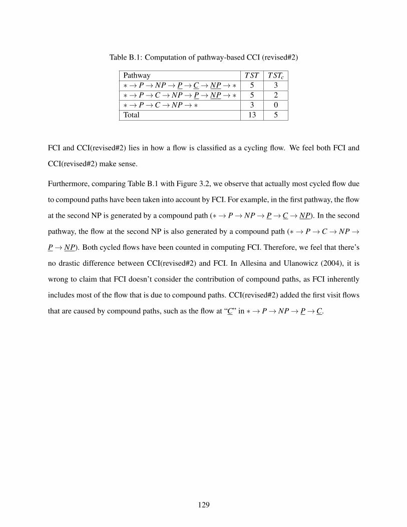
Table B.1: Computation of pathway-based CCI (revised#2)

Pathway T ST T STc∗→ P→ NP→ P→C→ NP→∗ 5 3∗→ P→C→ NP→ P→ NP→∗ 5 2∗→ P→C→ NP→∗ 3 0Total 13 5

FCI and CCI(revised#2) lies in how a flow is classified as a cycling flow. We feel both FCI and

CCI(revised#2) make sense.

Furthermore, comparing Table B.1 with Figure 3.2, we observe that actually most cycled flow due

to compound paths have been taken into account by FCI. For example, in the first pathway, the flow

at the second NP is generated by a compound path (∗→ P→ NP→ P→C→ NP). In the second

pathway, the flow at the second NP is also generated by a compound path (∗ → P→C→ NP→

P→ NP). Both cycled flows have been counted in computing FCI. Therefore, we feel that there’s

no drastic difference between CCI(revised#2) and FCI. In Allesina and Ulanowicz (2004), it is

wrong to claim that FCI doesn’t consider the contribution of compound paths, as FCI inherently

includes most of the flow that is due to compound paths. CCI(revised#2) added the first visit flows

that are caused by compound paths, such as the flow at “C” in ∗→ P→ NP→ P→C.

129

C. Non-uniqueness of Ulanowicz (1983)’s calculation of cycling

Ulanowicz (1983) quantifies cycling initially by identifying all the simple cycles. However, in

some cases, his method can produce multiple different cycling values for the same network. We

use a simple three-compartment network in Figure C.1 to demonstrate this issue. Ulanowicz (1983)

first uses a backtracking search algorithm to exhaustively enumerate all the simple cycles in the

network. In this example, without using the searching algorithm, we can easily find the three simple

cycles: two two-compartment cycles and one three-compartment cycle. As shown in Figure C.1,

three cycles are numbered from 1 to 3.

The next step is to attach a quantity of flow to each cycle. This is not a straightforward task. Some

preliminary works, such as finding out critical arc and computing circuit probability, are needed.

In each simple cycle, various arcs are different in magnitude. Critical arc is the one with smallest

flow. The circuit probability of a cycle is the probability that a quantum of medium starting at any

point in the given cycle will follow the simple pathway prescribed by the cycle to its starting point.

Take cycle 1 in Figure C.1 for example, the total output at A is 3, the probability the material in A

will flow to B (P(A→ B)) is 1/3. Similarly, P(B→ A) = 1/2. Thus the circuit probability for this

cycle P(Cycle 1) is the product of P(A→ B) and P(B→ A): 1/6. Utilizing the same procedure, the

circuit probabilities for the other two cycles are calculated as: P(Cycle 2) = 1/4 and P(Cycle 3) =

1/12.

If the cycles do not overlap, one can identify the critical arc in each cycle and subtract the mag-

nitude of that critical arc from each link in the cycle. However, in most cases, cycles do overlap:

several cycles may share the same critical arc. If this occurs, the smallest critical arc of all is

then identified and its value is divided among all those cycles in which it appears in proportion to

their respective circuit probabilities. These cycles sharing the smallest critical arc are then sub-

130

A

C  

B 11

1

Cycle  1  

A

C  

B 1

2

1

11

1

1

1

A

B1

1

C  

B1

1Cycle  2  

Cycle  3  

P(Cycle  1)=1/6  

P(Cycle  2)=1/4  

P(Cycle  3)=1/12  

Figure C.1: Three-compartment network and its three cycles

tracted. The set of critical arcs in the reminder network is reevaluated, and the subtraction process

is iterated until all cycles have been removed.

In this simple three-compartment network (Figure C.1), we find two critical arcs shared by more

than one cycles. One is the arc B→ A, which is shared by cycle 1 and cycle 3, and the other one is

C→ B, shared by cycle 2 and 3. Coincidentally, these two critical arcs have the same flow value

of 1. As the flows of two critical arcs are the same, we can start subtracting cycles with either one.

Option 1: start with arc B→ A. cycle 1 and cycle 3 are firstly subtracted from the network. These

two cycles split the 1 unit flow in arc B→ A in proportion to their circuit probabilities, which is

1/6 : 1/12 = 2:1. Thus, the weight for cycle 1 and 2 are 2/3 unit and 1/3 unit, respectively. Then,

subtract the last cycle 2 from the network. The top row in Figure C.2 shows the subtracted cycles

and reminder acyclic network. The sum of flows in three cycles is 23×2+ 1

3×3+ 23×2= 11

3 ≈ 3.67.

As the total number of flows for all arcs in this network is 9, the proportion of cycled flow over

total is 3.67/9 = 40.74%

131

A

B2/3  

2/3  

C  

B2/3  

2/3  + +

Op+on  1  A

C  

B 1/3  

1/3  

1/3  

+

A

C  

B 2/3  

2

1/3  

1

1/3  

1

A

B3/4  

3/4  

C  

B3/4  

3/4   + +

Op+on  2  A

C  

B 1/4  

1/4  

1/4  

+

A

C  

B 3/4  

2

1/4  

1

1/4  

1

Figure C.2: Two results of decomposing the network

Option 2: start with arc C→ B. Cycle 2 and cycle 3 are firstly subtracted. Then cycle 1. The

bottom row in Figure C.2 shows the subtracted cycles and reminder acyclic network in this case.

The sum of flows in three cycles is 34 × 2+ 1

4 × 3+ 34 × 2 = 15

4 = 3.75. The proportion of cycled

flow over total is 3.75/9 = 41.67%.

By slightly changing the sequence of subtracting cycles, the amount of cycling calculated are

different. Although the difference in this simple example is not very significant, the issue revealed

in this simple example is not negligible. If the same issue occurs in a much larger and more

complex network, depending on a very small difference, the computation can go one way or the

other, which makes this a discontinuous measure.

The procedure Ulanowicz (1983) used to subtract cycles is to make sure no residual flow will

become negative and no cycles will remain in the reminder acyclic network. Without adopting his

method, we can subtract the cycles in the following two ways, as shown in Figure C.3. Both satisfy

132

A

B1

1

C  

B1

1

A

C  

B 11

1

+ +

+ CI=3/9  

CI=4/9  

A

C  

1

2

1

1

A

C  

B

2

1

1

1

1

Op0on  3  

Op0on  4  

Figure C.3: Another two results of decomposing the network

that no residual flow is negative and no cycles remain. The first one has CI = 4/9 = 44.44%. The

Second has CI = 3/9 = 33.33%. The difference is up to about 11.11%.

Although the author set some rules in subtracting the cycles, it still cannot 100% make sure the

uniqueness of the result. A well-defined cycling index should not give an uncertain result. There-

fore we feel this non-uniqueness issue is a flaw with Ulanowicz (1983)’s technique in quantifying

cycling.

133

D. Computations of forty system-wide measures

Structure-based measures:

1. #compartments (n): the total number of compartments in the system.

2. #links (m): the total number of connections among all compartments.

3. #SCC: the number of strongly connected components (Newman, 2009). SCC is a subset of

the compartments such that (i) every compartment in the subset has a path to every other and

(ii) the subset is not part of some larger set with the property that every compartment can

reach every other.

4. #big SCC: the number of SCCs that have more than one compartment.

5. Percent nodes in big SCC: the number of compartments participating in big SCCs.

6. Link density, or complexity: the average number of intercompartmental links (m) per com-

partment.

Link density =mn

7. Connectance over direct paths: the ratio of the number of direct links (m) to the number of

possible intercompartmental links.

Connectance over direct paths =mn2

8. Connectance over all paths: the ratio of the number of direct and indirect links to the number

of possible intercompartmental links. Two compartments, that are not directly connected,

may be linked through indirect paths.

134

9. Degree diversity: degree of a compartment (D) is the number links that connects to it. We

apply Shannon’s information measure to the degree of all compartments in an ecosystem

network.

Degree diversity =−∑

(Di

D.

)log(

Di

D.

)

Flow-based measures:

1. Total boundary input: the sum of flows entering the system. It equals total boundary output

at steady state.

Total boundary input =n

∑i=1

zi

2. Total internal flow: the sum of flow rate for intercompartmental flows.

Total internal flow =n

∑i=1

n

∑j=1

Fi j

3. Total system throughflow (TST): the sum of throughflow at all compartments in the system.

T ST =n

∑i=1

Ti

4. Mean throughflow: the average throughflow of all compartments.

Mean throughflow =T ST

n

5. Total system throughput (Ulanowicz, 2004): the sum of all the flows, including environmen-

tal input (y), environmental output (y) and intercompartmental flows (F).

Total system throughput =n

∑i=1

n

∑j=1

Fi j +n

∑i=1

zi +n

∑i=1

yi =n

∑i=1

n

∑j=1

GFi j

135

6. Average path length (Finn, 1976) (or Network aggradation (Ulanowicz et al., 2006)): the

average number of compartments a unit flow material passes through before exiting the sys-

tem.

Aggradation =T ST

Total boundary input

7. I/D throughflow (Ma and Kazanci, 2012a):

(ID

)throughflow

=

n∑

i=1

[(G2 +G3 + · · ·)T

]n∑

i=1(GT )

=

n∑

i=1[(N− I−G)T ]

n∑

i=1(GT )

(6.4)

8. IEI throughflow:

IEIthrough f low =I

I +D=

( ID

)through f low

1+( I

D

)through f low

(6.5)

9. FCI (Finn’s cycling index) (Finn, 1978): the fraction of the total system throughflow (T ST )

due to cycling (T STc).

FCI = T STcT ST = 1

T ST

n

∑i=1

TiNii−1

Nii(6.6)

10. Amplification: the number of Ni j (i 6= j) larger than 1.

11. Amplification percentage: the fraction of Ni j (i 6= j) larger than 1.

Amplification percentage =Ampli f ication

n(n−1)

12. Synergism (Patten, 1991): the ratio of sum of positive entries over the sum of negative entries

in the utility analysis matrix.

Synergism =∑(U+)

|∑(U−) |

where U+ (U−) represents the positive (negative) partition matrices of utility matrix (U).

136

13. Mutualism (Patten, 1991): the ratio of number of positive entries over the number of negative

entries in the mutual relations matrix.

Mutualism =∑sign(U+)

∑sign(U−)

14. Homogenization (Fath and Patten, 1999b; Fath, 2004): the ratio of coefficient of variation

(CV) of G and N. CV is defined as the ratio of the standard deviation to the mean. Homoge-

nization exceeds one, because action of the network makes flow distribution more uniform.

Homogenization =CV (G)

CV (N)=

sd(G)/mean(G)

sd(N)/mean(N)

It quantifies the action of the network making the flow distribution more uniform. Higher

values indicate that resources become well mixed by cycling in the network, giving rise to a

more homogeneous distribution of flow.

15. Throughflow diversity:

Throughflow diversity =−∑

(Ti

T.

)log(

Ti

T.

)

Flow diversity (H): MacArthur (1955) applied Shannon’s information measure to the flows

in an ecosystem network.

H =−k∑i, j

GFi j

GF..log

GFi j

GF..(6.7)

GF.. is the sum of GFi j over all combinations of i and j. Rutledge et al. (1976)Rutledge et al.

(1976) decompose H into two parts: H = AMI + Hc. Please refer to the next two explana-

tions for AMI and Hc. Average mutual information (AMI): the average mutual information

inherent in the flow structure. It quantifies the overall constraint in the system, or how tightly

137

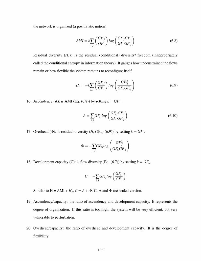
the network is organized (a positivistic notion)

AMI = k∑i, j

(GFi j

GF..

)log(

GFi jGF..GFi.GF. j

)(6.8)

Residual diversity (Hc): is the residual (conditional) diversity/ freedom (inappropriately

called the conditional entropy in information theory). It gauges how unconstrained the flows

remain or how flexible the system remains to reconfigure itself

Hc =−k∑i, j

(GFi j

GF..

)log

(GF2

i j

GFi.GF. j

)(6.9)

16. Ascendency (A): is AMI (Eq. (6.8)) by setting k = GF...

A = ∑i, j

GFi jlog(

GFi jGF..GFi.GF. j

)(6.10)

17. Overhead (Φ): is residual diversity (Hc) (Eq. (6.9)) by setting k = GF...

Φ =−∑i, j

GFi jlog

(GF2

i j

GFi.GF. j

)

18. Development capacity (C): is flow diversity (Eq. (6.7)) by setting k = GF...

C =−∑i, j

GFi jlog(

GFi j

GF..

)

Similar to H = AMI + Hc, C = A+Φ. C, A and Φ are scaled version.

19. Ascendency/capacity: the ratio of ascendency and development capacity. It represents the

degree of organization. If this ratio is too high, the system will be very efficient, but very

vulnerable to perturbation.

20. Overhead/capacity: the ratio of overhead and development capacity. It is the degree of

flexibility.

138

21. Internal ascendency (AI): is the ascendency generated solely by the internal flow between n

compartments.

AI = ∑i, j

Fi jlog(

Fi jF..Fi.F. j

)22. Internal overhead (ΦI): is the overhead generated solely by the internal flow between n

compartments.

ΦI =−∑i, j

Fi jlog

(F2

i j

Fi.F. j

)

23. Internal capacity (CI): is the development capacity generated solely by the internal flow

between n compartments.

CI =−∑i, j

Fi jlog(

Fi j

F..

)24. Robustness: characterizes the encounter between the opposing trends towards efficient oper-

ation (AMI/H) and increasing opportunity for re-configuration (-log(AMI/H))

Robustness =−eAMI

Hlog(

AMIH

)

where e is the based of natural logarithm.

25. Internal ascendency/capacity: the ratio of internal ascendency and internal development ca-

pacity.

26. Internal overhead/capacity: the ratio of internal overhead and internal development capacity.

Storage-based measures:

1. Total system storage (TSS): the sum of storage at all compartments in the system.

T SS =n

∑i=1

xi

139

2. Mean storage: the average storage of all compartments.

Mean storage =T SS

n

3. System residence time (system RT): the average time that flow material stay in the system.

System RT =T SS

Total boundary input

4. SCI (storage-based cycling index) (Ma and Kazanci, 2012b, in press 2014): the fraction of

total system storage (TSS) due to cycling (T SSc).

SCI =T SSc

T SS=

1T SS

n

∑i=1

xiSii−RTi

Sii=

1∑

ni=1 RTiTi

n

∑i=1

RTiTiNii−1

Nii(6.11)

5. Biomass diversity or information-theoretic biodiversity (D): MacArthur (1955) applied Shan-

non’s information measure to the storage values of all compartments in an ecosystem net-

work.

D =−∑

(xi

x.

)log(

xi

x.

)

140