pathtracing in practice - chalmers comp… · advanced computer graphics 2017 erik sintorn...
TRANSCRIPT
LIGHT TRANSPORTAdvanced Computer Graphics 2017
Erik Sintorn
1/25/2017 Advanced Computer Graphics – Light Transport 1

Before we start:
• Remember to choose a subject for your presentation
soon.
• And your project.
• Student representatives:
• JOHAN BACKMAN [email protected]
• KEVIN BJÖRKLUND [email protected]
• JONAS HULTÉN [email protected]
• HAMPUS LIDIN [email protected]
• VICTOR OLAUSSON [email protected]
• Come for a quick talk with me during recess.
• Muddy Cards!
1/25/2017 Advanced Computer Graphics - Path Tracing 2
Light Transport Simulation
• Rendering an image is a matter of ”simulating” how light
propagates through a virtual scene and lands on a virtual
camera film.
• Many algorithms exist, and the best one depends on
many factors.
• For a long time, Photon Mapping and Irradiance Caching
were extremely popular.
• Trade correctness for speed.
• Will cover these only very briefly.
1/25/2017 Advanced Computer Graphics - Path Tracing 3

Photon Mapping
Pinhole Camera
1/25/2017 Advanced Computer Graphics - Path Tracing 4
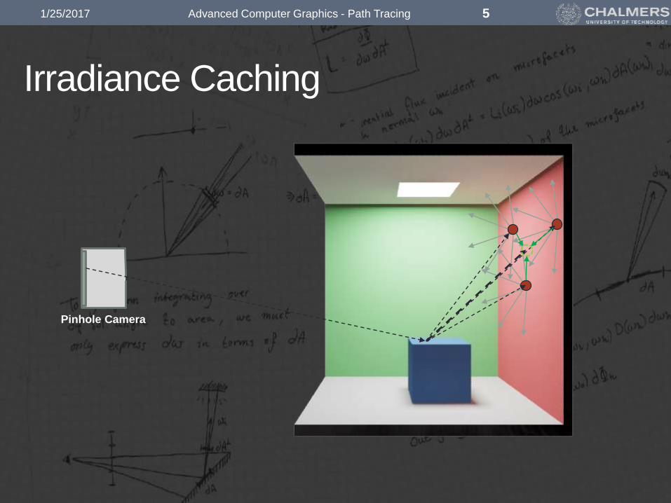
Irradiance Caching
Pinhole Camera
1/25/2017 Advanced Computer Graphics - Path Tracing 5

Path Tracing
• Path tracing is an algorithm for rendering images.
• Introduced by James Kajiya in 1986 as a numerical solution to the
Rendering Equation.
• The algorithm is convergent and unbiased.
• Has long been considered too noisy/slow to be used in industry.
• Today, almost all commercial renderers use some form of
unbiased pathtracing (at least optionally).
• Pixar (for example) only switched completely very recently.
• Why the sudden popularity?
1/25/2017 Advanced Computer Graphics - Path Tracing 6

Mental Ray (photon mapping) 32s
1/25/2017 Advanced Computer Graphics - Path Tracing 7
iRay (path tracing) 32s

1/25/2017 Advanced Computer Graphics - Path Tracing 8
iRay (path tracing) 2m8sMental Ray (photon mapping) 2m8s

1/25/2017 Advanced Computer Graphics - Path Tracing 9
iRay (path tracing) 2m8sMental Ray (photon mapping) 2m8s iRay (path tracing) ~1h

1/25/2017 Advanced Computer Graphics - Path Tracing 10
iRay (path tracing) 15mMental Ray 15m, 100M Photons, FG 1.0
• Artifacts never go away
• Scene specific tuning choices
• Immediate response
• Much easier to parallelize

Where does an image come from?
Pinhole Camera
1/25/2017 Advanced Computer Graphics - Path Tracing 11
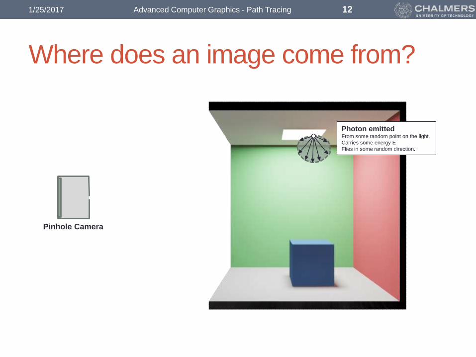
Where does an image come from?
Pinhole Camera
Photon emittedFrom some random point on the light.
Carries some energy E
Flies in some random direction.
1/25/2017 Advanced Computer Graphics - Path Tracing 12
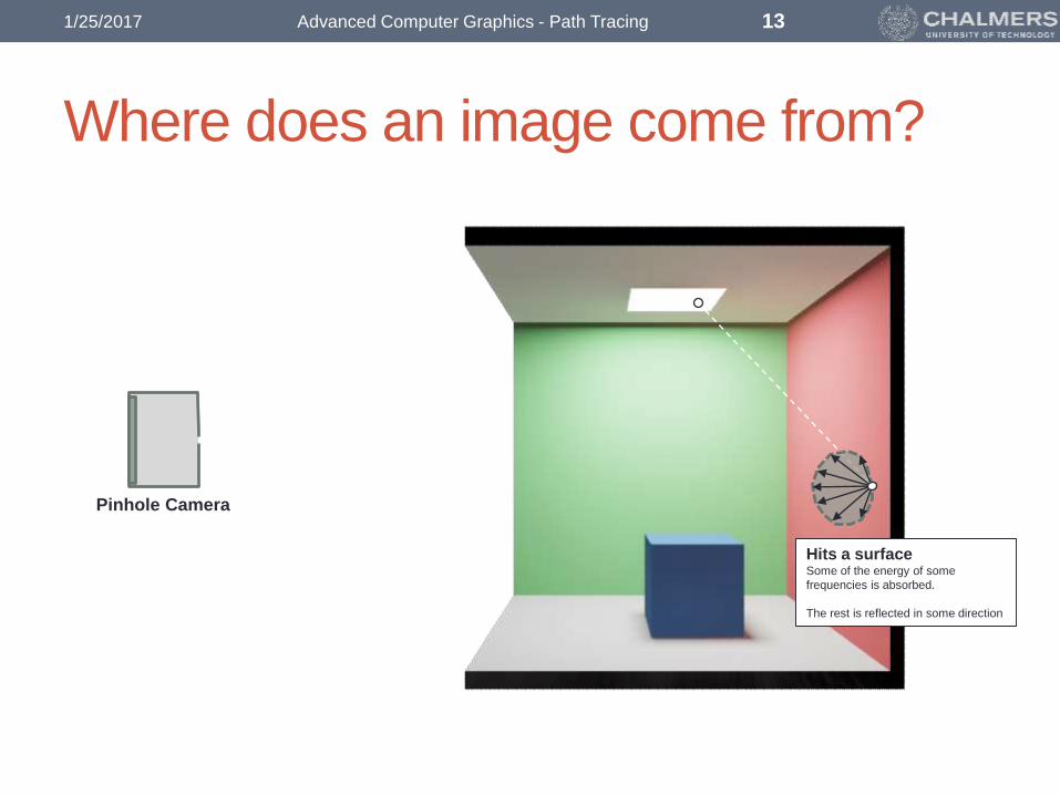
Where does an image come from?
Pinhole Camera
Hits a surfaceSome of the energy of some
frequencies is absorbed.
The rest is reflected in some direction
1/25/2017 Advanced Computer Graphics - Path Tracing 13

Where does an image come from?
Pinhole Camera
1/25/2017 Advanced Computer Graphics - Path Tracing 14
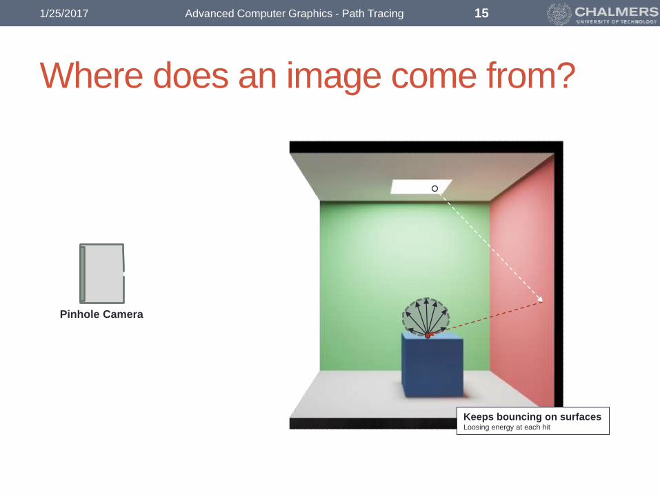
Where does an image come from?
Pinhole Camera
Keeps bouncing on surfacesLoosing energy at each hit
1/25/2017 Advanced Computer Graphics - Path Tracing 15

Where does an image come from?
Pinhole Camera
Until it leaves the scene…Or just runs out of energy
1/25/2017 Advanced Computer Graphics - Path Tracing 16
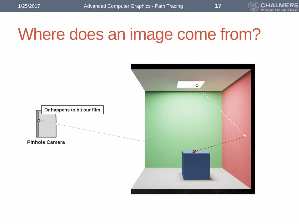
Where does an image come from?
Pinhole Camera
Or happens to hit our film
1/25/2017 Advanced Computer Graphics - Path Tracing 17

Light Transport Equation
𝑳𝒐 𝒑,𝝎 ?
𝝎𝒑
Radiance:
𝑾/(𝒎𝟐𝒔𝒓)
𝐿𝑜 𝒑,𝜔 = 𝐿𝑒 𝒑,𝜔 + න
Ω
𝑓 𝒑, 𝜔, 𝜔′ 𝐿𝑖 𝒑,𝜔′ cos 𝒏, 𝜔′ 𝑑𝜔′
1/25/2017 Advanced Computer Graphics - Path Tracing 18

Emitted radiance
Reflected radiance
Light Transport Equation
𝐿𝑜 𝒑,𝜔 = 𝐿𝑒 𝒑,𝜔 + න
Ω
𝑓 𝒑, 𝜔, 𝜔′ 𝐿𝑖 𝒑,𝜔′ cos 𝒏, 𝜔′ 𝑑𝜔′
𝜔𝒑
1/25/2017 Advanced Computer Graphics - Path Tracing 19

Emitted radiance
Reflected radiance
Light Transport Equation
𝐿𝑜 𝒑,𝜔 = 𝐿𝑒 𝒑,𝜔 + න
Ω
𝑓 𝒑, 𝜔, 𝜔′ 𝐿𝑖 𝒑,𝜔′ cos 𝒏, 𝜔′ 𝑑𝜔′
𝜔𝒑
Integrate over all
directions 𝜔′ in the
hemisphere around 𝒑
𝜔′
1/25/2017 Advanced Computer Graphics - Path Tracing 20

Emitted radiance
Reflected radiance
𝐿𝑜 𝒑,𝜔 = 𝐿𝑒 𝒑,𝜔 + න
Ω
𝑓 𝒑, 𝜔, 𝜔′ 𝐿𝑖 𝒑,𝜔′ cos 𝒏, 𝜔′ 𝑑𝜔′
Light Transport Equation
𝜔𝒑
Integrate over all
directions 𝜔′ in the
hemisphere around 𝒑
𝜔′
The radiance
incoming to point 𝒑from direction 𝜔′
𝐿𝑖 𝒑, 𝜔′
1/25/2017 Advanced Computer Graphics - Path Tracing 21

Emitted radiance
Reflected radiance
𝐿𝑜 𝒑,𝜔 = 𝐿𝑒 𝒑,𝜔 + න
Ω
𝑓 𝒑, 𝜔, 𝜔′ 𝐿𝑖 𝒑,𝜔′ cos 𝒏, 𝜔′ 𝑑𝜔′
Light Transport Equation
𝜔𝒑
Integrate over all
directions 𝜔′ in the
hemisphere around 𝒑
𝜔′
The radiance
incoming to point 𝒑from direction 𝜔′
𝐿𝑖 𝒑, 𝜔′
Convert between
irradiance parallel to 𝜔and irradiance on surface.
𝛼𝛼
1m2
𝜔′
𝒏cos 𝒏,𝜔′
1/25/2017 Advanced Computer Graphics - Path Tracing 22
Emitted radiance
Reflected radiance
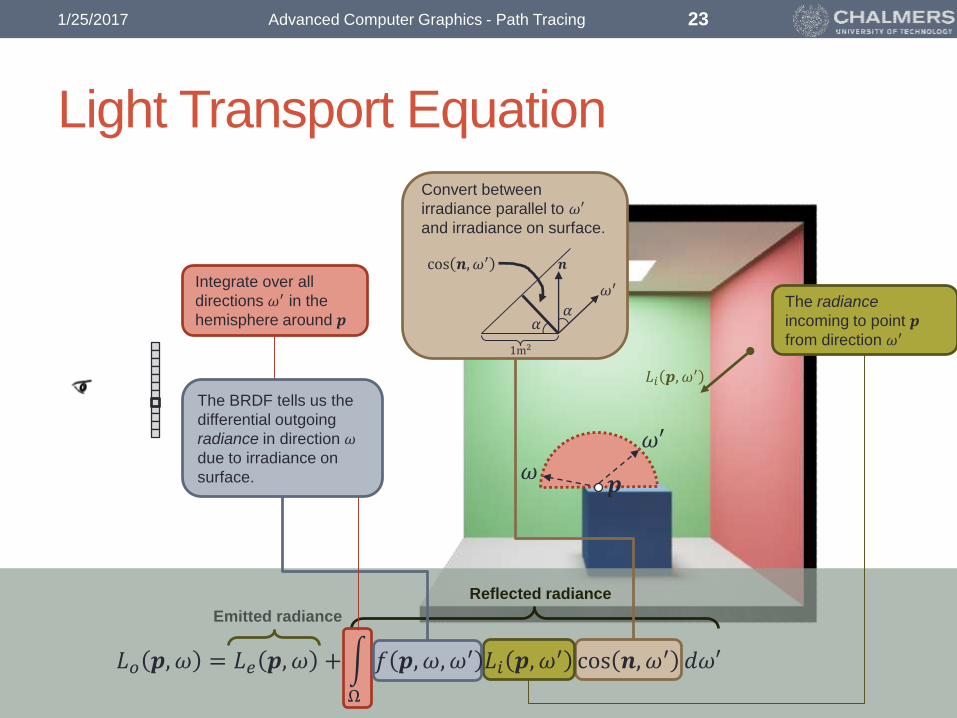
Light Transport Equation
𝜔𝒑
Integrate over all
directions 𝜔′ in the
hemisphere around 𝒑
𝜔′
The radiance
incoming to point 𝒑from direction 𝜔′
𝐿𝑖 𝒑, 𝜔′
Convert between
irradiance parallel to 𝜔′and irradiance on surface.
𝛼𝛼
1m2
𝜔′
𝒏cos 𝒏,𝜔′
𝐿𝑜 𝒑,𝜔 = 𝐿𝑒 𝒑,𝜔 + න
Ω
𝑓 𝒑, 𝜔, 𝜔′ 𝐿𝑖 𝒑,𝜔′ cos 𝒏, 𝜔′ 𝑑𝜔′
The BRDF tells us the
differential outgoing
radiance in direction 𝜔due to irradiance on
surface.
1/25/2017 Advanced Computer Graphics - Path Tracing 23

Emitted radiance
Reflected radiance
𝐿𝑜 𝒑,𝜔 = 𝐿𝑒 𝒑,𝜔 + න
Ω
𝑓 𝒑, 𝜔, 𝜔′ 𝐿𝑖 𝒑,𝜔′ cos 𝒏, 𝜔′ 𝑑𝜔′
Light Transport Equation
𝜔𝒑
𝜔′
−𝜔′
𝒑′
𝐿𝑖 𝒑,𝜔′ 𝐿𝑜 𝒑′, −𝜔′=
𝐿𝑒 𝒑′, −𝜔′ + න
Ω
𝑓 𝒑′, −𝜔′, 𝜔′′ 𝐿𝑖 𝒑′, 𝜔′ cos 𝒏′, 𝜔′ 𝑑𝜔′=
1/25/2017 Advanced Computer Graphics - Path Tracing 24

Numerical Integration
Area =0𝑋𝑓 𝑥 𝑑𝑥
0X
4
0
𝑓(𝑥)
𝑋
𝑁
𝑥
1/25/2017 Advanced Computer Graphics - Path Tracing 25
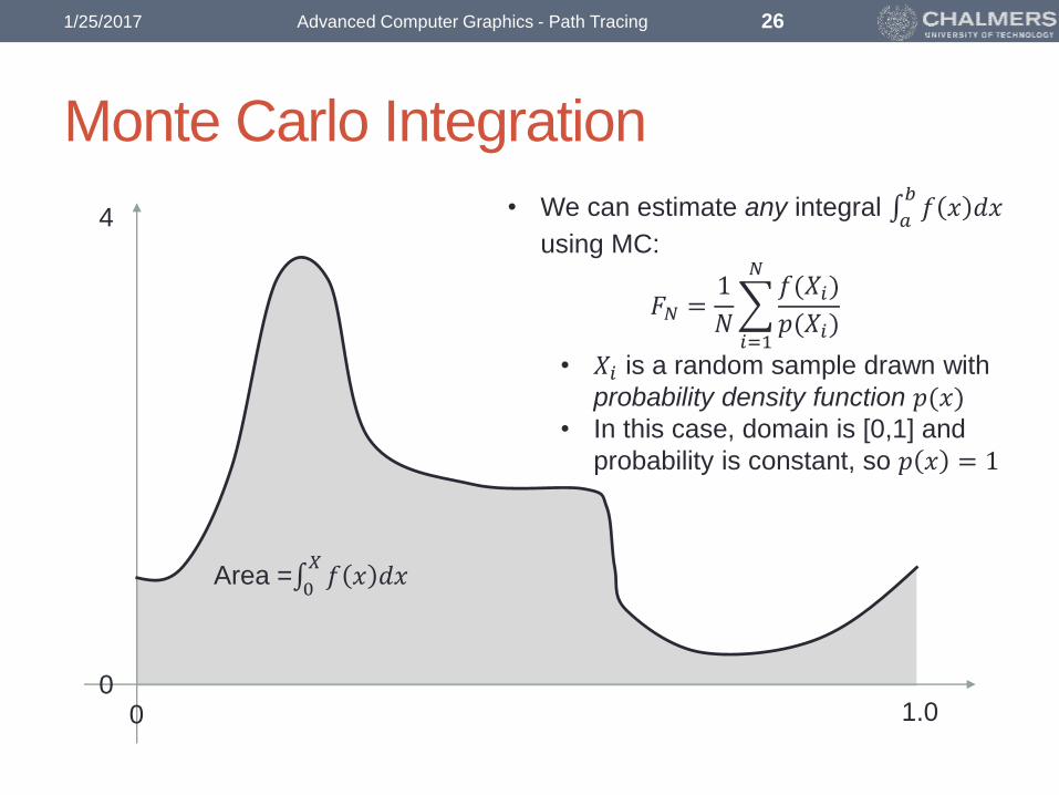
Monte Carlo Integration
Area =0𝑋𝑓 𝑥 𝑑𝑥
01.0
4
0
• We can estimate any integral 𝑎𝑏𝑓 𝑥 𝑑𝑥
using MC:
𝐹𝑁 =1
𝑁
𝑖=1
𝑁𝑓(𝑋𝑖)
𝑝(𝑋𝑖)
• 𝑋𝑖 is a random sample drawn with
probability density function 𝑝(𝑥)• In this case, domain is [0,1] and
probability is constant, so 𝑝 𝑥 = 1
1/25/2017 Advanced Computer Graphics - Path Tracing 26
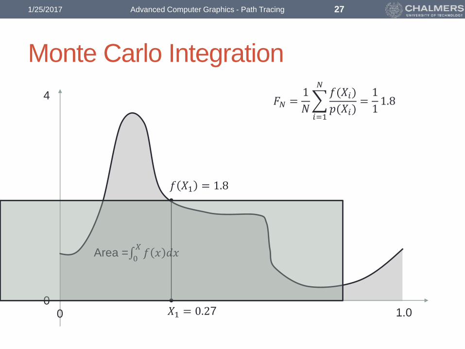
Monte Carlo Integration
Area =0𝑋𝑓 𝑥 𝑑𝑥
01.0
4
0
𝑓 𝑋1 = 1.8
𝑋1 = 0.27
𝐹𝑁 =1
𝑁
𝑖=1
𝑁𝑓(𝑋𝑖)
𝑝(𝑋𝑖)=1
11.8
1/25/2017 Advanced Computer Graphics - Path Tracing 27

Monte Carlo Integration
Area =0𝑋𝑓 𝑥 𝑑𝑥
01.0
4
0
𝑓 𝑋1 = 1.8
𝑋1 = 0.27
𝐹𝑁 =1
𝑁
𝑖=1
𝑁𝑓(𝑋𝑖)
𝑝(𝑋𝑖)=1
11.8
Convergent:As N approaches infinity, 𝐹𝑁 approaches 0
𝑋𝑓 𝑥 𝑑𝑥
Unbiased:
Regardless of N, the expected value 𝐸[𝐹𝑁] = 0𝑋𝑓 𝑥 𝑑𝑥 .
Which means that just averaging the results of an infinite number of
bad approximations will yield the correct value!
1/25/2017 Advanced Computer Graphics - Path Tracing 28

Monte Carlo Integration
Area =0𝑋𝑓 𝑥 𝑑𝑥
01.0
4
0
𝑓 𝑋1 = 1.8
𝑋1 = 0.27
𝐹𝑁 =1
𝑁
𝑖=1
𝑁𝑓(𝑋𝑖)
𝑝(𝑋𝑖)=1
3(1.8 + 1.0 + 0.2)
𝑓 𝑋2 = 1.0
𝑋2 = 0.05
𝑓 𝑋3 = 0.2
𝑋3 = 0.8
1/25/2017 Advanced Computer Graphics - Path Tracing 29
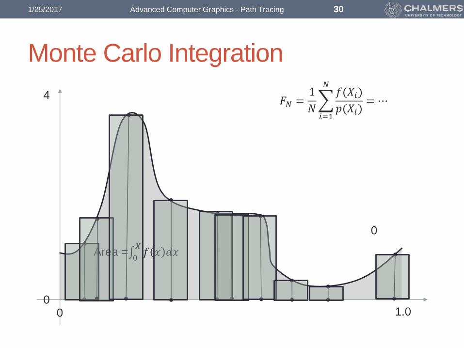
Monte Carlo Integration
Area =0𝑋𝑓 𝑥 𝑑𝑥
01.0
4
0
𝐹𝑁 =1
𝑁
𝑖=1
𝑁𝑓(𝑋𝑖)
𝑝(𝑋𝑖)= ⋯
0
1/25/2017 Advanced Computer Graphics - Path Tracing 30

Monte Carlo Integration
Area =0𝑋𝑓 𝑥 𝑑𝑥
01.0
4
0
𝐹𝑁 =1
𝑁
𝑖=1
𝑁𝑓(𝑋𝑖)
𝑝(𝑋𝑖)= ⋯4
1/25/2017 Advanced Computer Graphics - Path Tracing 31
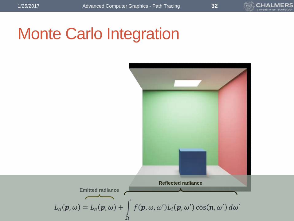
Emitted radiance
Reflected radiance
Monte Carlo Integration
1/25/2017 Advanced Computer Graphics - Path Tracing 32
𝐿𝑜 𝒑,𝜔 = 𝐿𝑒 𝒑,𝜔 + න
Ω
𝑓 𝒑, 𝜔, 𝜔′ 𝐿𝑖 𝒑,𝜔′ cos 𝒏, 𝜔′ 𝑑𝜔′

Emitted radiance
Reflected radiance
𝐿𝑜 𝒑, 𝜔 ≈ 𝐿𝑒 𝒑, 𝜔 +1
𝑁
𝑖=0
𝑁𝑓 𝒑, 𝜔, 𝜔𝑖 𝐿𝑖 𝒑,𝜔𝑖 cos 𝒏, 𝜔𝑖
𝑝(𝜔𝑖)
Monte Carlo Integration
1/25/2017 Advanced Computer Graphics - Path Tracing 33
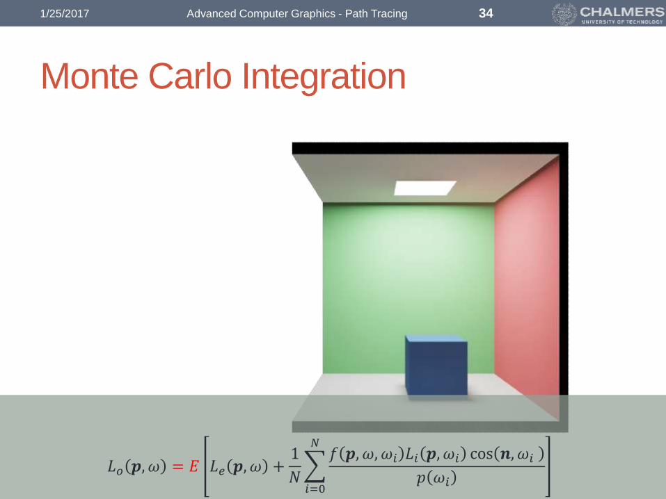
𝐿𝑜 𝒑,𝜔 = 𝐸 𝐿𝑒 𝒑,𝜔 +1
𝑁
𝑖=0
𝑁𝑓 𝒑, 𝜔, 𝜔𝑖 𝐿𝑖 𝒑,𝜔𝑖 cos 𝒏, 𝜔𝑖
𝑝 𝜔𝑖
Monte Carlo Integration
1/25/2017 Advanced Computer Graphics - Path Tracing 34

𝐿𝑜 𝒑,𝜔 = 𝐸 𝐿𝑒 𝒑,𝜔 +1
1
𝑖=0
1𝑓 𝒑, 𝜔, 𝜔𝑖 𝐿𝑖 𝒑,𝜔𝑖 cos 𝒏, 𝜔𝑖
𝑝 𝜔𝑖
Sample hemisphere
uniformly :
𝑝 𝜔𝑖 =1
2𝜋
Monte Carlo Integration
1/25/2017 Advanced Computer Graphics - Path Tracing 35

Monte Carlo Integration
𝐿𝑜 𝒑, 𝜔 = 𝐸 𝐿𝑒 𝒑,𝜔 +𝑓 𝒑,𝜔, 𝜔𝑖 𝐿𝑖 𝒑,𝜔𝑖 cos 𝒏, 𝜔𝑖
𝑝 𝜔𝑖
Sample hemisphere
uniformly :
𝑝 𝜔𝑖 =1
2𝜋
1/25/2017 Advanced Computer Graphics - Path Tracing 36
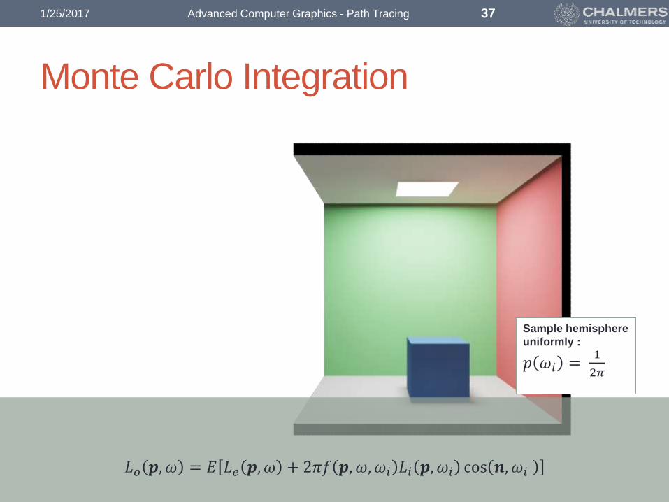
Monte Carlo Integration
𝐿𝑜 𝒑,𝜔 = 𝐸 𝐿𝑒 𝒑,𝜔 + 2𝜋𝑓 𝒑,𝜔, 𝜔𝑖 𝐿𝑖 𝒑,𝜔𝑖 cos 𝒏, 𝜔𝑖
Sample hemisphere
uniformly :
𝑝 𝜔𝑖 =1
2𝜋
1/25/2017 Advanced Computer Graphics - Path Tracing 37
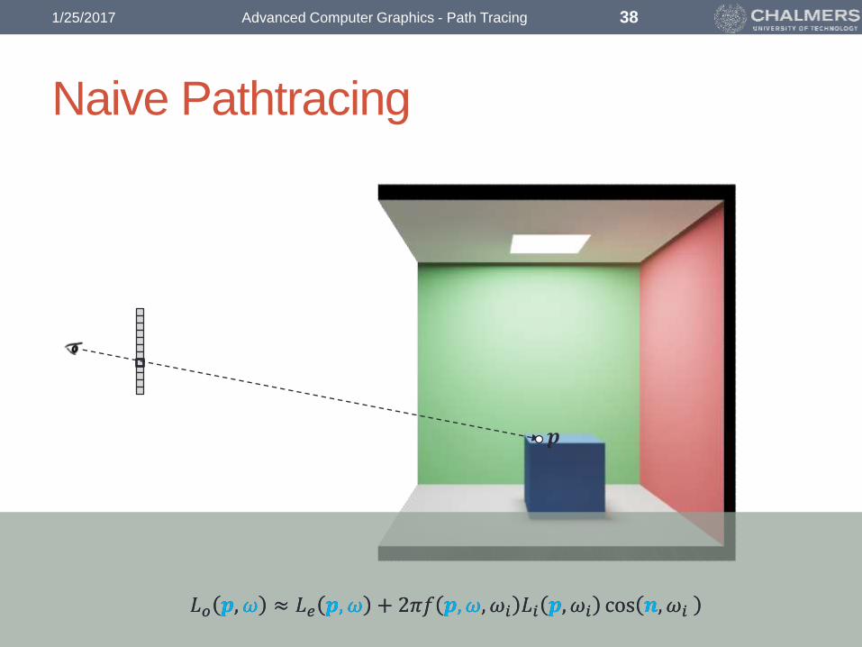
Naive Pathtracing
𝐿𝑜 𝒑, 𝜔 ≈ 𝐿𝑒 𝒑, 𝜔 + 2𝜋𝑓 𝒑,𝜔, 𝜔𝑖 𝐿𝑖 𝒑,𝜔𝑖 cos 𝒏, 𝜔𝑖
𝒑
𝐿𝑜 𝒑, 𝜔 ≈ 𝐿𝑒 𝒑, 𝜔 + 2𝜋𝑓 𝒑,𝜔, 𝜔𝑖 𝐿𝑖 𝒑,𝜔𝑖 cos 𝒏, 𝜔𝑖
1/25/2017 Advanced Computer Graphics - Path Tracing 38

Naive Pathtracing
𝒑
𝜔𝑖
𝐿𝑜 𝒑, 𝜔 ≈ 𝐿𝑒 𝒑, 𝜔 + 2𝜋𝑓 𝒑,𝜔, 𝜔𝑖 𝐿𝑖 𝒑,𝜔𝑖 cos 𝒏, 𝜔𝑖𝐿𝑜 𝒑, 𝜔 ≈ 𝐿𝑒 𝒑, 𝜔 + 2𝜋𝑓 𝒑,𝜔, 𝜔𝑖 𝐿𝑖 𝒑,𝜔𝑖 cos 𝒏, 𝜔𝑖𝐿𝑜 𝒑, 𝜔 ≈ 𝐿𝑒 𝒑, 𝜔 + 2𝜋𝑓 𝒑,𝜔, 𝜔𝑖 𝐿𝑖 𝒑,𝜔𝑖 cos 𝒏, 𝜔𝑖
1/25/2017 Advanced Computer Graphics - Path Tracing 39
Naive Pathtracing
𝒑
𝜔𝑖
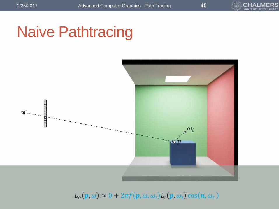
𝐿𝑜 𝒑,𝜔 ≈ 0 + 2𝜋𝑓 𝒑,𝜔, 𝜔𝑖 𝐿𝑖 𝒑,𝜔𝑖 cos 𝒏, 𝜔𝑖
1/25/2017 Advanced Computer Graphics - Path Tracing 40

Naive Pathtracing
𝐿𝑜 𝒑,𝜔 ≈ 0 + 2𝜋𝑓 𝒑,𝜔, 𝜔𝑖 𝐿𝑜 𝒑′, −𝜔𝑖 cos 𝒏, 𝜔𝑖
𝒑
𝜔𝑖
𝒑′
1/25/2017 Advanced Computer Graphics - Path Tracing 41

Naive Pathtracing
𝒑
𝜔𝑖
𝒑′
𝐿𝑜 𝒑,𝜔 ≈ 0 + 2𝜋𝑓 𝒑,𝜔, 𝜔𝑖 𝐿𝑖 𝒑,𝜔𝑖 cos 𝒏, 𝜔𝑖
1/25/2017 Advanced Computer Graphics - Path Tracing 42

Naive Pathtracing
𝐿𝑜 𝒑,𝜔 ≈ 0 + 2𝜋𝑓 𝒑,𝜔,𝜔𝑖 𝐿𝑒 𝒑′, −𝜔𝑖 + 2𝜋𝑓 𝒑′, −𝜔𝑖 , 𝜔𝑗 𝐿𝑖 𝒑′,𝜔𝑗 cos 𝒏′, 𝜔𝑗 cos 𝒏, 𝜔𝑖
𝒑
𝜔𝑖
𝒑′
1/25/2017 Advanced Computer Graphics - Path Tracing 43

Naive Pathtracing
𝐿𝑜 𝒑,𝜔 ≈ 0 + 2𝜋𝑓 𝒑,𝜔, 𝜔𝑖 0 + 2𝜋𝑓 𝒑′, −𝜔𝑖 , 𝜔𝑗 𝐿𝑖 𝒑′, 𝜔𝑗 cos 𝒏′, 𝜔𝑗 cos 𝒏, 𝜔𝑖
𝒑
𝜔𝑖
𝒑′
𝜔𝑗
1/25/2017 Advanced Computer Graphics - Path Tracing 44

Naive Pathtracing
𝐿𝑜 𝒑,𝜔 ≈ 0 + 2𝜋𝑓 𝒑,𝜔, 𝜔𝑖 0 + 2𝜋𝑓 𝒑′, −𝜔𝑖 , 𝜔𝑗 𝐿𝑖 𝒑′, 𝜔𝑗 cos 𝒏′, 𝜔𝑗 cos 𝒏, 𝜔𝑖
𝒑
𝜔𝑖
𝒑′
𝜔𝑗
𝒑′
1/25/2017 Advanced Computer Graphics - Path Tracing 45

Naive Pathtracing
𝐿𝑜 𝒑,𝜔 ≈ 0 + 2𝜋𝑓 𝒑,𝜔, 𝜔𝑖 0 + 2𝜋𝑓 𝒑′, −𝜔𝑖 , 𝜔𝑗 𝐿𝑜 𝒑′′, −𝜔𝑗 cos 𝒏′, 𝜔𝑗 cos 𝒏, 𝜔𝑖
𝒑
𝜔𝑖
𝒑′
𝜔𝑗
𝒑′′
1/25/2017 Advanced Computer Graphics - Path Tracing 46

Naive Pathtracing
𝐿𝑜 𝒑,𝜔 ≈ 0 + 2𝜋𝑓 𝒑,𝜔, 𝜔𝑖 0 + 2𝜋𝑓 𝒑′, −𝜔𝑖 , 𝜔𝑗 𝐿𝑒 𝒑′′, −𝜔𝑖 cos 𝒏′, 𝜔𝑗 cos 𝒏, 𝜔𝑖
𝒑
𝜔𝑖
𝒑′
𝜔𝑗
𝒑′′
1/25/2017 Advanced Computer Graphics - Path Tracing 47

Naive Pathtracing
𝒑
𝜔𝑖
𝒑′
𝜔𝑗
𝒑′′
What’s so naïve about this?
1/25/2017 Advanced Computer Graphics - Path Tracing 48

Surface form of LTE
1/25/2017 Advanced Computer Graphics - Path Tracing 49

Separating Direct And Indirect Illumination
𝒑
𝐿𝑜 𝒑,𝜔 = න
𝐴
𝑓 𝒑, 𝒒 → 𝒑 𝐿𝑖 𝒑, 𝒒 → 𝒑 𝐺 𝒑, 𝒒 𝑉 𝒑, 𝒒 𝑑𝑨 + න
Ω
𝑓(𝒑,𝜔,𝜔′)𝐿𝑖(𝒑,𝜔′)cos(𝒏,𝜔′)𝑑𝜔′
direct illumination indirect illumination
𝒑′
𝒑′′
1/25/2017 Advanced Computer Graphics - Path Tracing 50

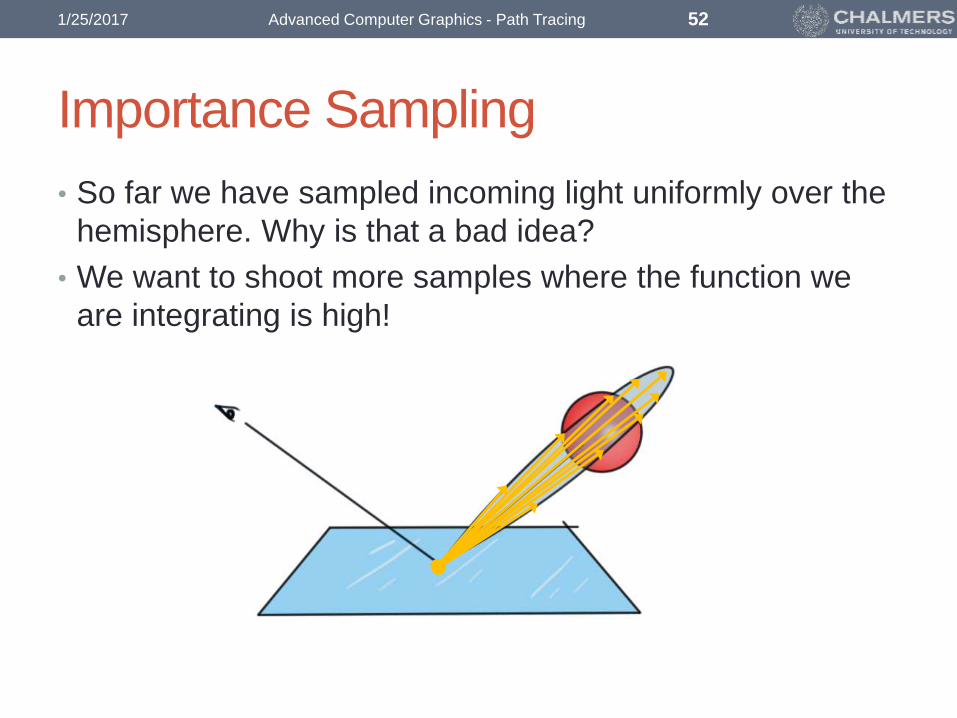
Importance Sampling
• So far we have sampled incoming light uniformly over the
hemisphere. Why is that a bad idea?
• We want to shoot more samples where the function we
are integrating is high!
1/25/2017 Advanced Computer Graphics - Path Tracing 51
Importance Sampling
• So far we have sampled incoming light uniformly over the
hemisphere. Why is that a bad idea?
• We want to shoot more samples where the function we
are integrating is high!
1/25/2017 Advanced Computer Graphics - Path Tracing 52
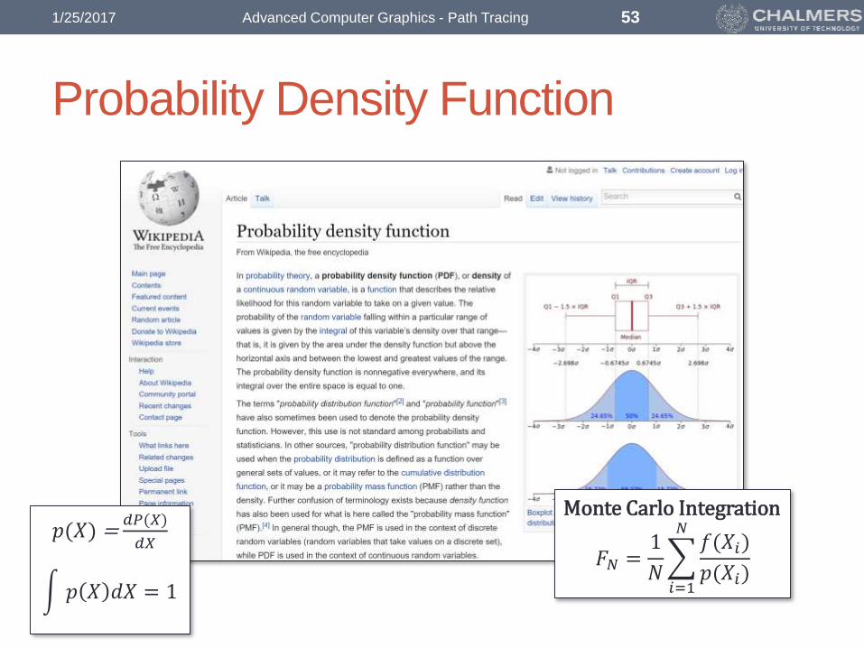
Probability Density Function
1/25/2017 Advanced Computer Graphics - Path Tracing 53
Monte Carlo Integration
𝐹𝑁 =1
𝑁
𝑖=1
𝑁𝑓(𝑋𝑖)
𝑝(𝑋𝑖)
𝑝(𝑋) = 𝑑𝑃(𝑋)
𝑑𝑋
න 𝑝 𝑋 𝑑𝑋 = 1

Importance Sampling
0 3
4
1 2
𝑝 𝑥 =1
3
1/25/2017 Advanced Computer Graphics - Path Tracing 54
Monte Carlo Integration
𝐹𝑁 =1
𝑁
𝑖=1
𝑁𝑓(𝑋𝑖)
𝑝(𝑋𝑖)
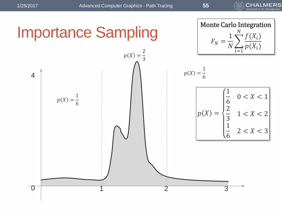
Importance Sampling
0 3
4
1 2
𝑝 𝑋 =
1
60 < 𝑋 < 1
2
31 < 𝑋 < 2
1
62 < 𝑋 < 3
𝑝 𝑋 =1
6
𝑝 𝑋 =2
3
𝑝 𝑋 =1
6
1/25/2017 Advanced Computer Graphics - Path Tracing 55
Monte Carlo Integration
𝐹𝑁 =1
𝑁
𝑖=1
𝑁𝑓(𝑋𝑖)
𝑝(𝑋𝑖)

Importance Sampling
0 3
4
1 2
𝑝 𝑋 =1
6
𝑝 𝑋 =2
3
𝑝 𝑋 =1
6
1/25/2017 Advanced Computer Graphics - Path Tracing 56
Monte Carlo Integration
𝐹𝑁 =1
𝑁
𝑖=1
𝑁𝑓(𝑋𝑖)
𝑝(𝑋𝑖)
𝑝 𝑋 =
1
60 < 𝑋 < 1
2
31 < 𝑋 < 2
1
62 < 𝑋 < 3

Importance Sampling
0 3
4
1 2
Example:
𝑝 𝑋 = 𝑎 𝑒(−
𝑥−1.5 2
2𝑐2)
1/25/2017 Advanced Computer Graphics - Path Tracing 57
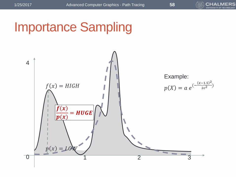
Importance Sampling
0 3
4
1 2
Example:
𝑝 𝑋 = 𝑎 𝑒(−
𝑥−1.5 2
2𝑐2)𝑓 𝑥 = 𝐻𝐼𝐺𝐻
𝑝 𝑥 = 𝐿𝑂𝑊
𝒇 𝒙
𝒑(𝒙)= 𝑯𝑼𝑮𝑬
1/25/2017 Advanced Computer Graphics - Path Tracing 58

1/25/2017 Advanced Computer Graphics - Path Tracing 59

1/25/2017 Advanced Computer Graphics - Path Tracing 60

1/25/2017 Advanced Computer Graphics - Path Tracing 61

1/25/2017 Advanced Computer Graphics - Path Tracing 62

1/25/2017 Advanced Computer Graphics - Path Tracing 63

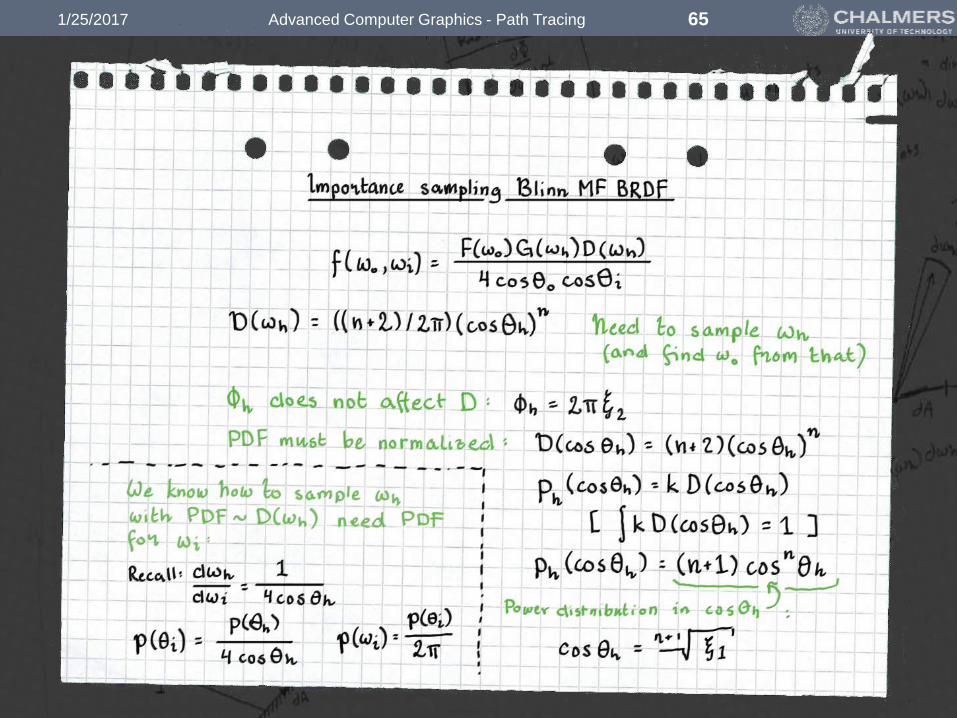
Importance Sampling
• When evaluating the
Rendering Equation, we do
not know the function we
want to integrate
• Since it depends on the
incoming light over the
hemisphere
• But we do know the BRDF, so
we importance sample on that
1/25/2017 Advanced Computer Graphics - Path Tracing 64
𝐿𝑜 𝒑,𝜔 = න
Ω
𝑓 𝒑,𝜔,𝜔′ 𝐿𝑖 𝒑,𝜔′ cos 𝒏,𝜔′ 𝑑𝜔′
1/25/2017 Advanced Computer Graphics - Path Tracing 65
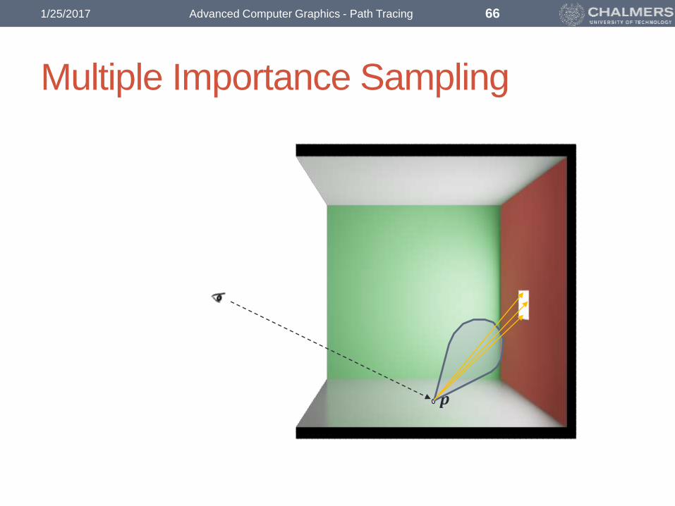
Multiple Importance Sampling
𝒑
1/25/2017 Advanced Computer Graphics - Path Tracing 66

Multiple Importance Sampling
𝒑
1/25/2017 Advanced Computer Graphics - Path Tracing 67
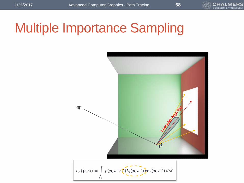
Multiple Importance Sampling
𝒑
1/25/2017 Advanced Computer Graphics - Path Tracing 68
𝐿𝑜 𝒑,𝜔 = න
Ω
𝑓 𝒑,𝜔,𝜔′ 𝐿𝑖 𝒑,𝜔′ cos 𝒏,𝜔′ 𝑑𝜔′

Multiple Importance Sampling
𝒑
1/25/2017 Advanced Computer Graphics - Path Tracing 69
𝐿𝑜 𝒑,𝜔 = න
Ω
𝑓 𝒑,𝜔,𝜔′ 𝐿𝑖 𝒑,𝜔′ cos 𝒏,𝜔′ 𝑑𝜔′
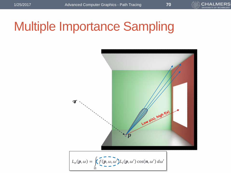
Multiple Importance Sampling
𝒑
1/25/2017 Advanced Computer Graphics - Path Tracing 70
𝐿𝑜 𝒑,𝜔 = න
Ω
𝑓 𝒑,𝜔,𝜔′ 𝐿𝑖 𝒑,𝜔′ cos 𝒏,𝜔′ 𝑑𝜔′

Multiple Importance Sampling
1/25/2017 Advanced Computer Graphics - Path Tracing 71
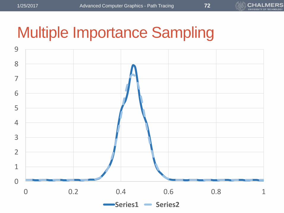
Multiple Importance Sampling
0
1
2
3
4
5
6
7
8
9
0 0.2 0.4 0.6 0.8 1
Series1 Series2
1/25/2017 Advanced Computer Graphics - Path Tracing 72

Multiple Importance Sampling
0
1
2
3
4
5
6
7
8
9
0 0.2 0.4 0.6 0.8 1
Series1 Series2 Series3
1/25/2017 Advanced Computer Graphics - Path Tracing 73

Multiple Importance Sampling
0
1
2
3
4
5
6
7
8
9
10
0 0.2 0.4 0.6 0.8 1
Series1 Series2 Series3 Series4
1/25/2017 Advanced Computer Graphics - Path Tracing 74

Multiple Importance Sampling
0
1
2
3
4
5
6
7
8
9
10
0 0.2 0.4 0.6 0.8 1
Series1 Series2 Series3 Series4 Series5
1/25/2017 Advanced Computer Graphics - Path Tracing 75

Multiple Importance Sampling
0
1
2
3
4
5
6
7
8
9
10
0 0.2 0.4 0.6 0.8 1
Series1 Series2 Series3 Series4 Series5
1/25/2017 Advanced Computer Graphics - Path Tracing 76
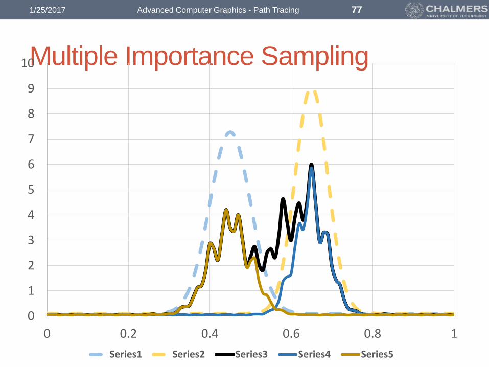
Multiple Importance Sampling
0
1
2
3
4
5
6
7
8
9
10
0 0.2 0.4 0.6 0.8 1
Series1 Series2 Series3 Series4 Series5
1/25/2017 Advanced Computer Graphics - Path Tracing 77

Multiple Importance Sampling
Need to estimate:
න𝑓 𝑥 𝑔 𝑥 𝑑𝑥
Could Use:
0.5𝑓 𝑋 𝑔 𝑋
𝑝𝑓 𝑋+
𝑓 𝑌 𝑔 𝑌
𝑝𝑔 𝑌?
1/25/2017 Advanced Computer Graphics - Path Tracing 78

Multiple Importance Sampling
Need to estimate:
න𝑓 𝑥 𝑔 𝑥 𝑑𝑥
Could Use:
0.5𝑓 𝑋 𝑔 𝑋
𝑝𝑓 𝑋+
𝑓 𝑌 𝑔 𝑌
𝑝𝑔 𝑌?
Better (MIS):
0.5𝑓 𝑋 𝑔 𝑋
0.5(𝑝𝑓 𝑋 + 𝑝𝑔(𝑋))+
𝑓 𝑌 𝑔 𝑌
0.5(𝑝𝑓 𝑌 + 𝑝𝑔(𝑌))
1/25/2017 Advanced Computer Graphics - Path Tracing 79

Multiple Importance Sampling
Need to estimate:
න𝑓 𝑥 𝑔 𝑥 𝑑𝑥
Could Use:
0.5𝑓 𝑋 𝑔 𝑋
𝑝𝑓 𝑋+
𝑓 𝑌 𝑔 𝑌
𝑝𝑔 𝑌?
Better (MIS):𝑓 𝑋 𝑔 𝑋
𝑝𝑓 𝑋 + 𝑝𝑔(𝑋)+
𝑓 𝑌 𝑔 𝑌
𝑝𝑓 𝑌 + 𝑝𝑔(𝑌)
1/25/2017 Advanced Computer Graphics - Path Tracing 80

Multiple Importance Sampling
0
1
2
3
4
5
6
7
8
9
10
0 0.2 0.4 0.6 0.8 1
Series1 Series2 Series3 Series4
1/25/2017 Advanced Computer Graphics - Path Tracing 81

Multiple Importance Sampling
0
1
2
3
4
5
6
7
8
9
10
0 0.2 0.4 0.6 0.8 1
Series1 Series2 Series3 Series4 Series5
1/25/2017 Advanced Computer Graphics - Path Tracing 82
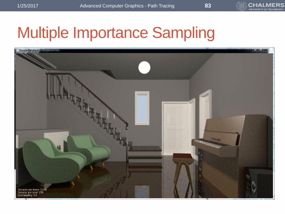
Multiple Importance Sampling
𝒑
Do both!
• Sample brdf first
• Then light
• PDF of this sampling strategy is (weighted) sum
• - Only very low if neither technique is likely to choose dir
1/25/2017 Advanced Computer Graphics - Path Tracing 83

Stratified Sampling
• Another standard variance reduction method
• When just choosing samples randomly over the domain,
they may “clump” and take
a long while to converge
It will converge to 0.5
after unlimited time.
But after four samples I still
have prob=1/8 that the pixel
will be considered all in shadow
or completely unshadowed
1/25/2017 Advanced Computer Graphics - Path Tracing 84

Stratified Sampling
• Divide domain into “strata”
• Don’t sample one strata again until
all others have been sampled
once.
1/25/2017 Advanced Computer Graphics - Path Tracing 85

Stratified Sampling
• If we know how many samples we want to take, we can
get good stratification from “jittering”
• If not, we want any sequence of samples to have good
stratification. We can use a Low Discrepancy Sequence
SOBOL: 100 samples SOBOL: 1000 samples SOBOL: 10000 samples RANDOM: 10000 samples
1/25/2017 Advanced Computer Graphics - Path Tracing 86
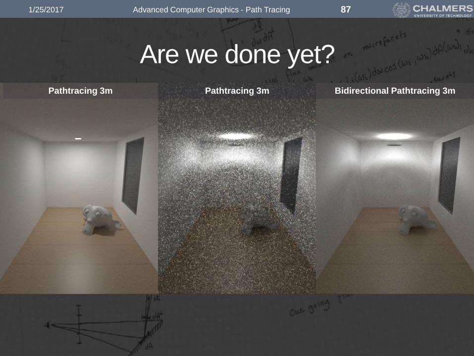
1/25/2017 Advanced Computer Graphics - Path Tracing 87
Pathtracing 3mPathtracing 3m Bidirectional Pathtracing 3m
Are we done yet?
1/25/2017 Advanced Computer Graphics - Path Tracing 88
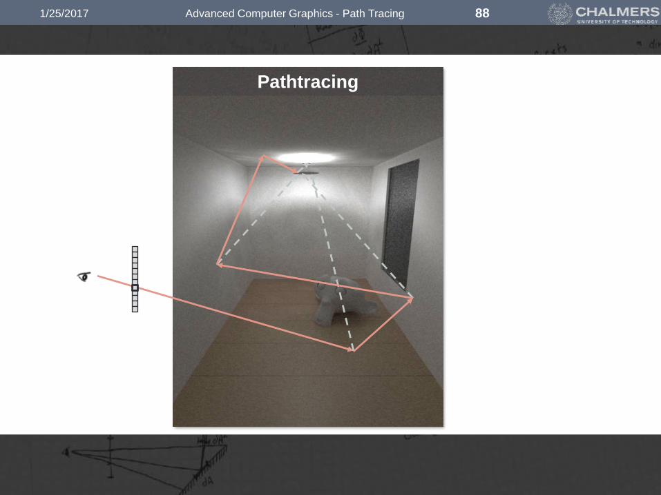
Pathtracing

1/25/2017 Advanced Computer Graphics - Path Tracing 89
Bidirectional Pathtracing
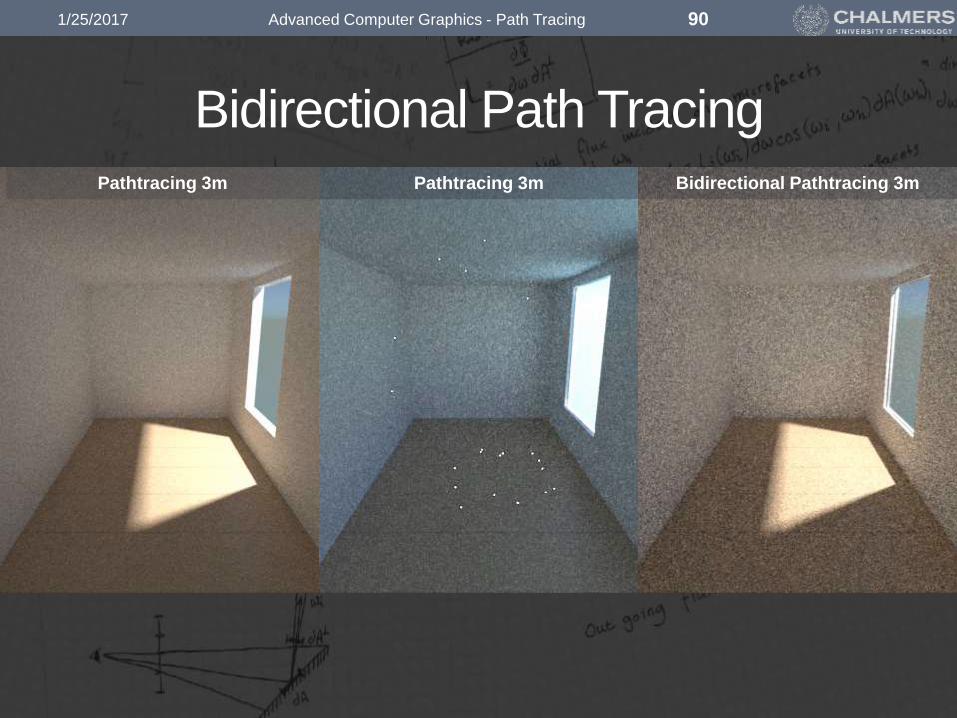
1/25/2017 Advanced Computer Graphics - Path Tracing 90
Pathtracing 3mPathtracing 3m Bidirectional Pathtracing 3m
Bidirectional Path Tracing

1/25/2017 Advanced Computer Graphics - Path Tracing 91
Pathtracing 75SPP (~5min) Bidirectional Pathtracing 45SPP (~5min)

1/25/2017 Advanced Computer Graphics - Path Tracing 92
Bidirectional Pathtracing 30mBidirectional Pathtracing 30m Metropolis Light Transport 30m
Are we done yet?

1/25/2017 Advanced Computer Graphics - Path Tracing 93
Metropolis Light Transport

1/25/2017 Advanced Computer Graphics - Path Tracing 94
Metropolis Light Transport

1/25/2017 Advanced Computer Graphics - Path Tracing 95
Metropolis Light Transport

BD 2hBD 5m BD 19h 4m 12240 SPP
Bidirectional Path Tracing
1/25/2017 Advanced Computer Graphics - Path Tracing 96

MLT 17h35m, 9300 SPPMLT 2hMLT 5m
Metropolis Light Transport
1/25/2017 Advanced Computer Graphics - Path Tracing 97

5min 25min 1h15min
Bidirectional Path Tracing
1/25/2017 Advanced Computer Graphics - Path Tracing 98

5min 25min 1h
Metropolis Light Transport
1/25/2017 Advanced Computer Graphics - Path Tracing 99

Further Reading
1/25/2017 Advanced Computer Graphics - Path Tracing 100
Pathtracing Lab