paths in graphs - university of california, berkeleyvazirani/algorithms/... · · 2006-10-03this...

Chapter 4

Paths in graphs

4.1 DistancesDepth-first search readily identifies all the vertices of a graph that can be reached from adesignated starting point. It also finds explicit paths to these vertices, summarized in itssearch tree (Figure 4.1). However, these paths might not be the most economical ones possi-ble. In the figure, vertex C is reachable from S by traversing just one edge, while the DFS treeshows a path of length 3. This chapter is about algorithms for finding shortest paths in graphs.

Path lengths allow us to talk quantitatively about the extent to which different vertices ofa graph are separated from each other:

The distance between two nodes is the length of the shortest path between them.

To get a concrete feel for this notion, consider a physical realization of a graph that has a ballfor each vertex and a piece of string for each edge. If you lift the ball for vertex s high enough,the other balls that get pulled up along with it are precisely the vertices reachable from s.And to find their distances from s, you need only measure how far below s they hang.

Figure 4.1 (a) A simple graph and (b) its depth-first search tree.

(a)

E AS

BD C

(b) S

A

B

D

E

C

115

116 Algorithms

Figure 4.2 A physical model of a graph.

B

E S

D C

A

S

D EC

B

A

In Figure 4.2 for example, vertex B is at distance 2 from S, and there are two shortestpaths to it. When S is held up, the strings along each of these paths become taut. On theother hand, edge (D,E) plays no role in any shortest path and therefore remains slack.

4.2 Breadth-first searchIn Figure 4.2, the lifting of s partitions the graph into layers: s itself, the nodes at distance1 from it, the nodes at distance 2 from it, and so on. A convenient way to compute distancesfrom s to the other vertices is to proceed layer by layer. Once we have picked out the nodesat distance 0, 1, 2, . . . , d, the ones at d+ 1 are easily determined: they are precisely the as-yet-unseen nodes that are adjacent to the layer at distance d. This suggests an iterative algorithmin which two layers are active at any given time: some layer d, which has been fully identified,and d+ 1, which is being discovered by scanning the neighbors of layer d.

Breadth-first search (BFS) directly implements this simple reasoning (Figure 4.3). Ini-tially the queue Q consists only of s, the one node at distance 0. And for each subsequentdistance d = 1, 2, 3, . . ., there is a point in time at which Q contains all the nodes at distanced and nothing else. As these nodes are processed (ejected off the front of the queue), theiras-yet-unseen neighbors are injected into the end of the queue.

Let’s try out this algorithm on our earlier example (Figure 4.1) to confirm that it does theright thing. If S is the starting point and the nodes are ordered alphabetically, they get visitedin the sequence shown in Figure 4.4. The breadth-first search tree, on the right, contains theedges through which each node is initially discovered. Unlike the DFS tree we saw earlier, ithas the property that all its paths from S are the shortest possible. It is therefore a shortest-path tree.

Correctness and efficiencyWe have developed the basic intuition behind breadth-first search. In order to check thatthe algorithm works correctly, we need to make sure that it faithfully executes this intuition.What we expect, precisely, is that

For each d = 0, 1, 2, . . ., there is a moment at which (1) all nodes at distance ≤ d

S. Dasgupta, C.H. Papadimitriou, and U.V. Vazirani 117

Figure 4.3 Breadth-first search.procedure bfs(G, s)Input: Graph G = (V,E), directed or undirected; vertex s ∈ VOutput: For all vertices u reachable from s, dist(u) is set

to the distance from s to u.

for all u ∈ V :dist(u) =∞

dist(s) = 0Q = [s] (queue containing just s)while Q is not empty:

u = eject(Q)for all edges (u, v) ∈ E:

if dist(v) =∞:inject(Q, v)dist(v) = dist(u) + 1

from s have their distances correctly set; (2) all other nodes have their distancesset to∞; and (3) the queue contains exactly the nodes at distance d.

This has been phrased with an inductive argument in mind. We have already discussed boththe base case and the inductive step. Can you fill in the details?

The overall running time of this algorithm is linear, O(|V | + |E|), for exactly the samereasons as depth-first search. Each vertex is put on the queue exactly once, when it is first en-countered, so there are 2 |V | queue operations. The rest of the work is done in the algorithm’sinnermost loop. Over the course of execution, this loop looks at each edge once (in directedgraphs) or twice (in undirected graphs), and therefore takes O(|E|) time.

Now that we have both BFS and DFS before us: how do their exploration styles compare?Depth-first search makes deep incursions into a graph, retreating only when it runs out of newnodes to visit. This strategy gives it the wonderful, subtle, and extremely useful propertieswe saw in the Chapter 3. But it also means that DFS can end up taking a long and convolutedroute to a vertex that is actually very close by, as in Figure 4.1. Breadth-first search makessure to visit vertices in increasing order of their distance from the starting point. This is abroader, shallower search, rather like the propagation of a wave upon water. And it is achievedusing almost exactly the same code as DFS—but with a queue in place of a stack.

Also notice one stylistic difference from DFS: since we are only interested in distancesfrom s, we do not restart the search in other connected components. Nodes not reachable froms are simply ignored.

118 Algorithms

Figure 4.4 The result of breadth-first search on the graph of Figure 4.1.

Order Queue contentsof visitation after processing node

[S]S [A C D E]A [C D E B]C [D E B]D [E B]E [B]B [ ]

DA

B

C E

S

Figure 4.5 Edge lengths often matter.

FranciscoSan

LosAngeles

Bakersfield

Sacramento

Reno

LasVegas

409

290

95

271

133

445

291112

275

4.3 Lengths on edgesBreadth-first search treats all edges as having the same length. This is rarely true in ap-plications where shortest paths are to be found. For instance, suppose you are driving fromSan Francisco to Las Vegas, and want to find the quickest route. Figure 4.5 shows the majorhighways you might conceivably use. Picking the right combination of them is a shortest-pathproblem in which the length of each edge (each stretch of highway) is important. For the re-mainder of this chapter, we will deal with this more general scenario, annotating every edgee ∈ E with a length le. If e = (u, v), we will sometimes also write l(u, v) or luv.

These le’s do not have to correspond to physical lengths. They could denote time (drivingtime between cities) or money (cost of taking a bus), or any other quantity that we would liketo conserve. In fact, there are cases in which we need to use negative lengths, but we willbriefly overlook this particular complication.


Figure 4.6 Breaking edges into unit-length pieces.

C

A

B

E

D

C E

DB

A1

22

4

23

1

4.4 Dijkstra’s algorithm4.4.1 An adaptation of breadth-first searchBreadth-first search finds shortest paths in any graph whose edges have unit length. Can weadapt it to a more general graph G = (V,E) whose edge lengths le are positive integers?

A more convenient graphHere is a simple trick for converting G into something BFS can handle: break G’s long edgesinto unit-length pieces, by introducing “dummy” nodes. Figure 4.6 shows an example of thistransformation. To construct the new graph G′,

For any edge e = (u, v) of E, replace it by le edges of length 1, by adding le − 1dummy nodes between u and v.

Graph G′ contains all the vertices V that interest us, and the distances between them areexactly the same as in G. Most importantly, the edges of G′ all have unit length. Therefore,we can compute distances in G by running BFS on G′.

Alarm clocksIf efficiency were not an issue, we could stop here. But when G has very long edges, the G ′

it engenders is thickly populated with dummy nodes, and the BFS spends most of its timediligently computing distances to these nodes that we don’t care about at all.

To see this more concretely, consider the graphs G and G′ of Figure 4.7, and imagine thatthe BFS, started at node s of G′, advances by one unit of distance per minute. For the first99 minutes it tediously progresses along S −A and S −B, an endless desert of dummy nodes.Is there some way we can snooze through these boring phases and have an alarm wake usup whenever something interesting is happening—specifically, whenever one of the real nodes(from the original graph G) is reached?

We do this by setting two alarms at the outset, one for node A, set to go off at time T = 100,and one for B, at time T = 200. These are estimated times of arrival, based upon the edgescurrently being traversed. We doze off and awake at T = 100 to find A has been discovered. At

120 Algorithms

this point, the estimated time of arrival for B is adjusted to T = 150 and we change its alarmaccordingly.

More generally, at any given moment the breadth-first search is advancing along certainedges of G, and there is an alarm for every endpoint node toward which it is moving, set togo off at the estimated time of arrival at that node. Some of these might be overestimates be-cause BFS may later find shortcuts, as a result of future arrivals elsewhere. In the precedingexample, a quicker route to B was revealed upon arrival at A. However, nothing interestingcan possibly happen before an alarm goes off. The sounding of the next alarm must thereforesignal the arrival of the wavefront to a real node u ∈ V by BFS. At that point, BFS might alsostart advancing along some new edges out of u, and alarms need to be set for their endpoints.

The following “alarm clock algorithm” faithfully simulates the execution of BFS on G ′.

• Set an alarm clock for node s at time 0.

• Repeat until there are no more alarms:Say the next alarm goes off at time T , for node u. Then:

– The distance from s to u is T .– For each neighbor v of u in G:∗ If there is no alarm yet for v, set one for time T + l(u, v).∗ If v’s alarm is set for later than T + l(u, v), then reset it to this earlier time.

Dijkstra’s algorithm. The alarm clock algorithm computes distances in any graph withpositive integral edge lengths. It is almost ready for use, except that we need to somehowimplement the system of alarms. The right data structure for this job is a priority queue(usually implemented via a heap), which maintains a set of elements (nodes) with associatednumeric key values (alarm times) and supports the following operations:

Insert. Add a new element to the set.Decrease-key. Accommodate the decrease in key value of a particular element.1

1The name decrease-key is standard but is a little misleading: the priority queue typically does not itself changekey values. What this procedure really does is to notify the queue that a certain key value has been decreased.

Figure 4.7 BFS on G′ is mostly uneventful. The dotted lines show some early “wavefronts.”

G: A

B

S

200

100

50

G′:

S

A

B


Delete-min. Return the element with the smallest key, and remove it from the set.

Make-queue. Build a priority queue out of the given elements, with the given keyvalues. (In many implementations, this is significantly faster than inserting theelements one by one.)

The first two let us set alarms, and the third tells us which alarm is next to go off. Puttingthis all together, we get Dijkstra’s algorithm (Figure 4.8).

In the code, dist(u) refers to the current alarm clock setting for node u. A value of ∞means the alarm hasn’t so far been set. There is also a special array, prev, that holds onecrucial piece of information for each node u: the identity of the node immediately before iton the shortest path from s to u. By following these back-pointers, we can easily reconstructshortest paths, and so this array is a compact summary of all the paths found. A full exampleof the algorithm’s operation, along with the final shortest-path tree, is shown in Figure 4.9.

In summary, we can think of Dijkstra’s algorithm as just BFS, except it uses a priorityqueue instead of a regular queue, so as to prioritize nodes in a way that takes edge lengthsinto account. This viewpoint gives a concrete appreciation of how and why the algorithmworks, but there is a more direct, more abstract derivation that doesn’t depend upon BFS atall. We now start from scratch with this complementary interpretation.

Figure 4.8 Dijkstra’s shortest-path algorithm.procedure dijkstra(G, l, s)Input: Graph G = (V,E), directed or undirected;

positive edge lengths le : e ∈ E; vertex s ∈ VOutput: For all vertices u reachable from s, dist(u) is set


for all u ∈ V :dist(u) =∞prev(u) = nil

dist(s) = 0

H = makequeue (V ) (using dist-values as keys)while H is not empty:

u = deletemin(H)for all edges (u, v) ∈ E:

if dist(v) > dist(u) + l(u, v):dist(v) = dist(u) + l(u, v)prev(v) = udecreasekey(H, v)

122 Algorithms

Figure 4.9 A complete run of Dijkstra’s algorithm, with node A as the starting point. Alsoshown are the associated dist values and the final shortest-path tree.

B

C

D

E

A

4

1 3

2

4

1

3

5

2

A: 0 D:∞B: 4 E:∞C: 2

B

C

D

E

A

4

2

4

1

3

5

2

1 3 A: 0 D: 6B: 3 E: 7C: 2

B

C

D

E

A

4

1 3

2

4

1

3

5

2

A: 0 D: 5B: 3 E: 6C: 2

B

C

D

E

A

4

1 3

2

1

5

23

4 A: 0 D: 5B: 3 E: 6C: 2

B

C

D

E

A

2

1 3

2


Figure 4.10 Single-edge extensions of known shortest paths.

!"#

$%&'( ()

* *+, ,-. ./0 01 1

su

RKnown region

v

4.4.2 An alternative derivationHere’s a plan for computing shortest paths: expand outward from the starting point s, steadilygrowing the region of the graph to which distances and shortest paths are known. This growthshould be orderly, first incorporating the closest nodes and then moving on to those furtheraway. More precisely, when the “known region” is some subset of vertices R that includes s,the next addition to it should be the node outside R that is closest to s. Let us call this node v;the question is: how do we identify it?

To answer, consider u, the node just before v in the shortest path from s to v:

23 45 67 vu

s

Since we are assuming that all edge lengths are positive, u must be closer to s than v is. Thismeans that u is in R—otherwise it would contradict v’s status as the closest node to s outsideR. So, the shortest path from s to v is simply a known shortest path extended by a single edge.

But there will typically be many single-edge extensions of the currently known shortestpaths (Figure 4.10); which of these identifies v? The answer is, the shortest of these extendedpaths. Because, if an even shorter single-edge-extended path existed, this would once morecontradict v’s status as the node outside R closest to s. So, it’s easy to find v: it is the nodeoutside R for which the smallest value of distance(s, u) + l(u, v) is attained, as u ranges overR. In other words, try all single-edge extensions of the currently known shortest paths, find theshortest such extended path, and proclaim its endpoint to be the next node of R.

We now have an algorithm for growing R by looking at extensions of the current set ofshortest paths. Some extra efficiency comes from noticing that on any given iteration, theonly new extensions are those involving the node most recently added to region R. All otherextensions will have been assessed previously and do not need to be recomputed. In thefollowing pseudocode, dist(v) is the length of the currently shortest single-edge-extendedpath leading to v; it is∞ for nodes not adjacent to R.

124 Algorithms

Initialize dist(s) to 0, other dist(·) values to ∞R = (the ‘‘known region’’)while R 6= V :

Pick the node v 6∈ R with smallest dist(·)Add v to Rfor all edges (v, z) ∈ E:

if dist(z) > dist(v) + l(v, z):dist(z) = dist(v) + l(v, z)

Incorporating priority queue operations gives us back Dijkstra’s algorithm (Figure 4.8).To justify this algorithm formally, we would use a proof by induction, as with breadth-first

search. Here’s an appropriate inductive hypothesis.

At the end of each iteration of the while loop, the following conditions hold: (1)there is a value d such that all nodes in R are at distance ≤ d from s and allnodes outside R are at distance ≥ d from s, and (2) for every node u, the valuedist(u) is the length of the shortest path from s to u whose intermediate nodesare constrained to be in R (if no such path exists, the value is∞).

The base case is straightforward (with d = 0), and the details of the inductive step can befilled in from the preceding discussion.

4.4.3 Running timeAt the level of abstraction of Figure 4.8, Dijkstra’s algorithm is structurally identical tobreadth-first search. However, it is slower because the priority queue primitives are com-putationally more demanding than the constant-time eject’s and inject’s of BFS. Sincemakequeue takes at most as long as |V | insert operations, we get a total of |V | deleteminand |V | + |E| insert/decreasekey operations. The time needed for these varies by imple-mentation; for instance, a binary heap gives an overall running time of O((|V |+ |E|) log |V |).


Which heap is best?The running time of Dijkstra’s algorithm depends heavily on the priority queue implemen-tation used. Here are the typical choices.

Implementation deletemininsert/decreasekey

|V | × deletemin +(|V |+ |E|)× insert

Array O(|V |) O(1) O(|V |2)Binary heap O(log |V |) O(log |V |) O((|V |+ |E|) log |V |)d-ary heap O( d log |V |

log d ) O( log |V |log d ) O((|V | · d+ |E|) log |V |

log d )

Fibonacci heap O(log |V |) O(1) (amortized) O(|V | log |V |+ |E|)

So for instance, even a naive array implementation gives a respectable time complexityof O(|V |2), whereas with a binary heap we get O((|V |+ |E|) log |V |). Which is preferable?

This depends on whether the graph is sparse (has few edges) or dense (has lots of them).For all graphs, |E| is less than |V |2. If it is Ω(|V |2), then clearly the array implementation isthe faster. On the other hand, the binary heap becomes preferable as soon as |E| dips below|V |2/ log |V |.

The d-ary heap is a generalization of the binary heap (which corresponds to d = 2) andleads to a running time that is a function of d. The optimal choice is d ≈ |E|/|V |; in otherwords, to optimize we must set the degree of the heap to be equal to the average degree of thegraph. This works well for both sparse and dense graphs. For very sparse graphs, in which|E| = O(|V |), the running time is O(|V | log |V |), as good as with a binary heap. For densegraphs, |E| = Ω(|V |2) and the running time is O(|V |2), as good as with a linked list. Finally,for graphs with intermediate density |E| = |V |1+δ, the running time is O(|E|), linear!

The last line in the table gives running times using a sophisticated data structure calleda Fibonacci heap. Although its efficiency is impressive, this data structure requires con-siderably more work to implement than the others, and this tends to dampen its appeal inpractice. We will say little about it except to mention a curious feature of its time bounds.Its insert operations take varying amounts of time but are guaranteed to average O(1)over the course of the algorithm. In such situations (one of which we shall encounter inChapter 5) we say that the amortized cost of heap insert’s is O(1).

126 Algorithms

4.5 Priority queue implementations4.5.1 ArrayThe simplest implementation of a priority queue is as an unordered array of key values forall potential elements (the vertices of the graph, in the case of Dijkstra’s algorithm). Initially,these values are set to∞.

An insert or decreasekey is fast, because it just involves adjusting a key value, an O(1)operation. To deletemin, on the other hand, requires a linear-time scan of the list.

4.5.2 Binary heapHere elements are stored in a complete binary tree, namely, a binary tree in which each levelis filled in from left to right, and must be full before the next level is started. In addition,a special ordering constraint is enforced: the key value of any node of the tree is less than orequal to that of its children. In particular, therefore, the root always contains the smallestelement. See Figure 4.11(a) for an example.

To insert, place the new element at the bottom of the tree (in the first available position),and let it “bubble up.” That is, if it is smaller than its parent, swap the two and repeat(Figure 4.11(b)–(d)). The number of swaps is at most the height of the tree, which is blog2 ncwhen there are n elements. A decreasekey is similar, except that the element is already inthe tree, so we let it bubble up from its current position.

To deletemin, return the root value. To then remove this element from the heap, takethe last node in the tree (in the rightmost position in the bottom row) and place it at the root.Let it “sift down”: if it is bigger than either child, swap it with the smaller child and repeat(Figure 4.11(e)–(g)). Again this takes O(log n) time.

The regularity of a complete binary tree makes it easy to represent using an array. Thetree nodes have a natural ordering: row by row, starting at the root and moving left to rightwithin each row. If there are n nodes, this ordering specifies their positions 1, 2, . . . , n withinthe array. Moving up and down the tree is easily simulated on the array, using the fact thatnode number j has parent bj/2c and children 2j and 2j + 1 (Exercise 4.16).

4.5.3 d-ary heapA d-ary heap is identical to a binary heap, except that nodes have d children instead of justtwo. This reduces the height of a tree with n elements to Θ(logd n) = Θ((log n)/(log d)). Insertsare therefore speeded up by a factor of Θ(log d). Deletemin operations, however, take a littlelonger, namely O(d logd n) (do you see why?).

The array representation of a binary heap is easily extended to the d-ary case. This time,node number j has parent d(j − 1)/de and children (j − 1)d + 2, . . . ,minn, (j − 1)d + d+ 1(Exercise 4.16).


Figure 4.11 (a) A binary heap with 10 elements. Only the key values are shown. (b)–(d) Theintermediate “bubble-up” steps in inserting an element with key 7. (e)–(g) The “sift-down”steps in a delete-min operation.

(a) 3

510

1211 6 8

15 20 13

(b) 3

510

1211 6 8

15 20 13 7

(c) 3

510

11 6 8

15 20 13 12

7

(d) 3

5

11 6 8

15 20 13 12

7

10

(e)

5

11 6 8

15 20 13 12

7

10

(f)

5

11 6 8

15 20 13

7

10

12

(g)

11 8

15 20 13

7

10 6

5

12

(h)

11 8

15 20 13

7

10

5

6

12

128 Algorithms

Figure 4.12 Dijkstra’s algorithm will not work if there are negative edges.

S

A

B

−2

3

4

4.6 Shortest paths in the presence of negative edges4.6.1 Negative edgesDijkstra’s algorithm works in part because the shortest path from the starting point s to anynode v must pass exclusively through nodes that are closer than v. This no longer holds whenedge lengths can be negative. In Figure 4.12, the shortest path from S to A passes through B,a node that is further away!

What needs to be changed in order to accommodate this new complication? To answer this,let’s take a particular high-level view of Dijkstra’s algorithm. A crucial invariant is that thedist values it maintains are always either overestimates or exactly correct. They start off at∞, and the only way they ever change is by updating along an edge:

procedure update((u, v) ∈ E)dist(v) = mindist(v),dist(u) + l(u, v)

This update operation is simply an expression of the fact that the distance to v cannot possiblybe more than the distance to u, plus l(u, v). It has the following properties.

1. It gives the correct distance to v in the particular case where u is the second-last nodein the shortest path to v, and dist(u) is correctly set.

2. It will never make dist(v) too small, and in this sense it is safe. For instance, a slew ofextraneous update’s can’t hurt.

This operation is extremely useful: it is harmless, and if used carefully, will correctly setdistances. In fact, Dijkstra’s algorithm can be thought of simply as a sequence of update’s.We know this particular sequence doesn’t work with negative edges, but is there some othersequence that does? To get a sense of the properties this sequence must possess, let’s pick anode t and look at the shortest path to it from s.

tsu1 u2 u3 uk

This path can have at most |V | − 1 edges (do you see why?). If the sequence of updates per-formed includes (s, u1), (u1, u2), (u2, u3), . . . , (uk, t), in that order (though not necessarily con-secutively), then by the first property the distance to t will be correctly computed. It doesn’t


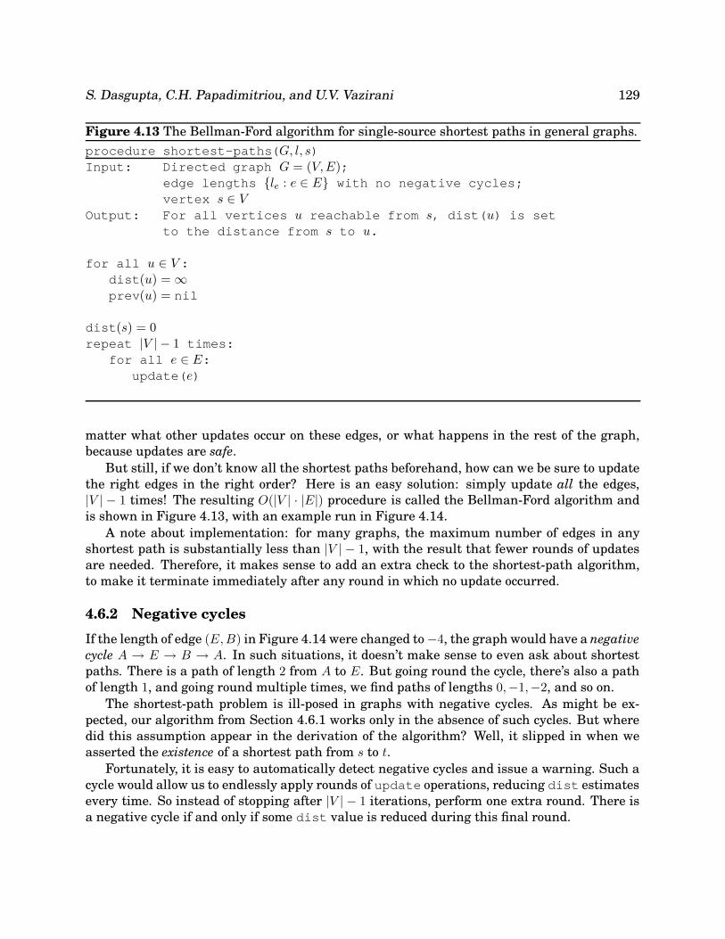
Figure 4.13 The Bellman-Ford algorithm for single-source shortest paths in general graphs.procedure shortest-paths(G, l, s)Input: Directed graph G = (V,E);

edge lengths le : e ∈ E with no negative cycles;vertex s ∈ V

Output: For all vertices u reachable from s, dist(u) is setto the distance from s to u.


dist(s) = 0repeat |V | − 1 times:

for all e ∈ E:update(e)

matter what other updates occur on these edges, or what happens in the rest of the graph,because updates are safe.

But still, if we don’t know all the shortest paths beforehand, how can we be sure to updatethe right edges in the right order? Here is an easy solution: simply update all the edges,|V | − 1 times! The resulting O(|V | · |E|) procedure is called the Bellman-Ford algorithm andis shown in Figure 4.13, with an example run in Figure 4.14.

A note about implementation: for many graphs, the maximum number of edges in anyshortest path is substantially less than |V | − 1, with the result that fewer rounds of updatesare needed. Therefore, it makes sense to add an extra check to the shortest-path algorithm,to make it terminate immediately after any round in which no update occurred.

4.6.2 Negative cyclesIf the length of edge (E,B) in Figure 4.14 were changed to−4, the graph would have a negativecycle A → E → B → A. In such situations, it doesn’t make sense to even ask about shortestpaths. There is a path of length 2 from A to E. But going round the cycle, there’s also a pathof length 1, and going round multiple times, we find paths of lengths 0,−1,−2, and so on.

The shortest-path problem is ill-posed in graphs with negative cycles. As might be ex-pected, our algorithm from Section 4.6.1 works only in the absence of such cycles. But wheredid this assumption appear in the derivation of the algorithm? Well, it slipped in when weasserted the existence of a shortest path from s to t.

Fortunately, it is easy to automatically detect negative cycles and issue a warning. Such acycle would allow us to endlessly apply rounds of update operations, reducing dist estimatesevery time. So instead of stopping after |V | − 1 iterations, perform one extra round. There isa negative cycle if and only if some dist value is reduced during this final round.

130 Algorithms

Figure 4.14 The Bellman-Ford algorithm illustrated on a sample graph.

E

B

A

G

F

D

S

C

3

1

1

−2

2

10

−1

−1

−4

1

8 IterationNode 0 1 2 3 4 5 6 7

S 0 0 0 0 0 0 0 0A ∞ 10 10 5 5 5 5 5B ∞ ∞ ∞ 10 6 5 5 5C ∞ ∞ ∞ ∞ 11 7 6 6D ∞ ∞ ∞ ∞ ∞ 14 10 9E ∞ ∞ 12 8 7 7 7 7F ∞ ∞ 9 9 9 9 9 9G ∞ 8 8 8 8 8 8 8

4.7 Shortest paths in dagsThere are two subclasses of graphs that automatically exclude the possibility of negative cy-cles: graphs without negative edges, and graphs without cycles. We already know how toefficiently handle the former. We will now see how the single-source shortest-path problemcan be solved in just linear time on directed acyclic graphs.

As before, we need to perform a sequence of updates that includes every shortest path asa subsequence. The key source of efficiency is that

In any path of a dag, the vertices appear in increasing linearized order.

Therefore, it is enough to linearize (that is, topologically sort) the dag by depth-first search,and then visit the vertices in sorted order, updating the edges out of each. The algorithm isgiven in Figure 4.15.

Notice that our scheme doesn’t require edges to be positive. In particular, we can findlongest paths in a dag by the same algorithm: just negate all edge lengths.


Figure 4.15 A single-source shortest-path algorithm for directed acyclic graphs.procedure dag-shortest-paths(G, l, s)Input: Dag G = (V,E);

edge lengths le : e ∈ E; vertex s ∈ VOutput: For all vertices u reachable from s, dist(u) is set



dist(s) = 0Linearize Gfor each u ∈ V , in linearized order:

for all edges (u, v) ∈ E:update(u, v)

132 Algorithms

Exercises4.1. Suppose Dijkstra’s algorithm is run on the following graph, starting at node A.

A B C D

E F G H

1 2

41268

5

64

1 1

1

(a) Draw a table showing the intermediate distance values of all the nodes at each iteration ofthe algorithm.

(b) Show the final shortest-path tree.

4.2. Just like the previous problem, but this time with the Bellman-Ford algorithm.

B

G H

I

C D

F

E

S

A

7

1

−4

6

5

3

−2

3

2−2

6

4

−2

1

−1 1

4.3. Squares. Design and analyze an algorithm that takes as input an undirected graph G = (V,E)and determines whether G contains a simple cycle (that is, a cycle which doesn’t intersect itself)of length four. Its running time should be at most O(|V |3).You may assume that the input graph is represented either as an adjacency matrix or withadjacency lists, whichever makes your algorithm simpler.

4.4. Here’s a proposal for how to find the length of the shortest cycle in an undirected graph with unitedge lengths.

When a back edge, say (v, w), is encountered during a depth-first search, it forms acycle with the tree edges from w to v. The length of the cycle is level[v]− level[w] + 1,where the level of a vertex is its distance in the DFS tree from the root vertex. Thissuggests the following algorithm:• Do a depth-first search, keeping track of the level of each vertex.• Each time a back edge is encountered, compute the cycle length and save it if it is

smaller than the shortest one previously seen.

Show that this strategy does not always work by providing a counterexample as well as a brief(one or two sentence) explanation.


4.5. Often there are multiple shortest paths between two nodes of a graph. Give a linear-time algo-rithm for the following task.

Input: Undirected graph G = (V,E) with unit edge lengths; nodes u, v ∈ V .Output: The number of distinct shortest paths from u to v.

4.6. Prove that for the array prev computed by Dijkstra’s algorithm, the edges u,prev[u] (for allu ∈ V ) form a tree.

4.7. You are given a directed graph G = (V,E) with (possibly negative) weighted edges, along with aspecific node s ∈ V and a tree T = (V,E ′), E′ ⊆ E. Give an algorithm that checks whether T is ashortest-path tree for G with starting point s. Your algorithm should run in linear time.

4.8. Professor F. Lake suggests the following algorithm for finding the shortest path from node s tonode t in a directed graph with some negative edges: add a large constant to each edge weight sothat all the weights become positive, then run Dijkstra’s algorithm starting at node s, and returnthe shortest path found to node t.Is this a valid method? Either prove that it works correctly, or give a counterexample.

4.9. Consider a directed graph in which the only negative edges are those that leave s; all other edgesare positive. Can Dijkstra’s algorithm, started at s, fail on such a graph? Prove your answer.

4.10. You are given a directed graph with (possibly negative) weighted edges, in which the shortestpath between any two vertices is guaranteed to have at most k edges. Give an algorithm thatfinds the shortest path between two vertices u and v in O(k|E|) time.

4.11. Give an algorithm that takes as input a directed graph with positive edge lengths, and returnsthe length of the shortest cycle in the graph (if the graph is acyclic, it should say so). Youralgorithm should take time at most O(|V |3).

4.12. Give an O(|V |2) algorithm for the following task.

Input: An undirected graph G = (V,E); edge lengths le > 0; an edge e ∈ E.Output: The length of the shortest cycle containing edge e.

4.13. You are given a set of cities, along with the pattern of highways between them, in the form of anundirected graph G = (V,E). Each stretch of highway e ∈ E connects two of the cities, and youknow its length in miles, le. You want to get from city s to city t. There’s one problem: your carcan only hold enough gas to cover L miles. There are gas stations in each city, but not betweencities. Therefore, you can only take a route if every one of its edges has length le ≤ L.

(a) Given the limitation on your car’s fuel tank capacity, show how to determine in linear timewhether there is a feasible route from s to t.

(b) You are now planning to buy a new car, and you want to know the minimum fuel tankcapacity that is needed to travel from s to t. Give an O((|V | + |E|) log |V |) algorithm todetermine this.

4.14. You are given a strongly connected directed graph G = (V,E) with positive edge weights alongwith a particular node v0 ∈ V . Give an efficient algorithm for finding shortest paths between allpairs of nodes, with the one restriction that these paths must all pass through v0.

4.15. Shortest paths are not always unique: sometimes there are two or more different paths with theminimum possible length. Show how to solve the following problem in O((|V |+ |E|) log |V |) time.

134 Algorithms

Input: An undirected graph G = (V,E); edge lengths le > 0; starting vertex s ∈ V .Output: A Boolean array usp[·]: for each node u, the entry usp[u] should be true ifand only if there is a unique shortest path from s to u. (Note: usp[s] = true.)


Figure 4.16 Operations on a binary heap.procedure insert(h, x)bubbleup(h, x, |h|+ 1)

procedure decreasekey(h, x)bubbleup(h, x, h−1(x))

function deletemin(h)if |h| = 0:

return nullelse:

x = h(1)siftdown(h, h(|h|), 1)return x

function makeheap(S)h = empty array of size |S|for x ∈ S:

h(|h|+ 1) = xfor i = |S| downto 1:

siftdown(h, h(i), i)return h

procedure bubbleup(h, x, i)(place element x in position i of h, and let it bubble up)p = di/2ewhile i 6= 1 and key(h(p)) > key(x):

h(i) = h(p); i = p; p = di/2eh(i) = x

procedure siftdown(h, x, i)(place element x in position i of h, and let it sift down)c = minchild(h, i)while c 6= 0 and key(h(c)) < key(x):

h(i) = h(c); i = c; c = minchild(h, i)h(i) = x

function minchild(h, i)(return the index of the smallest child of h(i))if 2i > |h|:

return 0 (no children)else:

return arg minkey(h(j)) : 2i ≤ j ≤ min|h|, 2i + 1

136 Algorithms

4.16. Section 4.5.2 describes a way of storing a complete binary tree of n nodes in an array indexed by1, 2, . . . , n.

(a) Consider the node at position j of the array. Show that its parent is at position bj/2c andits children are at 2j and 2j + 1 (if these numbers are ≤ n).

(b) What the corresponding indices when a complete d-ary tree is stored in an array?

Figure 4.16 shows pseudocode for a binary heap, modeled on an exposition by R.E. Tarjan.2 Theheap is stored as an array h, which is assumed to support two constant-time operations:

• |h|, which returns the number of elements currently in the array;• h−1, which returns the position of an element within the array.

The latter can always be achieved by maintaining the values of h−1 as an auxiliary array.

(c) Show that the makeheap procedure takes O(n) time when called on a set of n elements.What is the worst-case input? (Hint: Start by showing that the running time is at most∑n

i=1 log(n/i).)(a) What needs to be changed to adapt this pseudocode to d-ary heaps?

4.17. Suppose we want to run Dijkstra’s algorithm on a graph whose edge weights are integers in therange 0, 1, . . . ,W , where W is a relatively small number.

(a) Show how Dijkstra’s algorithm can be made to run in time O(W |V |+ |E|).(b) Show an alternative implementation that takes time just O((|V |+ |E|) logW ).

4.18. In cases where there are several different shortest paths between two nodes (and edges havevarying lengths), the most convenient of these paths is often the one with fewest edges. Forinstance, if nodes represent cities and edge lengths represent costs of flying between cities, theremight be many ways to get from city s to city twhich all have the same cost. The most convenientof these alternatives is the one which involves the fewest stopovers. Accordingly, for a specificstarting node s, define

best[u] = minimum number of edges in a shortest path from s to u.

In the example below, the best values for nodes S,A,B,C,D,E, F are 0, 1, 1, 1, 2, 2, 3, respectively.

S

A

B

C

D

E

F

2

24 3

2

2 1

1

1

1

Give an efficient algorithm for the following problem.

Input: Graph G = (V,E); positive edge lengths le; starting node s ∈ V .Output: The values of best[u] should be set for all nodes u ∈ V .

2See: R. E. Tarjan, Data Structures and Network Algorithms, Society for Industrial and Applied Mathematics,1983.


4.19. Generalized shortest-paths problem. In Internet routing, there are delays on lines but also, moresignificantly, delays at routers. This motivates a generalized shortest-paths problem.Suppose that in addition to having edge lengths le : e ∈ E, a graph also has vertex costscv : v ∈ V . Now define the cost of a path to be the sum of its edge lengths, plus the costs ofall vertices on the path (including the endpoints). Give an efficient algorithm for the followingproblem.

Input: A directed graph G = (V,E); positive edge lengths le and positive vertex costscv ; a starting vertex s ∈ V .Output: An array cost[·] such that for every vertex u, cost[u] is the least cost of anypath from s to u (i.e., the cost of the cheapest path), under the definition above.

Notice that cost[s] = cs.

4.20. There is a network of roads G = (V,E) connecting a set of cities V . Each road in E has anassociated length le. There is a proposal to add one new road to this network, and there is a listE′ of pairs of cities between which the new road can be built. Each such potential road e′ ∈ E′ hasan associated length. As a designer for the public works department you are asked to determinethe road e′ ∈ E′ whose addition to the existing networkG would result in the maximum decreasein the driving distance between two fixed cities s and t in the network. Give an efficient algorithmfor solving this problem.

4.21. Shortest path algorithms can be applied in currency trading. Let c1, c2, . . . , cn be various cur-rencies; for instance, c1 might be dollars, c2 pounds, and c3 lire. For any two currencies ci andcj , there is an exchange rate ri,j ; this means that you can purchase ri,j units of currency cj inexchange for one unit of ci. These exchange rates satisfy the condition that ri,j · rj,i < 1, so that ifyou start with a unit of currency ci, change it into currency cj and then convert back to currencyci, you end up with less than one unit of currency ci (the difference is the cost of the transaction).

(a) Give an efficient algorithm for the following problem: Given a set of exchange rates ri,j ,and two currencies s and t, find the most advantageous sequence of currency exchanges forconverting currency s into currency t. Toward this goal, you should represent the currenciesand rates by a graph whose edge lengths are real numbers.

The exchange rates are updated frequently, reflecting the demand and supply of the variouscurrencies. Occasionally the exchange rates satisfy the following property: there is a sequence ofcurrencies ci1 , ci2 , . . . , cik

such that ri1,i2 · ri2,i3 · · · rik−1 ,ik· rik ,i1 > 1. This means that by starting

with a unit of currency ci1 and then successively converting it to currencies ci2 , ci3 , . . . , cik, and

finally back to ci1 , you would end up with more than one unit of currency ci1 . Such anomalieslast only a fraction of a minute on the currency exchange, but they provide an opportunity forrisk-free profits.

(b) Give an efficient algorithm for detecting the presence of such an anomaly. Use the graphrepresentation you found above.

4.22. The tramp steamer problem. You are the owner of a steamship that can ply between a groupof port cities V . You make money at each port: a visit to city i earns you a profit of pi dollars.Meanwhile, the transportation cost from port i to port j is cij > 0. You want to find a cyclic routein which the ratio of profit to cost is maximized.

138 Algorithms

To this end, consider a directed graph G = (V,E) whose nodes are ports, and which has edgesbetween each pair of ports. For any cycle C in this graph, the profit-to-cost ratio is

r(C) =

∑(i,j)∈C pj∑(i,j)∈C cij

.

Let r∗ be the maximum ratio achievable by a simple cycle. One way to determine r∗ is by binarysearch: by first guessing some ratio r, and then testing whether it is too large or too small.Consider any positive r > 0. Give each edge (i, j) a weight of wij = rcij − pj .

(a) Show that if there is a cycle of negative weight, then r < r∗.(b) Show that if all cycles in the graph have strictly positive weight, then r > r∗.(c) Give an efficient algorithm that takes as input a desired accuracy ε > 0 and returns a simple

cycle C for which r(C) ≥ r∗ − ε. Justify the correctness of your algorithm and analyze itsrunning time in terms of |V |, ε, and R = max(i,j)∈E(pj/cij).

paths in graphs - university of california, berkeleyvazirani/algorithms/... · · 2006-10-03this...

Documents