Chaos, Solitons & Fractals 57 (2013) 129–136

Contents lists available at ScienceDirect

Chaos, Solitons & FractalsNonlinear Science, and Nonequilibrium and Complex Phenomena

journal homepage: www.elsevier .com/locate /chaos

Path probability distribution of stochastic motion of nondissipative systems: a classical analog of Feynman factorof path integral

0960-0779/$ - see front matter � 2013 Elsevier Ltd. All rights reserved.http://dx.doi.org/10.1016/j.chaos.2013.10.002

⇑ Corresponding author at: LUNAM Université, ISMANS, Laboratoire dePhysique Statistique et Systèmes Complexes, 44, Avenue F.A. Bartholdi, LeMans, France.

E-mail address: awang@ismans.fr (Q.A. Wang).

T.L. Lin a,b,c, R. Wang d, W.P. Bi b, A. El Kaabouchi a, C. Pujos a, F. Calvayrac b, Q.A. Wang a,b,⇑a LUNAM Université, ISMANS, Laboratoire de Physique Statistique et Systèmes Complexes, 44, Avenue F.A. Bartholdi, Le Mans, Franceb Faculté des Sciences et Techniques, Université du Maine, Ave. O. Messiaen, 72035 Le Mans, Francec Department of Physics, Xiamen University, Xiamen 361005, Chinad College of Information Science and Engineering, Huajiao University, Quanzhou 362021, China

a r t i c l e i n f o

Article history:Received 22 January 2013Accepted 2 October 2013Available online 31 October 2013

a b s t r a c t

We investigate, by numerical simulation, the path probability of non dissipative mechan-ical systems undergoing stochastic motion. The aim is to search for the relationshipbetween this probability and the usual mechanical action. The model of simulation is aone-dimensional particle subject to conservative force and Gaussian random displacement.The probability that a sample path between two fixed points is taken is computed from thenumber of particles moving along this path, an output of the simulation, divided by thetotal number of particles arriving at the final point. It is found that the path probabilitydecays exponentially with increasing action of the sample paths. The decay rate increaseswith decreasing randomness. This result supports the existence of a classical analog of theFeynman factor in the path integral formulation of quantum mechanics for Hamiltoniansystems.

� 2013 Elsevier Ltd. All rights reserved.

1. Introduction

The path (trajectory) of stochastic dynamics in mechan-ics has much richer physics content than that of the regularor deterministic motion. A path of regular motion alwayshas probability one once it is determined by the equationof motion and the boundary conditions, while a random mo-tion may have many possible paths under the same condi-tions, as can be easily verified with any stochastic process[1]. For a given process between two given states (or config-uration points with given durations), each of those potentialpaths has some chance (probability) to be followed. Thepath probability is a very important quantity for under-standing and characterizing random dynamics because it

contains all the information about the physics: the charac-teristics of the stochasticity, the degree of randomness, thedynamical uncertainty, the equations of motion and soforth. Consideration of paths has long been regarded as apowerful approach to non equilibrium thermodynamics[2–14]. A key question in this approach is what are the ran-dom variables which determine the probability. The Onsager–Machlup type action [2,5–12] is one of the answers forGaussian irreversible process close to equilibrium wherethe path probability is an exponentially decreasing functionof the action calculated along thermodynamic paths in gen-eral [2]. This action has been extended to Cartesian space in[12]. The large deviation theory [3,4] suggests a rate func-tion to characterize an exponential path probability. Thereare other suggestions by the consideration of the energyalong the paths [13,14]. For a Markovian process withGaussian noises, the Wiener path measure [1] provides agood description of the path likelihood with the product ofGaussian distributions of the random variables.

130 T.L. Lin et al. / Chaos, Solitons & Fractals 57 (2013) 129–136

The question we want to answer in this work is the fol-lowing: suppose a mechanical random motion is trackable,i.e., the mechanical quantities of the motion under consid-eration such as position, velocity, mechanical energy andso on can be calculated with certain precision along thepaths, is it possible to use the time cumulation, along thepaths, of Hamiltonian or Lagrangian (action) to character-ize the path probability of that motion? Possible answershave been given in [13,14]. The author of [13] suggests thatthe path probability decreases exponentially with increas-ing average energy along the paths [13]. This theory risks aconflict with the regular mechanical motion in the limit ofvanishing randomness because the surviving path wouldbe the path of least average energy, while it is actuallythe path of least action. The proposition of [14] is a pathprobability decreasing exponentially with the sum of thesuccessive energy differences, which risks the similar con-flicts with regular mechanics mentioned above.

Another proposition, free from the above mentionedconflicts, is to relate the path probability to action, thekey quantity for determining paths of Hamiltonian systemsin classical mechanics. According to a theoretical work in[19–21], for the special case of Hamiltonian system con-serving statistically its energy, the path probability canbe distributed in exponential function e�cA of the actionA ¼

RðK � VÞdt where K is the kinetic energy, V the poten-

tial energy, c a characteristic parameter of the randomdynamics and the time integral is carried out along theconsidered path. This distribution function is analogousto the Feynman factor e

i�hA of quantum mechanics [15].

The Feynman factor is not a probability, but in the presenceof the quantum randomness, the action A indeed charac-terizes the way the system evolves along the configurationpaths from one quantum state to another [16]. In both(classical [19–21] and quantum [15]) versions, the systemstatistically remains Hamiltonian in spite of the classical orquantum randomness. The classical path is recoveredwhen the randomness is vanishing with infinite c or zeroPlanck constant �h.

The aim of this work is to check this prediction for clas-sical mechanics by means of numerical simulation of therandom motion of Hamiltonian systems. There are severalreasons for limiting this work to Hamiltonian systems.Firstly, action is only well defined for Hamiltonian (oftenenergy conservative) mechanical systems [17,18]. Sec-ondly, from the previous results [2–14] for diffusive andrandom motion (usually non conservative systems), thepaths do not simply depend on the usual action, in general.Thirdly, the random motion without dissipation is cer-tainly an ideal model, but it is also a good approximationto many real random motions which are weakly dampedwith negligible energy dissipation compared to the varia-tion of potential energy. These are the cases where the con-servative force is much larger than the friction ones. Inother words, the system is (statistically) governed by theconservative forces. These motions are frequently observedin Nature. We can imagine, e.g., a falling motion of a parti-cle which is sufficiently heavy to fall in a medium withacceleration approximately determined by the conserva-tive force during a limited time period, but not too heavyin order to undergo observable randomness due to the

collision from the molecules around it or to other sourcesof randomness. Other examples include the frequently usedideal models of thermodynamic processes, such as the freeexpansion of isolated ideal gas and the heat conductionwithin perfectly isolated systems which, in spite of thethermal fluctuation, statistically conserve energy duringthe motion. Hence the result of this work is expected notonly to answer a fundamental question concerning pathprobability and action, but also to be useful as a mathemat-ical tool for investigating some real dynamics.

This ideal model can be depicted as the followingLangevin equation

md2x

dt2 ¼ �dVðxÞ

dx�mf

dxdtþ R; ð1Þ

with the zero friction limit (friction coefficient f! 0),where x is the one dimensional position, t the time, VðxÞthe potential energy and R the Gaussian distributed ran-dom force. For this motion, a stochastic Hamiltonian/Lagrangian mechanics has been formulated in [19–21]where a path entropy is introduced to measure the dynam-ical randomness or uncertainty in the path probability dis-tribution. When this path entropy takes the form of theShannon formula, the maximum entropy calculus stem-ming from an stochastic version of least action principleleads to an exponentially decreasing path probability withincreasing action. The numerical simulation of this work toverify this theoretical prediction can be summarized as fol-lows. We track the motion of a large number of particlessubject to a conservative force and a Gaussian distributedrandom displacement. The number of particles from onegiven position to another through some sample paths iscounted. When the total number of particles are suffi-ciently large, the probability (or its density) of a given pathis calculated by dividing the number of particles countedalong this path by the total number of particles arrivingat the end point through all the sample paths. The correla-tion of this probability distribution with two mechanicalquantities, the action and the time integral of Hamiltoniancalculated along the sample paths, is analyzed. In whatfollows, we first give a detailed description of thesimulation, followed by the analysis of the results andthe conclusion.

2. Technical details of numerical computation

The numerical model of the random motion can be out-lined as follows. The particles are subject to a conservativeforce and a Gaussian noise (random displacements v, seeEq. (3) below) and move along the axis x from an initialpoint a (position x0) to a final point b (xn) over a given per-iod of time ndt where n is the total number of discretesteps and dt ¼ ti � ti�1 the time increment of a step whichis the same for every step. Many different paths are possi-ble, each one being a sequence of random positionsfx0; x1; x2 . . . xn�1; xng, where xi is the position at time ti

(i ¼ 0;1;2 . . . n) and generated from a discrete time solu-tion of Eq. (1):

xi ¼ xi�1 þ vi þ f ðtiÞ � f ðti�1Þ; ð2Þ

0 0.2 0.4 0.6 0.8 1x 10−4

−2

−1.5

−1

−0.5

0

0.5

1

1.5x 10−8

Time (s)

Posi

tion

(m)

b

a

0 0.2 0.4 0.6 0.8 1 1.2 1.4x 10−26

10−8

10−7

10−6

10−5

10−4

10−3

Action (Js)

ln P

(A)

Fig. 1. Result for free particles. The left panel shows the axial lines of the sample paths between the given points a and b. The right panel shows the pathprobability distribution against the Lagrangian and Hamiltonian actions which are equal here as VðxÞ ¼ 0. The straight line is a best fit of the points with aslope of about �6:7� 1026 J�1 s�1.

T.L. Lin et al. / Chaos, Solitons & Fractals 57 (2013) 129–136 131

which is a superposition of a Gaussian random displace-ment vi and a regular motion yi ¼ f ðtiÞ, the solution of

the Newtonian equation m d2xdt2 ¼ � dVðxÞ

dx corresponding to

the least action path. Naturally, Eq. (2) is a solution of Eq.(1) under the condition that the superposition principleis valid for this motion. This principle should work when-ever Eq. (1) is linear, for instance, without force, or withconstant and harmonic forces. The reader will find thatwe have also used two others forces which make Eq. (1)nonlinear and may invalidate the superposition propertyof Eq. (2). Nevertheless linear equation is sufficient butnot necessary for superposition. From the fact that the re-sults from these two potentials are similar to those fromlinear equation, the superposition seems to work, at leastapproximately. We think that this positive result with non-linear forces may be attributed to two favorable elements:(1) most of the random displacements per step are smallcompared to the regular displacement; (2) the random nat-ure of these small displacements may statistically cancelthe nonlinear deviation from superposition property.

For each simulation, we select about 100 sample pathsrandomly created around the least action path y ¼ f ðtÞ.The magnitude of the Gaussian random displacements iscontrolled to ensure that all the sample paths are suffi-ciently smooth but sufficiently different from each otherto give distinct values of action and energy integral.

A width d is given to each sample path which becomes asmooth tube with the axial line composed of a sequence ofpositions fz0; z1; z2 . . . zn�1; zng. The reason for this is the fol-lowing. In principle, the probability of a single path (a geo-metrical line fx0; x1; x2 . . . xn�1; xng with zero thickness) isvanishingly small. Only its probability density is meaning-ful, as discussed later in the conclusion. We should specifyhere that, in practice, with the limited number of particlesin a simulation and the precision of the position, there arehardly more than one particle moving along a same geo-metrical line fx0; x1; x2 . . . xn�1; xng. Typically we have oneparticle along one geometrical line saved in the output ofthe simulation.

To calculate the probability density, a sample path mustbe defined as a tube of finite thickness d (a band in the x� t

representation). As all the particles or their trajectoriesfrom a to b are saved in the simulation, the number Nk ofparticles (or geometrical lines) going through a given sam-ple path or tube k, i.e., all the sequences of positionsfx0; x1; x2 . . . xn�1; xng satisfying fzigk � d=2 6 xi 6 fzigkþd=2 for all i ¼ 1;2 . . . n, can be counted, fz0; z1; z2 . . .

zn�1; zngk being the axial line of that tube. The probabilitythat the path k is taken is given by Pk ¼ Nk=N where N isthe total number of particles (trajectories) moving from ato b through all the considered sample paths. Pk for eachsample path fluctuates a lot from one simulation to an-other when the total number of particles simulated issmall, and tends to a stable value when we gradually in-crease the particle number. The largest number of particleswe used is 109 at which the value of Pk for a given samplepath does not change significantly even the number of par-ticles is increased further.

The probability density qk of the sample path k is de-fined by qk ¼

pkdn for a path of n steps. In this paper, the value

of Pk is used everywhere for the sake of simplicity.Some words about the thickness d of the sample paths. d

must be sufficiently large in order to include a considerablenumber of trajectories in each tube for the calculation ofreliable path probability, but sufficiently small in orderthat the positions zi and the instantaneous velocities v i

determined along an axial line be representative of allthe trajectories in a tube. If d is too small, there will befew particles going through each tube, making the calcu-lated probability too uncertain. If it is too large, zi and v i,as well as the energy and action of the axial line will notbe enough representative of all the trajectories in the tube.The d used in this work is chosen to be 1/2 of the standarddeviation r of the Gaussian distribution of random dis-placements. The left panels of Figs. 1–5 illustrate the axiallines of the sample paths.

For each sample path, the instantaneous velocity at thestep i is calculated by v i ¼ zi�zi�1

ti�ti�1along the axial line. This

velocity can be approximately considered as the averagevelocity of all the trajectories passing through the tube.The kinetic energy is given by Ki ¼ 1

2 mv2i , the action by

AL ¼P10

i¼1½12 mv2i � VðxiÞ� � dt, called Langrangian action

0 0.2 0.4 0.6 0.8 1x 10−4

−3

−2.5

−2

−1.5

−1

−0.5

0

0.5

1x 10−8

Time (s)

Posi

tion

(m)

a

b

−0.5 0 0.5 1 1.5 2 2.5x 10−26

10−8

10−7

10−6

10−5

10−4

10−3

Action (Js)

ln P

(A)

Lagrangian ActionHamiltonian Action

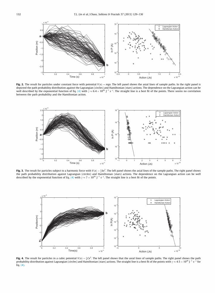
Fig. 2. The result for particles under constant force with potential VðxÞ ¼ mgx. The left panel shows the axial lines of sample paths. In the right panel isdepicted the path probability distribution against the Lagrangian (circles) and Hamiltonian (stars) actions. The dependence on the Lagrangian action can bewell described by the exponential function of Eq. (4) with c � 6:4� 1026 J�1 s�1. The straight line is a best fit of the points. There seems no correlationbetween the path probability and the Hamiltonian action.

0 0.2 0.4 0.6 0.8 1x 10−4

−2.5

−2

−1.5

−1

−0.5

0

0.5

1

1.5

2

2.5x 10−8

Time (s)

Posi

tion

(m)

b

a

−1 0 1 2 3 4 5 6 7x 10−26

10−8

10−7

10−6

10−5

10−4

Action (Js)

ln P

(A)Lagrangian ActionHamiltonian Action

Fig. 3. The result for particles subject to a harmonic force with VðxÞ ¼ 12 kx2. The left panel shows the axial lines of the sample paths. The right panel shows

the path probability distribution against Lagrangian (circles) and Hamiltonian (stars) actions. The dependence on the Lagrangian action can be welldescribed by the exponential function of Eq. (4) with c � 7� 1026 J�1 s�1. The straight line is a best fit of the points.

0 0.2 0.4 0.6 0.8 1x 10−4

−5

−4

−3

−2

−1

0

1

2x 10−8

Time(s)

Posi

tion(

m)

b

a

−5 0 5 10x 10−26

10−8

10−7

10−6

10−5

10−4

10−3

10−2

Action (Js)

ln P

(A)

Lagrangian ActionHamiltonian Action

Fig. 4. The result for particles in a cubic potential VðxÞ ¼ 13 Cx3. The left panel shows that the axial lines of sample paths. The right panel shows the path

probability distribution against Lagrangian (circles) and Hamiltonian (stars) actions. The straight line is a best fit of the points with c � 4:5� 1026 J�1 s�1 forEq. (4).

132 T.L. Lin et al. / Chaos, Solitons & Fractals 57 (2013) 129–136

0 0.2 0.4 0.6 0.8 1x 10−4

−0.5

0

0.5

1

1.5

2

2.5

3x 10−8

Time (s)

Posi

tion

(m)

a

b

0 0.5 1 1.5x 10−26

10−8

10−7

10−6

10−5

10−4

Action (Js)

ln P

(A)

Lagrangian ActionHamiltonian Action

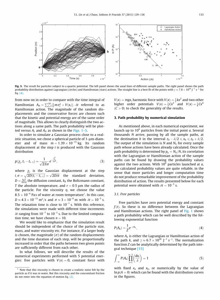
Fig. 5. The result for particles subject to a quartic potential. The left panel shows the axial lines of different sample paths. The right panel shows the pathprobability distribution against Lagrangian (circles) and Hamiltonian (stars) actions. The straight line is a best fit of the points with c � 7:8� 1026 J�1 s�1 forEq. (4).

T.L. Lin et al. / Chaos, Solitons & Fractals 57 (2013) 129–136 133

from now on in order to compare with the time integral of

Hamiltonian AH ¼P10

i¼1½12 mv2i þ VðxiÞ� � dt referred to as

Hamiltonian action. The magnitude of the random dis-placements and the conservative forces are chosen suchthat the kinetic and potential energy are of the same orderof magnitude. This allows to clearly distinguish the two ac-tions along a same path. The path probability will be plot-ted versus AL and AH as shown in the Figs. 1–5.

In order to simulate a Gaussian process close to a real-istic situation, we chose a spherical particle of 1-lm-diam-eter and of mass m ¼ 1:39� 10�15 kg. Its randomdisplacement at the step i is produced with the Gaussiandistribution

pðvi; ti � ti�1Þ ¼1ffiffiffiffiffiffiffi

2pp

re�

v2i

2r2 ; ð3Þ

where vi is the Gaussian displacement at the stepi;r ¼

ffiffiffiffiffiffiffiffiffiffiffiffiffiffiffiffiffiffiffiffiffiffiffiffiffiffi2Dðti � ti�1Þ

p¼

ffiffiffiffiffiffiffiffiffiffiffi2Ddtp

the standard deviation,

D ¼ kBT6prg the diffusion constant, kB the Boltzmann constant,

T the absolute temperature, and r ¼ 0:5 lm the radius ofthe particle. For the viscosity g, we choose the value8:5� 10�4 Pas of water at room temperature1. In this case,D � 4:3� 10�13 m2=s and r � 3� 10�9 m with dt ¼ 10�5 s.The relaxation time is close to 10�7 s. With this reference,the simulations were made with different time incrementsdt ranging from 10�7 to 10�3 s. Due to the limited computa-tion time, we have chosen n ¼ 10.

We would like to emphasize that the simulation resultshould be independent of the choice of the particle size,mass, and water viscosity etc. For instance, if a larger bodyis chosen, the magnitude (r) of the random displacementsand the time duration of each step, will be proportionallyincreased in order that the paths between two given pointsare sufficiently different from each other.

In what follows, we will describe the results of thenumerical experiments performed with 5 potential ener-gies: free particles with VðxÞ ¼ 0, constant force with

1 Note that this viscosity is chosen to create a realistic noise felt by theparticle as if it was in water. But this viscosity and the concomitant frictiondo not enter into the equation of motion Eq. (2).

VðxÞ ¼ mgx, harmonic force with VðxÞ ¼ 12 kx2 and two other

higher order potentials VðxÞ ¼ 13 Cx3 and VðxÞ ¼ 1

4 Cx4

ðC > 0Þ to check the generality of the results.

3. Path probability by numerical simulation

As mentioned above, in each numerical experiment, welaunch up to 109 particles from the initial point a. Severalthousands N arrive, passing by all the sample paths, atthe destination b in the interval zb � d=2 6 xb 6 zb þ d=2.The output of the simulation is N and Nk for every samplepath whose actions have been already calculated. Once thepath probability is determined by pk ¼ Nk=N, its correlationwith the Lagrangian or Hamiltonian action of the samplepaths can be found by drawing the probability valuesagainst the two actions. With 109 particles launched at a,the calculated probability values are quite reliable, in thesense that more particles and longer computation timedo not produce remarkable improvement of the probabilitydistribution of action. The results presented below for eachpotential were obtained with dt ¼ 10�5 s.

3.1. Free particles

Free particles have zero potential energy and constantf ðtÞ. So these is no difference between the Lagrangianand Hamiltonian actions. The right panel of Fig. 1 showsa path probability which can be well described by the fol-lowing exponential function

PðAkÞ ¼1Z

e�cAk ; ð4Þ

where Ak is either the Lagrangian or Hamiltonian action ofthe path k, and c � 6:7� 1026 J�1 s�1. The normalizationfunction Z can be analytically determined by the path inte-gral technique [15]Z 1

�1P Akð Þ

Yn�1

i¼1

dxi

d

� �¼ 1 ð5Þ

with fixed xa and xb, or numerically by the value ofln pðA ¼ 0Þwhich can be found with the distribution curvesin the figures.

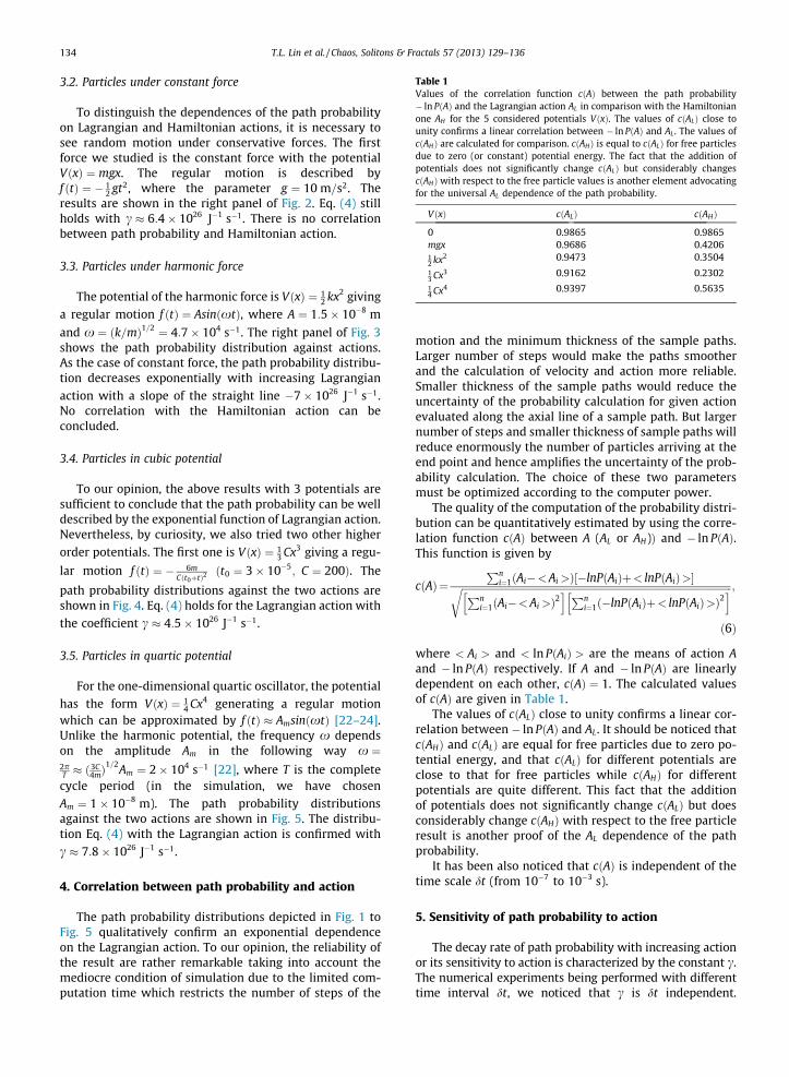
Table 1Values of the correlation function cðAÞ between the path probability� ln PðAÞ and the Lagrangian action AL in comparison with the Hamiltonianone AH for the 5 considered potentials VðxÞ. The values of cðALÞ close tounity confirms a linear correlation between � ln PðAÞ and AL . The values ofcðAHÞ are calculated for comparison. cðAHÞ is equal to cðALÞ for free particlesdue to zero (or constant) potential energy. The fact that the addition ofpotentials does not significantly change cðALÞ but considerably changescðAHÞ with respect to the free particle values is another element advocatingfor the universal AL dependence of the path probability.

VðxÞ cðALÞ cðAHÞ

0 0.9865 0.9865mgx 0.9686 0.420612 kx2 0.9473 0.3504

13 Cx3 0.9162 0.2302

14 Cx4 0.9397 0.5635

134 T.L. Lin et al. / Chaos, Solitons & Fractals 57 (2013) 129–136

3.2. Particles under constant force

To distinguish the dependences of the path probabilityon Lagrangian and Hamiltonian actions, it is necessary tosee random motion under conservative forces. The firstforce we studied is the constant force with the potentialVðxÞ ¼ mgx. The regular motion is described byf ðtÞ ¼ � 1

2 gt2, where the parameter g ¼ 10 m=s2. Theresults are shown in the right panel of Fig. 2. Eq. (4) stillholds with c � 6:4� 1026 J�1 s�1. There is no correlationbetween path probability and Hamiltonian action.

3.3. Particles under harmonic force

The potential of the harmonic force is VðxÞ ¼ 12 kx2 giving

a regular motion f ðtÞ ¼ AsinðxtÞ, where A ¼ 1:5� 10�8 m

and x ¼ ðk=mÞ1=2 ¼ 4:7� 104 s�1. The right panel of Fig. 3shows the path probability distribution against actions.As the case of constant force, the path probability distribu-tion decreases exponentially with increasing Lagrangianaction with a slope of the straight line �7� 1026 J�1 s�1.No correlation with the Hamiltonian action can beconcluded.

3.4. Particles in cubic potential

To our opinion, the above results with 3 potentials aresufficient to conclude that the path probability can be welldescribed by the exponential function of Lagrangian action.Nevertheless, by curiosity, we also tried two other higherorder potentials. The first one is VðxÞ ¼ 1

3 Cx3 giving a regu-

lar motion f ðtÞ ¼ � 6mCðt0þtÞ2

ðt0 ¼ 3� 10�5; C ¼ 200Þ. The

path probability distributions against the two actions areshown in Fig. 4. Eq. (4) holds for the Lagrangian action withthe coefficient c � 4:5� 1026 J�1 s�1.

3.5. Particles in quartic potential

For the one-dimensional quartic oscillator, the potentialhas the form VðxÞ ¼ 1

4 Cx4 generating a regular motionwhich can be approximated by f ðtÞ � AmsinðxtÞ [22–24].Unlike the harmonic potential, the frequency x dependson the amplitude Am in the following way x ¼2pT � ð3C

4mÞ1=2Am ¼ 2� 104 s�1 [22], where T is the complete

cycle period (in the simulation, we have chosenAm ¼ 1� 10�8 m). The path probability distributionsagainst the two actions are shown in Fig. 5. The distribu-tion Eq. (4) with the Lagrangian action is confirmed withc � 7:8� 1026 J�1 s�1.

4. Correlation between path probability and action

The path probability distributions depicted in Fig. 1 toFig. 5 qualitatively confirm an exponential dependenceon the Lagrangian action. To our opinion, the reliability ofthe result are rather remarkable taking into account themediocre condition of simulation due to the limited com-putation time which restricts the number of steps of the

motion and the minimum thickness of the sample paths.Larger number of steps would make the paths smootherand the calculation of velocity and action more reliable.Smaller thickness of the sample paths would reduce theuncertainty of the probability calculation for given actionevaluated along the axial line of a sample path. But largernumber of steps and smaller thickness of sample paths willreduce enormously the number of particles arriving at theend point and hence amplifies the uncertainty of the prob-ability calculation. The choice of these two parametersmust be optimized according to the computer power.

The quality of the computation of the probability distri-bution can be quantitatively estimated by using the corre-lation function cðAÞ between A (AL or AH)Þ and � ln PðAÞ.This function is given by

cðAÞ¼Pn

i¼1ðAi�<Ai >Þ½�lnPðAiÞþ< lnPðAiÞ>�ffiffiffiffiffiffiffiffiffiffiffiffiffiffiffiffiffiffiffiffiffiffiffiffiffiffiffiffiffiffiffiffiffiffiffiffiffiffiffiffiffiffiffiffiffiffiffiffiffiffiffiffiffiffiffiffiffiffiffiffiffiffiffiffiffiffiffiffiffiffiffiffiffiffiffiffiffiffiffiffiffiffiffiffiffiffiffiffiffiffiffiffiffiffiffiffiffiffiffiffiffiffiffiffiffiffiffiffiffiffiPni¼1ðAi�<Ai >Þ2

h i Pni¼1ð�lnPðAiÞþ< lnPðAiÞ>Þ2

h ir ;

ð6Þ

where < Ai > and < ln PðAiÞ > are the means of action Aand � ln PðAÞ respectively. If A and � ln PðAÞ are linearlydependent on each other, cðAÞ ¼ 1. The calculated valuesof cðAÞ are given in Table 1.

The values of cðALÞ close to unity confirms a linear cor-relation between � ln PðAÞ and AL. It should be noticed thatcðAHÞ and cðALÞ are equal for free particles due to zero po-tential energy, and that cðALÞ for different potentials areclose to that for free particles while cðAHÞ for differentpotentials are quite different. This fact that the additionof potentials does not significantly change cðALÞ but doesconsiderably change cðAHÞ with respect to the free particleresult is another proof of the AL dependence of the pathprobability.

It has been also noticed that cðAÞ is independent of thetime scale dt (from 10�7 to 10�3 s).

5. Sensitivity of path probability to action

The decay rate of path probability with increasing actionor its sensitivity to action is characterized by the constant c.The numerical experiments being performed with differenttime interval dt, we noticed that c is dt independent.

0 2 4 6 8 10 12x 1012

0

0.5

1

1.5

2

2.5

3

3.5

4x 1027

1/D (m−2s)

γ (J

−1s−1

)

Fig. 6. 1=D dependence of the decay rate c of path probability with action.The increase of c with increasing 1=D implies that the stochastic motion ismore dispersed around the least action path with more diffusivity. Theslope or the ratio c=ð1=DÞ is about 3:1� 1014 kg�1.

T.L. Lin et al. / Chaos, Solitons & Fractals 57 (2013) 129–136 135

Logically, this sensitivity should be dependent on the ran-domness of the Gaussian noise. Analysis of the probability dis-

tributions reveals that the ratio c=ð1=DÞ � 3:2� 1014 kg�1

for free particles, c=ð1=DÞ � 3:1� 1014 kg�1 for particles

subject to constant force, and c=ð1=DÞ � 1:7� 1014 kg�1

with harmonic force. Fig. 6. shows the 1=D dependence ofc for constant force as an example.

As expected, c increases with increasing 1=D, i.e., thestochastic motion is less dispersed around the least actionpath with decreasing diffusivity D. It is worth noticing thelinear 1=D dependence of c in the range studied here. Fromtheoretical point of view, c should tend to infinity for van-ishing D. This is the limit case of regular motion of Hamil-tonian mechanics. This asymptotic property can also beseen with the uncertainty relation of action given by thestandard deviation rA P 1ffiffi

2p

c[20]. To give an example,

when c ¼ 3� 1027 ðJsÞ�1; rA P 2:4� 10�28 Js. When c isinfinity, the least uncertainty of measure of action shouldbe zero, in principle.

6. Concluding remarks

To summarize, by numerical simulation of Gaussianstochastic motion of non dissipative systems, we haveshown the evidence of the exponential action dependenceof path probability. In spite of the uncertainty due to thelimited computation time, the computation of the mechan-ical quantities and the path probability is rigorous and reli-able. It is possible to improve the result by more precisecomputation with longer motion duration, thiner samplepaths and more particles. Experimental verification withweakly damped motion can also be expected.

Apart from the possibility of application to weaklydamped motion, the present result seems to provide, bythe striking similarity between classical stochastic motionand quantum motion of Hamiltonian systems concerningthe choice of paths, an opportunity for a deeper under-standing of random motions, and a new angle to see intothe random motions and their relationship with non

equilibrium statistical mechanics and thermodynamics, inbenefiting fully from the technique of path integral alreadydeveloped in quantum mechanics. An example of this toolborrowing is shown in [21] for the discussion of possibleclassical uncertainty relations.

Unlike the Feynman factor eiA=�h which is just a mathe-matical object, e�cA is a real function describing the pathprobability. This exponential form and the positivity of cimply that the most probable path is just the least actionpath of classical mechanics, and that when the noisediminishes, more and more paths will shrink into the bun-dle of least action paths. In the limit case of vanishingnoise, all paths collapse on the least action path, the mo-tion recovers the Newtonian dynamics.

The present result does not mean that the probabilityfor single trajectory necessarily exists. Each path consid-ered here is a tube of thickness d and is sufficiently smoothand thin for the instantaneous position and velocity deter-mined along its axial line to be representative for all thetrajectories in it. The probability of such a path should tendto zero when d! 0. However, the density of path probabil-ity should have a sense and can be defined byqk ¼ limd!0

Pkdn for any finite n, the number of steps of a dis-

crete random process.Again, we would like to stress that the present results

do not apply to the usual Brownian motion or similar over-damped stochastic motions. These motions have been wellstudied with Langevin, Fokker–Planck and Kolmogorovequations which include friction forces. This work is notat odds with these well established approaches. This is adifferent angle to address stochastic dynamics. It is ourhope that it will be applied to real stochastic dissipativemotion. This application needs, first of all, a fundamentalextension of the least action principle to dissipative regularmotion within classical mechanics. It is unimaginable thatthe action, being no more a characteristic variable of thepaths of regular motion, can come into play when the samemotion is perturbed by noise. This extension is anotherlong story, and has been the objective of unremitting ef-forts of physicists till now [17,18,25,26].

Acknowledgments

This work was supported by the Region des Pays de laLoire in France under the Grant No. 2007-6088 and No.2009-09333.

References

[1] Mazo RM. Brownian motion. Oxford University Press; 2002.[2] Onsager L, Machlup S. Phys Rev 1953;91:1505.[3] Freidlin MI, Wentzell AD. Random perturbation of dynamical

systems. New York: Springer-Verlag; 1984.[4] Touchette H. The large deviation approach to statistical mechanics.

Phys Rep 2009;478:1–69.[5] Maier RS, Stein DL. The escape problem for irreversible systems. Phys

Rev E 1993;48:931.[6] Aurell E, Sneppen K. Epigenetics as a first exit problem. Phys Rev Lett

2002;88:048101.[7] Roma DM, OFlanagan RA, Ruckenstein AE, Sengupta AM,

Mukhopadhyay R. Phys Rev E 2005;71:011902.[8] Cohen EGD. Properties of nonequilibrium steady states: a path

integral approach. J Stat Mech 2008:P07014.

136 T.L. Lin et al. / Chaos, Solitons & Fractals 57 (2013) 129–136

[9] Wang Jin, Zhang Kun, Wang Erkwang. Kinetic paths, time scale, andunderlying landscapes: a path integral framework to study globalnatures of nonequilibrium systems and networks. J Chem Phys2010;133:125103.

[10] Sadhukhan Poulomi, Bhattacharjee Somendra M. Thermodynamicsas a nonequilibrium path integral. J Phys A: Math Theor2010;43:245001.

[11] Stock Gerhard, Ghosh Kingshuk, Dill Ken A. Maximum caliber: avariational approach applied to two-state dynamics. J Chem Phys2008;128:194102.

[12] Fujisaki Hiroshi, Shiga Motoyuki, Kidera Akinori. Onsager–CMachlupaction-based path sampling and its combination with replicaexchange for diffusive and multiple pathways. J Chem Phys2010;132:134101.

[13] Evans RML. Detailed balance has a counterpart in non-equilibriumsteady states. J Phys A: Math Gen 2005;38:293 [cond-mat/0408614].

[14] Abaimov SG. General formalism of non-equilibrium statisticalmechanics a path approach, arXiv:0906.0190.

[15] Feynman RP, Hibbs AR. Quantum mechanics and path integrals. NewYork: McGraw-Hill Publishing Company; 1965.

[16] Pavon M. Stochastic mechanics and the Feynman integral. J MathPhys 2000;41:6060–78.

[17] Lanczos C. The variational principles of mechanics. New York: DoverPublication; 1986.

[18] Sieniutycz S, Farkas H. Variational and extremum principles inmacroscopic systems. Elsevier; 2005.

[19] Wang QA. Maximum path information and the principle of leastaction for chaotic system. Chaos Solitons Fract 2004;23:1253.

[20] Wang QA, Tsobnang F, Bangoup S, Dzangue F, Jeatsa A, Le Méhauté A,et al. Reformulation of a stochastic action principle for irregulardynamics. Chaos Solitons Fract 2009;40:2550 [arXiv:0704.0880].

[21] Wang QA. Non quantum uncertainty relations of stochasticdynamics. Chaos Solitons Fract 2005;26:1045 [arXiv:cond-mat/0412360].

[22] Gray CG, Taylor EF. When action is not least. Am J Phys2007;75:434–58.

[23] Gray CG, Karl G, Novikov VA. Progress in classical and quantumvariational principles. Rep Prog Phys 2004;67:159–208.

[24] Gray CG, Karl G, Novikov VA. Direct use of variational principles asan approximation technique in classical mechanics. Am J Phys1996;64:1177–84.

[25] Wang QA, Ru Wang. Is it possible to formulate least action principlefor dissipative systems? arXiv:1201.6309.

[26] Lin TL, Wang QA. The extrema of an action principle for dissipativemechanical systems. J Appl Mech 2013;81:031002.