path loss analysis of wsn wave propagation in vegetation
TRANSCRIPT

Journal of Physics Conference Series
OPEN ACCESS
Path Loss Analysis of WSN Wave Propagation inVegetationTo cite this article Naseer Sabri et al 2013 J Phys Conf Ser 423 012063
View the article online for updates and enhancements
You may also likeMeasuring Leaf Area in Soy Plants by HSIColor Model Filtering and MathematicalMorphologyM Benalcaacutezar J Padiacuten M Brun et al
-
Detecting spatiotemporal changes of peakfoliage coloration in deciduous andmixedforests across the Central andEastern United StatesLingling Liu Xiaoyang Zhang Yunyue Yuet al
-
Percentage Coverage of Tropical ClimbingPlants of Green FacadeMohd Khairul Azhar Mat Sulaiman MohdFairuz Shahidan Maslina Jamil et al
-
Recent citationsPath Loss Determination Using Linear andCubic Regression Inside a Classic TomatoGreenhouseDora Cama-Pinto et al
-
Link Investigation of IEEE 802154Wireless Sensor Networks in ForestsXingjian Ding et al
-
This content was downloaded from IP address 59137239130 on 12102021 at 1644
Path Loss Analysis of WSN Wave Propagation in Vegetation
Naseer Sabri1 S A Aljunid
1 M S Salim
2 R Kamaruddin
3 R B Ahmad
1 M F Malek
1 1 Computer and Communication Engineering School UniMAP Malaysia
2 Mechatronics Engineering School UniMAP Malaysia
3 Bioprocess Engineering School UniMAP Malaysia
E-mail nasseersabriyahoocom
Abstract Deployment of a successful wireless sensor network requires precise prediction
models that provide a reliable communication links of wireless nodes Prediction models fused
with foliage models provide sensible parameters of wireless nodes separation distance antenna
height and power transmission which affect the reliability and communication coverage of a
network This paper review the line of sight and the two ray propagation models combined
with the most known foliage models that cover the propagation of wireless communications in
vegetative environments using IEEE 802154 standard Simulation of models is presented and
the impacts of the communication parameters environment and vegetation have been reported
1 Introduction
Pervasive networks represented by wireless sensor actor network emerge the promises of automation
the environment with sensors-actors wireless nodes which yielding a new era of environment
automation applications [1] [2] Currently Wireless sensor network platform and applications are in
an exponential growing Initially they were oriented for indoor applications such as home automation
and industrial control or for medical applications such as elderly monitoring [3] Currently WSANs
are adopted in a wide range of applications including telemedicine home and building automation
surveillance systems and agricultural avoiding the expensive retrofit necessary in wired systems
WSN nodes are highly constrained in terms of physical size power consumption of CPU and
transceiver memory size and bandwidth For remote nodes the power consumption is considered a
crucial parameter and have to care precisely where energy efficiency is paramount and batteries may
have to last for years Indeed challenging physical environment like heat dust moisture rain and
interference [4]
WSN applications are growing exponentially and one of the most promising applications is the
precision agriculture Precision agriculture is one of the promising domains where wireless sensor
networks could be exploited for example by observing the micro-climate within a field so that
ultimately plant-specific farming can be realized Agricultural application relies on the use of new era
of WSAN to endorse monitoring and controlling management of a field based on site conditions [4]
WSNs offer a great flexibility when deploying new systems and when updating existing systems [5]
Since vegetation areas are cover a large portion of the Earthrsquos surface the propagation of radio waves
in a forest has long been of researcherrsquos interest Radio waves propagating in vegetation usually
experience much higher path loss than in environments without vegetation Therefore well known of
the propagation mechanisms through a forest is critical for communication and sensing in such
ScieTech 2013 IOP PublishingJournal of Physics Conference Series 423 (2013) 012063 doi1010881742-65964231012063
Published under licence by IOP Publishing Ltd 1
environments However WSN nodes are spatial distribution in the field and must consider all the
parameters that may have effects the wireless channel communication Currently the most promising
of WSN technology in agricultural field is ZigBee [6-8] This protocol has been widely adopted by
WSN developerrsquos community it relies on the IEEE 802154 standard [9] ZigBee technology is a low
rate low cost low power consumption wireless node protocol aiming to remote and automation
application systems
ZigBee is expected to provide low power and cost connectivity for nodes that need long operation of
battery of several years with low data rate The IEEE-ZigBee are expected to transmit over 10-75
meters based on the RF power output consumption for specific application and the environment and
operates in the unlicensed RF worldwide 24 GHz with 250 Kbps data rate To determine the
behaviour of electromagnetic waves a precise model of propagation must be adopted however
models normally used in wireless communication might not be precise describe the wireless sensor
network WSN node are spatially located usually near the earth surface thus may induce absence of
main ray between sender-receiver nodes which is known of no line of sight (NLOS) status occur
although WSN nodes have spatially short distance distribution Therefore WSN propagation waves
may face obstacle like trees fence building and dense foliage
2 Radio Wave Propagation
The wireless radio channel faces a severe challenge as a medium for reliable high speed
communication It is susceptible to interference noise and other channel impediments which may
change over time in unpredictable ways due to nodes-user movement Path loss is caused by
dissipation of the power radiated by the transmitter as well as effects of the propagation channel
Generally path loss models propose that path loss is same for a given distance between sources of
transmit and receive Shadowing is caused by obstacles between the transmitter and receiver which
will attenuate the signal power through reflection diffraction absorption and scattering For high
level of attenuation the signal will be blocked Variation due to path loss occurs over very large
distances (100-1000 meters) whereas variation due to shadowing occurs over distances proportional
to the length of the obstructing object (10-100 meters in outdoor environments and less in indoor
environments) [ 10 11] Such an environmental parameters not foreseen by developers and neither
considered by theoretical models and not accounted by simulators [11 12] are affecting the wireless
communication link This is especially true for an arable farming environment in which foliage
growing crops and ever changing weather conditions have an unknown effect on the exact
propagation of the radio waves The wireless channel is modelled based on several key parameters
These parameters vary significantly with the environment rural versus urban or flat versus
mountainous Different kinds of fading can be categorized in three types [13] [14]
Distance Dependence of path loss (measured in dB) is approximated by L (d) = L0 +10ntimeslog(d∕d0)
where n is the path loss exponent which varies with terrain and environment and L0 is the path loss at
an arbitrary reference distance d0
Large-scale Shadowing causes variations over larger areas and is caused by terrain building and
foliage obstructions the large-scale fading due to various obstacles is commonly accepted to follow a
log-normal distribution [15]) This means that its attenuation x measured in dB is normally distributed
N(m σ) with mean m and standard deviation σ The probability density function of x is given by the
usual Gaussian formula
Small-scale fading causes great variation within a half wavelength It is caused by multipath and
moving scatters Resulting fades are usually approximated by Rayleigh Rican or similar fading
statistics ndash measurements also show good fit to Nakagami-m and Weibull distributions
Radio systems rely on diversity equalizing channel coding and interleaving schemes to mitigate its
impact There are different propagation characteristic of different spectrum bands which require
different prediction models Some propagation models are well suited for computer simulation in
ScieTech 2013 IOP PublishingJournal of Physics Conference Series 423 (2013) 012063 doi1010881742-65964231012063
2
presence of detailed terrain and building data others aim at providing simpler general path loss
estimates [14 15] Wireless sensor network of mobile nodes are burdened with particular propagation
complications making reliable wireless communication more difficult than fixed communication
between and carefully positioned wireless nodes The antenna height at a mobile terminal is usually
very small typically less than a few meters Hence there is very little clearness so obstacles and
reflecting surfaces in the vicinity of the antenna have a substantial influence on the characteristics of
the propagation path Moreover the propagation characteristics change from place to place and if the
terminal moves from time to time
Path loss models define the attenuation of a signal as a function of the propagation distance between
a transmit and a receive antennas and other parameters Some models include many details of the
terrain profile to estimate the path loss while others just consider the signal frequency and the
separation distance Antenna heights are other critical parameters [13]
21 Free Space Propagation The free space propagation model assumes the influence of the earth surface to be entirely absent This model assumes that the transmitter and receiver antennas to be located in an otherwise empty environment Neither absorbing obstacles nor reflecting surfaces are considered [13][14] The radiated energy is spread over the surface of a sphere of radius d so as the propagation distance increases the power received decreases proportional to d
-2 The received power is
1020log ( ) (1)dB o oP P d d
Hence the free space propagation model assumes ideal propagation condition that there is only one clear line-of-sight path between the transmitter and receiver A physical argument of conservation of energy leads to the Friisrsquo power transmission formula in free space A transmitted power source Pt radiates spherically with an antenna gain Gt the power density W at distance d from a transmitter with power Pt and antenna gain Gt is
2 4 (2)T tW P G d
The portion of that power impinging an effective area Ae hence at a distance d the power is Pr=PtGtAe ∕ (4πd
2) The effective area of an antenna is related to antenna gain by Ae ∕ λ
2=Gt ∕4π which is used for
the receiving antenna and thus yields [13 14]
2( 4 ) (3)r t t rP PGG d
Pt Gt and Pr Gr are the transmitted and received power and gain respectively λ is the wavelength of the signal and d is the separation distance The product GtPt is called the effectively radiated power (ERP) of the transmitter The path loss reflects how much power is dissipated between transceiver and receiver antennas (without counting any antenna gain) Path loss is often expressed as a function of frequency (f) distance (d) and a scaling constant that contains all other factors of the formula Equation 3 shows a free-space dependence in 1∕d
2 and is sometimes loss is expressed in decibels (dB)
L(dB) = 10 times log(PTPr) For instance when fo = 1MHz and do = 1km the loss expressed as
10 10( ) 3244 20log ( ) 20log ( ) (4)o oL dB f f d d
The free space model basically represents the communication range as a circle around the transmitter If a receiver is within the circle it receives all packets Otherwise it loses all packets
22 Two-ray ground reflection model Ray tracing is a method that uses a geometric approach and examines what paths the wireless radio signal takes from transmitter to receiver as if each path was a ray of light (possibly reflecting off surfaces) Ray-tracing predictions are good when detailed information of the area is available But the
ScieTech 2013 IOP PublishingJournal of Physics Conference Series 423 (2013) 012063 doi1010881742-65964231012063
3
predicted results may not be applicable to other locations thus making these models site-specific The well-known two-ray model uses the basic FSP model with a function that combine the reflected signal which shows a fading effects on received signal The fact that for most wireless propagation cases two paths exist from transmitter to receiver a direct path and a reflected off the ground That model alone shows some important variations of the received signal with distance [13] The two-ray ground reflection model considers both the direct path and a ground reflection path This model gives more accurate prediction at a long distance than the FSM as shown [13 14] The received power at distance d is predicted by
2
2
2
(4 )
2[2sin ] (5)T r t t r
r
G G P
D
h hP
d
4 (6)th t rd h h
Where ht and hr are the heights of the transmitter and receiver antennas respectively dth is defined as a turnover point where the argument of the sine tends to be equal to 4 For example carrier frequencies of 2400 MHz a base station height of 4 meter and a fixed wireless node of antenna height of 1 meter the turnover distance is about 128 meters as shown in figure 1 Hence for wireless sensor network nodes distances less than the turnover distance are more relevant The direct path (using the first term only of equation (5)) leads to the simple on-slope free-space model the complete expression leads to the two-ray model which shows interesting characteristics The presence of a second ray causes great variations signals can add up or nearly cancel each
other causing deep fades over small distances In close proximity the overall envelope of power decay varies in 1∕d
2
After a certain cutoff distance (approximately 4hthr ∕λ) the model approaches power decay in 1∕d4
The full path loss expression shows an interference pattern of the line-of-sight and the ground-reflected wave for relatively short ranges and a rapid decay of the signal power beyond the turnover distance It can be shown that for distances substantially greater than turnover point d d gtgt (hthr)
05
the reflection coefficient tends to -1 path loss tends to the fourth power distance law (7) and in dB we have (8)
4
2 2
(7)T rt t rr
PG GP
h h
d
10 10 10( ) ( ) 10log ( ) 20log ( ) 40log ( ) (8)r t t rP dBm P dBm GT h h d
The above equation shows a faster power loss than equation (3) as distance increases However the two-ray model does not give a good result for a short distance due to the oscillation caused by the constructive and destructive combination of the two rays Instead the free space model is still used when d is small Therefore a turnover distance dth is calculated in this model When dltdth equation (3) is used When dgtdth equation (7) is used At the cross-over distance equation (3) and equation (7) give the same result The power fall off with distance in the two-ray model can be approximated by averaging out its local maxima and minima This results in a piecewise linear model with three segments which is also shown in figure 2 is slightly offset from the actual power falloff curve for illustration purposes In the first segment the power fall off is constant and proportional to 1(d
2+ht
2)
for distances between ht and dth power falls off at -20 dBdecade and at distances greater than dth power falls off at -40 dBdecade
ScieTech 2013 IOP PublishingJournal of Physics Conference Series 423 (2013) 012063 doi1010881742-65964231012063
4
100
101
102
103
-120
-100
-80
-60
-40
-20
0
20
Distance (m)
Path
Loss (
dB
)
TR model TR model dgtdth FS model
Figure 1 Two ray propagation where transmit antenna is at 4m and receive antenna is at 1m
23 Shadowing
In real environment the received power at certain distance is a random variable due to multipath
propagation effects which is also known as fading effects while the FSP model and the TRP model
predict the received power as a deterministic function of distance They both represent the
communication range as an ideal circle In fact the above two models predicts the mean received
power at distance d A more general and widely-used model is called the shadowing model [13] The
shadowing model is based on two parts The first part is known as path loss model which is predicts
the mean received power at distance d denoted by( )r dP
Figure 2 Received Power versus Distance for Two-Ray Model
It uses a close-in distance do as a reference ( )rp d is computed relative to Pr(do) as follows
( )(9)
( )
n
r
r o o
P d d
P d d
is called the path loss exponent and is usually empirically determined by field measurement From equation (3) we know that 2 for free space propagation ( )
r oP d can be computed from (3)The path
loss in dB is
10
( )10 log (10)
( )
rdB
r o odB
P d d
P d d
ScieTech 2013 IOP PublishingJournal of Physics Conference Series 423 (2013) 012063 doi1010881742-65964231012063
5
The second part of the shadowing model reflects the variation of the received power at certain distance It is a log-normal random variable that is it is of Gaussian distribution if measured in dB The overall shadowing model is represented by
10( ) ( ) 10 log (11)r dB r o dB
o
dP d P d
d
Where dB is a Gaussian random variable with zero mean and standard deviation It is called the
shadowing deviation and is also obtained by measurement Equation 11 is also known as a log-normal shadowing model The shadowing model extends the ideal circle model to a richer statistic model nodes can only probabilistically communicate when near the edge of the communication range
3 Foliage Loss
Research on propagation loss due to foliage has focused mainly on forests [16 17] There are several
models to evaluate the path loss of a propagation path due to the presence of foliage Most of these
models are based on working frequency (f) and foliage depth (df) which is represented by the
expression of equation (12) [18] The excess path loss Veg
L due to foliage is based on the frequency of
the travelled signal f and the depth of the foliage along this distance while A b c are constant
empirically determined
(12)b c
VegL A f d
The Weissberger MED (Modified Exponential Decay) model [18] Equation 13 expresses the excess path loss due to foliage in dB
0588 0284
0284
133 14 400
045 0 14( ) (13)f f
f f
d f d
d f dL dB
where f is in GHz and fd is in meter There are other propagation models that are in the form of ( 4)
Based on same parameters and units as the MED model are Early ITU model equation (14) Fitted
ITU-R model equation (15)[19-22]
03 06( ) 02 (14)fL dB f d
039 025( ) 039 (15)L dB f d
For single vegetation obstruction model [22] the foliage influence in dB is expressed as a function of
distance d in meter and the specific attenuation for short vegetative paths in dBm in equation (16)
(16)SV d
4 WSN Wave Propagation Based on Agricultural Applications
WSN applications require RF or microwave propagation from point to point very near the earthrsquos
surface and in the presence of various impairments propagation losses over terrain foliage andor
buildings may be attributed to various phenomena including diffraction reflection absorption or
scattering As a result the received signal power is attenuated and hence the communication range will
ScieTech 2013 IOP PublishingJournal of Physics Conference Series 423 (2013) 012063 doi1010881742-65964231012063
6
be limited When WSN deployed almost the distance between the wireless nodes is small so the earth
curvature could be neglected [21] The wireless nodes antenna height within agricultural is less
compared to the transmission range of WSN hardware In this case the TR model [13] can be applied
Equation 7 which reads in logarithmic form for isotropic antennas where the propagation loss follows
the inverse fourth law with distance The received power falls by 12dB when the distance is doubled
Therefore for short range near ground vegetation environment the total loss of propagation is
modelled by fusion of the foliage imposed effect and the reflections effect of the radio wave bounce
off the ground Hence The total accumulated path loss (TAPLoss)is expressed as the summation of the
path loss (FSPLossTRPLoss) due to wave spreading and the foliage excess loss (VegLoss) in the
propagation path equation (17)
(17)LOSS LOSS LOSSTAP FSP VEG
Figure 3 shows that the loss follow 1d2 for first 100m for various antenna height 4 3 2 with receiver
antenna of 1m height Thus WSN applications which uses like these heights for nodes antennas will
suffer the FSP model attenuation which is approximately equal to the average of maxim-minim
fluctuation of the TR model for fist hundred meters Figure 4 shows comparisons of the Weissberger
and ITU models for foliage depths of 2 and 4m Note that the frequency scale is in GHz for each plot
but the frequency used in the model is MHz for the ITU model as specified The plots indicate a
moderate variation between the models particularly as frequency increases The amount of foliage
loss is monotonically increasing with foliage depth and frequency as expected based on equations (13)
and (14) where the MED model yields of less losses Therefore modelling the path losses based on
foliage models yield different losses hence those models can be used only when their results are
validate with an experimental work to find the right model that reflect the losses of the application
Figure 3 Path loss versus distance for various antenna heights for 24GHz Hr=1m
10 1 10 2 10 3 10 4 -130
-120
-110
-100
-90
-80
-70
-60
-50
Distance (m)
Path Loss (dB)
Blue ht=3m Green ht=4m
red ht=2m Black FSP
ScieTech 2013 IOP PublishingJournal of Physics Conference Series 423 (2013) 012063 doi1010881742-65964231012063
7
Figure 4 Vegetation loss versus frequency for 2 and 4-m foliage depth
5 CONCLUSIONS
Path loss prediction model is very important step in designing a WSN the precise prediction models
are needed to determine the parameters that affects the radio waves and could lead to efficient and
reliable coverage of a specified service area The effect of the foliage in the propagation of WSN
waves can be predicted using propagation models Thus an appropriate propagation model based on
the environment condition and the WSN application should be used This paper review FSP model and the TRP model and introduce the fusion of propagation models with foliage models to predict the path loss within vegetation area Using of TRP model depend on dc so either reception power decay proportional to inverse of d
2 for distances less than dth or proportional
to inverse of d4 The separation distance of WSN nodes are almost around tens of meters and antenna
height range from few centimetres above ground to few meters based on the application requirement Thus TRP model is used for path loss prediction for application need like different height of antennas and near ground propagation environment therefore it is highly occurs that a line of sight combined with a reflected components received at the receiver antenna Different propagation models have different results and this yield to prior careful study of path modelling for WSN applications WSN requires a proper spatial node distribution strategy to achieve high communication reliability
between sensor nodes Therefore a precise path loss propagation model should be adopted to find
antenna heights and path loss within the limits of network connectivity and coverage range
References
[1] R Morais M A Fernandes S G Matos C Serˆodio P Ferreira and M Reis ldquoA zigbee
multi-powered wireless acquisition device for remote sensing applications in precision
viticulturerdquo Computers and Electronics in Agriculture vol 62 no 2 pp 94 ndash 106 2008
[2] D Estrin D Culler K Pister and G Sukhatme ldquoConnecting the physical world with
parvasive networksrdquo Pervasive Computing January- March 2002
[3] NK Suryadevara A Gaddam RK Rayudu SC Mukhopadhyay 2012 ldquoWireless
SensorsNetwork Based Safe Home to Care Elderly People Behaviour Detection rdquo Procedia
Engineering Volume 25 2011 Pages 96ndash99
[4] Naseer Sabri SA Aljunid MF Malek AM Badlishah MS Salim R kamaruddin
ldquoWireless Sensor Actor Networks Application for Agricultural Environmentrdquo IEEE
Symposium on Wireless Technology and Applications(ISWTA) 2011
[5] C Serodio J B Cunha R Morais C Couto and J Monteiro ldquoA networked platform for
agricultural management systemsrdquo Computers and Electronics in Agriculture vol 31 no 1
pp 75ndash90 March 2001
[6] ZigBee Alliance ZigBee Specification v10 2006A
ScieTech 2013 IOP PublishingJournal of Physics Conference Series 423 (2013) 012063 doi1010881742-65964231012063
8
[7] Camilli C E Cugnasca A M Saraiva A R Hirakawa and P L Correa ldquoFrom wireless
sensors to field mapping Anatomy of an application for precision agriculturerdquo Computers
and Electronics in Agriculture vol 58 no 1 pp 25ndash36 2007
[8] NWang N Zhang and MWang ldquoWireless sensors in agriculture and food industryndashrecent
development and future perspectiverdquo Computers and Electronics in Agriculture vol 50 no 1
pp 1ndash14 January 2006
[9] IEEE standard 802154 ndash Wireless Medium Access Control (MAC) and Physical Layer
(PHY) Specifications for Low-Rate Wireless Personal Area Networks (LR-WPANs) IEEE
2003
[10] T Sarkar J Zhong K Kyungjung A Medouri and M Salazar-Palma ldquoA survey of various
propagation models for mobile communicationrdquo IEEE Antennas and Propagation Magazine
vol 45 no 2 pp 51ndash82 June 2003
[11] T J Andersen T Rappaport and S Yoshida ldquoPropagation Measurements and Models for
Wireless Communications Channelsrdquo IEEE Communications Magazine vol 33 no 1 pp
42ndash49 January 1995
[12] B Sklar Digital Communications Fundamentals andApplications 2nd ed Prentice- Hall
2000
[13] River NJ 2001 pp 286ndash290P Mestre C Serodio R Morais J Azevedo and P Melo-
Pinto ldquoVegetation growth detection using wireless sensor networksrdquo Proceedings of The
World Congress on Engineering 2010 WCE 2010 Lecture Notes in Engineering and
Computer Science vol I 2010 pp 802ndash807
[14] T Rappaport Wireless Communications Principles and Practice 2nd ed Upper Saddle
River NJ Prentice Hall 2002
[15] Goldsmith Wireless Communications New York Cambridge University Press 2005
[16] HL Bertoni Radio Propagation for Modern Wireless Systems (Upper Saddle River NJ
Prentice-Hall Inc 2000)
[17] YSMeng YHLee and BCNg ldquoPath loss modeling for near-ground vhf radio-wave
propagation through forests with tree-canopy reflection effectrdquo Progress In Electromagnetics
Research M vol 12 pp 131ndash141 2010
[18] K Sarabandi and I Koh ldquoEffect of canopy-air interface roughness on hf-vhf wave
propagation in forestrdquo IEEE Transactions on Antennas and Propagation Vol 50 No 2
February 2002
[19] M A Weissberger ldquoAn Initial Critical Summary of Models for Predicting the Attenuation of
Radio Waves by Treesrdquo Electromagnetic Compatibility Analysis Center Annapolis MD Final
report 1982
[20] CCIR ldquoInfluences of terrain irregularities and vegetation on tropospheric propagationrdquo
tech rep CCIR Report July 1986
[21] J D Parsons The Mobile Radio Propagation Channel 2nd edWileyWest Sussex 2000
[22] ITU-R Recommendations Attenuation in vegetation ITU-R P833-3
ScieTech 2013 IOP PublishingJournal of Physics Conference Series 423 (2013) 012063 doi1010881742-65964231012063
9
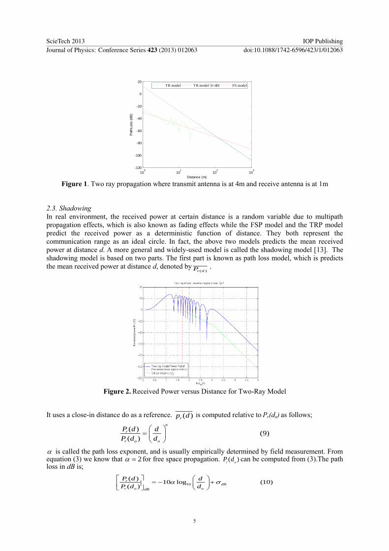