path integrals and symmetry breaking for optimal control
TRANSCRIPT

arX
iv:p
hysi
cs/0
5050
66 v
4 7
Oct
200
5
Path integrals and symmetry breaking for optimal control theory
H.J. Kappen
Radboud University,
Nijmegen, the Netherlands
December 30, 2005
Abstract
This paper considers linear-quadratic control of a non-linear dynamical system subject to arbitrarycost. I show that for this class of stochastic control problems the non-linear Hamilton-Jacobi-Bellmanequation can be transformed into a linear equation. The transformation is similar to the transforma-tion used to relate the classical Hamilton-Jacobi equation to the Schrodinger equation. As a result ofthe linearity, the usual backward computation can be replaced by a forward diffusion process, that canbe computed by stochastic integration or by the evaluation of a path integral. It is shown, how in thedeterministic limit the PMP formalism is recovered. The significance of the path integral approachis that it forms the basis for a number of efficient computational methods, such as MC sampling, theLaplace approximation and the variational approximation. We show the effectiveness of the first twomethods in number of examples. Examples are given that show the qualitative difference betweenstochastic and deterministic control and the occurrence of symmetry breaking as a function of thenoise.
1 Introduction
The problem of optimal control of non-linear systems in the presence of noise occurs in many areasof science and engineering. Examples are the control of movement in biological systems, robotics, andfinancial investment policies.
In the absence of noise, the optimal control problem can be solved in two ways: using the Pontrya-gin Minimum Principle (PMP) [1] which is a pair of ordinary differential equations that are similar tothe Hamilton equations of motion or the Hamilton-Jacobi-Bellman (HJB) equation which is a partialdifferential equation [2].
In the presence of Wiener noise, the PMP formalism can be generalized and yields a set of coupledstochastic differential equations, but they become difficult to solve due to the boundary conditions atinitial and final time (see however [3]). In contrast, the inclusion of noise in the HJB framework ismathematically quite straight-forward. However, the numerical solution of either the deterministic orstochastic HJB equation is in general difficult due to the curse of dimensionality. Therefore, one isinterested in efficient methods for solving the HJB equation. The class of problems considered belowallows for such efficient methods.
In section 3.1, we consider the control of an arbitrary non-linear dynamical system with arbitrarycost, but with the restriction, that the control acts linearly on the dynamics and the cost of the control
1

Figure 1: The drunken spider. In the absence of noise (alcohol in this case), the optimal trajectory forthe spider is to walk over the bridge. When noise is present, there is a significant probability to fall offthe bridge, incurring a large cost. Thus, the optimal noisy control is to walk around the lake.
is quadratic. For this class of problems, the non-linear Hamilton-Jacobi-Bellman equation can be trans-formed into a linear equation by a log transformation of the cost-to-go. The transformation stems backto the early days of quantum mechanics and was first used by Schrodinger to relate the Hamilton-Jacobiformalism to the Schrodinger equation. See section 7 for a further discussion on this point. The logtransform was first used in the context of control theory by [4] (see also [5]).
Due to the linear description, the usual backward integration in time of the HJB equation can bereplaced by computing expectation values under a forward diffusion process. This is treated in section 3.2.The computation of the expectation value requires a stochastic integration over trajectories that can bedescribed by a path integral (section 3.3). This is an integral over all trajectories starting at x, t, weightedby exp(−S/ν), where S is the cost of the path (also know as the Action) and ν is the size of the noise.It has the characteristic form of a partition sum and one should therefore expect that for different valuesof the noise ν the control is qualitatively different, and that symmetry breaking occurs below a criticalvalue of ν.
In general, control problems may have several solutions, corresponding to the different local minimaof S. The case is illustrated in fig. 1. A spider wants to go home, by either crossing a bridge or by goingaround the lake. In the absence of noise, the route over the bridge is optimal since it is shorter. However,the spider just came out of the local bar, where it had been drinking heavily with its friends. He is notquite sure about the outcome of its actions: any of its movements may be accompanied by a randomsway to the left or right. Since the bridge is rather narrow, and spiders don’t like swimming, the optimaltrajectory is now to walk around the lake. Thus, we see that the optimal control in the presence of noisecan be quantitatively different from the deterministic control.
2

In addition to which path to chose, the spider also has the problem when to make that decision. Faraway from the lake, he is in no position to chose for the bridge or the detour, as he is still uncertain ofwhere his random swaying may bring him. In other words, why would he spend control effort now tomove left or right when there is a 50 % change that he may wander there by chance? He decides to delayhis choice until he is closer to the lake. The question is, when should he make his decision to move leftor right?
It is in these multi-modal examples, that the difference between deterministic and stochastic controlbecomes most apparent. They are not only of concern to spiders, but occur quite general in obstacleavoidance for autonomous systems, differential games, and predator-prey scenarios. Current efficientapproaches to control are essentially restricted to unimodal situations and therefore cannot address theseissues. The aim of the present paper is to introduce a class of multimodal control problems that can beefficiently solved using path integral methods.
The path integral formulation is well-known in statistical physics and quantum mechanics, and severalmethods exist to compute them approximately. The Laplace approximation approximates the integral bythe path of minimal S and is treated in section 4. This approximation is exact in the limit of ν → 0, andthe deterministic control law is recovered. The formalism is illustrated for the linear quadratic case insection 4.2. Further refinements to the Laplace approximation can be made by considering the quadraticfluctuations around the deterministic solution (also know as the semi-classical approximation), but Ibelieve that this correction has a small effect on the control (it does strongly affect the value of J butnot its gradient). The semi-classical approximation is not treated in this paper.
As is shown in section 4.3, in the Laplace approximation the optimal stochastic control becomes amixture of deterministic control strategies, weighted by exp(−S/ν) and can be computed efficiently, Thepath integral displays a symmetry breaking at a critical value of ν: For large ν, the optimal control isthe average of the deterministic controls. For small ν, one of the deterministic controls is chosen. Insection 6.1.2 we give the example of the delayed choice problem that displays such symmetry breakingas a function of the time to reach the target.
In general, the Laplace approximation may not be sufficiently accurate. Possibly the simplest alterna-tive is Monte Carlo (MC) sampling. The naive sampling procedure proposed by the theory is presented insection 5.1, but is shown to be rather inefficient in the double slit example in section 6.1. It is not difficultto devise more efficient samplers. In section 5.2, we propose an importance sampling scheme, where thesampling distribution is a (mixture of) diffusion processes with drift given by the Laplace deterministictrajectories. The importance sampling method is compared with the exact results for the double slitproblem in section 6.1.1. In section 6.2, we compute the optimal control for the drunken spider for lownoise using the Laplace approximation and for high noise using MC importance sampling.
We begin our story with a brief derivation of the HJB equation for stochastic optimal control, whichis treated in depth in many good textbooks (see for instance [6, 5, 3]).
2 Stochastic optimal control
Consider the stochastic differential equation
dx = b(x(t), u(t), t)dt + dξ. (1)
x, b, dξ and dx are n-dimensional vectors and u is an m-dimensional vector of controls. dξ is a Wienerprocesses with 〈dξkdξl〉 = νkl(x, u, t)dt. The initial state of x is fixed: x(ti) = xi and the state at final
3

time tf is free. The problem is to find a control trajectory u(t), ti < t < tf , such that
C(xi, ti, u(·)) =
⟨
φ(x(tf )) +
∫ tf
ti
dtf0(x(t), u(t), t)
⟩
xi
(2)
is minimal. The subscript xi on the expectation value is to remind us that the expectation is over allstochastic trajectories that start in xi.
The standard construction of the solution for this problem is to set up a partial differential equationthat is to be solved for all times in the interval ti to tf and for all x. For this purpose, we define theoptimal cost-to-go function from any intermediate time t and state x:
J(x, t) = minu(t→tf )
C(x, t, u(t → tf )) (3)
where u(t → tf ) denotes the sequence of controls u(·) on the time interval [t, tf ]. For any intermediatetime t′, t < t′ < tf we can write a recursive formula for J in the following way:
J(x, t) = minu(t→tf )
⟨
φ(x(tf )) +
∫ t′
t
dtf0(x(t), u(t), t) +
∫ tf
t′dtf0(x(t), u(t), t)
⟩
x
= minu(t→t′)
⟨
∫ t′
t
dtf0(x(t), u(t), t) + minu(t′→tf )
⟨
φ(x(tf )) +
∫ tf
t′dtf0(x(t), u(t), t)
⟩
x(t′)
⟩
x
= minu(t→t′)
⟨
∫ t′
t
dtf0(x(t), u(t), t) + J(x(t′), t′)
⟩
x
(4)
The first line is just the definition of J . In the second line, we split the minimization over two intervals.These are not independent, because the second minimization is conditioned on the starting value x(t′),which depends on the outcome of the first minimization. The last line uses again the definition of J .
Setting t′ = t+ dt we can Taylor expand J(x(t′), t′) around t. This expansion takes place within theexpectation value and need to be performed to first order in dt and second order in dx, since
⟨
dx2⟩
=O(dt). This is the standard Ito calculus argument. Thus,
〈J(x(t+ dt), t+ dt)〉x =
⟨
J(x, t) + ∂tJ(x, t)dt + (∂xJ(x, t))T dx+1
2Tr(
∂2xJ(x, t)dx2
)
⟩
= J(x, t) + ∂tJ(x, t)dt+ (∂xJ(x, t))T b(x, u, t)dt+1
2Tr(
∂2xJ(x, t)ν(x, u, t)
)
dt
In this expression, ∂t and ∂x denotes partial differentiation with respect to t and x, respectively. Similarly,
∂2xJ is the matrix of second derivatives of J and Tr(ν∂2
xJ) =∑
ij νij∂2J
∂xi∂xj. Substituting this into Eq. 4,
dividing both sides by dt and taking the limit of dt → 0 yields
− ∂tJ(x, t) = minu
(
f0(x, u, t) + b(x, u, t)T∂xJ(x, t) +1
2Tr(
ν(x, u, t)∂2xJ(x, t)
)
)
, ∀t, x (5)
which is the Stochastic Hamilton-Jacobi-Bellman Equation with boundary condition J(x, tf ) = φ(x).
4
Eq. 5 reduces to the deterministic HJB equation in the limit ν → 0. In that case, an alternativeapproach to solving the control problem is the Pontryagin Maximum principle (PMP), which requiresthe solution of 2n ordinary differential equations. These equations need to be solved with multi-pointboundary conditions at both ti and tf . Solving 2n ordinary differential equations may be more efficientthan solving the n-dimensional partial differential equation, using shooting methods (see for instance [7]),but may be unstable in some cases.
In the stochastic case, there does not exist a generic alternative to solving the pde (see however [3]for stochastic versions of the PMP approach). Thus, for stochastic control one needs to solve the HJBequation, which suffers from the curse of dimensionality.
A notable exception is when b is linear in x and u and f0 is quadratic in x and u. This is calledthe linear-quadratic (LQ) control problem. In that case, it can be shown that the solution for J(x, t)is quadratic in x with time-varying coefficients. These coefficients satisfy coupled ordinary differential(Ricatti) equations that can be solved efficiently [6].
3 A path integral formulation for control
3.1 A linear HJB equation
Consider the special case of Eqs. 1 and 2 where the dynamic is linear in u and the cost is quadratic in u:
dx = (b(x, t) +Bu)dt+ dξ (6)
C(xi, ti, u(·)) =
⟨
φ(x(tf )) +
∫ tf
ti
dt
(
1
2u(t)TRu(t) + V (x(t), t)
)⟩
xi
(7)
with B an n × m matrix and R an m × m matrix. B, R and ν are independent of x, u, t. b and Vare arbitrary functions of x and t and φ is an arbitrary function of x. In other words, the system tobe controlled can be arbitrary complex and subject to arbitrary complex costs. The control instead, isrestricted to the simple LQ form.
The stochastic HJB equation 5 becomes
−∂tJ = minu
(
1
2uTRu+ V + (b+Bu)T∂xJ +
1
2Tr(
ν∂2xJ)
)
Minimization with respect to u yields:
u = −R−1BT ∂xJ(x, t) (8)
which defines the optimal control u for each x, t. The HJB equation becomes
−∂tJ = −1
2(∂xJ)TBR−1BT∂xJ + V + bT∂xJ +
1
2Tr(
ν∂2xJ)
This partial differential equation must be solved with boundary condition J(x, tf ) = φ(x). Note, thatafter performing the minimization with respect to to u, the HJB equation has become non-linear in J .
We can remove the non-linearity and this will turn out to greatly help us to solve the HJB equation.Define ψ(x, t) through J(x, t) = −λ logψ(x, t), with λ a constant to be defined. Then
−1
2(∂xJ)TBR−1BT∂xJ +
1
2Tr(
ν∂2xJ)
5

= − λ2
2ψ2
∑
ij
(∂xψ)i(BR−1BT )ij(∂xψ)j +
λ
2ψ2
∑
ij
νij(∂xψ)i(∂xψ)j −λ
2ψ
∑
ij
νij∂2ψ
∂xi∂xj
The terms quadratic in ψ vanish if and only if there exists a scalar λ such that
ν = λBR−1BT (9)
In other words, the matrices ν and BR−1BT must be proportional to each other with proportionalityconstant λ. In the one dimensional case, such a λ always exists, and Eq. 9 is not a restriction. In thehigher dimensional case, Eq. 9 restricts the possible choices for the matrices R and ν. To get an intuitionfor this restriction, consider the case that u and x have the same dimension, B is the identity matrix andboth R and ν are diagonal matrices. Then Eq. 9 states R ∝ ν−1. In a direction with low noise, controlis expensive (Rii large) and only small control steps are permitted. In the limiting case of no noise, wededuce that u should be set to zero: no control is allowed in noiseless directions. In noisy directions thereverse is true: control is cheap and large control values are permitted. Loosely speaking, Eq. 9 statesthat noise and control should operate in the same dimensions. 1
When Eq. 9 holds, the quadratic terms in the HJB equation cancel and the HJB becomes
∂tψ =
(
V
λ− bT∂x − 1
2Tr(ν∂2
x)
)
ψ
= −Hψ (10)
with H a linear operator acting on the function ψ. Eq. 10 must be solved backwards in time withψ(x, tf ) = exp(−φ(x)/λ). However, the linearity allows us to reverse the direction of computation,replacing it by a diffusion process, as we will explain in the next section.
To simplify the exposure in the subsequent sections, we assume the control dimension m = n and Bthe unit matrix.
3.2 Forward diffusion
For real functions ρ and ψ, define the inner product 〈ρ|ψ〉 =∫
dxρ(x, t)ψ(x, t). Then we can define H†,the Hermitian conjugate of the operator H , with respect to this inner product as follows.
⟨
H†ρ|ψ⟩
= 〈ρ|Hψ〉 =
∫
dxρ(x, t)
−V (x, t)
λ+ b(x, t)∂x +
1
2
∑
ij
νij∂2
∂xi∂xj
ψ(x, t)
1As a natural example, consider a one-dimensional second order system subject to additive control θ = f(θ, t) + u. Thefirst order formulation is obtained by setting x1 = θ and x2 = θ. Then
dxi = (bi(x, t) + Biu)dt, i = 1, 2
with b1(x, t) = x2, b2(x, t) = f(x1, t) and B = (0, 1)T . Since u is one-dimensional, R is a scalar and
BR−1BT =1
R
(
0 00 1
)
Condition Eq. 9 states that the stochastic dynamics must have the noise restricted to the second component only:
dxi = (bi(x, t) + Biu)dt + dξδi,2, i = 1, 2
with⟨
dξ2⟩
= νdt and λ = νR.
6

=
∫
dx
−V (x, t)
λρ(x, t) − ∂x(b(x, t)ρ(x, t)) +
1
2
∑
ij
νij∂2
∂xi∂xjρ(x, t)
ψ(x, t)
where we have performed integration by parts and assume that ρ vanishes at |x| → ∞. Thus,
H†ρ = −V (x, t)
λρ(x, t) − ∂x(b(x, t)ρ(x, t)) +
1
2
∑
ij
νij∂2
∂xi∂xjρ(x, t).
Let ρ(y, τ |x, t) be a probability density, initialized at t, x, that evolves forward in time according to thediffusion process
∂tρ = H†ρ (11)
with drift b(x, t)dt and diffusion dξ, and with an extra term due to the potential V . Whereas the other twoterms conserve probability density, the potential term takes out probability density at a rate V (x, t)dt/λ.Therefore, the stochastic simulation of Eq. 11 is a diffusion that runs in parallel with the annihilationprocess:
dx = b(x, t)dt+ dξ
x = x+ dx, with probability 1 − V (x, t)dt/λ
xi = †, with probability V (x, t)dt/λ (12)
where † denotes that the particle is taken out of the simulation. Note that when V = 0 this diffusionprocess is identical to the original control dynamics Eq. 6 in the absence of control (u = 0).
Since ψ evolves backwards in time according to H and ρ evolves forwards in time according to H† theinner product
∫
dyρ(y, τ |x, t)ψ(y, τ) is time invariant (independent of τ). Since ρ(y, t|x, t) = δ(y − x), itimmediately follows that
ψ(x, t) =
∫
dyρ(y, tf |x, t)ψ(y, tf ) (13)
We arrive at the important conclusion that ψ(x, t) can be computed either by backward integration usingEq. 10 or by forward integration of a diffusion process given by Eq. 11. The optimal cost-to-go is finallygiven by
J(x, t) = −λ log
∫
dyρ(y, tf |x, t) exp(−φ(y)/λ) (14)
with ρ(y, tf |x, t) given by the stochastic process Eq. 12. The optimal control is given by Eq. 8. Seesection 4.2 for a simple Gaussian example that illustrate these ideas.
3.3 The path integral formulation
In this section, we will write the diffusion kernel ρ(y, tf |x, t) in Eq. 14 as a path integral. For aninfinitesimal time step ǫ, we can write the probability to go from x to y as an integral over all noiserealizations. The probability of the Wiener is Gaussian with mean zero and variance νǫ. The particleannihilation destroys probability with rate V (x, t)ǫ/λ. Combining annihilation with diffusion, we obtain
ρ(y, t+ ǫ|x, t) ∝ exp
(
− ǫ
λ
[
1
2
(
y − x
ǫ− b(x, t)
)T
R
(
y − x
ǫ− b(x, t)
)
+ V (x, t)
])
7

where we have used ν−1 = R/λ.We can write the transition probability as a product of n infinitesimal transition probabilities:
ρ(y, tf |x, t) ∝∫
dx1 . . . dxn−1
exp
(
− ǫ
λ
n−1∑
i=0
[
1
2
(
xi+1 − xi
ǫ− b(xi, ti)
)T
R
(
xi+1 − xi
ǫ− b(xi, ti)
)
+ V (xi, ti)
])
In the limit of ǫ → 0, the sum in the exponent becomes an integral: ǫ∑n−1
i=0 →∫ tf
tdτ and thus we can
formally write
ρ(y, tf |x, t) =
∫
[dx]yx exp
(
− 1
λSpath(x(t → tf ))
)
(15)
Spath(x(t → tf )) =
∫ tf
t
dτ
(
1
2
(
dx(τ)
dτ− b(x(τ), τ)
)T
R
(
dx(τ)
dτ− b(x(τ), τ)
)
+ V (x(τ), τ)
)
(16)
with x(t → tf ) a path with x(τ = t) = x, x(τ = tf ) = y,∫
[dx]yx an integral over paths that start at xand end at y. 2
Substituting Eq. 15 in Eq. 14 we can absorb the integration over y in the path integral and find
J(x, t) = −λ log
∫
[dx]x exp
(
− 1
λS(x(t → tf ))
)
(17)
where the path integral∫
[dx]x is over all trajectories starting at x and
S(x(t → tf )) = φ(x(tf )) + Spath(x(t → tf )) (18)
is the Action associated with a path.The path integral Eq. 17 is a log partition sum and therefore can be interpreted as a free energy.
The partition sum is not over configurations, but over trajectories. S(x(t → tf )) plays the role of theenergy of a trajectory and λ is the temperature. This link between stochastic optimal control and a freeenergy has two immediate consequences. 1) Phenomena that allow for a free energy description, typicallydisplay phase transitions and spontaneous symmetry breaking. What is the meaning of these phenomenafor optimal control? 2) Since the path integral appears in other branches of physics, such as statisticalmechanics and quantum mechanics, we can borrow approximation methods from those fields to computethe optimal control approximately. First we discuss the small noise limit, where we can use the Laplaceapproximation to recover the PMP formalism for deterministic control. Also, the path integral showsus how we can obtain a number of approximate methods: 1) one can combine multiple deterministictrajectories to compute the optimal stochastic control 2) one can use a variational method, replacing theintractable sum by a tractable sum over a variational distribution and 3) one can design improvementsto the naive MC sampling.
2The paths are continuous but non-differential and there are different forward are backward derivatives [8, 9]. Therefore,the continuous time description of the path integral and in particular x are best viewed as a shorthand for its finite n
description.
8

4 The Laplace approximation
4.1 The Laplace approximation
When λ is small (i.e. ν is small), we can expand an arbitrary path x(τ) around the classical path:
x(τ) = x(τ) + δ(τ), t < τ < tf
where x(τ) is the classical path that we need to determine, and δ(τ) is an independent fluctuation of thepath at time τ . Fluctuations are also allowed at τ = t and τ = tf . The Action Eq. 18 can be expandedto first order in δ(τ) as
S(x(t→ tf )) = S(x(t → tf )) + δi(tf )∂iφ(x(tf ))
+
∫ tf
t
dτ
(
(x(τ) − b(x, τ))iRij
(
d
dτδj(τ) − δk(τ)∂kbj(x, τ)
)
+ δi(τ)∂iV (x(τ), τ)
)
= S(x(t → tf )) + δi(tf ) (∂iφ(x(tf )) + pj(tf )) − pj(t)δj(t)
−∫ tf
t
dτδk(τ)
(
d
dτpk(τ) + pj(τ)∂kbj(x, τ) − ∂kV (x(τ), τ)
)
(19)
where ∂k means partial differentiation with respect to xk, repeated indices are summed over and p isdefined as
pk(t) = (x(t) − b(x, t))jRjk (20)
The term proportional to δk(τ) under the integral must be zero and defines an ODE for the classicaltrajectory:
d
dtpk(t) +
∂
∂xk(pj(t)bj(x, t) − V (x, t)) = 0 (21)
Eq. 20 can be seen as a definition of p, but also as a dynamical equation for x that must be solvedtogether with the dynamical equation for p, Eq. 21. These equations must be solved with boundaryconditions. The boundary condition for x is given at initial time and the term proportional to δi(tf )defines the boundary condition for p(t) at t = tf :
xi(t) = x, pj(tf ) = −∂φ(x(tf ))
∂xj(22)
Define the Hamiltonian,
H(x, p, t) =1
2pTR−1p+ pT b(x, t) − V (x, t) (23)
Then, Eqs. 20 and 21 can be written as
dx
dt=∂H(x, p, t)
∂p,
dp
dt= −∂H(x, p, t)
∂x(24)
The Hamiltonian system Eqs. 24 with the mixed boundary conditions Eqs. 22 are the well-known ordinarydifferential equations of the Pontryagin Maximum Principle.
9

In the Laplace approximation, the path integral Eq. 17 is replaced by the classical trajectory only.Thus,
J(t, x) ≈ S(x(t → tf ))
since fluctuations at initial time are zero: δi(t) = 0. The optimal control is given by
u = −R−1∂xJ ≈ −R−1 δS(x(t → tf ))
δx(t)= R−1p(t) = x(t) − b(x(t), t) (25)
where we have usedδS(x(t→tf ))
δx(t) = −p(t) from Eq. 19. The intuition of the Laplace approximation is that
one needs to solve the deterministic equations for the whole interval [t, tf ], starting at the current placex. In particular, the end boundary condition (the location of the target) will affect the location of theoptimal path for all [t→ tf ]. The control is then given by the value of the pseudo-gradient x(t)−b(x(t), t)on this trajectory.
Note the minus sign in front of V in Eq. 23, which has the opposite sign from a normal classicalmechanical system. The term 1
2pTR−1p can be interpreted as the kinetic energy of the system. Thus,
the ’energy’ H is not the sum, but the difference of kinetic and potential energy. When H does notexplicitly depend on time (b(x, t) = b(x) and V (x, t) = V (x)), H is conserved under the deterministiccontrol dynamics:
dH
dt=∂H
∂x
dx
dt+∂H
∂p
dp
dt= 0
because of Eqs. 24. To understand this behavior, consider b = 0. Then along the trajectory:
1
2uTRu = V (x) +H
with H independent of time. This relation states that the optimal trajectory is such that much controlis spent in areas of large cost and little control is spent in areas of low cost.
Note, that the optimal control is independent of the noise ν as we expect from the Laplace approx-imation. Numerically, we can compute the classical trajectory by discretizing xcl(τ) = x1, . . . , xn andminimizing S(xcl) = S(x1, . . . , xn) using a standard minimization method.
4.2 The linear quadratic case
To build a bit of intuition for the diffusion process, the path integral and Laplace approximation, weconsider in this section some simple one-dimensional linear quadratic examples.
First consider the simplest case of free diffusion:
V (x, t) = 0, b(x, t) = 0, φ(x) =1
2αx2
In this case, the forward diffusion described by Eq. 11 and 12 can be solved in closed form and is givenby a Gaussian with variance σ2 = ν(tf − t):
ρ(y, tf |x, t) =1√2πσ
exp
(
− (y − x)2
2σ2
)
(26)
10

Since the end cost is quadratic, the optimal cost-to-go Eq. 14 can be computed exactly as well. Theresult is
J(x, t) = νR log
(
σ
σ1
)
+1
2
σ21
σ2αx2 (27)
with 1/σ21 = 1/σ2 + α/νR. The optimal control is computed from Eq. 8:
u = −R−1∂xJ = −R−1σ21
σ2αx = − αx
R+ α(tf − t)
We see that the control attracts x to the origin with a force that increases with t getting closer to tf .Note, that the optimal control is independent of the noise ν. This is a general property of LQ control.
As an extension, we now add a quadratic potential to the above problem: V (x) = 12µx
2. We nowcompute the optimal control in the Laplace approximation. The Hamiltonian is given by Eq. 23
H(x, p) =1
2R−1p2 − 1
2µx2
and the equations of motion and boundary conditions are given by Eqs. 24 and 22:
x = p/R p = µx
x(t) = x p(tf ) = −αx(tf )
We can write this as the second order system in terms of x only:
x = µx/R, x(t) = x x(tf ) = −αx(tf )/R
The solution for t < τ < tf is
x(τ) = Ae√
µ/R(τ−t) +Be−√
µ/R(τ−t)
The boundary conditions become A + B = x and Aγ(√
µ/R + α/R) = B/γ(√
µ/R − α/R), γ =
e√
µ/R(tf−t) from which we can solve A and B. The classical Action Eq. 18 is computed by substi-tuting the solution for x :
S(x(t → tf )) =1
2αx(tf )2 +
1
2
∫ tf
t
dτ(Rx2(τ) + µx2(τ)) =1
2
√
µRx2γ2 −
√µR−α√µR+α
γ2 +
√µR−α√µR+α
which is equal to the cost-to-go in the Laplace approximation. The optimal control is minus the gradientof the cost-to-go. Note, that the classical trajectory as well as the minimal action only depends on theinitial condition x and the time-to-go tf − t. For pure diffusion (µ→ 0) the classical Action reduces to
S(x(t→ tf )) =1
2
αRx2
R+ α(tf − t)
which is identical to the exact expression Eq. 27 except for the volume factor (which does not affect thecontrol, since it does not depend on x).
11

4.3 The multi-modal Laplace approximation
The Action S in Eq. 17 may have more than one local minimum. This is typical for control problems,where ”many roads lead to Rome”. Let xα(t → tf ), α = 1, . . . denote the different optimal deterministictrajectories that we compute by minimizing the Action:
xα(t→ tf ) = argminx(t→tf )S(x(t→ tf )), α = 1, . . .
These trajectories all start at the same value x. In our drunken spider example, there are two trajectories:one is over the bridge and the other is around the lake. Then, in the Laplace approximation the pathintegral Eq. 17 is approximated by these local minima contributions only:
J(x, t) ≈ −λ log∑
α
exp(−S(xα(t→ tf )/λ) (28)
The Laplace approximation ignores all fluctuations around the mode. Although these fluctuations can bequite big, their x dependence is typically quite weak and must come from beyond Gaussian corrections.This can be seen from the pure LQ case when the Gaussian fluctuation term in Eq. 27 is independent of x.In the LQ case, the Laplace approximation for the control (not for the cost-to-go) coincides with the exactsolution. Therefore, for unimodal problems (S has only one minimum) one can often safely ignore thecontribution of fluctuations to the control. However, for multi-modal problems these fluctuation termsmay have a strong α dependence (they have in the spider problem) and therefore play an important rolewhen weighting the different contributions in Eq. 28.
The optimal control becomes a soft-max of deterministic strategies
u(x, t) = −R−1∑
α
wα∂xS(xα(t→ tf )
wα =e−S(xα(t→tf )/λ
∑
β e−S(xβ(t→tf )/λ
where ν plays the role of the temperature.
5 MC sampling
A natural method for computing the optimal control is by stochastic sampling. However, as is often thecase with MC sampling, a naive sampler such as the one based directly on Eqs. 12 may be very inefficient.In this section, we show how this naive sampler works and how it can be improved using importancesampling.
5.1 Naive MC sampling
The stochastic evaluation of Eq. 13 consists of running N times the diffusion process Eq. 12 from t to tfinitialized each time at x(t) = x. Denote these N trajectories by xi(t → tf ), i = 1, . . . , N . Then, ψ(x, t)is estimated by
ψ(x, t) =∑
i∈alive
wi, wi =1
Nexp(−φ(xi(tf ))/λ) (29)
12

where ’alive’ denotes the subset of trajectories that do not get killed along the way by the † operation.Note that, although the sum is typically over less than N trajectories, the normalization 1/N includesall trajectories in order to take the annihilation process properly into account.
The computation of u requires the gradient of ψ(x, t) instead of ψ itself. First note, that when wevary the initial point of a path x(t → tf ) from Eq. 19 and 20 we obtain
δS(x(t → tf ))
δx(t)= (x(t) − b(x, t))R
Thus combining Eq. 8 and Eq. 17, we obtain
u =1
ψ(x, t)
∫
[dx]x(x(t) − b(x, t)) exp(−S/λ)
Note, that we can sample u by the same batch of (naive) trajectories. For each trajectory, the quantityx(t)− b(x, t) is proportional to the realisation of the noise in the initial time t: x(t)− b(x, t) = dξi(t)/dt.Therefore,
udt =1
ψ(x, t)
N∑
i∈alive
widξi(t) (30)
with wi given by Eq. 29. This expression has a particular intuitive form. The optimal control at time tis obtained by averaging the initial noise directions of the trajectories dξi(t), weighted by their successwi at the final time tf .
5.2 Importance sampling
The sampling procedure as described by Eqs. 12 and 29 gives an unbiased estimate of ψ(x, t) but canbe quite inefficient. The problem is is well known, and one of the simplest procedures for improving thesampling is by importance sampling. For path integrals this works as follows. We replace the diffusionprocess that yields ρ(y, tf |x, t) with Action Spath (Eqs. 15 and 16) by another diffusion process, that willyield ρ′(y, tf |x, t) with corresponding Action S′
path . Then,
ψ(x, t) =
∫
[dx]x exp (−Spath/λ) exp (−φ/λ)
=
∫
[dx]x exp(
−S′path/λ
)
exp(
−(φ+ Spath − S′path)/λ
)
The idea is to chose the diffusion process ρ′ such as to make the sampling of the path integral as efficientas possible.
A suggestion that comes to mind immediately is to use the Laplace approximation to compute adeterministic control trajectory x∗(t → tf ). From this, compute its derivative x∗(t → tf ) and define astochastic process to sample ρ′ according to
dx = x∗(t)dt+ dξ
x = x+ dx, with probability 1 − V (x, t)dt/λ
xi = †, with probability V (x, t)dt/λ (31)
13

The Action S′path for the Laplace-guided diffusion is given by Eq. 16 with b(x(τ), τ) = x∗(τ), t < τ < tf .
The estimators for ψ and u are given again by Eqs. 29 and 30, with the difference that
wi =1
Nexp
(
−(
φ(xi(tf )) + Spath(xi(t → tf )) − S′path(xi(t→ tf ))
)
/λ)
(32)
and xi(t → tf ) is a trajectory from the sampling process Eq. 31 instead of Eq. 12. We will illustrate theeffectiveness of this approach in section 6.1.
6 Numerical examples
In this section, we introduce some simple one-dimensional examples to illustrate the methods introducedin this paper. The first example is a double slit, and is sufficiently simple that we can compute theoptimal control by forward diffusion in closed form. We use this example to compare the Monte Carloand Laplace approximations to the exact result. Using the double slit example, we show how the optimalcost-to-go undergoes symmetry breaking as a function of the noise and/or some other characteristics ofthe problem (in this case the time-to-go). When the targets are still far in the future, the optimal controlis to ’steer for the middle’ and delay the choice to a later time.
The second example is similar to the first, except that the slit is now of finite thickness, allowing theparticle to get lost in one of the holes. When one hole is narrow and the other wide, this illustrates thedrunken spider problem. We use both the Laplace approximation and the the Monte Carlo importancesampling to compute the optimal control strategy, for different noise levels.
6.1 The double slit
Consider a stochastic particle that moves with constant velocity from t to tf in the horizontal directionand where there is deflecting noise in the x direction:
dx = udt+ dξ
The cost is given by Eq. 7 with φ(x) = 12x
2 and V (x, t1) implements a slit at an intermediate time t1,t < t1 < tf :
V (x, t1) = 0, a < x < b, c < x < d
= ∞, else
The problem is illustrated in Fig. 2a where the constant motion is in the t direction and the noise andcontrol is in the x direction perpendicular to it.
Eq. 9 becomes λ = νR and the linear HJB becomes:
∂tψ =
(
V
λ− ν
2∂2
x
)
ψ
which we must solve with end condition ψ(x, tf ) = e−φ(x)/λ.Solving this equation by means of the forward computation using Eq. 13 can be done in closed form.
First consider the easiest case for times t > t1 where we do not have to consider the slits. This is thecase we have considered before in section 4.2 and the solution is given by Eq. 27 with α = 1.
14

0 0.5 1 1.5 2
−6
−4
−2
0
2
4
6
8
t
x
(a) The double slit
−10 −5 0 5 100
1
2
3
4
5
x
J
t=0t=0.99t=1.01t=2
(b) Cost-to-go J(x, t)
Figure 2: (a) The particle moves horizontally with constant velocity from t = 0 to tf = 2 and is deflectedup or down by noise and control. The end cost φ(x) = x2/2. A double slit is placed at t1 = 1 with openingsat −6 < x < −4 and 6 < x < 8. Also shown are two example trajectories under optimal control. (b)J(x, t) as a function of x for t = 0, 0.99, 1.01, 2 as computed from Eq. 27 and 33. R = 0.1, ν = 1, dt = 0.02.
Secondly, consider t < t1. ρ(y, tf |x, t) can be written as a diffusion from t to t1, times a diffusion fromt1 to tf integrating over all x in the slits. Substitution in Eq. 13 we obtain
ψ(x, t) =
∫
dy
(
∫ b
a
+
∫ d
c
)
dx1 exp(−y2/2λ)ρ(y, tf |x1, t1)ρ(x1, t1|x, t)
ρ(y, tf |x1, t1) is Gaussian and given by Eq. 26. Therefore, we can perform the integration over y in closedform. We are left with an integral over x1 that can be expressed in terms of Error functions. The resultis
J(x, t) = νR log
(
σ
σ1
)
+1
2
σ21
σ2x2 − νR log
1
2(F (b, x) − F (a, x) + F (d, x) − F (c, x)) (33)
with F (x0, x) = Erf(√
A2ν (x0 − B(x)
A ))
, A = 1t1−t + 1
R+tf−t1and B(x) = x
t1−t . Eqs. 27 and 33 together
provide the solution for the control problem in terms of J and we can compute the optimal control fromEq. 8.
A numerical example for the solution for J(x, t) is shown in fig. 2b. The two parts of the solution(compare t = 0.99 and t = 1.01) are smooth at t = t1 for x in the slits, but discontinuous at t = t1 outsidethe slits. For t = 0, the cost-to-go J is higher around the right slit than around the left slit, because theright slit is further removed from the optimal target x = 0 and thus requires more control u and/or itsexpected target cost φ is higher.
15

0 0.5 1 1.5 2−10
−5
0
5
10
(a) Sample trajectories
−10 −5 0 5 100
2
4
6
8
10
x
J
MCExact
(b) MC sampling estimate of J(x, 0)
Figure 3: Monte Carlo sampling of J(x, t = 0) with ψ from Eq. 12 for the double slit problem. Theparameters are as in fig. 2. (a) Sample of trajectories that start at x to estimate J(x, t). Only trajectoriesthat pass through a slit contribute to the estimate. (b) MC estimate of J(x, t) = 0 with N = 100000trajectories for each x.
6.1.1 MC sampling
We assess the quality of the naive MC sampling scheme, as given by Eqs. 12 and 29 in fig. 3, where wecompare J(x, 0) as given by Eq. 33 with the MC estimate Eq. 29. The left figure shows the trajectories ofthe sampling procedure for one particular value of x. Note, the inefficiency of the sampler because mostof the trajectories are killed at the infinite potential at t = t1. The right figure shows the accuracy of theestimate of J(x, 0) for all x between −10 and 10 using N = 100000 trajectories. Note, that the numberof trajectories that are required to obtain accurate results, strongly depends on the value of x and λ dueto the factor exp(−φ(x)/λ) in Eq. 12. For high λ or low 〈φ〉, few samples are required (see the estimatesaround x = −4). For small noise or high 〈φ〉 the estimate is strongly determined by the trajectory withminimal φ(x(tf )) and many samples may be required to reach this x. In other words, sampling becomesmore accurate for high noise, which is a well-known general feature of sampling. Also, low values of thecost-to-go are more easy to sample accurately than high values. This is in a sense fortunate, since theobjective of the control is to move the particle to lower values of J so that subsequent estimates becomeeasier.
The sampling is of course particularly difficult in this example because of the infinite potential thatannihilates most of the trajectories. However, similar effects should be observed in general due to themulti-modality of the Action.
We can improve the sampling procedure using the importance sampling procedure outlined in sec-tion 5.2, using the Laplace approximation. The Laplace approximation to J requires the computationof the optimal deterministic trajectories. In general, one must use some numerical method to computethe Laplace approximation, for instance minimizing the Action Eq. 18 using a time-discretized versionof the path. In this particular example, however, we can just write down the classical trajectories ’byhand’. For each x, there are two trajectories, each being piecewise linear. The Action for each trajectory
16

−10 −5 0 5 100.5
1
1.5
2
2.5
3
x
J
Figure 4: Comparison of Laplace approximation (dotted line) and Monte Carlo importance sampling(solid jagged line) of J(x, t = 0) with exact result Eq. 33 (solid smooth line) for the double slit problem.The importance sampler used N = 100 trajectories for each x. The parameters are as in fig. 2.
is simply
Si(x) =1
2R
∫ 2
0
dtxi(t)2 =
R
2(ai − x)2 +
R
2a2
i , i = 1, 2
since φ(x(tf )) = V (x(t1), t1) = 0 by construction. ai = 6 and −4 for the two trajectories, respectively.The cost-to-go in the Laplace approximation is given by Eq. 28:
JLaplace(x, 0) = −νR log
(
exp
(
−S1(x)
λ
)
+ exp
(
−S2(x)
λ
))
For each x, we randomly choose one of the two Laplace approximations with equal probability. We thensample according to Eq. 31 with x∗ the selected Laplace approximation and estimate ψ using Eq. 29 andweights Eq. 32. The Laplace approximation and the results of the importance sampler are given in fig. 4.We see that the Laplace approximation is quite good for this example, in particular when one takes intoaccount that a constant shift in J does not affect the optimal control. The MC importance samplerdramatically improves over the naive MC results in fig. 3, in particular since 1000 times less samples areused and is also significantly better than the Laplace approximation.
6.1.2 The delayed choice
Finally, we show an example how optimal stochastic control exhibits spontaneous symmetry breaking.To simplify the mathematics, consider the double slit problem, when the size of the slits becomes in-finitesimally small. Eq. 33, with a = 1, b = 1 + ǫ, c = −1 − ǫ, d = −1 becomes to lowest order inǫ:
J(x, t) =R
T
(
1
2x2 − νT log 2 cosh
x
νT
)
+ const.
where the constant diverges as O(log ǫ) independent of x and T = t1 − t the time to reach the slits. Theexpression between brackets is a typical free energy with inverse temperature β = 1/νT . It displays a
17

−2 −1 0 1 20.4
0.6
0.8
1
1.2
1.4
1.6
1.8
x
J(x,
t)
T=2
T=1
T=0.5
(a) Optimal cost-to-go at different T .
0 0.5 1 1.5 2−2
−1
0
1
2stochastic
0 0.5 1 1.5 2−2
−1
0
1
2
0 0.5 1 1.5 2−2
−1
0
1
2deterministic
0 0.5 1 1.5 2−2
−1
0
1
2
(b) Sample paths
Figure 5: (a) Symmetry breaking in J as a function of T implies a ’delayed choice’ mechanism for optimalstochastic control. When the target is far in the future, the optimal policy is to steer between the targets.Only when T < 1/ν should one aim for one of the targets. ν = R = 1. (b) Sample trajectories (top row)and controls (bottom row) under stochastic control Eq. 34 (left column) and deterministic control Eq. 34with ν = 0 (right column), using identical initial conditions x(t = 0) = 0 and noise realization.
symmetry breaking at νT = 1 (fig. 5a). For T > 1/ν (far in the past) it is best to steer towards x = 0(between the targets) and delay the choice which slit to aim for until later. The reason why this is optimalis that from that position the expected diffusion alone of size νT is likely to reach any of the slits withoutcontrol (although it is not clear yet which slit). Only sufficiently late in time (T < 1/ν) should one makea choice. The optimal control is given by the gradient of J :
u =1
T
(
tanhx
νT− x)
(34)
Figure 5b depicts two trajectories and their controls under stochastic and deterministic optimal con-trol, using the same realization of the noise. Note, that at early times the deterministic control drives xaway from zero whereas in the stochastic control drives x towards zero and smaller in size. The stochasticcontrol maintains x around zero and delays the choice for which slit to aim until T ≈ 1.
The fact that symmetry breaking occurs in terms of the value of νT , is due to the fact that S ∝ 1/T ,which in turn is due to the fact that u ∝ 1/T . Clearly, this will not be true in general. For an arbitrarycontrol problem, S does not need to be monotonic in T , which means that in principle control can beshifting back and forth several times between the symmetric and the broken mode as T decreases to zero.
6.2 The drunken spider
In order to illustrate the drunken spider problem, we change the potential of the double slit problem sothat it has a finite thickness: V (x, t) = 0 for all t < t1 and t > t2 and for t1 < t < t2:
V (x, t) = 0, a < x < b, c < x < d
18

= ∞, else (35)
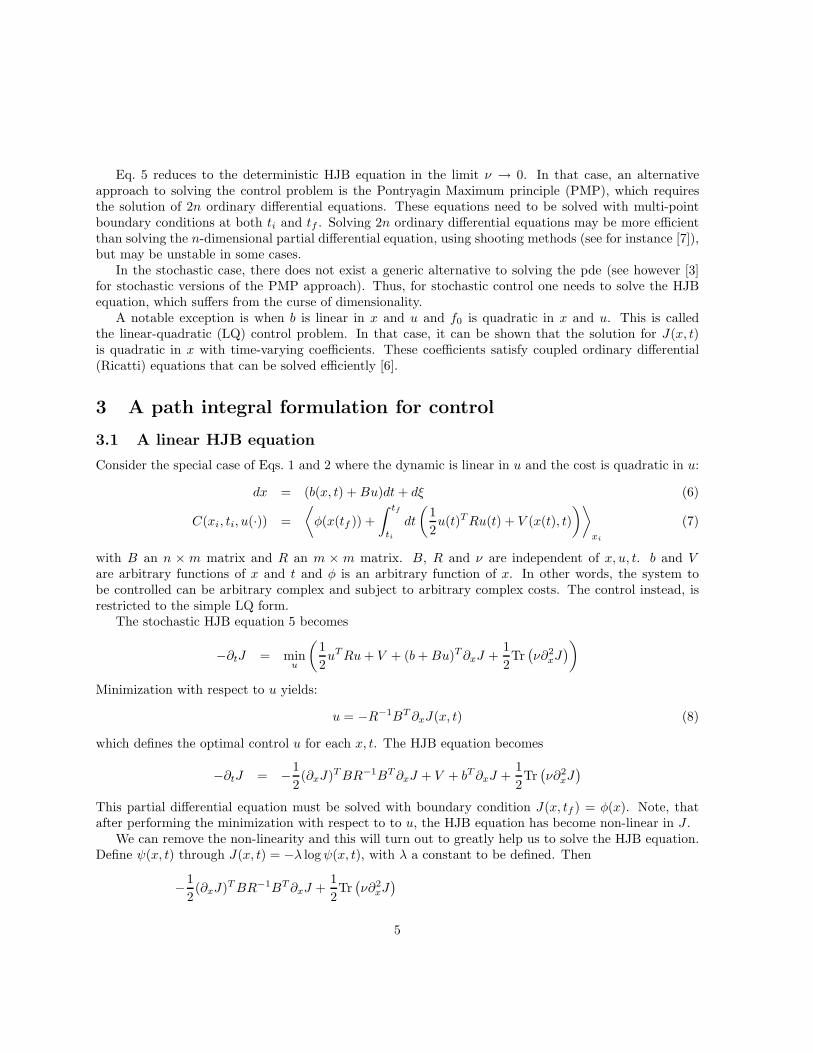
The problem is illustrated in Fig. 6 and the parameter values are given in the caption.The cost-to-go in the Laplace approximation is given by Eq. 28, with S(x(α(t → tf )), α = 1, 2 the
cost of getting home over the bridge or around the lake, respectively. It is plotted as a function of thecurrent position x as the solid line in fig. 6c, for both ν = 0.001 and ν = 0.1 (these two curves coincidefor these values of ν, since S/ν is so large that the softmax is basically a max).
In addition, we compute J using importance sampling as outlined in section 5.2. For each x, we runm = 1000 trajectories. For each trajectory, we select randomly one of the two Laplace trajectories withequal probability, which we denote by x∗(t→ tf ). The stochastic trajectory x(t→ tf ) is then computedfrom Eq. 31. It contributes to the partition sum Eq. 29 with a weight that is computed by Eq. 32, whereSpath(x(t → tf )) and S′
path(x(t → tf )) are given by Eq. 16 with b(x(τ), τ) = 0 and b(x(τ), τ) = x∗(τ),respectively.
The results of the MC importance sampling for various x for low noise (ν = 0.001) and high noise(ν = 0.1) are also shown in fig. 6c. The dots are the results of the MC importance sampling at low noiseand closely follow the Laplace results. Note the discontinuous change in slope at x = −6, which impliesa discontinuous change in the optimal control value u at that point: For x > −6 the spider steers forthe bridge, which requires a larger control value than for x < −6 when the optimal trajectory is aroundthe lake. Thus, the optimal path is simply given by the shortest path and noise is ignored in theseconsiderations.
The MC estimates for ν = 0.1 are indicated by the stars in fig. 6c. Since noise is large, the Laplaceapproximation is not valid, and indeed are very different from the MC estimate. The Laplace approxi-mation ignores the effect of deviations from the deterministic trajectory on the Actions . Thus, it doesnot take into account that the spider may wander off the bridge and drowns, which at this level of noisewill happen with almost probability one and makes Sbridge much larger than Slake. The MC importancesampling is guided by trajectories around the lake, that likely survive and by trajectories over the bridge,that will likely drown and thus will not contribute to Eq. 29. The estimate for J is thus dominatedby trajectories around the lake and the cost-to-go increases with increasing x. Also note, that the MCestimate puts the minimum of J not at x = −6 but safely away from the lake, so that spider is not likelyto fall in the lake on the low side either, and will have a safe journey home.
7 Discussion
In this paper, we have addressed the problem of computing stochastic optimal control. The direct solutionof the HJB equation requires a discretization of space and time. This computation naturally becomesintractable in both memory requirement and cpu time in high dimensions. We have shown, that for acertain class of problems the control can be computed by a path integral. The class of problems includesarbitrary dynamical systems, but with a limited control mechanism. It includes LQ control as a specialcase. The path integral approach has the advantage that the n-dimensional x-space integration of theHJB equation is replaced by an n-dimensional sampling problem. For high-dimensional problems, astochastic integration method is expected to be much more efficient than numerical integration of theHJB equation directly, which scales exponentially in n.
The obvious approximation methods to use are the Laplace approximation, the variational approxi-mation and MC sampling. The Laplace approximation is very efficient. The deterministic trajectories arefound by minimizing the action, which can be done by standard numerical methods. It typically requires
19
−1 0 1 2 3 4 5−10
−8
−6
−4
−2
0
2
t
x
(a) Sample paths for ν = 0.001
−1 0 1 2 3 4 5−10
−8
−6
−4
−2
0
2
t
x(b) Sample paths for ν = 0.1
−10 −5 0 50
10
20
30
40
50
x
J
(c) J(x, t = −1)
Figure 6: The drunken spider problem. A spider located at x and t = −1 wants to arrive home (x = 0)at time tf . The lake is indicated by the white square area, interrupted by a narrow bridge. Thelake is modelled by the infinite potential given by Eq. 35 with −a = b = 0.1, c = −∞ and d = −6.t1 = 0, t2 = 4, tf = 5 and R = 1. The cost-to-go is computed by forward importance sampling as outlinedin section 5.2. The guiding Laplace approximations are the deterministic trajectories over the bridge andaround the lake. Time discretization dt = 0.012. (a) Some stochastic trajectories used to compute J forν = 0.001. (b) Some stochastic trajectories used to compute J for ν = 0.1. (c) The optimal cost-to-goJ(x, t) in the Laplace approximation for ν = 0.001 and ν = 0.1 solid line (these two curves coincide).The MC importance sampling estimates are based on 1000 trajectories per x for ν = 0.001 (dots) andfor ν = 0.1 (stars).
20

O(n2k2) operations, where n is the dimension of the problem and k is the number of time discretizations.We have seen that the multi-modal Laplace approximation gives non-trivial solutions involving symmetrybreaking.
Computing the path integral by MC sampling is clearly a very generic approach, that for manypractical control applications may well be the best way to go. Naive sampling should be replaced bymore advanced sampling schemes. I have only considered one simple improvement using importancesampling. Other possible improvements could be a Gibbs sampler or a Metropolis-Hasting sampler.Clearly, more work in this direction must be done.
In this paper we have numerically computed the path integrals using the most simple discretizationstrategy: short time averaging [10]. The computation can be made much more efficient using Fourierdiscretization [11, 12] or other subspace approximations (compact splines or wavelets) [13]. In each ofthese methods the path integral is reduced to a high (but finite) dimensional Riemann integral, which isapproximated using a Monte Carlo method. These more advanced discretizations can be combined withany of the mentioned MC methods.
I have not discussed the variational approximation in this paper. This approach to approximating thepath integral is also known as variational perturbation theory and gives an expansion of the path integralin terms of the anharmonic interaction terms and a variational function that is to be optimized [14]. Thelowest term in the expansion is similar to what is known as the variational approximation in machinelearning using the Jensen’s bound [15], but one can also consider higher order terms. The expansion isaround a tractable dynamics, such as for instance the harmonic oscillator, whose variational parametersare optimized such as to best approximate the path integral. The application of this method to optimalcontrol would be the topic of another paper. A complication of such an analytic treatment is the presenceof topological constraints, such as walls and obstacles.
There exist other fields of research that use path integrals and where dedicated numerical methodshave been developed to solve them. For instance, in chemical physics path integrals are used to describeconformational changes in molecules over large time scales. The problem is similar to an optimal controlproblem such as navigating a maze: The begin and end positions are known, and one or more path ofminimal cost needs to be found. A prominent method in this field is transition path sampling [16], whichcan be viewed as a Metropolis-Hasting sampling scheme in path space, where a new path is sampledby changing part of the current path and accepting the new path with a probability. This approach isprobably also suitable for optimal control.
There is a superficial relation between the work presented in this paper and the body of work that seeksto find a particle interpretation of quantum mechanics. In fact, the log transformation was motivatedfrom that work. Madelung [17] observed that if Ψ =
√ρ exp(iJ/h) is the wave function that satisfies the
Schrodinger equation, ρ and J satisfy two coupled equations. One equation describes the dynamics of ρas a Fokker -Planck equation. The other equation is a Hamilton-Jacobi equation for J with an additionalterm, called the quantum-mechanical potential which involves ρ. Nelson showed that these equationsdescribe a stochastic dynamics in a force field given by the ∇J , where the noise is proportional to h[8, 18].
Comparing this to the relation Ψ = exp(−J/λ) used in this paper, we see that λ plays the role of h asin the QM case. However, the big difference is that there is only one real valued equation, and not twoas in the quantum mechanical case. In the control case, ρ is computed as an alternative to computingthe HJB equation. In the QM case, the dynamics of ρ and J are computed together. The QM densityevolution is non-linear in ρ because the drift force that enters the Fokker-Planck equation depends on ρthrough J as computed from the HJ equation.
21

Acknowledgement
I would like to thank Hans Maassen for useful discussions. I would like to thank Michael Jordan, PeterBartlett and Stuart Russell to host my sabbatical at UC Berkeley, which gave me the time to writethis paper. This work is sponsored in part by the Miller Institute for Basic Research in Science of theUniversity of California at Berkeley and the ICIS project, grant number BSIK03024.
References
[1] L.S. Pontryagin, V.G. Boltyanskii, R.V. Gamkrelidze, and E.F. Mishchenko. The mathematical theory of
optimal processes. Interscience, 1962.
[2] R. Bellman and R. Kalaba. Selected papers on mathematical trends in control theory. Dover, 1964.
[3] J Yong and X.Y. Zhou. Stochastic controls. Hamiltonian Systems and HJB Equations. Springer, 1999.
[4] W.H. Fleming. Exit probabilties and optimal stochastic control. Applied Math. Optim., 4:329–346, 1978.
[5] W.H. Fleming and H.M. Soner. Controlled Markove Processes and Viscosity solutions. Springer Verlag, 1992.
[6] R. Stengel. Optimal control and estimation. Dover publications, New York, 1993.
[7] L.F. Shampine, I. Gladwell, and S. Thompson. Solving ODEs with MATLAB. Cambridge University Press,2003.
[8] E. Nelson. Dynamical Theories of Brownian Motion. Princeton University Press, Princeton, 1967.
[9] F. Guerra. Introduction to nelson stochastic mechanics as a model for quantum mechanics. In The Foundation
of Quantum Mechanics, Amsterdam, 1995. Kluwer.
[10] K.S. Schweizer, R.M. Stratt, D. Chandler, and P.G. Wolynes. Convenient and accurate discretized pathintegral methods for equilibrium quantum mechanical calculations. J.Chem. Phys., 75:1347–1364, 1981.
[11] W.H. Miller. Path integral representation of the reaction rate constant in quantum mechanical transitionstate theory. J.Chem. Phys., 63:1166–1172, 1975.
[12] D.L. Freeman and J.D. Doll. A monte carlo method for quantum boltzmann statistical mechanics usingfourier representations of path integrals. J.Chem. Phys., 80:5709–5718, 1984.
[13] S.D. Bond, B.B. Laird, and B.J. Leimkuhler. On the approximation of feynman-kac path integrals. Journal
of Computational Physics, 185:472–483, 2003.
[14] H. Kleinert. Path integrals in quantum mechanics, statistics,polymer physics and financial markets. MITPress, 2004. Third edition.
[15] R.P. Feynman and H. Kleinert. Effective classical partition functions. Physical Review A, 34:5080–5084,1986.
[16] P.G. Bolhuis, D. Chandler, Ch. Dellago, and P.L. Geissler. Transition path sampling: Throwing ropes overrough mountain passes, in the dark. Annu. Rev. Phys. Chem., 53:291–318, 2002.
[17] E. Madelung. Z. Physik, 40:322, 1926.
[18] F. Guerra. Structural aspects of stochastic mechanics and stochastic field theory. Physics Reports, 77:263–312, 1981.
22