Path Following with an Optimal Forward Velocity

for a Mobile Robot

Kiattisin Kanjanawanishkul, Marius Hofmeister, and Andreas Zell

Department of Computer Architecture, University of Tubingen, Sand 1, 72076Tubingen, Germany

(e-mail: {kiattisin.kanjanawanishkul, marius.hofmeister,andreas.zell}@uni-tuebingen.de)

Abstract: In this paper, we present a novel solution for a path following problem in partially-knownstatic environments. Given linearized error dynamic equations, model predictive control (MPC) isemployed to produce a sequence of angular velocities. Since the forward velocity of the robot has to beadapted to environmental constraints and robot dynamics while the robot is following a path, we proposean optimal solution to generate the velocity profile. Furthermore, we integrate an obstacle-avoidancebehavior using local sensor information with a path-following behavior based on global knowledge. Toachieve this, we introduce new waypoints in order to move the robot away from obstacles while the robotstill keeps following the desired path. Extensive simulations and experiments with a physical unicyclemobile robot have been conducted to illustrate the effectiveness of our path following control framework.

Keywords: Robot control, autonomous mobile robots, obstacle avoidance, path following, modelpredictive control.

1. INTRODUCTION

Fundamental problems of motion control of autonomous mo-bile robots can be roughly classified into three groups (Morinand Samson, 2008), namely point stabilization, trajectory track-ing, and path following. In this paper, we focus on the pathfollowing problem. Pioneering work in this area can be foundin (Micaelli and Samson, 1993). The underlying assumptionof this problem is that the robot’s forward velocity tracks adesired velocity profile, while the controller determines therobot’s moving direction to drive it to the path without any con-sideration in temporal specifications. Typically this controllereliminates the aggressiveness of the tracking controller by forc-ing convergence to the path in a smooth way (Al-Hiddabi andMcClamroch, 2002).

The path following problem has been well studied and manysolutions have been proposed and applied in a wide range ofapplications. Samson (Samson, 1995) described a path follow-ing problem for a car pulling several trailers. Altafini (Altafini,2002) addressed a path following controller for an n trailervehicle. Path following controllers for aircraft and marine ve-hicles were reported in (Al-Hiddabi and McClamroch, 2002)and (Encarnacao and Pascoal, 2000), respectively.

In this work, we wish to achieve three objectives: static obstacleavoidance, path following, and forward velocity selection. Anillustrative example for these objectives is car driving. A drivercontrols a car to follow a road using a steering maneuver.The driver may decelerate the car if he or she sees obstaclesblocking the road or is making a sharp turning, or is drivingon an icy road. Besides all these situations, safety concerns andhuman comfort also influence the desired forward velocity.

We separate our problem into three parts as shown in Fig. 1.The MPC block produces a sequence of angular velocities.

Its detail is given in Section 2. The velocity selection block,described in Section 3, adapts the forward velocity of the robotto environmental constraints and robot dynamics. The referencepath generator block, explained in detail in Section 4, providesthe desired reference for path following control and replansthe path if the robot moves close to obstacles. Simulationand experimental results are shown in Section 5. Finally, ourconclusions and future work are given in Section 6.

2. THE PATH FOLLOWING PROBLEM

In this section, the model predictive control (MPC) frameworkis used to generate a sequence of angular velocities. MPChas become an increasingly popular control technique used inindustry (Kwon and Han, 2005; Mayne et al., 2000). It is basedon a finite-horizon continuous time minimization of predictedtracking errors with constraints on the control inputs and thestate variables. At each sampling time, the model predictivecontroller generates an optimal control sequence by solvingan optimization problem. The first element of this sequence isapplied to the system. The problem is solved again at the nextsampling time using the updated process measurements and ashifted horizon.

Most model predictive controllers use a linear model of mobilerobot kinematics to predict future system outputs. In (Lages

and Alves, 2006; Klancar and Skrjanc, 2007), model-predictivecontrol based on a linear, time-varying description of the systemwas used for trajectory tracking control. Generalized predictivecontrol was used to solve path following control in (Ollero andAmidi, 1991). A nonlinear predictive controller for a trajectorytracking problem was proposed in (Gu and Hu, 2006). AnMPC-based approach for active steering control was imple-mented in (Falcone et al., 2007). The differences of this paperfrom other work are that (i) this paper deals with a linearizedmodel for path following control, (ii) we take into account

Fig. 1. The block diagram describes our solution for the path following control problem.

obstacle avoidance, and (iii) the forward velocity selection isintroduced.

In general, a linear MPC framework is computationally effec-tive and can be easily used in fast real time implementations.To apply this framework, we first formulate our problem. Thekinematics of a mobile robot, depicted in Fig. 2 together with aspatial path Γ to be followed, can be described by

xy

θ

=

[

v cos θv sin θω

]

(1)

where x(t) = [x, y, θ]T denotes the state vector in the worldframe. v and ω are the linear and angular velocities, respec-tively. We wish to find control law ω such that the robot con-verges to the path while v tracks velocity profiles. The patherror with respect to the path frame is given by

[

xe

yeθe

]

=

[

cos θd sin θd 0− sin θd cos θd 0

0 0 1

][

x− xd

y − ydθ − θd

]

(2)

where the state vector of the reference point, [xd, yd, θd]T , is

computed by using a numerical projection from the robot’scurrent state onto the path.

Then, the linearized version of the error dynamics xe =[ye, θe]

T (the lateral and angular deviations, respectively) re-sults in

ye = vdθe

θe = ω − ωd

(3)

where vd and ωd are the desired linear and angular velocities,respectively. We can transform the optimization problem ofMPC to a quadratic programming (QP) problem by using thislinearized model. Since it becomes a convex problem, solvingthe QP problem leads to global optimal solutions. Equation (3)can be given in the state-space form xe = Acxe + Bcue. Todesign the MPC controller for path following, the linearizedsystem (3) will be written in a discrete state space system as

xe(k + 1) = Axe(k) +Bue(k) (4)

where A ∈ Rn × R

n, n is the number of state variables andB ∈ R

n×Rm, m is the number of input variables. The discrete

matrices A and B can be obtained as follows:

A = I +AcTs

B = BcTs(5)

Fig. 2. A graphical representation of a mobile robot and a path.A small circle ◦ denotes a distance sensor.

where Ts is a sampling time.

Given a state space model (4) of a system, it is possible touse MPC to control it. To achieve this, we have to minimize aquadratic objective function by solving a quadratic program inorder to obtain control-variable values. The quadratic objectivefunction with a prediction horizon N is given by

J(k) =

N∑

j=1

{xTe (k + j|k)Qxe(k + j|k)

+ uTe (k + j − 1|k)Rue(k + j − 1|k)}

(6)

where Q ∈ Rn × R

n and R ∈ Rm × R

m are the weightingmatrices, with Q ≥ 0 and R ≥ 0. The double subscript notation(k+j|k) denotes the prediction made at time k of a value at timek+j. Furthermore, the matrix Q is adapted to lateral deviationsas follows

Q(1, 1) =c1

1 + c2|ye|(7)

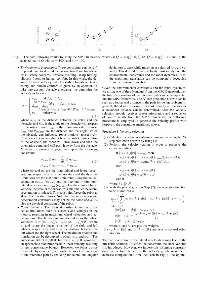
where c1 and c2 are positive. When the robot is far away fromthe path, the weighting gain for lateral deviations will becomesmaller, resulting in more importance in angular errors. Whenthe robot moves closer to the path, Q(1, 1) becomes larger,leading to more importance in lateral errors, as seen in Fig. 3.

After some algebraic manipulations, we can rewrite the objec-tive function (6) in a standard quadratic form:

J(k) =1

2UT (k)H(k)U(k) + fT (k)U(k) (8)

where U(k) = [uTe (k|k),uT

e (k+1|k), . . . ,uTe (k+N−1|k)]T .

The matrix H(k) ∈ Rm·N × R

m·N is a Hessian matrix and itis always positive definite. It describes the quadratic part of theobjective function and the vector f(k) ∈ R

m·N describes thelinear part. The unconstrained control law can be obtained byminimizing the objective function with respect to U as follows

∂J(k)

∂U(k)= H(k)U(k) + f(k) (9)

and the control vector becomes

U(k) = H−1(−f(k)) . (10)

This control vector contains a sequence of angular velocities.

3. FORWARD VELOCITY SELECTION

Besides steering the robot to the desired path, assigning a ve-locity profile to the robot can be an additional task, in whichthe forward velocity is used as an extra degree of freedom. Forexample, in (Bak et al., 2001), the forward velocity decreases asthe robot rotates around a sharp corner by scaling the forwardvelocity. In (Lapierre et al., 2007), the forward velocity is con-trolled when an obstacle is detected. In this paper, the velocityprofile is shaped to comply with environmental constraints androbot dynamics along some lookahead distance correspondingto the N -step prediction horizon of the MPC framework. Weconsider bounds on the forward velocity as follows:

−0.4 −0.2 0 0.2 0.4 0.6 0.8

0.1

0.2

0.3

0.4

0.5

0.6

0.7

0.8

(a)

0 0.2 0.4 0.6 0.8 1 1.20.4

0.5

0.6

0.7

0.8

0.9

1

1.1

1.2

(b)

0 0.2 0.4 0.6 0.8 1 1.2

0.4

0.5

0.6

0.7

0.8

0.9

1

1.1

1.2

(c)

Fig. 3. The path following results by using the MPC framework, where (a) Q = diag(100, 1), (b) Q = diag(10, 1), and (c) theadapted matrix Q with c1 = 1000 and c2 = 100.

• Environmental constraints: These constraints can be self-imposed due to desired behaviors based on high-leveltasks, safety concerns, obstacle avoiding, sharp turning,slippery floors, or human comfort. In this work, the de-sired forward velocity, which satisfies high-level tasks,safety, and human comfort, is given by an operator. Totake into account obstacle avoidance, we determine thevelocity as follows

v =

vmin if dobs < dminvd − vmin

dmax − dmin

(dobs − dmin) + vmin

if dmin ≤ dobs ≤ dmax and |θobs| < θobs,max

vd otherwise(11)

where dobs is the distance between the robot and theobstacle, and θobs is the angle of the obstacle with respectto the robot frame. dmin is the minimum safe distance.dmax and θobs,max are the distance and the angle, whichthe obstacle can influence robot motions, respectively.Equation (11) means that when the robot moves closeto the obstacle, the robot will slow down and then theorientation command will push it away from the obstacle.Moreover, to prevent slippage, we impose the followingconstraints

aT,min ≤ aT =dv

dt≤ aT,max

aL,min ≤ aL = κv2 ≤ aL,max

(12)

where aT and aL are the longitudinal and lateral accel-erations, respectively. κ is the curvature and the dynamiclimitations are the maximum (minimum) longitudinal ac-celeration aT,max (aT,min) and the maximum (minimum)lateral acceleration aL,max (aL,min). For the constant linearvelocity, the smaller the curvature is, the smaller the lateralacceleration is induced. This constraint forces the robot toslow down in sharp turns. Note that the acceleration anddeceleration constraints may not be the same and aT isalso the physical constraint of the robot.

• Robot dynamics: The physical constraints are due to theactual limitations such as currents and voltages in themotors, resulting in maximum wheel velocities and ac-celerations. The limitations are derived from the wheelvelocities: v = (vr + vl)/2, ω = (vr − vl)/(2b), wherevr and vl are the linear velocities of the right and leftwheels, respectively, and 2b is the distance between theleft wheel and the right wheel. The maximum rotation andtranslation can be decoupled to obtain vmax and ωmax. Theauthors in (Bak et al., 2001; Indiveri et al., 2007) proposedan approach to maximize feasible linear velocity, resultingin less conservative bounds. However, we focus on thedifferent objective, i.e., we wish the robot to convergeto the reference path by reducing the lateral and angular

deviations to zero while traveling at a desired forward ve-locity. This desired forward velocity must satisfy both theenvironmental constraints and the robot dynamics. Thus,the maximum translation can be completely decoupledfrom the maximum rotation.

Given the environmental constraints and the robot dynamics,we utilize one of the advantages from the MPC framework, i.e.,the future information of the reference path can be incorporatedinto the MPC framework. The N -step prediction horizon can beseen as a lookahead distance in the path following problem. Ingeneral, the slower a desired forward velocity is, the shortera lookahead distance can be determined. After the velocityselection module receives sensor information and a sequenceof control inputs from the MPC framework, the followingprocedure is employed to generate the velocity profile withrespect to the constraints mentioned above.

Procedure 1: Velocity selection

(1) Calculate the actual orientation commands ω along the N -step prediction horizon by using (3)

(2) Perform the velocity scaling in order to preserve thecurvature radius

if |ω(k + j|k)| > ωmax then

vp(k + j|k) = v(k + j|k)ωmax/|ω(k + j|k)|

ωp(k + j|k) = sign(ω(k + j|k))ωmax

else

vp(k + j|k) = v(k + j|k)

ωp(k + j|k) = ω(k + j|k)

end if

where j ∈ [0, N − 1](3) With the profile given in Step (2), the objective function

to be minimized is

mina,ε

( N∑

j=1

γ1‖vp(k + j|k)− vm(k + j|k)‖2 + γ2‖ε‖

)

s.t. 0 ≤ ε|κv2m(k + 1|k)| − aL,max ≤ ε

a(k + j|k) =vm(k + j + 1|k)− vm(k + j|k)

Ts|a(k + j|k)| ≤ aT,max

where γ1 and γ2 are positive weights(4) vp(k + 1|k) and ωp(k + 1|k) are sent to control robot

motions

The hard constraint of the lateral acceleration may lead to theinfeasible solution. To soften the constraint, the slack variableε is introduced. However, we impose this softening constraintonly on the first element of the velocity profile in order todecrease computational time. As seen in Fig. 4, the optimal

(a)

0 5 10 15−0.1

0

0.1

0.2

0.3

time (s)

m/s

0 5 10 15

−0.4

−0.2

0

0.2

0.4

0.6

time (s)

rad/s

(b) (c)

0 5 10 15−0.1

0

0.1

0.2

0.3

time (s)

m/s

0 5 10 15

−0.4

−0.2

0

0.2

0.4

0.6

time (s)

rad/s

(d)

Fig. 4. The path following results with aT,max = 0.2 m/s2, aL,max = 0.2 m/s2, ωmax = 0.5 rad/s, v0 = 0.2 m/s, and N = 50steps (the lookahead distance = 0.5 m and Ts = 0.05 s): (a) using the optimal velocity strategy, (b) the velocity profilescorresponding to (a), (c) using the constant forward velocity, and (d) the velocity profiles corresponding to (c).

velocity selection module can reduce the lateral deviations be-cause the robot moves at a lower velocity (see Fig. 4(b)) while itis making a sharp turning. Obviously, the lateral deviations in-crease, if the constant velocity is chosen, as shown in Fig. 4(c).

4. THE PATH REPLANNING STRATEGY

Typically, the desired reference is generated by a planning algo-rithm based on a map of the environment and this reference isassumed to be collision-free. During the movement in partiallystructured environments, an obstacle can suddenly appear onthe robot’s path, which had not been present in the planningphase. To avoid the obstacle, a sensory system should detect theobstacle, measure its distance and orientation for replanning therobot’s path. In (Lapierre et al., 2007), an obstacle avoidancealgorithm based on the use of a continuous Deformable VirtualZone (DVZ) is combined with a path following controller. In(Macek et al., 2009), global path planning, path following, anda collision avoidance scheme are integrated in a unified frame-work, namely the Traversability-anchored Dynamic Path Fol-lowing (TADPF). In this paper, we combine a path-followingbehavior using global knowledge with an obstacle-avoidancebehavior based on local sensor information. Furthermore, wekeep tracking the curvilinear abscissa s(t) ∈ R, which is usedto parameterize the reference path. This path’s parameter s canbe used to detect whether the robot is stuck in a loop and to leadthe robot back to the path when the obstacle-avoidance behaviorbecomes inactive.

The obstacle-avoidance behavior becomes active as the robotmoves closer to obstacles than dmax and one of these obstaclesblocks the robot. The path replanning module then locallygenerates new waypoints to deform the reference path in orderto bring the robot away from the obstacle. These new waypointsare tangential to the edges of the obstacle with an offset dr.Procedure 2 below describes our solution in detail.

Procedure 2: Path replanning strategy

(1) Receive sensor information, estimate the edges of all de-tected obstacles, and evaluate the number of the detectedobstacles. If the distance between two detected points islarger than the distance ds, a new obstacle is introduced.If it is smaller, it means the robot cannot get through.

(2) Create convex hulls around the obstacle edges with anoffset distance dr. If two polygons overlap, they are com-bined into one convex polygon (see Fig. 5(b) as an exam-ple).

(3) Evaluate the relevant obstacles, which influence robotmotions and then make a decision based on the generated

polygons around the detected obstacles and the referencepath to make a right turn or a left turn in order to avoid theobstacles.

(4) From Step (3), keep following on that side along the edgesof the convex polygon toward the first visible vertex (seeFig. 5(a) and Fig. 5(b) as examples) until that obstacle nolonger influences robot motions.

Note that the distances ds and dr are dependent on the robotsize and the sensor accuracy.

Fig. 6 illustrates the results from applying Procedure 2. “×”represents a detected point by a range sensor and dashed linesindicate the convex polygons around the detected points. How-ever, the robot may make a wrong decision in some situationsbecause of insufficient sensor information. For example, therobot may move far away from the reference path becauseit keeps following the boundary of the obstacle. In this case,global knowledge may be needed to solve this problem.

5. SIMULATION AND EXPERIMENTAL RESULTS

Our path following control framework has been evaluated inboth computer simulations written in MATLAB and a physicalunicycle mobile robot. To show the effectiveness of our ap-proach, the simulations were first conducted using an arbitrarilyconstructed environment including obstacles. We assume that

(a) (b)

Fig. 5. Two cases are shown as examples. A robot detectsan obstacle and convex hulls are then created aroundthe edges of the detected obstacle. The robot will followthe first visible vertex along the edges of the convexpolygon. (a) A convex polygon is constructed around anobstacle, and (b) a convex polygon covers two detectedobstacles because their convex polygons overlap. Dashedlines represent the replanned path and dotted lines are partof the convex polygons around the detected obstacles.

−5 −4 −3 −2 −1 0 1 2 3 4 5

−2

−1

0

1

2

3

t=0

x (m)

y (

m)

(a)

−2 −1.5 −1 −0.5 0 0.5 1 1.5 2

−1.5

−1

−0.5

0

0.5

1

1.5

t=0

x (m)

y (

m)

(b)

Fig. 7. The simulation results by using our path following control framework: (a) The robot starting at [4.5,−1.7, 2π/3]T isrequired to follow a reference path represented by thick lines, and (b) the robot starting at [0, 0.75,−π/4]T is required tofollow an eight-shaped curve. The polygons are obstacles while the small circles are snapshots of robot location every 2.5 s.The robot trajectories are shown as dashed curves.

prior knowledge of the workspace was available but the locationof all the static polygonal obstacles in the workspace were un-known to the robot. The robot was modeled as a small circle (12cm in diameter) and 12 virtual sensors mimic infra-red sensorsplaced in the form of a circle along the circumference of therobot. They were spaced by 30◦ and they had a distance rangeof 30 cm. In our implementation, we also applied hysteresis tothe state transition in order to avoid a chattering situation whenswitching between two behaviors occurs.

The user-defined parameters in the simulation were set asfollows

aT,max = 0.5 m/s2, aL,max = 0.5 m/s2, ωmax = 2 rad/s,v0 = 0.2 m/s, N = 50 steps, Ts = 0.05 s, dr = 0.2 m,dmax = 0.2 m, dmin = 0.1 m, θobs,max = 75◦, ds = 0.5 m,

Q(1, 1) =1000

1 + 100|ye|, Q(2, 2) = 1, R = 0.01.

3.2 3.4 3.6 3.8 4 4.2 4.4 4.6 4.8−2

−1.8

−1.6

−1.4

−1.2

−1

−0.8

−0.6

−0.4

−0.2

0

x (m)

y (

m)

(a)

3.4 3.6 3.8 4 4.2 4.4 4.6 4.8

−1.8

−1.6

−1.4

−1.2

−1

−0.8

−0.6

−0.4

−0.2

0

x (m)

y (

m)

(b)

Fig. 6. (a) The obstacle-avoidance behavior becomes activebecause sensor information indicates that there are threeobstacles detected and the one in front of the robot caninfluence the robot motion. Then, the path replanningmodule needs to decide that the robot should turn left orturn right. (b) The planner selects right turning. The robotkeeps following that obstacle on the right until no relevantobstacle is detected. When no obstacle is detected, thepath-following behavior becomes active; the robot keepsfollowing the reference path.

The simulation results obtained in complex scenarios withdifferent obstacle configurations are presented in Fig. 7. As seenin the results, it can be concluded that the robot successfullyfollows the reference path and avoids all obstacles. Noticethat in Fig. 7(a), the robot at coordinate (−4, 0) decided toturn left and then it was going to be caught in a trap. Thetrap was discovered by monitoring the path’s parameter. Ifthe path’s parameter before the obstacle-avoidance behaviorbecomes active is greater than the path’s parameter after theobstacle-avoidance behavior becomes inactive, this implies thatthe robot is very likely about to run in a closed loop. To avoidtrap-situations, the robot followed the obstacle at its right at thistime (see Fig. 7(a)).

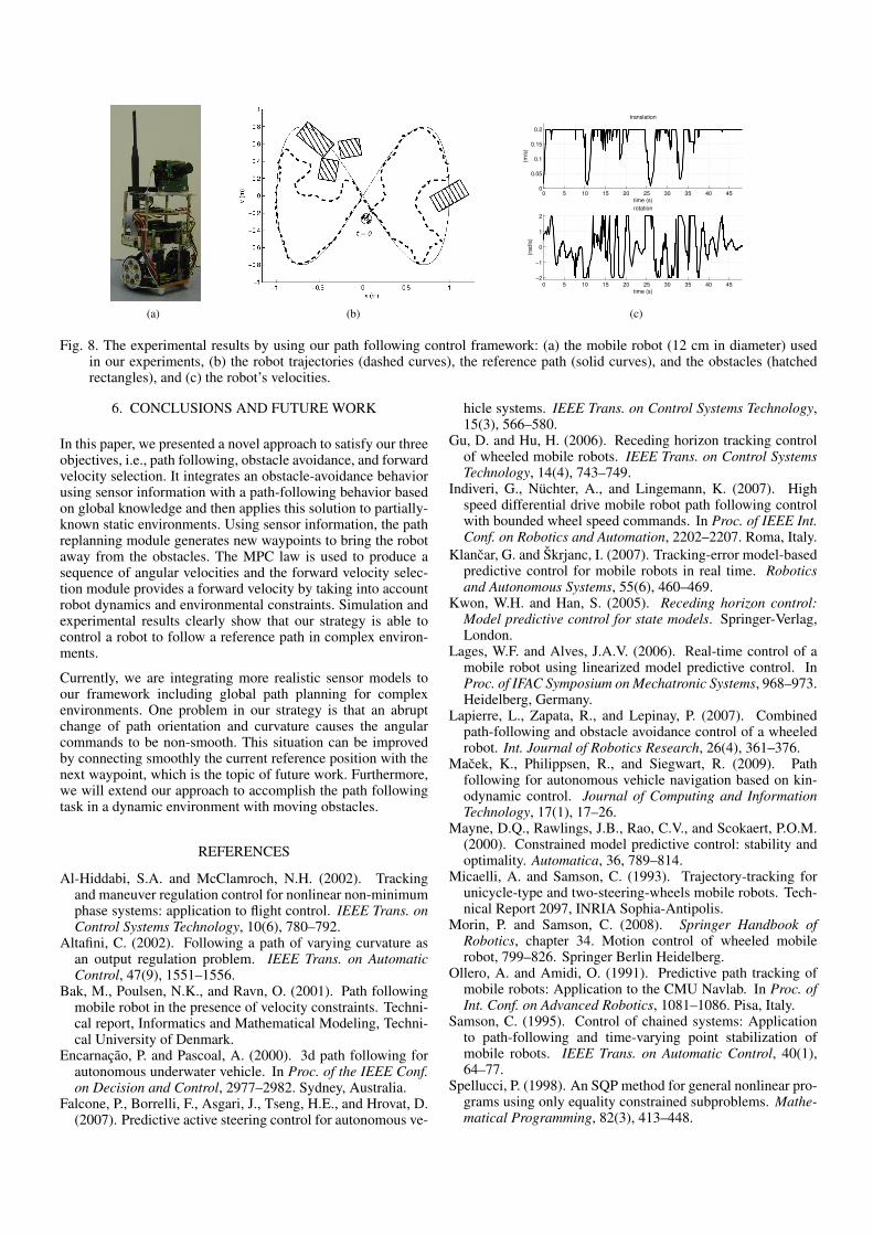
To show the usefulness of our approach, the unicycle-type mo-bile robot, shown in Fig. 8(a), was used in real-world experi-ments. The robot controller is an ATMEGA644 microprocessorwith 64 KB flash program memory, 16 MHz clock frequencyand 4 KB SRAM. The robot orientation was measured by aDevantech CMPS03 compass. The localization was given bya camera looking down upon the robot’s workplace and a PCwas used to compute control inputs and then sent these inputsto the robot via WLAN. An eight-shaped curve similar to thepath in the second simulation was employed in this experi-ment. Gaussian noise with a fixed variance was added to alldistance measurements, given by virtual distance sensors. Dueto high computational time in optimization solving, only 10steps were used for the prediction horizon and the cycle timewas set to 0.1 s. Our software was developed in C++ with theadditional use of some geometrical calculations from CGAL(Computational Geometry Algorithms Library - online avail-able: http://www.cgal.org). The free package DONLP2 (Spel-lucci, 1998) was used to solve the optimization problem.

The experimental results are plotted in Fig. 8(b). As depictedin Fig. 8(c), the robot was able to travel at the desired speedv0 = 0.2 m/s in case of no obstacle or no sharp turning curve.The velocity selection module optimized the forward and rota-tional velocities, if environmental and/or robot constraints wereviolated, while the path replanning module locally handled ob-stacle avoidance.

(a) (b)

0 5 10 15 20 25 30 35 40 450

0.05

0.1

0.15

0.2

translation

time (s)

(m/s

)

0 5 10 15 20 25 30 35 40 45−2

−1

0

1

2

rotation

time (s)

(ra

d/s

)

(c)

Fig. 8. The experimental results by using our path following control framework: (a) the mobile robot (12 cm in diameter) usedin our experiments, (b) the robot trajectories (dashed curves), the reference path (solid curves), and the obstacles (hatchedrectangles), and (c) the robot’s velocities.

6. CONCLUSIONS AND FUTURE WORK

In this paper, we presented a novel approach to satisfy our threeobjectives, i.e., path following, obstacle avoidance, and forwardvelocity selection. It integrates an obstacle-avoidance behaviorusing sensor information with a path-following behavior basedon global knowledge and then applies this solution to partially-known static environments. Using sensor information, the pathreplanning module generates new waypoints to bring the robotaway from the obstacles. The MPC law is used to produce asequence of angular velocities and the forward velocity selec-tion module provides a forward velocity by taking into accountrobot dynamics and environmental constraints. Simulation andexperimental results clearly show that our strategy is able tocontrol a robot to follow a reference path in complex environ-ments.

Currently, we are integrating more realistic sensor models toour framework including global path planning for complexenvironments. One problem in our strategy is that an abruptchange of path orientation and curvature causes the angularcommands to be non-smooth. This situation can be improvedby connecting smoothly the current reference position with thenext waypoint, which is the topic of future work. Furthermore,we will extend our approach to accomplish the path followingtask in a dynamic environment with moving obstacles.

REFERENCES

Al-Hiddabi, S.A. and McClamroch, N.H. (2002). Trackingand maneuver regulation control for nonlinear non-minimumphase systems: application to flight control. IEEE Trans. onControl Systems Technology, 10(6), 780–792.

Altafini, C. (2002). Following a path of varying curvature asan output regulation problem. IEEE Trans. on AutomaticControl, 47(9), 1551–1556.

Bak, M., Poulsen, N.K., and Ravn, O. (2001). Path followingmobile robot in the presence of velocity constraints. Techni-cal report, Informatics and Mathematical Modeling, Techni-cal University of Denmark.

Encarnacao, P. and Pascoal, A. (2000). 3d path following forautonomous underwater vehicle. In Proc. of the IEEE Conf.on Decision and Control, 2977–2982. Sydney, Australia.

Falcone, P., Borrelli, F., Asgari, J., Tseng, H.E., and Hrovat, D.(2007). Predictive active steering control for autonomous ve-

hicle systems. IEEE Trans. on Control Systems Technology,15(3), 566–580.

Gu, D. and Hu, H. (2006). Receding horizon tracking controlof wheeled mobile robots. IEEE Trans. on Control SystemsTechnology, 14(4), 743–749.

Indiveri, G., Nuchter, A., and Lingemann, K. (2007). Highspeed differential drive mobile robot path following controlwith bounded wheel speed commands. In Proc. of IEEE Int.Conf. on Robotics and Automation, 2202–2207. Roma, Italy.

Klancar, G. and Skrjanc, I. (2007). Tracking-error model-basedpredictive control for mobile robots in real time. Roboticsand Autonomous Systems, 55(6), 460–469.

Kwon, W.H. and Han, S. (2005). Receding horizon control:Model predictive control for state models. Springer-Verlag,London.

Lages, W.F. and Alves, J.A.V. (2006). Real-time control of amobile robot using linearized model predictive control. InProc. of IFAC Symposium on Mechatronic Systems, 968–973.Heidelberg, Germany.

Lapierre, L., Zapata, R., and Lepinay, P. (2007). Combinedpath-following and obstacle avoidance control of a wheeledrobot. Int. Journal of Robotics Research, 26(4), 361–376.

Macek, K., Philippsen, R., and Siegwart, R. (2009). Pathfollowing for autonomous vehicle navigation based on kin-odynamic control. Journal of Computing and InformationTechnology, 17(1), 17–26.

Mayne, D.Q., Rawlings, J.B., Rao, C.V., and Scokaert, P.O.M.(2000). Constrained model predictive control: stability andoptimality. Automatica, 36, 789–814.

Micaelli, A. and Samson, C. (1993). Trajectory-tracking forunicycle-type and two-steering-wheels mobile robots. Tech-nical Report 2097, INRIA Sophia-Antipolis.

Morin, P. and Samson, C. (2008). Springer Handbook ofRobotics, chapter 34. Motion control of wheeled mobilerobot, 799–826. Springer Berlin Heidelberg.

Ollero, A. and Amidi, O. (1991). Predictive path tracking ofmobile robots: Application to the CMU Navlab. In Proc. ofInt. Conf. on Advanced Robotics, 1081–1086. Pisa, Italy.

Samson, C. (1995). Control of chained systems: Applicationto path-following and time-varying point stabilization ofmobile robots. IEEE Trans. on Automatic Control, 40(1),64–77.

Spellucci, P. (1998). An SQP method for general nonlinear pro-grams using only equality constrained subproblems. Mathe-matical Programming, 82(3), 413–448.