1

Pass-through in dollarized countries: should Ecuador abandon

the U.S. Dollar?

María Lorena Marí del Cristo*a and Marta Gómez-Puig

b

March 2013

Abstract

In this article we examine the convenience of dollarization for Ecuador today. As

Ecuador is strongly integrated financially and commercially with the United States, the

exchange rate pass-through should be zero. However, we sustain that rising rates of

imports from trade partners other than the United States and subsequent real effective

exchange rate depreciations are causing the pass-through to move away from zero. Here,

in the framework of the Vector Error Correction Model, we analyse the impulse response

function and variance decomposition of the inflation variable. We show that the

developing economy of Ecuador is importing inflation from its main trading partners,

most of them emerging countries with appreciated currencies. We argue that if Ecuador

recovered both its monetary and exchange rate instruments it would be able to fight

against inflation. We believe such an analysis could be extended to other countries with

pegged exchange rate regimes.

JEL Classification: E31; F31; F41.

Keywords: Pass-through, shocks, dollarized countries, structural VECM.

The authors would like to express their gratitude to Andrea Cipollini, Barbara Pistoresi and Antonio Ribba for helpful

comments. a Department of Economics. University of Barcelona, Av.Diagonal 690. Barcelona 08034. Email:

lmari@ub.edu. b Department of Economics. University of Barcelona and RiskCenter-IREA, Av. Diagonal 690. Barcelona

08034. Email: marta.gomezpuig@ub.edu. This article is based upon work supported by the Government of Spain and

FEDER under grant number ECO2010-21787-C03-01. *Corresponding author: Lorena Marí. E-mail: lmari@ub.edu

2

I. Introduction

Selecting the optimal exchange rate regime for developing and emerging countries is the

subject of ongoing debate in international economic forums, especially in light of the

current global economic crisis that has called into question most exchange rate regimes1.

Given the variety of such regimes2, the exchange rate pass-through (ERPT) literature,

which examines the inflationary pressure attributable to the transmission mechanism of

the exchange rates, is presented as a useful framework for exploring the economic

implications of these regimes and identifying the most convenient exchange rate

mechanism for a given country. Here, we focus our study on the pegged exchange rate

regime adopted in Ecuador, a dollarized country which is currently undergoing major

political and economic changes that might result in changing its exchange rate regime in

the near future3.

In theory, dollarized countries should have a very low pass-through as their currencies are

anchored to that of their principal trade partner. In Ecuador, the appearance of

inflationary pressure due to pass-through might reflect the fact it has begun to substitute

its traditional trade partners. China, for example, was the leading merchandise exporter in

2010 ($1.58 trillion, or 10% of world exports) and accounted for 7.8% of Ecuador’s total

imports4. Fig. 1 in Appendix B shows the appreciation of the Chinese yuan (CNY)

against the US dollar (USD). When China reformed its fixed exchange rate regime to a

1Even the European Monetary Union, the benchmark for economies undertaking similar projects, has been questioned in

terms of a deficient political and fiscal union (Issing, 2011). 2Reinhart & Rogoff (2004) used market-determined exchange rates (from dual/parallel markets) and found fourteen

categories of exchange rate regimes, ranging from no separate legal tender or a strict peg to a dysfunctional “freely falling”

or “hyperfloat”. 3Ecuador is a member of major Latin American economic organizations including UNASUR

(www.uniondenacionessuramericanas.com), CAN (www.comunidadandina.org), ALBA (www.alianzabolivariana.org),

which in 2007 created the Bank of the South – a credit institution similar to the World Bank, and it is soon to join

MERCOSUR(MERCOSUR/CMC/DEC. Nº38/11). The aim of these organizations is to create a South American Free

Trade Area, using a new currency (the sucre), which was first used in 2010 as a virtual currency in at least two transactions

between Ecuador and Venezuela. Ecuador is also diversifying its trade partners, with Asian countries being its leading

exporters in 2010 (www.icex.es). 4Reported by the World Trade Organization in 2011 Press Releases (PRESS/628).

3

managed floating exchange rate system in July 20055, one USD was valued at 8.2700

CNY. In January 2012 one USD was worth 6.3548 CNY, an appreciation of 23.15%.

Likewise, the rates of appreciation experienced by two currencies belonging to two of

Ecuador’s main trade partners, Colombia and Japan, are shown in Fig. 2 (Appendix B).

In times of crisis, the ERPT plays a crucial role in achieving an internal and external

balance. When the ERPT is high, variations in the exchange rate result in changes in the

relative prices of tradable and non-tradable commodities generating a rapid adjustment in

the trade balance. At the same time, high ERPT also encourages domestic production to

substitute imported products.

In general, developing countries are heavily dependent on imports. These imported

products become more expensive following episodes of depreciation, thereby affecting

the economic growth of these countries in terms of levels of investment and consumption.

As developing countries are unlikely to renounce imported products, as the pass-through

rises, the rate of inflation with which they have to contend also grows. In a currency

crisis, therefore, developing countries find themselves most severely affected owing to

the deterioration in the balance sheet of financial institutions as they borrow in foreign

currencies from foreign institutions, but lend in the domestic currency to domestic firms.

If the national currency is depreciated these liabilities are magnified, and the banks are

unable to lend and investors send their profits abroad (capital flights), resulting in

contractionary effects in the economy6.

When a country is dollarized it can overcome a high ERPT coefficient and its balance-

sheet problems as long as the United States continues to be its principal lender and

commercial partner. Yet, what happens if this situation should change? Fig. 3 in

5This new system replaced the USD, which had served as the sole anchor currency for approximately ten years, with a

basket of currencies that was weighted to account for bilateral trade volume and bilateral investment. 6 Frankel (2005) in his article “Contractionary currency crashes in developing countries” describes how depreciations of the

national currency cause contractionary effects rather than an expansion in economies highly indebted in dollars.

4

Appendix B shows the evolution in Ecuador’s main suppliers over the period 1998 to

2010. Although United States remains the main trading country, Latin America is the

leader among the regions, comprising the Latin American Integration Association

(Argentina, Brazil, Chile, and Mexico) and the Andean Community (Bolivia, Colombia,

Peru and Venezuela). The figure also highlights the growth recorded by Asia (comprising

Japan, Taiwan, China and South Korea), which since 2004 has replaced Europe as the

third largest source of imports. Thus, as the trade relations between the two “monetary

linked” countries weaken, the benefits to the dollarized country of operating a pegged

exchange rate regime are reduced. Bastourre et al. (2003) found that if the financial

channel (FC) becomes a more important transmission mechanism than the trade channel

(TC), the FC will increase the gross domestic product (GDP) volatility of the dollarized

country7.

In conducting our research here, we selected a Latin American country, namely Ecuador,

which was dollarized in 2000 principally to avoid escalating inflationary pressures. The

study, undertaken in the framework of a Vector Error Correction Model (VECM),

examines a period that extends from January 2000 to July 2011 (i.e., covering ten years of

dollarization and part of the current global economic crisis).

The article is organized as follows. In the section that follows we provide a brief

economic history of Ecuador. In section three, we present an overview of the pass-

through literature, emphasizing the paucity of studies conducted for developing countries.

In sections four and five, we describe the theoretical framework and the data and

methodology adopted, respectively. Our empirical results are reported in section six and

we draw our conclusions in section seven

7 With business cycles negatively correlated, the FC increases real volatility and the TC reduces it. If the anchor country is

hit by a positive shock, two simultaneous processes will take place: a) the anchor country will increase imports from the

pegged country, positively affecting the GDP of this country through the TC, but b) since the anchor country could issue a

restrictive monetary policy in order to avoid over-heating, the increase in the interest rate will negatively affect the pegged

country through the FC.

5

II. Ecuador – a history of dollarization

The relative advantages and drawbacks of official dollarization to a country are well

documented8. Thus, this exchange rate regime facilitates the control of inflation and

interest rates, aids the stabilization of the exchange rate and ensures lower transaction

costs; however, the process also entails high transition costs, while a country loses control

over its monetary policy, its central bank no longer serves as a lender of last resort and,

ultimately, a national symbol is lost.

There are three different degrees of dollarization: unofficial and semi-official – both of

which are referred to as partial dollarization – and official or full dollarization. In Latin

America and the Caribbean region alone all three regimes can be found9. This study is

concerned with full dollarization in which the national currency is substituted by the US

dollar as legal tender. Below, we briefly outline the monetary history of Ecuador, the

country under analysis here.

Ecuador’s national currency, the sucre, first launched in 1884 by the government of Jose

Maria Placido Caamaño, was replaced as legal tender by the US dollar in 2000, at a rate

of 25 000 sucres per dollar. In the early 1990s, Ecuador introduced various structural

reforms that provided a certain degree of macroeconomic stability at least until the middle

of that decade. However, a number of endogenous shocks – including, an inefficient

fiscal policy and increasing financial dollarization – and exogenous shocks – including

the impact of the climate oscillation, el Niño, and international oil prices – immersed the

country in a period of economic stagnation that saw macroeconomic imbalances increase

(Jacome, 2004).

8 See Alesina and Barro (2001), De Nicoló, Honohan and Ize, (2005), and Berg and Borensztein, E. (2000). 9 Peru, Uruguay and Bolivia operate a high degree of financial dollarization (a variety of partial dollarization) in which

foreign assets exceed domestic assets but where each country maintains its own currency. Haiti operates a system of semi-

official dollarization in which the foreign currency is legal tender, but where it plays a secondary role to the domestic

currency for paying taxes and wages. Finally, only three countries are fully dollarized, namely, Ecuador, El Salvador and

Panama.

6

At the end of the twentieth century, Ecuador experienced one of the most serious crises in

the history of the Republic with inflation rates being recorded at 30 percent per month.

The government intervened in the banks and many public deposits were frozen.

Internationally, Ecuador’s standing was not good; it was in arrears with its private

creditors and bondholders, while the International Monetary Fund, the World Bank and

the Inter-American Development Bank withheld important loans that might have

supported the Ecuadorian balance of payments.

The country was in urgent need of radical measures that would stabilize expectations,

avoid acute currency depreciation and hyperinflation, and restore economic and financial

activity. At the same time, the government was in urgent need of radical measures that

would allow it to escape being overthrown. At its head, President Mahuad faced the

challenges of severe social and economic crisis - real GDP fell 7.3 percent,

unemployment rose from 11 to 15 percent and an active indigenous movement called for

political and economic reform. In an attempt to switch the focus from political issues to

economic matters, he concluded that the radical solution was dollarization.

Following dollarization, GDP rose by 2.3 percent in 2000, and climbed 5.4 percentage

points in 2001. Inflation had been stabilized, but at the same time international oil prices

recovered so the immediate effects of dollarization on Ecuador’s economy were

somewhat ambiguous. Today, Ecuador is a member of the Andean Community of

Nations (CAN), a free trade area, and most of the members have a floating exchange rate

regime. As such, Ecuador is at risk of experiencing what Argentina underwent when

Brazil devalued the real in 1999. Argentina, operating a currency board system, was

unable to adjust its exchange rate parity in order to recover competitiveness (Beckerman

and Solimano, 2002).

7

III. A brief overview of the pass-through literature

The study of exchange rate pass-through began with the “law of one price” and the

Purchasing Power Parity (PPP) literature. Dornbusch (1985), drawing on evidence

prepared for the New Palgrave dictionary of economics, presents an excellent definition

and review of this literature. Today, pass-through – the degree to which exchange rate

changes are passed through to price levels – has been identified as the main mechanism

providing theoretical support for deviations from PPP. Since the 1980s, various empirical

studies have examined ERPT to domestic prices (including import, producer and

consumer prices), yet most of the literature has focused its attention on industrialized

countries.

At the micro level, Dornbusch (1987) applied industrial organization models to explain

the relationship between exchange rate fluctuations and domestic price changes, in terms

of market structure – import share and concentration – and the substitutability of imports

for domestic products. The lower the level of product substitutability in an industry, and

the greater the share of foreign exporters relative to domestic producers, the greater is the

ability to maintain markups and, hence, the higher the pass-through rates rise. Campa and

Goldberg (2002) analyzed twenty-five OECD countries estimating industry-specific rates

of pass-through across and within countries and found a strong relationship between pass-

through and the industry composition of trade. They conclude that the shift away from

energy and raw materials as a high proportion of import bundles to a higher share of

manufactured imports has contributed significantly to a reduction in pass-through. A

number of other studies, including Obstfeld (2000), Goldberg and Knetter (1997), and

Bacchetta and van Wincoop (2005), adopting Obstfeld and Rogoff’s new open economy

models, examine determinants such as the invoicing decisions of producers, import

8

competition, oligopolistic pricing dynamics (or the pricing behaviour of firms) to explain

the degree and speed of pass-through.

At the macro level, Froot and Kempleter (1988) associated a low pass-through rate with a

higher nominal exchange rate variability, as importers became more wary of changing

prices and more willing to adjust profits margins so as to maintain their local market

share. However, if the exchange rate shock was expected to be persistent, then they were

more likely to change prices than to adjust their profit margins10. An (2006) provides

evidence to show that the size of a country’s economy is inversely related to the pass-

through coefficient while a country’s trade openness (i.e. a higher share of imports) is

directly related.

An additional macroeconomic factor, aggregate demand uncertainty, was introduced by

Mann (1986): exporters will alter profit margins when aggregate demand shifts in tandem

to exchange rate fluctuations in an imperfectly competitive environment, so countries

with more volatile aggregate demand will have less pass-through11. A further

determinant of pass-through, the inflation environment, is examined by Taylor (2000). He

hypothesizes that declining rates of inflation lead to lower import price pass-through

because firms in low inflation countries appear to have less pricing power than their

counterparts in high inflation economies. A factor that is closely related to the inflation

environment is the relative stability of monetary policy. Devereux et al. (2004) construct

a model of endogenous exchange rate pass-through within an open economy

macroeconomic framework. They report that when countries have differences in the

volatility of money growth, firms in both countries will tend to fix their prices in the

currency of the country that has more stable money growth, thereby reducing the impact

of exchange rate changes on the country’s domestic prices.

10 A conclusion corroborated by Mann (1986) and Taylor (2000) 11 McCarthy (2000) provides empirical evidence in confirmation of these hypotheses associating both exchange rate and

GDP volatility with a lower exchange rate pass-through to domestic inflation, although these relationships were only strong

at short horizons.

9

Table 2 in Appendix A summarizes a number of recent articles that analyse pass-through

in the dollarized economies of developing countries. Reinhart et al. (2003) and Carranza

et al. (2009), among others, found pass-through to be higher in dollarized countries than it

was in their non-dollarized counterparts; however, Gonzalez Anaya (2000) and Akofio-

Sowah (2008) reported just the opposite. This can be accounted for by the fact that the

former analysed countries in which dollarization was unofficial, while the latter studies

looked at countries with official dollarization. While dollarization remains unofficial, a

developing country retains its own local currency and so when this suffers depreciation

there is a surge in “original sin”12, which explains why the balance-sheet is negatively

affected by the currency mismatch with liabilities denominated in foreign currency.

IV. The Model

The IS/LM framework, derived from Obstfeld et al. (1985), has been used by Shambaugh

(2008) and Barhoumi (2007) so as to generate long-run restrictions. The model is based

on a number of equations: simple aggregate demand, money demand, interest rate parity,

price power parity (PPP) and import price setting:

(1)

(2)

(3)

(4)

(5)

12See Eichengreen and Hausmann, 1999.

10

where is the demand-determined output, is the nominal exchange rate, is the

domestic price level, is the foreign price level, is the relative world demand for

home and foreign goods, is the money supply, and are the nominal interest rates

of domestic and foreign countries respectively, and is the real exchange rate. Equation

5 relates the import price index, , with the cost of foreign exports, , and the

markup on imports, . All variables (except interest rates) are in natural logs.

The stochastic processes determining these variables are:

(6)

(7)

(8)

(9)

In the long run, output is supply determined and prices make all necessary adjustments to

achieve equilibrium. Therefore, on the assumption that prices are flexible in the long run,

is equal to zero. Additionally, we assume that the real interest rate is constant

and normalize it to zero. This means the long-run interest rate is zero, and so the interest

rate drops out of the output and price equations. Based on these assumptions, the

following equilibrium equations can be generated for our variables:

(10)

where is the supply-determined output.

(11)

(12)

(13)

11

If we assume that is affected by the same shock affecting the foreign price level ( ),

the import prices can be explained by the following expression:

(14)

According to these equations, is only affected by in the long run and the variable

is only affected by and in the long run. Prices ( ) are only affected by both and

and all these shocks, jointly with , affect the nominal exchange rate. Import prices are

likewise affected by all these shocks since they depend on the exchange rate and foreign

exporter costs.

V. Data and empirical methodology

Data

In line with most of the studies summarised in Table 2 of Appendix A, we specify a

Vector Error Correction Model (VECM) in order to detect all shocks involving the

variables included in the theoretical model and so as to avoid missing any information for

the variables in levels. The model includes four endogenous variables: = [d1_cpi, reer,

RIDL, oil]13. The first variable, inflation (d1_cpi), or first difference of the consumer

price index of Ecuador, detects the inflationary pressures generated by the rest of the

variables.

The real effective exchange rate (reer) captures both demand and foreign costs. It

measures the transmission of the real exchange rate of the domestic currency (US dollar)

and the currencies of Ecuador’s main trading partners. It is trade weighted and based on

13 See Table 1 in Appendix A for details of data sources.

12

the relative CPI14. This variable indicates if the pass-through is rising because of the

differential between Ecuadorian inflation and that of its principal trade partners. This

variable can also be used as a proxy of the cost of foreign exports, considering that

inflation has a negative and persistent effect on real GDP growth15 and hence on the

foreign export sector. The real exchange rates are set so that a rise in the index is

equivalent to depreciation. Thus, a real depreciation is considered as lower foreign costs.

Indeed, other studies, including Shambaugh (2008) and Campa and Goldberg (2005),

consider the nominal exchange rate as foreign prices16. As the real effective exchange rate

includes nominal exchange rates in its formula, the former also generate foreign price

shocks.

The freely available international reserves of the Central Bank of Ecuador (RIDL in its )

serve as the proxy for the money supply variable. This variable includes the principal

taxes and oil export revenues used in financing government spending, imports and

external debt, among other concepts.

The oil prices variable (oil) is set to capture supply shocks taking into consideration that

this variable has been used historically to detect just such shocks and, given that Ecuador

is an oil producer and exporter, these prices are liable to generate inflationary pressures

through a real exchange rate appreciation (Dutch diseases)17. As a proxy for this variable,

we chose the Europe Brent Spot Price FOB as opposed to the West Texas Intermediate

(WTI) price, the traditional benchmark in oil pricing in Ecuador, because according to the

14 The methodology for calculating the real effective exchange rate is outlined in Rodriguez (1999). The countries included

are the US, Japan, Colombia, Germany, Italy, Spain, Brazil, Chile, Mexico, Venezuela, France, the UK, Peru, Belgium,

Argentina, Netherlands, Panama and South Korea, which account for about 89% of Ecuador’s total trade. 15 See Hwang and Wu (2009) for China, Wilson (2006) for Japan, and Ma (1998) for Colombia, three of Ecuador’s leading

trade partners, and included in the calculation of Ecuador’s real effective exchange rate. 16 They assume foreign price shocks to be equivalent to nominal exchange rate shocks because when the latter changes

persistently without changes to either the real exchange rate or domestic prices, the change is only recorded in foreign

prices and the nominal exchange rate. 17The higher real income resulting from a boom leads to extra spending on services, which in turn raises their price (i.e.

causes a real exchange rate appreciation, defined as the relative price of non-traded to traded goods), where the boom is

experienced in the extractive sector, and it is the traditional manufacturing sector that is placed under pressure (Corden and

Neary, 1982).

13

Ecuadorian Minister of Petroleum and Mines, Wilson Pastor, the country’s crude oil price

is determined by Brent rather than by WTI.18

The Central Bank of Ecuador was the principal source used to collect these data but we

have also drawn on the International Energy Agency to obtain oil prices. Monthly data

spanning the period 2000:01-2011:07 are transformed to logarithms but not seasonally

adjusted, since such an adjustment could modify the relations between the variables19.

Empirical methodology

We initially tested for stationarity. We used the unit root test with level shifts LLS

proposed by Saikkonen and Lütkepohl (2002) and Lanne et al. (2002) to take into account

any possible structural breaks in the data20. Both studies propose a unit root test based on

estimating the deterministic term first using a generalized least squares (GLS) procedure

under the unit root null hypothesis and then subtracting this from the original series. An

Augmented Dickey-Fuller (ADF) type test is then performed on the adjusted series. If the

break date is unknown, Lanne et al. (2003) recommend choosing a reasonably large

autoregressive (AR) order in a first step and then selecting the break date which

minimizes the GLS objective function used to estimate the parameters of the

deterministic part. Critical values are tabulated in Lanne et al. (2002). The ADF test was

also used for the data without structural breaks.

Next we test for cointegration by using the Saikkonen and Lütkepohl (2000a,b,c) test,

which involves estimating the deterministic term in a first step, subtracting it from the

observations and applying a Johansen type test to the adjusted series. The parameters of

18 See the interview in http://internacional.elpais.com/internacional/2011/02/24/actualidad/1298502020_850215.html 19 See Lütkepohl (2004). 20In a Monte Carlo simulation study, Lanne and Lütkepohl (2002) show that LLS tests, which estimate the deterministic

term by a GLS procedure under the unit root null hypothesis, enable remarkable gains in size and power properties and

perform best in comparison to those tests which accommodate a deterministic level shift by estimating the deterministic

term by OLS procedures.

14

the deterministic term are estimated by the GLS procedure. The critical values depend on

the kind of deterministic term included. Possible options are a constant, a linear trend

term, a linear trend orthogonal to the cointegration relations and seasonal dummy

variables. In other words, all the options available for the Johansen trace tests are also

available in this test. In addition, the critical values remain valid if a shift dummy variable

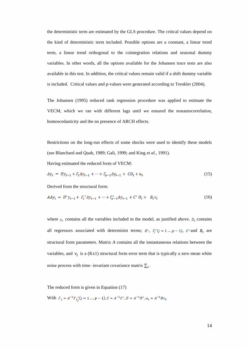
is included. Critical values and p-values were generated according to Trenkler (2004).

The Johansen (1995) reduced rank regression procedure was applied to estimate the

VECM, which we ran with different lags until we ensured the nonautocorrelation,

homoscedasticity and the no presence of ARCH effects.

Restrictions on the long-run effects of some shocks were used to identify these models

(see Blanchard and Quah, 1989; Gali, 1999; and King et al., 1991).

Having estimated the reduced form of VECM:

(15)

Derived from the structural form:

(16)

where contains all the variables included in the model, as justified above. contains

all regressors associated with determinist terms; , , and are

structural form parameters. Matrix A contains all the instantaneous relations between the

variables, and tv is a (Kx1) structural form error term that is typically a zero mean white

noise process with time- invariant covariance matrix

The reduced form is given in Equation (17)

With .

15

It has the following moving-average (MA) representation:

is an infinite order polynomial in the lag operator with a coefficient matrix that goes to

zero as j goes to infinity. The matrix has rank K–r if the cointegrating rank of the

system is r and it represents the long-run effects of forecast error impulse responses,

while represents transitory effects. The term contains all initial values. As the

forecast error impulse responses based on

and are subject to the same criticism as

those for stable VAR processes, appropriate shocks have to be identified for a meaningful

impulse response analysis. If is replaced by , the orthogonalized short-run

impulse responses may be obtained as in a way that is analogous to the stationary

vector autoregressive (VAR) case. Moreover, the long-run effects of shocks are given

by (18).

This matrix has rank K − r because rk( ) = K − r and A and B are non singular. Thus, the

matrix (18) can have at most r columns of zeros. Hence, there can be at most r shocks

with transitory effects (zero long-run impact), and at least k* = K − r shocks have

permanent effects. Given the reduced rank of the matrix, each column of zeros stands for

only k*independent restrictions. Thus, if there are r transitory shocks, the corresponding

zeros represent k*r independent restrictions only. To identify the permanent shocks

exactly we need k*(k* − 1)/2 additional restrictions. Similarly, r (r − 1)/2 additional

contemporaneous restrictions identify the transitory shocks. Together these constitute a

16

total of k*r + k*(k* − 1)/2 + r (r − 1)/2= K(K−1)/2 restrictions21. If we assume that A= ,

the matrix (18) become ΞB, and we have enough restrictions to identify B with the long-

run restrictions explained above.

VI. Empirical results and discussion.

The results of the standard ADF test and the unit root test with a level shift proposed by

Saikkonen and Lütkepohl (2002) and Lanne et al. (2002) for those variables with

structural breaks (presented in Tables 1 and 2 in Appendix C) indicate that the series in

level terms display a unit root and in difference terms (denoted by d1) are stationary22.

The graphics show the presence of structural breaks in the following variables: inflation

(d1_cpi), real effective exchange rate (reer) and oil prices (oil). Since inflation and the

real effective exchange rate variables are highly correlated, both present the same break

date: 2001:M2, while for oil prices the break date is 2009:M1.

The results of the Saikkonen and Lütkepohl cointegration test (2000a)23, presented in

Table 3 in Appendix C, suggest that all variables cointegrate through one cointegration

relation24.

The Johansen (1995) reduced rank estimation procedure was applied in estimating the

VEC model, which has five lags for variables in difference and just one lag for the

21 See Breitung, J., Brüggemann, R. and Lütkepohl, H. (2004). 22The econometric analysis was implemented using JmulTi 4 software (www.jmulti.de). 23If we had not obtained cointegration without the inclusion of dummies so as to take the structural breaks into account,

then we would have included them, but it proved unnecessary because the structural breaks coincided in more than one

variable. It is supposed that the cointegration relation absorbed these structural breaks. See Juselius, 2007. 21We reach the same conclusion with the Johansen Trace test (Johansen, Mosconi and Nielsen, 2000). In the test we specified 1 lag for the variables in levels, two level shifts (2001:M2 and 2009:M1) unrestricted in the model, but seasonal dummies, intercept and trend restricted in the model. We estimate our VECM with the Johansen reduced rank, keeping this structure.

17

cointegrated vector, ensuring the nonautocorrelation, homoscedasticity and the no

presence of ARCH effects.

Even when structural breaks were absorbed in the cointegration space, two dummy

variables had to be included in order to obtain the normality of residues. The first impulse

dummy (dummy01) accounts for the new dollarization period that Ecuador entered in

2001, when its nominal variables seemed to be stable. This was 1 for 2001:M2 and -1 for

2001:M3, reflecting the differentiation of a permanent impulse detected in 2001:M2 by

prior unit root tests. The second dummy (dummy09) takes into account the sudden

decrease in oil prices, which in terms of Ecuadorian money supply took place in

2008:M12. This structural break was detected in prior unit root tests as a level shift in the

oil variable. Following Juselius’ (2007) technique when using dummies in VEC models,

as mentioned above, a shift dummy becomes a permanent dummy when the former is

differentiated, i.e. dummy09 will be -1 in 2009:M1.

By examining the significant loading coefficients ( ) resulting from the VEC estimation

(see Table 4 in Appendix C) through their t-values (based on OLS standard errors), it can

be seen that each significant corresponds to a normalized eigenvector ( ) with the

opposite sign. When this occurs, then the cointegration relation is equilibrium correcting

in the equation Δ . Here we can see that the oil variable is the only one not adjusted with

the long-run inflation relation. This result was expected since this variable does not

depend on domestic variables.

In order to obtain the impulse response function and the variance decomposition of

inflation variable we have to estimate a structural VEC using the long-run restrictions

explained above. Since we have just one cointegration vector, we have r = 1. Hence, there

can be at most one shock with transitory effects (zero long-run impact), and at least three

(k* = 4 – 1) shocks should have permanent effects. Given the reduced rank of the matrix,

18

each column of zeros stands for only k* independent restrictions. Thus, if there is one

transitory shock, the corresponding zeros represent three (k*r) independent restrictions.

To identify the permanent shocks exactly we need three (k*(k* − 1)/2) additional

restrictions. Since r (r − 1)/2 is zero, we do not need additional contemporaneous

restrictions to identify the transitory shocks. Together these constitute a total of six

(K(K−1)/2) restrictions.

With the vector of structural shocks given by the

contemporaneous impact matrix and the identified long run impact matrix , would

have the following restrictions:

B = * * * * = 0 * * *

* * 0 * 0 * * *

* * * * 0 * * *

* * * * 0 0 0 *

The cointegration analysis suggested that inflation is stationary, accordingly inflation has

no long-run impact on the rest of the variables included in the model, which corresponds

to four zero restrictions in the first column of the identified long-run impact matrix. To

derive the rest of the restrictions we employ the theoretical model described in Section 4.

If in the long run the output is supply determined, this restriction is imposed by setting

the elements equal to zero. We are interested in the long-run relation

between money supply and inflation, even in a country which has lost control over its

monetary policy; consequently, as we need one more restriction to identify the parameters

in B, we decided to impose one contemporaneous restriction, that is, , assuming

that money supply does not affect the real effective exchange rate in the short run. This is

a coherent approach as we are analyzing a country with a fixed exchange rate regime in

which the authorities cannot call on international reserves to control it.

19

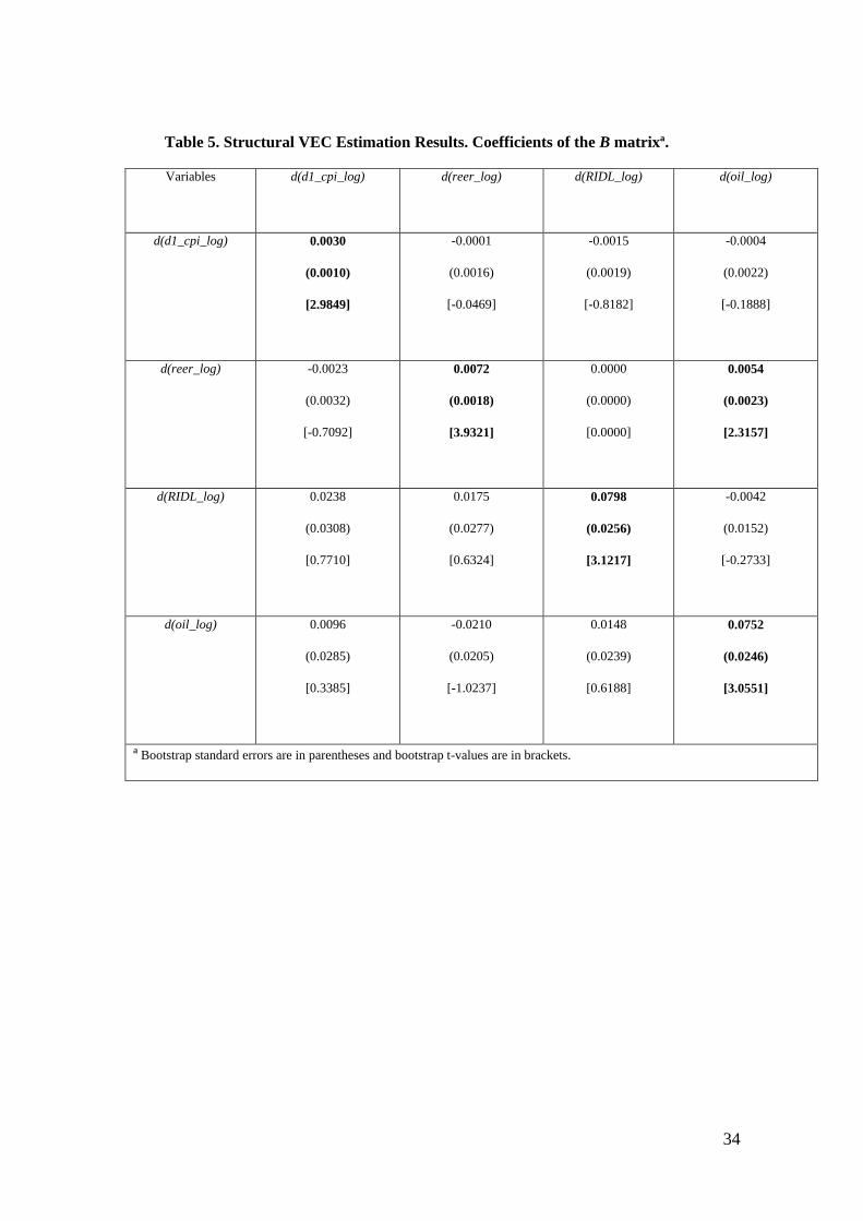
The bootstrapped t-values summarized in Table 5 in Appendix C, obtained using 2,000

bootstrap replications, suggest that only real effective exchange rate shocks significantly

increase inflation in the long run in Ecuador. In the short run only oil price shocks

significantly increase the real effective exchange rate. Both results are consistent with the

assumption that the real effective exchange rate involves both demand and foreign price

shocks. Money supply does not affect inflation significantly in Ecuador, which is to be

expected in a country that cannot use its monetary policy to affect prices, even when this

variable is adjusted to the same long-run relation as the rest of the domestic variables

(d1_cpi, reer). The oil variable is only affected by its own shocks in the short run.

While a pegged exchange rate regime serves to lower inflation in Ecuador, the rest of the

world is experiencing higher rates of inflation. Thus, international currencies are

appreciating in the long run, and rising oil prices exacerbate the effect by pushing

inflation up in oil importing countries (Ecuador’s foreign exporters). The impulse

response graphs (Figure 6 in Appendix C) and the variance decomposition table (Table 6

in Appendix C) illustrate these results: real effective exchange rate depreciations

increased inflation for about twenty periods with a maximal response after two years.

Indeed, the graphs of the variables in Appendix C forecast these conclusions: the real

effective exchange rate follows oil price trends, after dollarization, the real effective

exchange rate fell reaching a low in 2003:M5. After that date the trend reversed,

increasing until the two downturns in oil prices in 2009:M1 and 2010:M7.

VII. Conclusions

In this article we have examined the impact of Ecuador’s real effective exchange rate

depreciations on domestic inflation rates in the period from January 2000 (when Ecuador

officially adopted the US dollar as its domestic currency) to July 2011 (latest available

20

data). We have drawn on the exchange rate pass-through literature and a structural

VECM with long-run restrictions in undertaking the theoretical and empirical analyses.

Although few ERPT studies have specifically examined dollarized countries, Akofio-

Sowah (2008) reports that officially dollarized countries, such as Ecuador, experience a

significantly lower ERPT coefficient. However, the findings reported herein contradict

this. With the estimation of the structural VECM, we obtain the impulse responses of

inflation to a real effective exchange rate shock – these impulse responses can be

interpreted as the trend presented by the exchange rate pass-through. As we have shown,

the real effective exchange rate presents an upward trend, following the trend in oil

prices. As an oil exporter, the higher Ecuadorian oil prices rise, the higher is the inflation

suffered by oil importing countries. These countries are at the same time Ecuador’s

trading partners and so Ecuador imports the inflation of its main trading partners through

these currency appreciations.

Today, the United States remains Ecuador’s principal trading partner, but as emerging

countries such as South Korea and Brazil increase their participation in Ecuadorian trade,

the currencies of such countries can be expected to acquire greater importance than the

US dollar in the Ecuadorian balance sheet: the higher the real effective exchange rate

rises, the greater the inflationary pressures attributable to the higher pass-through in

Ecuador. We believe the inflationary effect reported here would have been even more

marked if we had included China in our real effective exchange rate calculations, given

that China is the emerging country par excellence. However, owing to its relatively new

flexible exchange rate regime, we resolved to postpone its study to a later date.

In our opinion, Ecuador needs to face its short-term economic future with caution since

both banking and currency crises are harmful to the country’s real and nominal variables.

In light of the results, we honestly think that Ecuador is currently missing the

opportunities afforded by managing its own currency and, most significantly, the

21

opportunity of implementing its own monetary policy to manage the shocks it is

experiencing.

References

Akofio-Sowah, N. A. (2009) Is There a Link Between Exchange Rate Pass-Through and

the Monetary Regime: Evidence from Sub-Saharan Africa and Latin America,

International Advance Economic Research, 15, 296–309.

Alesina, A. and Robert, J. Barro (2001) Dollarization, The American Economic Review,

92, 381-385.

Alvarez, R., Jaramillo, P. and Selaive, J. (2008) Exchange rate pass-through into import

prices: the case of Chile, Central Bank of Chile Working Papers No. 465.

Amisano, G. and Giannini, C. (1997) Topics in structural VAR econometrics, 2nd edn,

Springer, Berlin and New York.

An, L. (2006) Exchange Rate Pass-Through: Evidence Based on Vector Autoregression

with Sign Restrictions, Discussion Paper No. 527, MPRA.

Bacchetta, P. and Eric van Wincoop. (2005) A Theory of the Currency Denomination of

International Trade, Journal of International Economics, 67, 295-319.

Barhoumi, K. (2005) Exchange rate pass-through into import prices in developing

countries: an empirical investigation, Economics Bulletin, 3, 1-14.

Barhoumi, K. (2007) Exchange rate pass-through and structural macroeconomic shocks

in developing countries: an empirical investigation, Discussion Paper No. 6573, MPRA.

Barhoumi, K, and Jouini, J. (2008) Revisiting the Decline in the Exchange Rate Pass-

Through: Further Evidence from Developing Countries, Economics Bulletin, 3, 1-10.

Bastourre, Carrera, Feliz and Panigo (2003) Dollarization and real volatility,

CEPREMAP Working Papers in Economics No. 311. Available at

http://www.cepremap.cnrs.fr.

Beckerman, P. and Solimano, A. (2002) Crisis and Dollarization in Ecuador. Stability,

growth and social equity, Directions in Development Series, The World Bank,

Washington, D.C.

Berg. A and Borensztein, E. (2000) The Pros and Cons of full dollarization, IMF

Working Paper No. 00/50.

Bhundia, A. (2002) An empirical investigation of exchange rate pass-through in South

Africa, IMF Working Paper No. 02/165.

Blanchard, O. and Quah, D. (1989) The Dynamic Effects of Aggregate Demand and

Supply Disturbances, American Economic Review, 79, 665-673.

22

Breitung, J., Brüggemann, R. and Lütkepohl, H. (2004) Structural vector autoregressive

modelling and impulse responses, in Applied Time Series Econometrics, 1st edn (Eds)

H. Lütkepohl and M. Krätzig, Cambridge University Press, Cambridge, pp. 159-196.

Campa, J. M. and Goldberg, L. S. (2002) Exchange Rate Pass-Through into Import

Prices: A Macro or Micro Phenomenon?, Federal Reserve Bank of New York, Staff

Report No. 149.

Campa, J. M., Goldberg, L., and González-Mínguez, J. (2005) Exchange Rate Pass-

Through to Import Prices in the Euro Area, NBER Working Paper No. 11632.

Carranza, L., Galdon Sanchez, E. and Gomez Biscarri, J. (2009) Exchange rate and

inflation dynamics in dollarized economies, Journal of Development Economics. 89, 98-

108.

Corden W.M. and Neary J.P., (1982) Booming Sector and De-industrialisation in a Small

Open Economy, The Economic Journal, 92, 829-831.

Coulibaly, D. and Kempf, H. (2010) Does inflation targeting decrease exchange rate pass-

through in emerging countries?, Banque de France Working Papers No. 303.

De Nicoló, G., Honohan, P. and Ize, A. (2005) Dollarization of bank deposits: Causes and

consequences, Journal of Banking & Finance, 29, 1697–1727.

Devereux, M., Engel, C. and Storgaard, P. (2004) Endogenous Exchange Rate Pass-

through when nominal prices are set in advance, Journal of International Economics, 63,

263-291.

Dickey, D. A. and Fuller, W. A. (1979) Estimators for autoregressive time series with a

unit root, Journal of the American Statistical Association, 74, 427-431.

Dornbusch, R. (1987) Exchange Rates and Prices, American Economic Review, 77, 93-

106.

Dornbusch, R. (1985), Purchasing Power Parity, NBER Working Papers No. 1591.

Einchengreen, B. and Hausmann, R. (1999) Exchange rates and financial fragility, NBER

Working Papers No. 7418.

Frankel, J. (2005) Contractionary Currency Crashes In Developing Countries, NBER

Working Papers No. 11508.

Froot, K. A. and Klemperer, P. (1988) Exchange rate pass-through when market share

matters, NBER Working Papers No. 2542.

Gali, J. (1999) Technology, employment, and the business cycle: Do technology shocks

explain aggregate fluctuations?, American Economic Review, 89, 249–271.

Goldberg, P. and Knetter, M. (1997) Goods prices and exchange rates: what have we

learned?, Journal of Economic Literature 35, 1243-1272.

Goldfajn, I. and Werlang, Sergio R.C. (2000) The Pass-through from Depreciation to

Inflation: A Panel Study, Banco Central Do Brasil Working Papers No. 5.

23

Gonzalez Anaya, J. A. (2000) Exchange Rate Pass-through and Partial Dollarization: Is

there a Link?, Center for Research on Economic Development and Policy Reform

Working Papers No. 81.

Hwang, Jen-Te; Wu, Ming-Jia (2011) Inflation and Economic Growth in China: An

Empirical Analysis, China and World Economy, 19, 67-84.

Issing, O. (2011) The crisis of European Monetary Union – Lessons to be drawn, Journal

of Policy Modeling, 33, 737 – 749.

Ito, T. and Sato, K. (2008) Exchange Rate Changes and Inflation in Post-Crisis Asian

Economies: Vector Autoregression Analysis of the Exchange Rate Pass-Through, Journal

of Money, Credit and Banking, 40, 1407–1438.

Jacome, L. (2004) The late 1990s financial crisis in Ecuador: institutional weaknesses,

fiscal rigidities, and financial dollarization at work, IMF Working Papers No. 04/12.

Johansen, S., Mosconi, R. and Nielsen, B. (2000) Cointegration analysis in the presence

of structural breaks in the deterministic trend, Econometrics Journal, 3, 216-249.

Johansen, S. (1995) Likelihood-based Inference in Cointegrated Vector Autoregressive

Models, 1st edn, Oxford University Press, Oxford.

Juselius, K (2006) The Cointegrated VAR Model: Methodology and Applications, 1st edn,

Oxford University Press, USA.

King, G, Plosser, I, Stock, H and Watson, W. (1991) Stochastic Trends and Economic

Fluctuations, American Economic Review, 81, 819-840.

Lanne, M., Lütkepohl, H. (2002). Unit root tests for time series with level shifts: a

comparison of different proposals. Economics Letters 75(1): 109–114.

Lanne, M., Lütkepohl, H. and Saikkonen, P. (2002) Comparison of unit root tests for time

series with level shifts, Journal of Time Series Analysis, 23, 667-685.

Lanne, M., Lütkepohl, H. and Saikkonen, P. (2003) Test procedures for unit roots in time

series with level shifts at unknown time, Oxford Bulletin of Economics and Statistics, 65,

91-115.

Lütkepohl, H. (2004) Univariate time series analysis in Applied Time Series

Econometrics, 1st edn (Eds) H. Lütkepohl and M. Krätzig, Cambridge University Press,

Cambridge, pp. 8-85.

Ma, H. (1998) Inflation, uncertainty and growth in Colombia, IMF Working Papers No.

98/161.

Mann, C.L. (1986) Prices, Profit Margins and Exchange Rates, Federal Reserve Bulletin,

72, 366-379.

McCarthy, J. (2000) Pass-through of exchange rates and import prices to domestic

inflation in some industrialized economies, Federal Reserve Bank of New York Staff

Report No. 111.

Obstfeld, M. (1985), Cooper, R. and Krugman, P. (1985) Floating Exchange Rates:

Experience and Prospects, Brookings Papers on Economic Activity, 2, 369-464.

24

Obstfeld, M. (2000) International Macroeconomics: Beyond the Mundell-Fleming Model,

IMF Staff Papers, Vol. 47.

Reinhart, C., Rogoff, K. and Savastano, M. (2003) Addicted to dollars, NBER Working

Papers No. 10015.

Reinhart, C and Rogoff, K. (2004) The Modern History of Exchange Rate Arrangements:

A Reinterpretation, Quarterly Journal of Economics, 119, 1-48.

Rodriguez, F. (1999) Metodología de cálculo de los índices de tipo de cambio real del

Ecuador, Cuaderno de Trabajo No. 119. Available at

http://www.bce.fin.ec/frame.php?CNT=ARB0000006.

Rowland, P. (2004) Exchange Rate Pass-Through to Domestic Prices: the Case of

Colombia, Revista ESPE, 47, 106-125.

Saikkonen, P. and Lütkepohl, H. (2000a) Testing for the cointegrating rank of a VAR

process with an intercept, Econometric Theory, 16, 373-406.

Saikkonen, P. and Lütkepohl, H. (2000b) Testing for the cointegrating rank of a VAR

process with structural shifts, Journal of Business & Economic Statistics, 18, 451-464.

Saikkonen, P. and Lütkepohl, H. (2000c) Trend adjustment prior to testing for the

cointegrating rank of a vector autoregressive process, Journal of Time Series Analysis, 21,

435-456.

Saikkonen, P. and Lütkepohl, H. ( 2002) Testing for a unit root in a time series with a

level shift at unknown time, Econometric Theory, 18, 313-348.

Shambaugh, J. (2008) A New Look at Pass-through, Journal of International Money and

Finance, 27, 560-591.

Taylor, J. B. (2000) Low Inflation, Pass-Through, and the Pricing Power of Firms,

European Economic Review, 44, 1389-1408.

Trenkler, C. (2004) Determining p-values for systems cointegration tests with a prior

adjustment for deterministic terms, Center for Applied Statistics and Economics (CASE)

Working Papers No. 37, Humboldt-Universitätzu Berlin.

Wilson, Bradley Kemp (2006) The Links between Inflation, Inflation Uncertainty and

Output Growth: New Time Series Evidence from Japan, Journal of Macroeconomics, 28,

609-620.

25

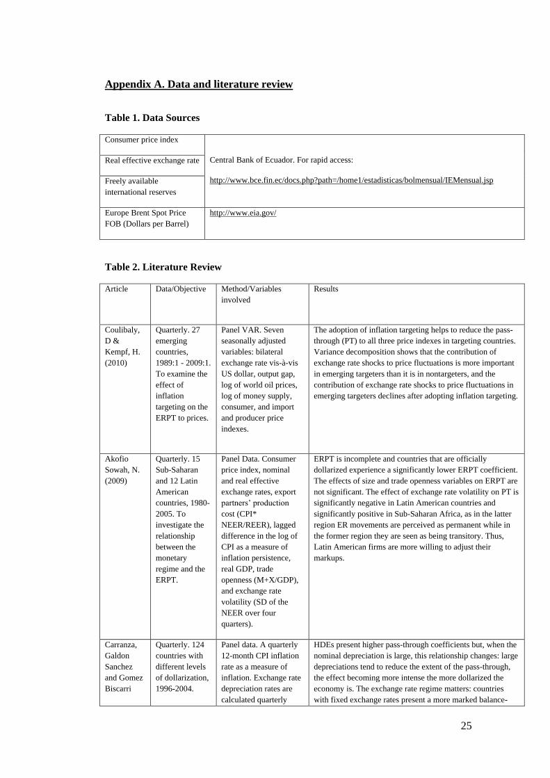
Appendix A. Data and literature review

Table 1. Data Sources

Consumer price index

Central Bank of Ecuador. For rapid access:

http://www.bce.fin.ec/docs.php?path=/home1/estadisticas/bolmensual/IEMensual.jsp

Real effective exchange rate

Freely available

international reserves

Europe Brent Spot Price

FOB (Dollars per Barrel)

http://www.eia.gov/

Table 2. Literature Review

Article

Data/Objective Method/Variables

involved

Results

Coulibaly,

D &

Kempf, H.

(2010)

Quarterly. 27

emerging

countries,

1989:1 - 2009:1.

To examine the

effect of

inflation

targeting on the

ERPT to prices.

Panel VAR. Seven

seasonally adjusted

variables: bilateral

exchange rate vis-à-vis

US dollar, output gap,

log of world oil prices,

log of money supply,

consumer, and import

and producer price

indexes.

The adoption of inflation targeting helps to reduce the pass-

through (PT) to all three price indexes in targeting countries.

Variance decomposition shows that the contribution of

exchange rate shocks to price fluctuations is more important

in emerging targeters than it is in nontargeters, and the

contribution of exchange rate shocks to price fluctuations in

emerging targeters declines after adopting inflation targeting.

Akofio

Sowah, N.

(2009)

Quarterly. 15

Sub-Saharan

and 12 Latin

American

countries, 1980-

2005. To

investigate the

relationship

between the

monetary

regime and the

ERPT.

Panel Data. Consumer

price index, nominal

and real effective

exchange rates, export

partners’ production

cost (CPI*

NEER/REER), lagged

difference in the log of

CPI as a measure of

inflation persistence,

real GDP, trade

openness (M+X/GDP),

and exchange rate

volatility (SD of the

NEER over four

quarters).

ERPT is incomplete and countries that are officially

dollarized experience a significantly lower ERPT coefficient.

The effects of size and trade openness variables on ERPT are

not significant. The effect of exchange rate volatility on PT is

significantly negative in Latin American countries and

significantly positive in Sub-Saharan Africa, as in the latter

region ER movements are perceived as permanent while in

the former region they are seen as being transitory. Thus,

Latin American firms are more willing to adjust their

markups.

Carranza,

Galdon

Sanchez

and Gomez

Biscarri

Quarterly. 124

countries with

different levels

of dollarization,

1996-2004.

Panel data. A quarterly

12-month CPI inflation

rate as a measure of

inflation. Exchange rate

depreciation rates are

calculated quarterly

HDEs present higher pass-through coefficients but, when the

nominal depreciation is large, this relationship changes: large

depreciations tend to reduce the extent of the pass-through,

the effect becoming more intense the more dollarized the

economy is. The exchange rate regime matters: countries

with fixed exchange rates present a more marked balance-

26

(2009)

To provide an

in-depth

analysis of the

pass through

from exchange

rate changes

into inflation by

taking into

account the

likely balance-

sheet effect

present in

highly

dollarized

economies

(HDE)

using the nominal

exchange rate expressed

in units of local

currency per dollar. The

ratio of exports plus

imports to GDP to

measure the openness of

a country. Real GDP

growth to control the

business cycle. Real

Gross Fixed Capital

Formation growth

(GFCF). Two dummies

that control for fixed

and intermediate

regimes.

sheet effect, whereas the evidence for intermediate regimes is

weaker and countries with flexible regimes do not seem to

experience the balance-sheet effect at all. A contraction in

investment may indeed be the mechanism that generates the

reduction in inflation pass-through. Openness appears

positively related to the intensity of pass-through. The

inclusion of GDP growth has an interesting effect: fast

growing countries show smaller inflation pass-through.

Alvarez,

Jaramillo

and Selaive

(2008)

Monthly 1996-

2007.

To estimate a

pass-through

into

disaggregated

import data in

Chile.

Single equation model.

Nominal effective

exchange rate, but with

the NEER expressed as

US dollar parity they

obtained similar results.

As a proxy for foreign

prices: external price

index. Commodities

price index (minus fuel)

to control for changes in

import prices. Monthly

index of economic

activity. Seasonally

adjusted. Dummy

variables to test if PT is

asymmetric

In Chile the PT is high. The evidence of asymmetric PT for

the aggregate import indexes is weak and none is found to

indicate that the high PT is attributable to the concentration

of Chilean imports in products with high ERPT. Yet

regressions suggest heterogeneity in ERPT for individual

products.

Ito, T. and

Sato, K.

(2008)

Monthly from

1994-2006. To

examine pass-

through effects

of exchange rate

changes on

domestic prices

in East Asian

countries.

VAR. Five variables:

CPI, producer (PPI) and

import price index (IPI),

log of oil prices, output

gap, log of money

supply, nominal

effective exchange rate.

All prices and industrial

production index are

adjusted seasonally.

Another VAR including

interest rates.

The pass-through effect is greatest on IPI, followed by that

on PPI, and is smallest on CPI. The degree of price response

to the exchange rate shock is greatest in Indonesia being

most pronounced in its CPI. Only Indonesia presents

positive, large and statistically significant impulse responses

of its monetary base to the NEER shock and of its CPI to the

monetary shock. Indonesia’s disappointing recovery after the

crisis can be partly attributed to the large pass-through of

exchange rate shocks to CPI, the breakdown in its domestic

distribution networks, and the central bank’s monetary policy

reaction to depreciation.

Barhoumi,

K. (2007)

Quarterly. 12

developing

countries.

1980:1 - 2001:4.

To calculate PT

as the responses

of ER, CPI and

Structural VECM and

the common trends

approach. All five

variables in logs.

Proxies of GDP:

industrial production,

petroleum production,

Adopts a new formulation to show that PT to both CPI and

import prices are in general greater than one, indicating that

developing countries face larger shocks. ERPT is higher in

the higher inflation environments of developing countries,

showing that inflation is an important determinant of such

countries’ PT.

27

import prices to

the supply, the

relative demand,

the nominal and

the foreign

prices shocks.

manufacturing

production. Nominal

and real effective

exchange rate.

Consumer price index,

import unit values.

Demand shocks raise both domestic and import prices, and

depreciate nominal exchange rate. Supply shocks lower both

domestic and import prices and appreciate nominal exchange

rate. Nominal shocks increase all nominal variables. Foreign

shocks raise both domestic and import prices. CPI rises

higher than import prices.

Shambaugh

J. (2008)

Quarterly. 16

countries,

developed and

developing.

Data from 1973-

1994. To

identify shocks

and explore the

way domestic

prices, import

prices and

exchange rates

react to these

shocks.

Long-run restrictions

VAR. Variables in logs:

industrial production as

proxy of GDP, nominal

and real exchange rates

series are based on

relative CPI, import

prices (y, q, p, s and

pm)

Supply shocks lower prices, appreciate nominal rates and

lower import prices. Demand shocks have a positive impact

on output in the short run, depreciate the real exchange rate,

raise domestic prices a small amount but raise import prices

permanently. Nominal shocks have a positive impact on

industrial production, depreciate the nominal exchange rate

and increase all the nominal variables. Foreign shocks

depreciate nominal exchange rates. However, supply and

nominal shocks are much larger in developing countries,

while the effect of a demand shock is somewhat weaker in

industrialized countries.

Barhoumi,

K. and

Jouini, J.

(2008)

Quarterly. Eight

developing

countries.

1980:2 - 2003:4.

To revisit the

Taylor (2000)

proposition.

Structural change and

cointegration tests

suitable for the single

equation case. Five

variables in logs:

Percentage change of

CPI. Nominal and real

effective exchange rates.

Industrial price index

and import unit value.

During the 1990s some developing countries experienced a

significant fall in inflation induced by a shift in their

monetary policy regimes that specifically targeted inflation.

Barhoumi,

K (2005)

Annual. 24

developing

countries. 1980-

2003.

To define and

estimate ERPT.

Nonstationary panel

techniques. Four

variables in logs:

nominal effective

exchange rate,

wholesale price index,

producer price index,

GDP, import unit value

in domestic currency.

The long-run exchange rate pass-through is heterogeneous,

depending on local monetary policy and country size. The

long-run ERPT is determined by a combination of the

nominal effective exchange rate, the price of the competing

domestic products, the exporter’s cost and domestic demand

conditions.

Rowland,

P. (2004)

Monthly. 20

years of data

from 1983-

2002. To study

ERPT to import,

UVAR using the

Johansen framework.

Variables in logs and

seasonally adjusted:

nominal bilateral

Import prices respond rapidly to an exchange rate shock.

Producer and consumer prices respond much more

sluggishly.

28

producer and

consumer prices

in Colombia.

USD/COP rate of

exchange (because the

trade weighted nominal

effective exchange rate

residuals did not pass

the test of normality.

Besides, the US is by far

Colombia’s largest

trading partner and a

large majority of

exports and imports are

priced in US dollars),

and all prices from the

distribution chain.

Carranza,

Galdon

Sanchez

and Gomez

Biscarri

(2004)

Monthly. 15

countries with

different

degrees of

dollarization.

1991-2003.

OLS to time series. As a

measure of inflation 12-

month CPI inflation

rate, nominal exchange

rate vis-à-vis the dollar

and an indicator of

recessionary periods

(Rc).

Pass-through is significantly higher in dollarized countries.

The asymmetry in the pass-through depends on the economic

cycle: the PT during recessions tends to be negative (the

more markedly so, the higher the degree of dollarization in

the economy), because the drop in the aggregate demand

prevents domestic prices rising.

Reinhart,

C., Rogoff,

K. and

Savastano,

M. (2003)

Annual: two

samples: 89

countries from

1996-2001.

Panel data. CPI, real

exchange rate, GDP and

proxies to control for

the openness of country

and other variables such

as seigniorage and the

level of dollarization of

each country.

The exchange rate pass-through to prices was greatest in

economies where the degree of dollarization was very high,

suggesting a link between “fear of floating” and the degree of

dollarization: countries tend to be less tolerant to large

exchange rate changes out of concern for the adverse effects

such changes may have on sectoral balance sheets and,

ultimately, on aggregate output.

Bhundia, A.

(2002)

Quarterly from

1980-2001.

To analyze the

ERPT, to

distinguish

between real

and nominal

shocks and to

investigate their

impact on the

exchange rate

and prices.

South Africa

VAR with long run

restrictions. Six

variables based on

McCarthy (1999): oil

prices, output gap,

nominal effective

exchange rate (the

results using the

bilateral exchange

rand/US dollar are

similar), import prices,

producer prices and

CPI. A dummy variable

to control for the change

in 1994 with the post

apartheid government

Shocks to producer prices have a considerable impact on

CPI. When real shocks are responsible for nominal exchange

rate depreciation the response of inflation is much smaller.

Gonzalez

Anaya,

J.A.. (2000)

Monthly. Data

from 1980-

2000. 16

Error Correction Model

and Panel Data.

Nominal dollar

There is no significant cross-country or within-country

correlation between dollarization and pass-through.

29

dollarized

countries of

Latin America

exchange rate. CPI, US

PPI, G7 PPI as

international prices. M4.

Goldfajn, I

and

Werlang, S.

(2000)

71 countries

from 1980-1998

Panel Data. GDP gap,

accumulated inflation

calculated as the

difference between CPI

index at t+12 and t,

proxy for trade

openness, depreciation

as changes in effective

nominal exchange rate,

and a proxy to capture

the misalignment of the

real exchange rate.

The PT coefficient increase as the time horizon of the

regression is expanded. American and Asian regions have a

higher ERPT to prices than that of the other regions. The

economically significant determinants are the degree of ER

overvaluation and initial inflation.

30

Appendix B Figures

Fig. 1 Chinese Yuan Renminbi exchange rates against US dollar (Monthly Average)

8,2700

6,3548

0

1

2

3

4

5

6

7

8

9

10

Jan

-90

Jun

-90

No

v-90

Ap

r-91

Sep

-91

Feb

-92

Jul-

92

Dec

-92

May

-93

Oct

-93

Mar

-94

Au

g-94

Jan

-95

Jun

-95

No

v-95

Ap

r-96

Sep

-96

Feb

-97

Jul-

97D

ec-9

7M

ay-9

8

Oct

-98

Mar

-99

Au

g-99

Jan

-00

Jun

-00

No

v-00

Ap

r-01

Sep

-01

Feb

-02

Jul-

02

Dec

-02

May

-03

Oct

-03

Mar

-04

Au

g-04

Jan

-05

Jun

-05

No

v-05

Ap

r-06

Sep

-06

Feb

-07

Jul-

07D

ec-0

7M

ay-0

8

Oct

-08

Mar

-09

Au

g-09

Jan

-10

Jun

-10

No

v-10

Ap

r-11

Sep

-11

Source: http://fxtop.com. Notes: Fig. 1 shows the appreciation of CNY/USD since China reformed its fixed exchange rate regime to a

managed floating exchange rate system in July 2005.

Fig. 2. Evolution of both the Colombian Peso and Yen exchange rates against the US dollar

(Monthly average)

0

20

40

60

80

100

120

140

160

may

-00

ago

-00

no

v-00

feb

-01

may

-01

ago

-01

no

v-01

feb

-02

may

-02

ago

-02

no

v-02

feb

-03

may

-03

ago

-03

no

v-03

feb

-04

may

-04

ago

-04

no

v-04

feb

-05

may

-05

ago

-05

no

v-05

feb

-06

may

-06

ago

-06

no

v-06

feb

-07

may

-07

ago

-07

no

v-07

feb

-08

may

-08

ago

-08

no

v-08

feb

-09

may

-09

ago

-09

no

v-09

feb

-10

may

-10

ago

-10

no

v-10

feb

-11

may

-11

ago

-11

no

v-11

0

500

1000

1500

2000

2500

3000

3500

JPY/USD

COP/USD

Source: http://fxtop.com

Notes: Fig. 2 shows the appreciation of two currencies belonging to two of Ecuador’s main trading partner

Colombia and Japan.

31

0,0

1.000,0

2.000,0

3.000,0

4.000,0

5.000,0

6.000,0

7.000,0

8.000,0

1998 1999 2000 2001 2002 2003 2004 2005 2006 2007 2008 2009 2010

Fig. 3 Ecuador imports CIF by region ($US Millions)

United States Latino American Integration Association Andean Community Europe Asia Africa

Source: Based on statistics provided by the Central Bank of Ecuador.

Notes: Fig. 3 shows the evolution in Ecuador’s main suppliers: the most important are the United States, the Latin

American Integration Association (Argentina, Brazil, Chile and Mexico) and the Andean Community (Bolivia,

Colombia, Peru and Venezuela). The picture also shows the growth recorded by Asia (comprising Japan, Taiwan,

China and South Korea), which since 2004 has replaced Europe as the third largest source of imports.

32

Appendix C. Econometric analysis

Graphics of the variables in logarithms

Unit root and cointegration tests.

Table 1. Unit root with structural break test (Saikkonen and Lütkepohl, 2002 and

Lanne et al., 2002).

Variable Deterministic terms* Lags Break date Value of

test

statistic

Critical Values (Lanne, 2002)

1% 5% 10%

d1_cpi_log C + Time trend + ID + SD 1 2001M2 -2.2576 -3.55 -3.03 -2.76

d1_cpi_log_d1 ID 0 2001M2 -14.6855 -3.48 -2.88 -2.58

reer_log C + Time trend + Shift D 1 2001M2 0.1508 -3.55 -3.03 -2.76

reer_log_d1 ID 0 2001M2 -5.8671 -3.48 -2.88 -2.58

oil_log C + Time trend + Shift D 1 2008M12 -2.9592 -3.55 -3.03 -2.76

oil_log_d1 ID 0 2009M1 -10.0459 -3.48 -2.88 -2.58

*C: Constant, ID: Impulse dummy, Shift D: Shift dummy, SD: Seasonal Dummies

33

Table 2. ADF Test (Fuller, 1976, Dickey and Fuller, 1979)

Variable Deterministic terms* Lags Value of test

statistic

Critical Values (Davidson and

MacKinnon, 1993)

1% 5% 10%

RIDL_log C + Time trend + SD 0 -2.1764 -3.96 -3.41 -3.13

RIDL_log_d1 C + SD 0 -10.8122 -3.43 -2.86 -2.57

*C: Constant, SD: Seasonal Dummies

Table 3. Cointegration test between d1_cpi, reer, RIDL and oil variables (Saikkonen

& Lütkepohl, 2000).

r0

LR

p value

Critical Values (Trenkler, 2004)

90% 95% 99%

0 85.68 0.0000 42.05 45.32 51.45

1 25.27 0.1234 26.07 28.52 33.50

2 5.25 0.8483 13.88 15.76 19.71

3 0.15 0.9877 5.47 6.79 9.73

Notes: Deterministic terms restricted in the cointegration space: Trend, constant and seasonal dummies.

Optimal Lag: 1 (Hannan-Quinn Criterion and Schwarz Criterion).

Table 4. VECM Estimation Results

Loading coefficientsª Coefficients of the cointegrating vector (ec1(t-1))

d(d1_cpi_log) d(reer_log) d(RIDL_log) d(oil_log) d1_cpi_log(t-1) reer_log (t-1) d(RIDL_log) d(oil_log)

-0.524 0.3 -4.122 -1.671

(0.049) (0.132) (1.209) (1.136)

[-10.789] [2.985] [-3.410] [-1.471]

1.000 -0.089 0.001 0.009

(0.000) (0.012) (0.004) (0.004)

[0.000] [-7.537] [0.242] [2.495]

ª Standard deviations are in parentheses and t-values are in brackets.

34

Table 5. Structural VEC Estimation Results. Coefficients of the B matrixª.

Variables

d(d1_cpi_log) d(reer_log) d(RIDL_log) d(oil_log)

d(d1_cpi_log)

0.0030

(0.0010)

[2.9849]

-0.0001

(0.0016)

[-0.0469]

-0.0015

(0.0019)

[-0.8182]

-0.0004

(0.0022)

[-0.1888]

d(reer_log)

-0.0023

(0.0032)

[-0.7092]

0.0072

(0.0018)

[3.9321]

0.0000

(0.0000)

[0.0000]

0.0054

(0.0023)

[2.3157]

d(RIDL_log)

0.0238

(0.0308)

[0.7710]

0.0175

(0.0277)

[0.6324]

0.0798

(0.0256)

[3.1217]

-0.0042

(0.0152)

[-0.2733]

d(oil_log)

0.0096

(0.0285)

[0.3385]

-0.0210

(0.0205)

[-1.0237]

0.0148

(0.0239)

[0.6188]

0.0752

(0.0246)

[3.0551]

ª Bootstrap standard errors are in parentheses and bootstrap t-values are in brackets.

35

Table 5 (continuation). Coefficients of the long run impact matrix .

Variables d(d1_cpi_log) d(reer_log) d(RIDL_log) d(oil_log)

d(d1_cpi_log)

0.0000

(0.0000)

[0.0000]

0.0024

(0.0011)

[2.1669]

-0.0009

(0.0015)

[-0.5539]

0.0009

(0.0041)

[0.2154]

d(reer_log)

0.0000

(0.0000)

[0.0000]

0.0274

(0.0126)

[2.1803]

-0.0090

(0.0171)

[-0.5252]

0.0197

(0.0561)

[0.3507]

d(RIDL_log)

0.0000

(0.0000)

[0.0000]

0.0038

(0.0224)

[0.1718]

0.0562

(0.0277)

[2.0276]

0.0495

(0.1093)

[0.4526]

d(oil_log)

0.0000

(0.0000)

[0.0000]

0.0000

(0.0000)

[0.0000]

0.0000

(0.0239)

[0.0000]

0.0876

(0.1529)

[0.5728]

Notes: This is a B-model with long-run restrictions. With long-run restrictions providing five independent

restrictions and one contemporaneous restriction providing one additional restriction, the Structural VAR is

just identified. ML Estimation, Scoring Algorithm (see Amisano & Giannini, 1992). Convergence after 11

iterations. Log Likelihood: 1791.3097

36

Fig. 6. Impulse responses

Legend: _____ SVEC Impulse Reponses ------- 95% Hall Percentile (B = 2000, h = 32)

Table 6. SVEC Forecast error variance decomposition of "d1_cpi_log"

Forecast Horizon d1_cpi_log reer_log RIDL_log oil_log

1 0.78 0.00 0.20 0.01

2 0.76 0.00 0.23 0.01

3 0.67 0.08 0.24 0.01

4 0.61 0.14 0.24 0.01

5 0.55 0.20 0.22 0.03

6 0.50 0.27 0.20 0.03

7 0.46 0.31 0.18 0.05

8 0.42 0.37 0.15 0.05

9 0.39 0.41 0.14 0.06

10 0.36 0.44 0.14 0.06

11 0.33 0.47 0.13 0.06

12 0.30 0.50 0.14 0.06

13 0.27 0.53 0.13 0.06

14 0.25 0.55 0.13 0.06

15 0.23 0.57 0.13 0.06

16 0.22 0.59 0.13 0.06

17 0.20 0.61 0.13 0.07

18 0.19 0.62 0.12 0.07

19 0.18 0.63 0.12 0.07

20 0.16 0.64 0.12 0.08