partisan and bipartisan gerrymanderingfmpartisan gerrymandering (order-and-partition).7 we will also...
TRANSCRIPT

Partisan and Bipartisan Gerrymandering∗
Hideo Konishi† Chen-Yu Pan‡
August 4, 2018
Abstract
This paper analyzes the optimal partisan and bipartisan gerryman-dering policies in a model with electoral competitions in policy posi-tions and transfer promises. Party leaders have both office- and policy-motivations. With complete freedom in redistricting, partisan gerry-mandering policy generates the most one-sidedly biased district profile,while bipartisan gerrymandering generates the most polarized districtprofile. In contrast, with limited freedom in gerrymandering, both par-tisan and bipartisan gerrymandering tend to prescribe the same policy.
Keywords: electoral competition, partisan gerrymandering, bipartisangerrymandering, policy convergence/divergence, pork-barrel politics
JEL Classification Numbers: C72, D72
∗We thank Jim Anderson, Emanuele Bracco, Klaus Demset, Mehmet Ekmekci, AlanMiller, Ron Siegel, and participants of PET 2017 in Paris for their comments and sugges-tions.†Corresponding Author: Hideo Konishi: Department of Economics, Boston College,
USA. Email: [email protected]‡Chen-Yu Pan: School of Economics and Management, Wuhan University, PRC. Email:

1 Introduction
It is widely agreed upon that election competitiveness has decreased signifi-cantly in recent decades. For example, the re-election rate of the US House ofRepresentatives has increased from 91.82% in 1950 to 98.25% in 2004 (Fried-man and Holden 2009). Also, 74 House seats were won by a margin of lessthan 55% in 2000, but this number decreased to 24 in 2004 (Fiorina et al.2011). During the same period, Congress has become quite polarized. In the1960s, the distribution of the representatives’ political positions was concen-trated more toward the center of the political spectrum, with considerableoverlap between Republicans’ and Democrats’ positions. By the 2000s, thepositions became sharply twin-peaked with less overlap.1 One popular expla-nation for this phenomenon in US politics is gerrymandering. Fiorina et al.(2011) argue that gerrymandering biased toward incumbents, i.e., bipartisangerrymandering, has an effect on the decrease in competitiveness, since bothparties try to secure their incumbent seats.2 They also suggest that this de-crease in competitiveness may be one of the causes of the recent politicalpolarization in Congress, since proposing more polarized positions does notjeopardize secured seats.3
In contrast, partisan gerrymandering is commonly used to increase thepower of a political party, and it may or may not reduce district competitive-ness, since the party tries to secure their incumbents but at the same time maycreate competitive districts to capture the opposing party’s districts. Recently,there have been many partisan gerrymandering lawsuits against state legisla-tures to request redistricting of state congressional maps, including Pennsyl-
1It is now standard to use a one-dimensional scaling score (DW-Nominate procedureon economic liberal-conservative, Poole and Rosenthal, 1997) to measure representatives’political positions.
2Fiorina et al. (2011) state that “Many (not all) observers believe that the redistrictingthat occurred in 2001-2002 had a good bit to do with this more recent decline in competitiveseats—the party behaved conservatively, concentrating on protecting their seats rather thanattempting to capture those of the opposition.” (see Fiorina et al., pp. 214-215).
3Since polarization has complicated causes, this argument has limitations. Citing thatpolarization has also been happening in the Senate, Fiorina et al. (2011, pp. 219) suggestthat “redistricting is only a minor part of congressional polarization, or that it is importantonly in combination with other factors such as closed primaries.” Alternative explanationsfor polarization include voters’ party sorting and geographical sorting. The former says thatvoters became sorted into Republican and Democratic parties in the latter half of 1900s dueto party elites’ polarization (Levendusky 2009). See also Gilroux (2001). The latter says thatvoters sort themselves into more ideologically homogeneous districts, causing polarization.The rationale behind this is that districts seem to polarize more between redistricting thanduring them (McCarty, Poole, and Rosenthal 2009).
2
vania, Maryland, Wisconsin, and North Carolina.4 In these cases, the courtsrely on a measure of vote misrepresentation, the efficiency gap, and heated de-bates are going on as to whether or not this is an appropriate measure to use(Bernstein and Duchin 2017 and Chambers, Miller, and Sobel 2017).5 Sincethese two methods loom large in US politics and public debates, we go onestep further to see how different the resulting district maps under partisan andbipartisan gerrymandering are, and how polarized the elected representativesare.
In this paper, we will investigate the difference between optimal partisanand bipartisan gerrymandering and the effects on representative policy posi-tions in a unified framework. For this purpose, we introduce party leaders whoare not only office-motivated but also policy-motivated, which is also new tothe literature. We set up a two-party political competition model in whichparty leaders compete with their candidates’ (unidimensional) political po-sitions and pork-barrel promises in each electoral district.6 We assume thatthere are minimum units of indivisible localities with the same population, andthat a gerrymanderer partitions the set of localities freely to create electoraldistricts. Each locality has a voter distribution, and we say that the gerryman-derer has more freedom in redistricting if the distribution is concentrated ona point on the political spectrum. With pork-barrel politics, the party leaderunderstands that pork-barrel policies in competitive districts are costly, andtherefore she has strong incentives to collect her supporters in the winningdistricts in order to avoid large pork-barrel promises.
Traditionally, the literature on gerrymandering often discusses two tacticsin partisan gerrymandering: one is to concentrate or “pack” those who sup-port the opponent in losing districts, and the other is to evenly distribute or“crack” supporters in winning districts. Packing serves to waste the oppos-ing party’s strong supporters’ votes, while cracking utilizes the votes of partysupporters as effectively as possible. Owen and Grofman (1988) show that
4In February 2018, the Pennsylvania Supreme Court blamed the states’ district map onpartisan gerrymandering, and told state lawmakers to redraw the state’s 18 House districts,which currently favor Republicans.
5The efficiency gap and the vote-seat curve are measures based on only two numbers,the vote shares and the seat shares of the two parties, which may not contain sufficientinformation to appropriately evaluate partisan gerrymandering. As Chambers et al. (2017)correctly recognize, the presence of extremists and election uncertainty should be taken intoaccount. For example, consider the outcome of conservative bipartisan gerrymandering. It ispossible that the resulting redistricting plan generates extremely polarized policy positionsfor the elected representatives but is still perfectly desirable under criteria like the efficiencygap or the seat-vote curve.
6We assume that party leaders can choose their candidates’ policy positions freely.
3

a pack-and-crack policy is optimal when a partisan gerrymanderer has lim-ited freedom in redistricting (a constant-average constraint: see the literaturereview). In contrast, Friedman and Holden (2008) argue that advances in com-puting technologies and the availability of big data sets allow gerrymanderershigher degrees of freedom in redistricting, and they obtain a very different op-timal policy from pack-and-crack: the slice-and-mix policy, in which districtsare created by first mixing the strongest opposition group of voters and thestrongest supporter group, then mixing the second strongest opposition andsupporting groups, and so on. This policy wastes opposition groups’ votes,generating the most one-sided allocation from the most extreme to the mostmoderate districts.
Assuming that party leaders are also policy-motivated, we show that theoptimal policies are not the same as the ones in the literature. We showthat the slice-and-mix policy is still optimal for the party leaders in chargeof partisan gerrymandering when they can redistrict with complete freedom.In contrast, when the freedom on gerrymandering is limited by the constraintin redistricting imposed by Owen and Grofman (1988), we obtain a differ-ent result: when voters and party leaders are highly policy-sensitive (roughlyspeaking), a consecutive partition of localities is also the optimal policy forpartisan gerrymandering (order-and-partition).7 We will also systematicallycompare the optimal policies under partisan and bipartisan gerrymanderingwhen the gerrymanderer(s) face different levels of freedom in redistricting. Weshow that when the gerrymanderer can redistrict with complete freedom, theresulting outcomes in partisan and bipartisan gerrymandering are very dif-ferent: bipartisan gerrymandering results in the polarized electoral districtswithout leaving moderate and competitive ones, while partisan gerrymander-ing results in a one-sided allocation, leaving some competitive districts. Incontrast, when the gerrymandering freedom is limited, a consecutive partitionof localities is the optimal order-and-partition policy for both partisan andbipartisan gerrymandering.8
The rest of the paper is organized as follows. Section 2 discusses relatedliterature. In Section 3, we introduce our model and analyze electoral compe-tition in each district. In Section 4, we investigate the optimal gerrymanderingstrategy when the party leader has complete freedom. In Section 5, we proceedto cases where the gerrymanderer’s freedom is limited. Section 6 concludes thestudy. All proofs are collected in Appendix A.
7The optimal policy is different from pack-and-crack in our model, since party leadersare assumed to be policy-motivated, unlike in Owen and Grofman (1988).
8See the the Section 2 for an empirical observation in Friedman and Holden (2009).
4

2 Related Empirical and Theoretical Litera-
ture
Recent empirical studies show that the effects of gerrymandering may be in-conclusive. Friedman and Holden (2009) investigate whether or not the House-incumbent re-election rate depends on gerrymandering being partisan or bi-partisan.9 In partisan gerrymandering cases, the majority party may try tooust the opposing party’s incumbents, and this may be reducing the incumbentre-election rate. In contrast, in bipartisan gerrymandering cases, both partiestry to secure their incumbents’ re-election, maximizing safe seats.10 Interest-ingly, Friedman and Holden (2009) study the data up to 2004 and do notfind significant differences between bipartisan and partisan gerrymanderingeffects on the rising incumbent re-election rate.11 As they mention, this resultsuggests that partisan gerrymandering may not be as effective as popularlythought. In another interesting paper, Grainger (2010) finds that legislativelydrawn districts have been less competitive with more extreme voting positions(polarization) than panel-drawn districts by using a quasi-natural experimentthat alternates between legislatively drawn and panel-drawn districts in Cali-fornia.12 McCarty et al. (2006, 2009) document that the political polarizationof the House of Representatives has increased in recent decades, using data onroll call votes, but they find only a minimal relation between polarization andgerrymandering.13,14
The pioneering paper that laid out the analytical framework of gerryman-dering problems is Owen and Grofman (1988). They introduce uncertaintyin each district’s median voter’s position and consider the situation where a
9Redistricting in the US is usually conducted by state legislatures (partisan gerryman-dering), but in Arizona, Hawaii, Idaho, Montana, New Jersey, and Washington it is con-ducted by bipartisan redistricting commissions. In California and Iowa, redistricting linesare drawn by nonpartisan redistricting committees.
10According to Cain (1985), the goal of bipartisan gerrymanding is to protect incumbentsof both parties, whereas partisan gerrymanding seeks to provide an advantage to one party.
11After 2008, the incumbent re-election rate went down significantly.12Grainger (2010) provides a detailed history of Californian redistricting: in 1970s and
1990s, district lines were drawn by independent panels of judges, whereas in the 1960s,1980s, and 2000s, redistricting was done legislatively. He uses this quasi-natural experimentto test the hypotheses. Interestingly, the 1960s and 2000s redistrictings were bipartisan,whereas those in the 1980s were partisan and led by the Democrats.
13Krasa and Polborn (2015) argue that their answer may be incomplete if the politicalpositions of district candidates are mutually interdependent.
14As early evidence, Ferejohn (1977) finds little support for gerrymandering being thecause of the decline in competitiveness of congressional districts in the 1960s.
5
partisan gerrymanderer redesigns districts in order to maximize the expectednumber of seats in a partisan gerrymandering setup. They assume that theuncertainty in the median voter’s political position is local and independentacross districts when the objective is expected number of seats. Assumingthat the average position of district median voters must stay the same af-ter redistricting (a constant-average constraint), they show that the optimalstrategy is “packing” the opponents in losing districts, and “cracking” the restof voters evenly across the winning districts with substantial margins, so thatthe party can win districts even in cases of negative shocks.15,16 Friedmanand Holden (2008), on the other hand, assume that a partisan gerrymandererhas full freedom in allocating the population over a finite number of districts,and that she maximizes the expected number of seats when there is only va-lence uncertainty in median voters’ utilities (thus, there is no uncertainty inthe median voter’s political position). In this idealized situation, they findthat the optimal strategy is “slice-and-mix,” which is similar to our optimalstrategy under a different model. Thus, theoretically, the levels of freedom ingerrymandering can affect the optimal policy.
In bipartisan gerrymandering, Gul and Pesendorfer (2010) extend Owenand Grofman (1988) by introducing a continuum of districts and voters’ partyaffiliations. Here, bipartisan gerrymandering means that the two parties owntheir territories and redistrict exclusively within each territory. They assumethat each party leader can redistrict her party’s territory (the districts withher party’s seats) independently, maximizing the probability of winning themajority of seats.17 They show that the optimal policy is again a version of“pack-and-crack.” However, these papers do not compare the optimal parti-san and bipartisan gerrymandering policies. They also do not model spatialcompetition in policy positions, and the elected representatives’ positions areimplicitly assumed to be the district median voters’ positions (Downsian com-petition).
Our model is related to vote-buying models like the one in Dekel, Jackson,and Wolinsky (2008), in which the political competition is deterministic and
15They also consider the case where the partisan gerrymanderer maximizes the proba-bility to win a working majority of seats for her party by assuming that the uncertainty isglobal. They again get pack-and-crack policy as the optimal policy.
16The original “cracking” tactics are to create the maximum number of winning districtswith the smallest margins. In the traditional literature, some argue that gerrymandering willincrease political competition for this reason. In this paper, we use the “cracking” tacticsfrom Owen and Grofman (1988).
17They consider two feasibility constraints. The first is the constant mean of medianvoters’ positions which is the same as the one in Owen and Grofman (1988). The second isthat the status quo needs to be a mean-preserved spread of a feasible redistricting plan.
6

modeled as an auction process with a discrete bidding increment. This paperadopts the traditional continuous policy proposal and adds a gerrymanderingstage. Although our model seem to be related to the so-called probabilisticvoting model in, for example, Lindbeck and Weibull (1987) and Dixit andLondregan (1996), the voting decision in our model is deterministic, as inDekel et al. (2008). Moreover, we introduce parties’ platform decisions inaddition to pork-barrel politics.18
Although we take the positive view, researchers also analyze gerryman-dering from a normative perspective. The focus is on how gerrymanderingaffects the relation between seats and the vote shares won by a party, theso-called “seat-vote curve.”Coate and Knight (2007) identify the socially op-timal seat-vote curve and the conditions under which the optimal curve canbe implemented by a districting plan. With fixed and extreme parties’ policypositions, they find that the optimal seat-vote is biased toward the party withlarger partisan population. However, Bracco (2013) shows that when partiesstrategically choose their policy positions, the direction of the seat-vote curvebias should be the opposite. Besley and Preston (2007) construct a modelsimilar to Coate and Knight’s and show the relation between the bias of theseat-vote curve and parties’ policy choices. They further empirically test thetheory and the result shows that reducing the electoral bias can make parties’strategies more moderate.
3 The Model
We consider a two-party (L and R) multidistrict model. There are many(possibly infinite) localities in the state, each of which is considered the min-imal unit in redistricting (a locality, e.g., a street block, cannot be dividedinto smaller groups in redistricting). Let L denote the set of those discretelocalities, each of which has population 1
|L| . The state has K districts, and
|L| is a multiple of K. To comply with the equal population requirement,
the party in power needs to create those K districts by combining |L|K
= nlocalities in each one. Locality ` = 1, ..., |L| has a voter distribution func-tion F` : (−∞,∞) → [0, 1], where (−∞,∞) is the one-dimensional ideology(or political) spectrum and F`(θ) is non-decreasing with F`(−∞) = 0 and
18Dixit and Londregan (1998) propose a pork-barrel model with strategic ideologicalpolicy decision based on their previous work. However, the ideology policy in their paperis the equality-efficiency concern engendered by parties’ pork-barrel strategies. Therefore,the ideology decision in their work is a consequence of pork-barrel politics, instead of anindependent policy dimension.
7

F`(∞) = 1. Ideology θ < 0 is regarded as left, and θ > 0 is right. A re-districting plan π = {D1, ..., DK} with |Dk| = n for all k = 1, ..., K, is apartition of L.19 The gerrymandering party’s leader chooses the optimal dis-trict partition π from the set of all possible partitions Π.20 In each districtk, the voter distribution function F k is an average of distribution functions ofn localities: F k(θ) = 1
n
∑`∈Dk F`(θ). District k’s median voter is denoted by
xk = xk(Dk) ∈ (−∞,∞) with F k(xk) = 12. We assume the uniqueness of xk
in each districting plan. Although xk is solely determined by Dk, we can writexk = xk(Dk(π)) = xk(π) for all k = 1, ..., K with a slight abuse of notation.Finally, let F (θ) = 1
|L|∑
` F`(θ) be the state population distribution, and let
θm, the state median voter, be determined by F (θm) = 12.
We will consider two cases later: one with complete freedom in redistrictingas in Friedman and Holden (2008), and another is with limited ability in theline as in Owen and Grofman (1988). Throughout the paper, we order localitiesby the political positions of the median voter.
We also introduce uncertainty in the position of the median voter afterredistricting is done. At each election time, the current economic and socialstate and the current party in power affect voters’ political positions in thesame direction: i.e., the voter distribution is shifted by common shocks. For-mally, let y be a realization of the uncertain shock term. The median voter ofthe actual election in district k is denoted by xk = xk + y. We assume that yfollows a probabilistic distribution function G : [−y, y] → [0, 1], where y > 0is the largest value of relative economic shock and G(0) = 1
2. We assume that
electoral competition occurs after y is realized: the resulting median voter’sposition after the shock realization is xk.
We model pork-barrel elections in a similar manner as Dixit and Londregan(1996). A type θ voter in district k evaluates party j according to the util-ity function with two arguments: one is the policy position of the candidaterepresenting the corresponding party, βkj ∈ R, and the other is the party’s pork-barrel transfer tkj ∈ R+. We interpret this pork-barrel transfer as a promise oflocal public good provision (measured by the amount of monetary spending) inthe case where the party’s candidate is elected. Formally, a voter θ in district
19A partition π of L is a collection of subsets of L, {D1, ..., DK}, such that ∪Kk=1Dk = L
and Dk ∩Dk′= ∅ for any distinct pair k and k′.
20In reality, there are many restrictions on what can be done in a redistricting plan. Forexample, a district is required to be connected geographically. Despite this complication,our analysis can still be extended to cases with geographic restrictions by introducing theset of admissible partitions ΠA ⊆ Π (see Puppe and Tasnadi, 2009)
8

k evaluates party j’s offer by
Uθ(j) = tkj − c(|θ − βkj |) (1)
where c(d) ≥ 0 is a voter’s ideology cost function, which is increasing in thedistance between a candidate’s position and her own position. We assumethat c(·) is continuously differentiable, and satisfies c(0) = 0, c′(0) = 0, andc′(d) > 0 and c′′(d) > 0 for all d > 0 (strictly increasing and strictly convex).
Therefore, voter θ votes for party L if and only if
Uθ(L)− Uθ(R) = [c(|θ − βkR|)− c(|θ − βkL|)] + tkL − tkR > 0 (2)
Since the (after shock) median voter’s type in district k is xk = xk + y,given βkL, βkR, tkL and tkR, L wins in district k if and only if
Uxk(L)− Uxk(R) = [c(|xk − βkR|)− c(|xk − βkL|)] + tkL − tkR > 0 (3)
Each party leader in the state (composed of these K districts) cares about(i) the influence or status within her party based on the number of winning dis-tricts in her state, (ii) the candidate’s policy position in each district, and (iii)the district-specific pork-barrel spending. We assume that the party leaderprefers to win a district with a candidate whose position is closer to her ownideal ideological position and with a smaller pork-barrel promise. The for-mer is regarded as the “policy-motivation” in the literature. By formulatingthe latter, we consider a situation where the leader bears some costs whenimplementing the promised local public spending, as in the example of thebargaining efforts needed to push for federal funding. To simplify the anal-ysis, we assume that the negative utility by pork-barrel is measured by theamount of money promised. We denote the ideal political positions of theleaders of party L and R by θL and θR, respectively, with θL < θR. Withoutloss of generality, we set θL = −θR, but we will stick to notations θL and θRuntil the gerrymandering analysis starts to help the reader comprehend themodel more easily. Formally, by winning in district k, party j’s leader getsutility
V kj = Qj − tkj − C(
∣∣βkj − θj∣∣),where Qj > 0 is the fixed payoff that party j’s leader obtains from each winningdistrict, and C(d) is a party leader’s ideology cost function with C(0) = 0,C ′(0) = 0, C ′(d) > 0 and C ′′(d) > 0 (strictly increasing and strictly convex).This cost function C can be different from the voter’s cost function c. Thus,
9

in general, party j’s payoff under policy position vector (xkj , tkj )Kj∈{L,R} and
winning districts being Wj ⊆ {1, ..., K} is∑k∈Wj
(Qj − tkj − C(
∣∣βkj − θj∣∣))+∑k/∈Wj
σ(−C(
∣∣βki − θj∣∣)) (4)
where σ ∈ [0, 1] is a parameter that discounts party j’s policy disutilitiesfrom losing districts (policies are determined by the opponent party). Sincethe performance of electoral equilibrium is not sensitive to σ, we will assumefor the sake of simplicity that σ = 0 throughout the paper except for ourrobustness discussion in the conclusion, where we show that all of our resultshold if σ is small enough.21
Assumption 1. (No Disutility from Losing Districts) σ = 0.
An implicit assumption is that all districts are equal for party leaders.This is justified because the national party elites are ultimately interested inthe number of seats their party gets, so the number of seats a state partyleader wins is important in recognizing her contribution to the national party.Also, since we are considering a state’s gerrymandering problem, it may bereasonable to assume that the benefit from winning a district does not dependon which district is won.
We impose a simple sufficient condition that assures interior solutions forboth parties.
Assumption 2. (Relatively Strong Office Motivation) For all feasiblexk, Qj ≥ min
β{C(|θj − β|) + c(|β − xk|)} holds for j = L,R.
Notice that if the party leader gets 0 (or some fixed) utility, she must offer apork-barrel promise equal to Qj−C(|θj−β|). Therefore, the median voter getsutility Uxk = Qj − C(|θj − β|)− c(|β − xk|) if party j wins. This assumptionmeans that the payoff from winning a district, Qj, is large enough so thatfor any xk, both parties can offer the median voter positive utility, which isa sufficient condition for the candidate selection problem to have an interiorsolution. Note that the set of feasible xk is not the entire real line. The modelonly allows bounded finite median voters’ positions and a finite y. Therefore,there must exist a Qj to satisfy this assumption. Moreover, the implication ofthis assumption is that it guarantees that in equilibrium both parties promisepositive pork-barrels. We will see this more clearly in the next section.
21In Appendix C, we relax this assumption by assuming the losing payoff is V kj =
−σC(|βki − θj |) where σ ∈ [0, 1] is a preference parameter for the policy implemented by the
other party. Our main results hold if σ is not too large. See details in Appendix C.
10

The state redistricting may be decided by one or both parties. It is straight-forward that, in the first case, one party leader chooses π. In the later one, weassume that KL districts belong to L and the remaining KR = K−KL districtsbelong to R. Without loss of generality, we assume L chooses {D1, ..., DKL}and R chooses {DKL+1, ..., DK}. Stage 0 applies only to bipartisan gerryman-dering. We will discuss the bipartisan case in more detail in a later section.
The timing of the game is as follows:22
0. Two parties L and R swap localities in their territories if they can agree(bipartisan case only).
1. One party, say L, (or each party in the bipartisan case) chooses a redis-tricting plan π = (Dk)Kk=1 (or πL = (Dk)KLk=1 and πR = (Dk)Kk=KL+1), andthus a median voter vector (x1, ..., xk, ..., xK).
2. The common shock yk ∈ [−y, y] is realized.
3. Given the districting plan in stage 1 and the realized median voter xk =xk + y in stage 2, party leaders L and R simultaneously choose localpolicy positions and pork-barrel promises (βkL, t
kL)Kk=1 and (βkR, t
kR)Kk=1,
respectively.
4. All voters vote sincerely. The winning party is committed to its policyposition and its pork-barrel promise in each district k = 1, ..., K. Allpayoffs are realized.
We will employ weakly undominated subgame perfect Nash equi-librium as the solution concept. We require that in stage 3, party leadersplay weakly undominated strategies so that the losing party leader does notmake cheap promises to the district median voters.23 We will call a weaklyundominated subgame perfect Nash equilibrium simply an equilibrium.
22We can separate stage 3 into two substages: policy position choices followed by pork-barrel promises. If we do, the loser of a district k will get zero payoff in every subgame,and thus the loser becomes indifferent among policy positions. Thus, we need equilibriumrefinement to predict the same allocation. By assuming that the loser party chooses thepolicy position that minimizes the opponent party leader’s payoff, we can obtain exactlythe same allocation in SPNE.
23This game is the first price auction under complete information. In general, there is acontinuum of pure strategy equilibria. The losing party does not suffer from cheap promises,since she gets zero utility in losing districts anyway. The winning party needs to match theoffer as long as she can get a positive payoff by doing so. By demanding that players playweakly undominated strategies, we can eliminate these unreasonable equilibria. We canalso justify our equilibrium refinement by a mixed strategy equilibrium concept. There is a
11

3.1 Stage 3: Electoral Competition with Pork-BarrelPolitics
We solve the equilibria of the game by backward induction. We start with stage3, knowing that voters vote sincerely in stage 4. Notice that the key player isthe median voter in the voting stage. Given that the median voter is decisive,the median voter is indifferent between two candidates’ policy positions in anyequilibrium of stage 3. However, the median voter always chooses the deeperpocket candidate, i.e., the candidate with higher payoff. This is because thecandidate with the higher payoff can pay more to change the voter’s mind ifthe voter does not vote for him with probability 1.
Thus, when the leader of winning party j makes her policy decisions indistrict k in equilibrium, she needs to match i’s offer in terms of medianvoter’s utility. Without loss of generality, we consider the case where party Lwins. Formally, the party leader L’s problem is described by
maxβkL,t
kL
{QL − tkL − C(∣∣θL − βkL∣∣)}
subject to tkL − c(|xk − βkL|) ≥ UkR, tkL ≥ 0, and (5)
QL − tkL − C(∣∣θL − βkL∣∣) ≥ 0,
where UkR is the median voter’s utility level from R’s offer. Notice that tkL ≥ 0
and QL− tkL−C(∣∣θL − βkL∣∣) ≥ 0 may or may not be binding while tkL− c(|xk−
βkL|) ≥ UkR must be binding. The solution for this maximization problem is
straightforward. Define βj(xk, θj) by the following equation
c′(|xk − βj(xk, θj)|) = C ′(∣∣∣θj − βj(xk, θj)∣∣∣). (6)
Notice that (5) is simply the first-order condition of optimization problem (4)after substituting tkL = c(|xk−βkL|) + Uk
R into the objective function. Also, the
optimal policy is βk∗L = βL(xk, θL) when −c(|xk − βL(xk, θL)|) ≤ Uk
R. That is,it is not enough for the winning party to win just by using the policy platform.In this case, it is clear that the optimal pork-barrel promise is
tk∗
L (UkR) = Uk
R + c(|xk − βL(xk, θL)|).
Although it may appear unclear at first whether −c(|xk−βL(xk, θL)|) ≤ UkR
holds or not, it turns out this condition always holds. This is because a similar
unique mixed strategy equilibrium in which the winning party plays a pure strategy whilethe losing party plays a mixed strategy equilibrium. The outcome of this mixed strategyequilibrium coincides with the weakly undominated Nash equilibrium in pure strategies.
12

optimization problem applies for the losing party (and Assumption 2 assuresthat the winning party’s budget is not binding).
It is obvious that the winning party’s pork-barrel promise is related to whatthe losing party proposes in equilibrium. The following lemma shows that thelosing party cannot lose with a nonzero surplus.
Lemma 1. Suppose R is the losing party in district k. In equilibrium, (1) themedian voter is indifferent between L and R and votes for L with probability 1.(2) R proposes the policy pair (βk
∗R , t
k∗R ), which is the solution to the following
problem
maxβkR,t
kR
Uxk(R) = tkR − c(|xk − βkR|)
subject to tkR ≥ 0 and QR − tkR − C(∣∣θR − βkR∣∣) ≥ 0.
That is, the losing party leader offers a policy position and a pork-barrelpromise that leaves herself zero surplus in equilibrium, and
βk∗
R = βR(xk, θR)
tk∗
R = QR − C(∣∣∣θR − βR(xk, θR)
∣∣∣).Moreover, this policy pair is the best she can offer for the realized median voterxk.
The intuition of this lemma is straightforward. If the losing party R doesnot offer the median voter (βk∗R , t
k∗R ), then the winning party L will provide the
median voter the same utility level, and the losing party R can always offer themedian voter something better than her original offer to win the district. Thiscannot happen in equilibrium. Therefore, the equilibrium strategy is βk
∗R =
βR(xk, θR) and tk∗R = QR − C(
∣∣θR − βk∗R ∣∣) for the losing party R. The policypair provides the median voter with the utility Uk∗
R = QR − C(∣∣θR − βk∗R ∣∣) −
c(|xk − βk∗R |). Using this Uk∗R , one can solve the winning party’s equilibrium
pork-barrel promise tk∗L = QR − C(
∣∣θR − βk∗R ∣∣)− c(|xk − βk∗R |) + c(|xk − βk∗L |).One thing left to decide is which party should be the winning party. Notice
that, by Lemma 1, the losing party always proposes the best offer by depletingall of her surplus. Therefore, the party that can potentially provide the medianvoter with a higher utility level is the winner. Notice that j party’s pork-barrel promise is bounded above by the party leader’s payoff evaluated at βk∗j(otherwise, the leader gets a negative utility):
Qj − C(∣∣∣θj − βj(xk, θj)∣∣∣).
13

Substituting this into the median voter’s utility, we obtain
W kR = QR − C(
∣∣∣θR − βR(xk, θR)∣∣∣)− c(|xk − βR(xk, θR)|).
Similarly, for party L, we obtain
W kL = QL − C(
∣∣∣θL − βL(xk, θL)∣∣∣)− c(|xk − βL(xk, θL)|),
where W kR and W k
L are the (potential) maximum utilities that the median votergets from the corresponding party’s offer. Therefore, party L wins in the thirdstage if and only if
QL −QR >[c(|xk − βL|) + C(
∣∣∣θL − βL∣∣∣)]− [c(|xk − βR|) + C(∣∣∣θR − βR∣∣∣)] (7)
If QL = QR, then L wins if and only if∣∣θL − xk∣∣ < ∣∣θR − xk∣∣ . (8)
Summarizing the above, we have the following results in stages 3 and 4.
Lemma 2. Suppose that Assumption 2 is satisfied. Define βj(xk, θ) by (5).
We have
1. For the losing party j, the optimal choice is βk∗j = βj(x
k, θj) which liesin the interval (xk, θj) (or (θj, x
k)) and tk∗j = Qj − C(|θj − βk
∗j |)
2. For the winning party i, the optimal choice is βk∗i = βi(x
k, θi), whichlies in the interval (xk, θi) (or (θi, x
k)), and tk∗i = Qj − C(|θj − βk
∗j |)−
c(|xk − βk∗j |) + c(|xk − βk∗i |).
3. Irrespective of xk ≷ θi, we have ∂βi∂xk
=c′′i
C′′i +c′′i, where c′′i = c′′(|xk −
βi(xk, θi)|) and C ′′i = C ′′(
∣∣∣θi − βi(xk, θi)∣∣∣).4. Party i wins in the kth district if and only if
Qi −Qj > C(∣∣θi − xk∣∣)− C(∣∣θj − xk∣∣),
where C(∣∣θi − xk∣∣) ≡ C(
∣∣∣θi − βi(xk, θi)∣∣∣) + c(|xk − βi(xk, θi)|).
14

The above lemma directly implies that if party i wins, party i’s leader’srealized payoff from district k given xk = xk + y is written as:
V ki (xk, θi, θj) = (Qi −Qj)−
(C(∣∣θi − xk∣∣)− C(∣∣θj − xk∣∣))
Using V ki (xk, θi, θj), when party i wins in district k the expected payoff from
district k for the party leader is written as:
EV ki (xk, θi, θj) =
∫ y
−ymax
{V ki (xk + y, θi, θj), 0
}g(y)dy
Note that due to the additive separability of the payoff function, party leader
i’s expected payoff under partition π (district median voters’ profile(xk (π)
)Kk=1
))is written as
EVi (π, θi, θj) ≡∫ y
−y
K∑k=1
max{V ki (xk(π) + y, θi, θj), 0
}g(y)dy
=K∑k=1
∫ y
−ymax
{V ki (xk(π) + y, θi, θj), 0
}g(y)dy
=K∑k=1
EV ki (xk(π), θi, θj)
Since we assume that θL = −θR without loss of generality, we can prove thefollowing properties.24
Lemma 3. The following properties are satisfied for V ki (xk, θi, θj):
1. The realized winning payoff for party L (R), V kL ( V k
R) is decreasing(increasing) in xk.
2. The realized winning payoff for party i, V ki , is strictly convex in xk, if
C ′′′(·) > 0 and c′′′(·) > 0, and QL = QR.
The next lemma is presented in preparation for the Stage 2 analysis.
Lemma 4. The following properties are satisfied for EV ki (xk, θi, θj):
24The readers may feel the assumption that the third derivatives of the cost functionsare positive is rather strong. We use this assumption in some of our formal results, but weshow that it can be relaxed in some situations (see Example 1 below).
15

1. The expected winning payoff for party L (R), in location k, EV kL (EV k
R)is decreasing (increasing) in xk.
2. The expected winning payoff for party L (R) in location k, EV kL (EV k
R)is decreasing (increasing) and strictly convex in xk, if C ′′′(·) > 0 andc′′′(·) > 0, and QL = QR.
3. The expected winning payoff for party L (R), EVL (EVR) is decreasing(increasing) and strictly convex , if C ′′′(·) > 0 and c′′′(·) > 0, and QL =QR.
We are now ready to discuss the setup of partisan and bipartisan gerry-mandering problems.
3.2 The Partisan Gerrymandering Problem
Without loss of generality, we formalize the partisan gerrymandering partyleader’s optimization problem as the case where KL = K and L is in chargeof redistricting. Lemma 2 shows that xk = xk(π) is the sufficient statisticto determine the outcome of the kth district. Notice that the indirect utilityof L, V k
L (xk, θL, θR), is relevant only when party L wins in district k. Thechoice of π =
(D1, ..., DK
)affects the party leader L’s payoff EVL through(
x1(D1), ..., xK(DK))
represented by its indirect utility V kL (xk(π) + y, θL, θR)
conditional on L winning.From now on, we suppress θL and θR in indirect utilities V k
L , EV kL , and
EVL. We can rewrite the party leader L’s gerrymandering choice to be theresult of the following maximization problem
π∗ ∈ arg maxπ∈Π
EVL(π)
The SPNE of this game is (π∗, (βk∗L )Kk=1, (β
k∗R )Kk=1, (t
k∗L )Kk=1, (t
k∗R )Kk=1).
3.3 The Bipartisan Gerrymandering Problem
Since bipartisan gerrymandering requires negotiation between the two parties,there can be many possible formulations. As mentioned before, one way is toassume that each party has preexisting “territory” as in Gul and Pesendorfer(2010).
In this paper, we will take this slightly further. We will assume that,before redistricting, parties L and R can rearrange localities that belong to
16
{1, ..., KL} and {KL + 1, ..., K} by negotiating which localities belong to theirown territory. This is because it may be beneficial for both parties to swapsome of the localities in their territories, if the original allocation of localitiesin each district is arbitrary.
We will model these negotiations in the simplest manner. If both partiescan (strictly) Pareto-improve their payoffs by swapping localities, then theywill agree to do so in order to achieve the maximal improvement. With thisformulation, we can show that bipartisan gerrymandering generates the mostpolarized districts under reasonably mild assumptions (Propositions 2 and 3)when party leaders have complete freedom in gerrymandering, and that bipar-tisan gerrymandering always generates exactly the same “order-and-partition”allocation as partisan gerrymandering does (Proposition 5) when it is subjectto the “constant-average-constraint,” as in the spirit of Owen and Grofman(1988).
4 Gerrymandering with Complete Freedom
As a limit case, let us consider the ideal situation for the gerrymanderer (Fried-man and Holden, 2008). This situation occurs when there is a large num-ber of infinitesimal localities with politically homogeneous population: forall position x ∈ (−∞,∞), there are localities `s with F`(x − δ) = 0 andF`(x + δ) = 1/|L| for a small δ > 0.25 That is, the gerrymanderer can freelycreate any kind of population distributions for K districts as long as theysum up to the total population distribution. We ask what strategy the ger-rymanderer should take. By Lemma 4-1, she is better off by making the (exante) median voter’s allocation as far from the other party leader’s positionas possible. This strategy increases the winning payoff and the probabilityof winning the district. Thus, the gerrymanderer tries to create the furthestdistrict structure from the opponent party leader’s position.
4.1 Partisan Gerrymandering
In partisan gerrymandering cases, the party leader in charge of gerrymander-ing will try to make district medians as far away as possible from the other
25To be exact, we can assume that there is a finite number of political positions Θ ≡{θ1, ..., θH} such that for all `, F`(θ) = 1
|L| for some θ ∈ Θ: i.e., population is homogenous
in each locality, and that n = |L|K is an odd number. Then, we will have well defined xk
for any Dk. We use a continuous approach in order to make the comparison with Friedmanand Holden (2008) easier.
17

party leader’s position.26 Without loss of generality, we assume that partyL is in charge of gerrymandering. To create the most extreme district, itsmedian voter position x1
L should satisfy F (x1L) = 1
2K(the most extreme dis-
trict achievable with population 1K
). Although the remaining half populationto the right of x1
L can be anything in district 1, it would be a good idea towaste the other party’s strong supporters by combining them. Thus, partyL’s leader will create district 1 by combining sets
{θ ≤ x1
L : F (x1L) = 1
2K
}and{
θ ≥ z1L : 1− F (z1
L) = 12K
}. Strictly speaking, in this case the median voter
can be anyone in the set [x1L, z
1L], but by making the measure of the former
set slightly higher than the latter, we can pin down the median voter’s posi-tion at x1
L. Of course, this is not exactly an optimal policy, but we use thisapproach in order to compare our results with those in Friedman and Holden(2008).27 Similarly, we create districts 2, ..., K sequentially. Let xkL be suchthat F (xkL) = k
2Kfor all k = 1, ..., K, and let zkL be such that 1− F (zkL) = k
2K.
We have
−∞ = x0L < x1
L < ... < xKL = zKL < ... < z1L < z0
L =∞.
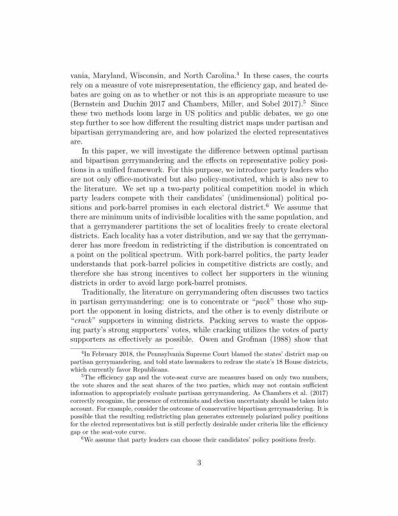
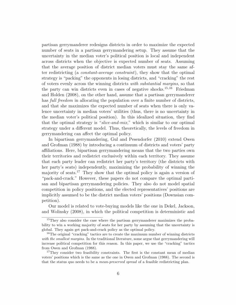
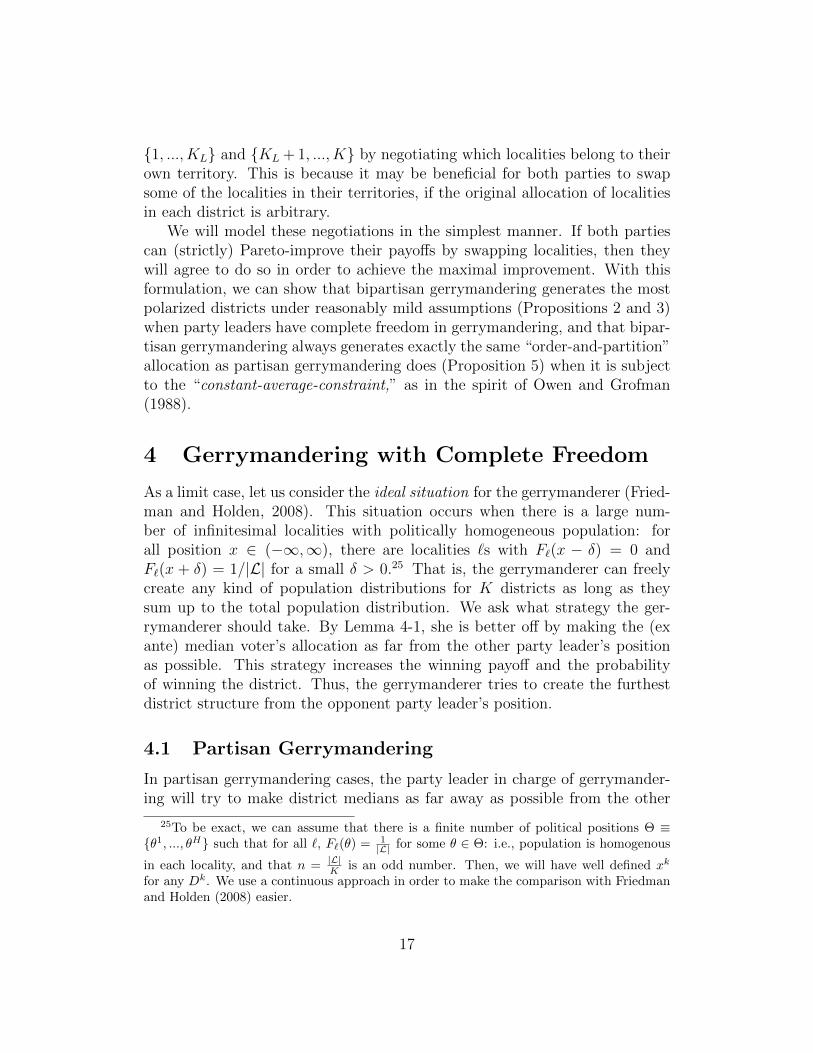
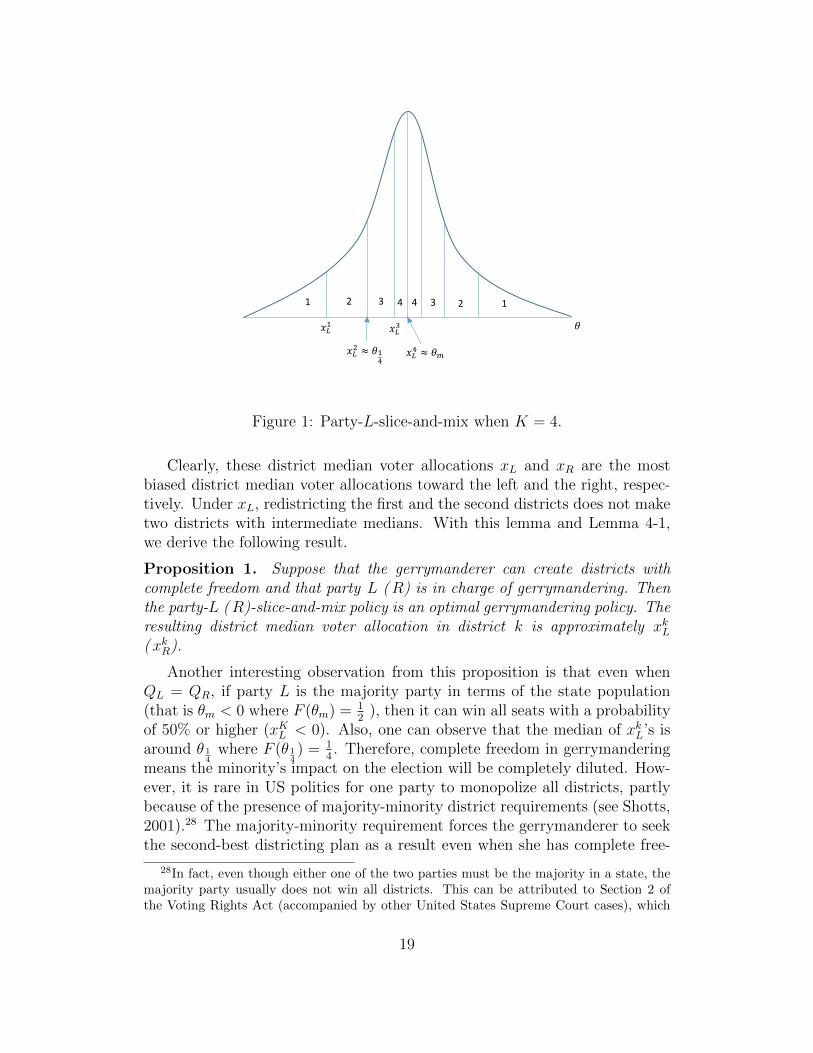
We call this redistricting plan a party-L-slice-and-mix policy, which is pro-posed in Friedman and Holden (2008). Under the slice-and-mix policy, theresulting district median voter allocation is xL ≡ (x1
L, ..., xKL ) with xkL is such
that F (xkL) = k2K
for each k = 1, ..., K. We will show that this is the optimalpolicy for the leader of party L. Figure 1 is an example of party-L-slice-and-mix strategy when K = 4. District k = 1, ..., 4 is composed of two slicesnumbered by k. District median voter allocation is xL ≡ (x1
L, ..., x4L).
The following result is straightforward: in order for xk to be the medianvoter in district k = 1, ..., K, xk must satisfy F (xk) ≥ k
2Kand 1−F (xk) ≥ k
2K.
(We define xR = (x1R, ..., x
KR ) in a perfectly symmetric way.)
Lemma 5. There is no (ex ante) median voter allocation x = (x1, ..., xK) withx1 ≤ x2 ≤ ... ≤ xK such that xk < xkL for any k = 1, ..., K. Symmetrically,there is no median voter allocation x = (x1, ..., xK) with x1 ≥ x2 ≥ ... ≥ xK
such that xk > xkR for any k = 1, ..., K.
26As long as there are positive winning probabilities in all districts (if y is large enough),this is true. If not, party L’s leader may need to create unwinnable districts, but she wouldbe indifferent as to how to draw lines for these districts. Even in this case, however, theslice-and-mix below is one of the optimal strategies.
27If we use the exactly finite setup described in footnote 25, then we can have a perfectlyconsistent model with a well-behaved optimal strategy with exact district median voters.We thank the associate editor for pointing this out. We decided to stick to a continuumapproximation, just to make the comparison with Friedman and Holden (2008) easier.
18
1 1 2 2 3 3 4
3
4
3
𝑥𝐿1
𝑥𝐿2 ≈ 𝜃1
4
𝑥𝐿3
𝑥𝐿4 ≈ 𝜃𝑚
𝜃
Figure 1: Party-L-slice-and-mix when K = 4.
Clearly, these district median voter allocations xL and xR are the mostbiased district median voter allocations toward the left and the right, respec-tively. Under xL, redistricting the first and the second districts does not maketwo districts with intermediate medians. With this lemma and Lemma 4-1,we derive the following result.
Proposition 1. Suppose that the gerrymanderer can create districts withcomplete freedom and that party L (R) is in charge of gerrymandering. Thenthe party-L (R)-slice-and-mix policy is an optimal gerrymandering policy. Theresulting district median voter allocation in district k is approximately xkL(xkR).
Another interesting observation from this proposition is that even whenQL = QR, if party L is the majority party in terms of the state population(that is θm < 0 where F (θm) = 1
2), then it can win all seats with a probability
of 50% or higher (xKL < 0). Also, one can observe that the median of xkL’s isaround θ 1
4where F (θ 1
4) = 1
4. Therefore, complete freedom in gerrymandering
means the minority’s impact on the election will be completely diluted. How-ever, it is rare in US politics for one party to monopolize all districts, partlybecause of the presence of majority-minority district requirements (see Shotts,2001).28 The majority-minority requirement forces the gerrymanderer to seekthe second-best districting plan as a result even when she has complete free-
28In fact, even though either one of the two parties must be the majority in a state, themajority party usually does not win all districts. This can be attributed to Section 2 ofthe Voting Rights Act (accompanied by other United States Supreme Court cases), which
19
dom. It is worthwhile to note that the slice-and-mix strategy is identical to theoptimal policy analyzed in Friedman and Holden (2008), although Friedmanand Holden do not include competition with political positions nor pork-barrelpolitics.
4.2 Bipartisan Gerrymandering
The preexisting territories of parties L and R are the districts they won inthe previous election, described by KL and KR = K −KL, respectively, andtheir territory-wise population distributions are described by FL(θ) and FR(θ),respectively, with (i) F (θ) = FL(θ)+FR(θ) for all θ, (ii) FL(∞) = KL× n
|L| , and
(iii) FR(∞) = KR × n|L| .
29 Through minor abuse of notation, let x0L =∞ and
θxkL be such that FL(xkL) = k2K
, and let zkL be such that FL(∞)−FL(zkL) = k2K
for k = 1, ..., KL by applying the same method for territories as in the previoussection. Similarly, let z0
R = −∞ and zkR be such that FR(zkR) = k−KL2K
, and let
xkR be such that FR(∞)− FR(xkR) = k−KL2K
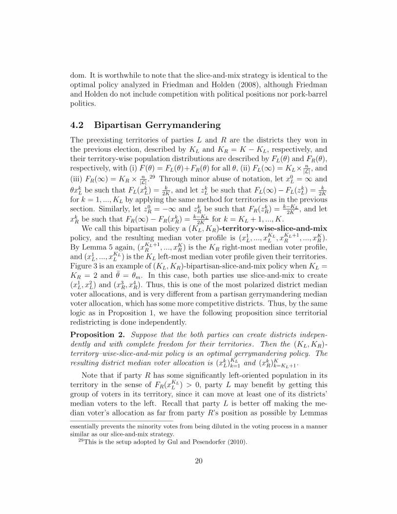
for k = KL + 1, ..., K.We call this bipartisan policy a (KL, KR)-territory-wise-slice-and-mix
policy, and the resulting median voter profile is (x1L, ..., x
KLL , xKL+1
R , ..., xKR ).By Lemma 5 again, (xKL+1
R , ..., xKR ) is the KR right-most median voter profile,and (x1
L, ..., xKLL ) is the KL left-most median voter profile given their territories.
Figure 3 is an example of (KL, KR)-bipartisan-slice-and-mix policy when KL =KR = 2 and θ = θm. In this case, both parties use slice-and-mix to create(x1
L, x2L) and (x3
R, x4R). Thus, this is one of the most polarized district median
voter allocations, and is very different from a partisan gerrymandering medianvoter allocation, which has some more competitive districts. Thus, by the samelogic as in Proposition 1, we have the following proposition since territorialredistricting is done independently.
Proposition 2. Suppose that the both parties can create districts indepen-dently and with complete freedom for their territories. Then the (KL, KR)-territory–wise-slice-and-mix policy is an optimal gerrymandering policy. Theresulting district median voter allocation is (xkL)KLk=1 and (xkR)Kk=KL+1.
Note that if party R has some significantly left-oriented population in itsterritory in the sense of FR(xKLL ) > 0, party L may benefit by getting thisgroup of voters in its territory, since it can move at least one of its districts’median voters to the left. Recall that party L is better off making the me-dian voter’s allocation as far from party R’s position as possible by Lemmas
essentially prevents the minority votes from being diluted in the voting process in a mannersimilar as our slice-and-mix strategy.
29This is the setup adopted by Gul and Pesendorfer (2010).
20

𝐹𝐿(𝜃) 𝐹𝑅(𝜃)
𝑥𝐿1 𝑥𝐿
2 𝑧𝐿2 𝑧𝐿
1
Figure 2: fL(θ) and fR(θ) are territory-wise locality distribution densities.Given these distributions, L applies slice-and-mix strategy, and x1
L and x2L are
the median voters in district 1 and 2. Notice that FR(x2L) (represented by the
shadowed area) allows L to create more extreme median voters in districts 1and 2. The same incentive exists for R in this example. So, swapping localitiesis Pareto-improving.
3-1 and 4-1. See Figure 2 for an example. The same is true for party R ifFL(∞) − FL(xKL+1
R ) > 0.30 If uncertainty y is small, then there is no un-certainty in district elections, and bipartisan gerrymandering benefits fromswapping these localities. The following proposition illustrates this mutuallybeneficial negotiation between the two parties since party leaders do not careabout the opponent party’s policy positions in losing districts.
Proposition 3. Suppose that the resulting district median voter allocationis approximately (xkL)KLk=1 and (xkR)Kk=KL+1 under the (KL, KR)-territory–wise-
slice-and-mix policy. Suppose that (i) FR(xKLL ) > 0 and FL(∞)−FL(xKL+1R ) >
0 hold, and (ii) y satisfies y ≤ min{∣∣xKLL ∣∣ , ∣∣xKL+1
R
∣∣}. Then, the two partiesbenefit from swapping these localities in a bipartisan negotiation between them.
Condition (ii) says that party L wins in districts k = 1, ..., KL, and partyR wins in districts k = KL+1, ..., K with certainty. Then, both parties arebetter off having more extreme polarizations in their winning districts, aslong as parties do not care about policies in losing districts. If this swappingincentive exists, both parties would continue to do so until FR(xKLL ) = 0 and
30Note that the median voters in created districts are determined only by FL in interval(−∞, xKL
L ) and FR in interval (xKL+1R ,∞). The rest of the FL and FR distributions do not
make any difference under slice-and-mix.
21
1 3 2 4 2 4 3
3
1
3
𝑥𝐿1 𝑥𝐿
2
𝜃
𝑥𝑅1 𝑥𝑅
2
��
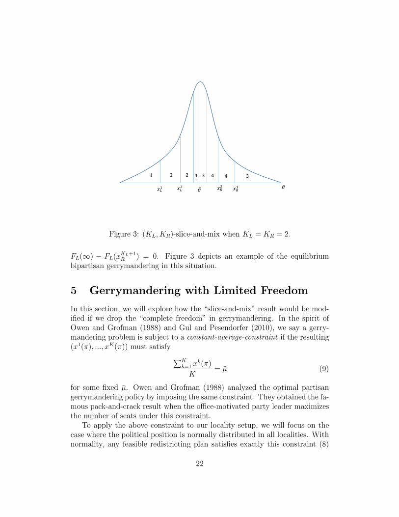
Figure 3: (KL, KR)-slice-and-mix when KL = KR = 2.
FL(∞) − FL(xKL+1R ) = 0. Figure 3 depicts an example of the equilibrium
bipartisan gerrymandering in this situation.
5 Gerrymandering with Limited Freedom
In this section, we will explore how the “slice-and-mix” result would be mod-ified if we drop the “complete freedom” in gerrymandering. In the spirit ofOwen and Grofman (1988) and Gul and Pesendorfer (2010), we say a gerry-mandering problem is subject to a constant-average-constraint if the resulting(x1(π), ..., xK(π)) must satisfy ∑K
k=1 xk(π)
K= µ (9)
for some fixed µ. Owen and Grofman (1988) analyzed the optimal partisangerrymandering policy by imposing the same constraint. They obtained the fa-mous pack-and-crack result when the office-motivated party leader maximizesthe number of seats under this constraint.
To apply the above constraint to our locality setup, we will focus on thecase where the political position is normally distributed in all localities. Withnormality, any feasible redistricting plan satisfies exactly this constraint (8)
22

(the proof is obvious when we note that the median is equivalent to the meanunder normality).
Lemma 6. Suppose that the voter distribution in each locality is normallydistributed, i.e., F` ∼ N(µ`, σ`) for each ` ∈ L. Then, the median of districtk is
xk(π) =1
n
∑`∈Dk(π)
µ`.
Moreover, for all π ∈ Π,∑Kk=1 x
k(π)
K= θm = µ.
With this lemma, we can identify the optimal gerrymandering strategy fora special case. Starting from a district partition π with h, k ∈ {1, ..., K} andxk(π) ≤ xh(π), consider swapping a pair of localities ` ∈ Dk(π) and ˜∈ Dh(π)with µ˜< xk(π) ≤ xh(π) < µ`. Let the outcome of this redistricting be π′: i.e.,
Dk(π′) = Dk(π) ∪ {˜}\{`}, Dh(π′) = Dh(π) ∪ {`}\{˜}, and Dk(π) = Dk(π)for all k 6= k, h. From the above formula, it is clear that xk(π′) < xk(π) ≤xh(π) < xh(π′).
Which plan should the party leader (say, party L’s leader) choose betweenπ and π′? The answer depends on the shape of EVi. It is obvious that ifEVi is a convex function in the ex ante median voter’s position xk, the partyleader would prefer π′ to π as long as k ∈ KL. As we have seen in Lemma4-3, if the third derivatives of cost functions are positive, party leaders haveconvex expected payoff functions, and they prefer more heterogenous districtsin median voters’ positions to homogenous districts.31
In this case, it is easy to characterize the optimal partisan gerrymanderingpolicy with limited freedom. Let a district partition π = {D1(π), ..., DK(π)}such that for all k = 1, ..., K ′ and all h = 2, ..., K with k < h, all ` ∈ Dk(π) and˜∈ Dh(π), µ` ≤ µ˜ holds, where K ′ is such that for all districts k > K ′, thereis absolutely no chance for party L to win: xK
′(π)− y < 0 but xk(π)− y > 0 for
all k > K ′. We call this allocation π an order-and-partition gerrymanderingpolicy. This policy packs the most opposing localities in unwinnable districts,and partitions the rest of the localities into consecutive locality districts. ByLemma 4-2, we have the following result.
Proposition 4. Suppose that the voter distribution is normal in each localityand QL = QR. In addition, suppose that C ′′′(·) ≥ 0 and c′′′(·) ≥ 0 hold. Then,the optimal partisan gerrymandering policy is order-and-partition (xk)K
′
k=1 withpacking in the unwinnable districts. In particular, (xk)Kk=1 is one of the optimal
31The relevant case is h ∈ KL. If h /∈ KL, it is obvious that party L prefers π′ to π.
23

partisan gerrymandering policies. If K ′ = K, the unique optimal policy isorder-and-partition (xk)Kk=1.
Thus, cracking is not necessarily a good strategy here, unlike in Owen andGrofman (1988). The difference between the current paper and theirs is thatour party leaders are also policy-motivated.32 What about the case whereC ′′′(·) ≥ 0 and c′′′(·) ≥ 0 do not hold? Actually, we can show that V k
i isconcave if C ′′′(·) ≤ 0 and c′′′(·) ≤ 0, so it appears that pack-and-crack is theway to go. Indeed, it is true for the deterministic case (y = 0) or for caseswhere y is small enough. However, even if the third derivatives are negative,EV k
L can be convex, as is seen in the following example (see also Appendix B).
Example 1. We introduce a convenient special ideology cost function suchthat both voters’ and party leaders’ cost functions have common constantelasticity. Let C(d) = aCdγ and c(d) = acdγ, where γ > 1, aC > 0, and ac > 0are parameters. In this case, both party leaders and voters have the sameelasticity that is constant γ. This conveniently yields the following formula.
Denote A = A(aC , ac) = aC(
α1+α
)γ+ ac
(1
1+α
)γ> 0 where α =
(aC
ac
) 1γ−1
. We
can choose aC and ac to set A = 1 for each γ: then we have C(d) = Adγ = dγ.In this case, V k
L is concave (convex) in xk if γ ≤ 2 (γ ≥ 2). Suppose thatθL = −1, θR = 1 (thus L wins if and only if xk < 0), and g(y) = 1
2yif and
only if y ∈ [−y, y] (uniform distribution). Also, suppose that all possible xk
are in [−1, 1] and(QA
) 1γ ≥ 2 + y holds to satisfy Assumption 2. If y > 1, there
is always a chance to win the election: we have xk − y < 0 and xk + y > 0. Inthis case,
EV k′′L =
γ
2y[(1− xk + y)γ−1 − (−1− xk + y)γ−1] > 0.
For all γ > 1, (1−xk+y)γ−1−(−1−xk+y)γ−1 > 0 holds. Thus, the expectedutility is convex in xk, even if γ < 2 or C ′′′(d) < 0. This example showsthat even without positive third derivatives, the order-and-partition strategyis optimal for the constrained case with the constant average constraint.�
We now set our sights on bipartisan gerrymandering. In Section 4.2, weargue that when y is not large enough to change the district winners, parties
32Without the policy motivation, the payoff function is only related to winning prob-ability, and pack-and-crack is optimal under a mild assumption on g. See also Gul andPesendorfer (2010).
24

have incentives to swap localities as long as the swap can increase the abilityof both parties to create extreme districts in the redistricting stage. A similaridea applies to the constrained gerrymandering case. Suppose that EV k isconvex (it is assured if the third derivatives of cost functions are positive).Suppose also that there exist ` and ˜ with ` ∈ Dk, ˜∈ Dh, and µ` > µ`′ , andthat districts k and h belong to parties L and R, respectively. By swapping `and ˜, parties L and R can make xk and xh decrease and increase by the samemagnitude, respectively. This is strictly Pareto-improving for both parties.Therefore, the two parties should agree to form consecutive territories in stage0.
Then, in stage 1, both party leaders adopt order-and-partition in their ownconsecutive territory; it does not matter whether redistricting is conducted bya partisan or bipartisan committee. This observation shows that for the ger-rymandering problem with limited freedom, bipartisan gerrymandering doesnot create a more polarized allocation than partisan gerrymandering, and in-cumbents’ re-election rates would be the same.
Proposition 5. Suppose that the voter distribution is normal in each localityand QL = QR. In addition, suppose that C ′′′(·) ≥ 0 and c′′′(·) ≥ 0 hold. Then,the optimal bipartisan gerrymandering policy is order-and-partition (xk)Kk=1,which is identical to the partisan policy.
The constant average constraint forbids a gerrymanderer from diluting sup-porters of the other party by mixing in his own supporters. Notice that whilegerrymanderer L can pull the median of district medians to θ 1
4in the complete
freedom case, the median of medians has to remain as θm, the population me-dian, when the constant average constraint applies. Propositions 4 and 5 echoFriedman and Holden (2009), in which the insignificant difference between par-tisan and bipartisan gerrymandering is a possible consequence of the VotingRights Act of 1982, which significantly limits the gerrymanderer’s ability todilute votes.
6 Conclusion
In this paper, we propose a gerrymandering model in which candidates com-pete with their policy positions and pork-barrel politics, and analyze the rela-tionship between gerrymandering and policy polarizations. In the context ofgerrymandering, this is the first paper to introduce policy motivations as wellas office motivations. The model’s tractability allows us to compare the perfor-mance of partisan and bipartisan gerrymandering under different constraints.
25

We show that gerrymandering may play some role in polarizing candidates’policy positions.
In the main text, we assumed that party leaders do not care about policieschosen by the opponent in their losing districts. Although this assumptionmay make sense in the context of gerrymandering, it would be interesting tosee how our results are affected by weakening this assumption, since manymodels in electoral competition assume that losing candidates also care aboutpolicy realizations, as in a seminal paper by Wittman (1983). In AppendixC, we conduct a robustness check for analyzing the case of σ > 0 in (4).Although election equilibria are affected by this modification, the modificationsare just parallel reductions of equilibrium winning payoffs. This is becauselosing payoffs are changed from zero to the disutility levels from the opponentparties’ policy choices. When σ is large, both Lemma 4.1 and Lemmas 4.2and 4.3 can be violated, which can cause problems for our results. However,if σ is not large, then all the results including Example 1 hold. In numericalcalculations, it seems safe to say that our results hold for significantly widerange of σ (see Appendix C).
There are some potentially interesting yet difficult avenues for further re-search. First, one may want to introduce uncertainty in election results (e.g.,uncertainty in the median voter’s position after policy proposal) into ourmodel. If uncertainty is infinitesimal (e.g., if the gerrymander can only observethat the median voter’s position belongs to the interval [xk − ε, xk + ε] for εbeing a (small) preference perturbation) and if the gerrymanderer has com-plete freedom in redistricting, the slice-and-mix strategy may still be optimal,a la Friedman and Holden (2008). However, with significant uncertainty inmedian voters’ positions, as in Gul and Pesendorfer (2010), we cannot predictwhat will happen.
Second, in this paper we concentrated on one type of pork-barrel politics:candidates’ “promise” transfers contingent on their winning of the districts.These kinds of promises are different from campaign expenditures. In the lat-ter case, even if a candidate loses in a district, the spent campaign expenditurewill not come back (an all-pay auction). In some circumstances, such a modelmay be more realistic if there is uncertainty in the election results. How-ever, introducing uncertainty in election results is not trivial, as we mentionedbefore. These issues are left for future research.
26

Appendix A: Proofs
Proof of Lemma 1. First, by Assumption 2, the non-negativity constraintof tkR is not needed. Second, in any equilibrium, the median voter is indifferentto L and R’s proposals and votes for the candidate who yields higher payoffs.Suppose not, without loss of generality, let QL − tkL − C(|βkL − θL|) > QR −tkR − C(|βkR − θR|) = 0 and the median voter votes for L with probability lessthan 1. Then, L can win for sure by promise tkL + ε. Then, voting for L withprobability less than 1 cannot be an equilibrium.
Then, there are three cases: if R loses with QR − tk∗R − C(
∣∣θR − βk∗R ∣∣) > 0and its offer gives the median voter utility equal to U in equilibrium, it mustbe that L wins with positive indirect utility and also provides the median voterwith the utility level U . However, this means that R can win the election byproviding, say, ε more pork-barrel promises. This contradicts the equilibriumcondition. The second case is that Q− tk∗R − C(
∣∣θR − βk∗R ∣∣) = 0 but Uxk(R) isnot maximized. In this case, there must exist some points (t′, β′) that satisfyQ − t′ − C(|θR − β′|) = 0, but the pair provides the median voter strictlyhigher utility. In this case, any point on the segment connecting (t′, β′) and(tk∗R , β
k∗R ) is strictly better off for both R and the median voter xk by the strict
convexity of the preferences. Again, this contradicts the equilibrium condition.The third case, Q− tk∗R −C(
∣∣θR − βk∗R ∣∣) < 0, cannot happen, since the strategythat generates a negative payoff is a weakly dominated strategy for R’s leader.�
Proof of Lemma 2. We only need to prove Lemma 2-3. We consider two
cases: (Case-1) xk > θi, and (Case-2) xk < θi.(Case-1): In this case, βi = β(xk, θi) is determined implicitly by the first-
order conditionC ′(βi − θi) = c′(xk − βi)
Totally differentiating with respect to xk and βi, we obtain
(C ′′ + c′′)dβi = c′′dxk
(Case-2): In this case, βi = β(xk, θi) is determined implicitly by the first-order condition
C ′(θi − βi) = c′(βi − xk)
Totally differentiating with respect to xk and βi, we obtain
(C ′′ + c′′)dβi = c′′dxk
27
Thus, we get the same condition either way. We have completed the proof.�
Proof of Lemma 3. We will focus on the case of i = L. When i = R, wecan apply the same procedure. We will first show the following claim.
Claim. C ′i = c′i when θi < xk, C ′i = −c′i when θi > xk and C ′′i =c′′i C
′′i
c′′i +C′′i, where
Ci = C(∣∣xk − θi∣∣), ci = c
(∣∣∣xk − βi (xk, θi)∣∣∣), and Ci = C(∣∣∣βi (xk, θi)− θi∣∣∣).
Proof of Claim. So, there are two cases: (Case-a) θi < xk, and (Case-b)θi > xk.(Case-a): Taking the first derivative, we have
C ′(xk − θi) = C ′(βi − θi)∂βi∂xk
+ c′(xk − βi)(1−∂βi∂xk
) = c′(xk − βi),
Here, we used the first-order condition C ′ = c′, which must hold at the opti-mum. Taking the second-order derivative, we have
C ′′(xk − θi) = c′′(xk − βi)(1−∂βi∂xk
)
= c′′(xk − βi)
(1− c′′(xk − βi)
c′′(xk − βi) + C ′′(βi − θi)
)
=c′′(xk − βi)C ′′(βi − θi)c′′(xk − βi) + C ′′(βi − θi)
(Case-b): Taking the first-order derivative, we have
C ′(θi − xk) = −C ′(θi − βi)∂βi∂xk
+ c′(βi − xk)(∂βi∂xk− 1) = −c′(βi − xk),
Taking the second-order derivative, we have
C ′′(θi − xk) = −c′′(βi − xk)(∂βi∂xk− 1)
= c′′(βi − xk)
(1− c′′(xk − βi)
c′′(xk − βi) + C ′′(θi − βi)
)
=c′′(βi − xk)C ′′(θi − βi)c′′(βi − xk) + C ′′(θi − βi)
We have completed the proof of the Claim.�
28

We start with Lemma 3-1. First, we consider (Case-1): xk ∈ (θL, θR),then V k
L = (QL −QR)−(C(xk + y − θL)− C(θR − xk − y)
). Thus, we have
dV kL
dxk= −
(C ′(xk − θL) + C ′(θR − xk)
)< 0.
This implies that V kL is decreasing in xk. In the case of V k
R ,dV kRdxk
> 0 and V kR is
increasing in xk.There are two more cases: (Case-2) xk < θL, and (Case-3) xk > θR.
(Case-2):dV kLdxk
= C ′(θL − xk)− C ′(θR − xk) < 0, since C ′′(d) > 0. Thus, V kL is
decreasing in xk.
(Case-3):dV kLdxk
= −C ′(xk − θL) + C ′(xk − θR) < 0, since C ′′(d) > 0. Thus, V kL
is decreasing in xk.For the convexity, again we have three cases: (Case-1) xk ∈ (θL, θR),
(Case-2) xk < θL, and (Case-3) xk > θR. In each case, we have the samesecond-order derivatives:(Case-1):
d2V kLd(xk)2
= −C ′′(xk − θL) + C ′′(θR − xk).
(Case-2):dV kLdxk
= C ′(θL− xk)−C ′(θR− xk) andd2V kLd(xk)2
= −C ′′(θL− xk)+C ′′(θR−xk).
(Case-3):dV kLdxk
= −C ′(xk − θL) + C ′(xk − θR) andd2V kLd(xk)2
= −C ′′(xk − θL) +
C ′′(xk − θR).
Therefore, in all cases,d2V kLd(xk)2
= −C ′′L + C ′′R, so we have:
d2V kL
d(xk)2= −C ′′L + C ′′R
= − c′′LC′′L
c′′L + C ′′L+
c′′RC′′R
c′′R + C ′′R
=−c′′LC ′′L (c′′R + C ′′R) + c′′RC
′′R (c′′L + C ′′L)
(c′′L + C ′′L) (c′′R + C ′′R)
=C ′′LC
′′R (c′′R − c′′L) + c′′Lc
′′R (C ′′R − C ′′L)
(c′′L + C ′′L) (c′′R + C ′′R)
Thus, if c′′R ≥ c′′L and C ′′R ≥ C ′′L thend2V kLd(xk)2
≥ 0. Since QL = QR, if L wins,
then xk − θL < θR − xk. Thus, if c′′′ > 0 and C ′′′ > 0 then we have c′′R ≥ c′′Land C ′′R ≥ C ′′L.�
Proof of Lemma 4. We will focus on the case of i = L. When i = R, wecan apply the same procedure. Let’s start with Lemma 4-1. Consider the case
29
where xk ± y ∈ (θL, θR). There are two subcases: (Case 1) is the case whereL wins with certainty (V k
L (xk + y, θL, θR) ≥ 0), and (Case 2) is the one whereL may lose depending on the realization of y (V k
L (xk + y, θL, θR) < 0).
(Case 1): In this case, EV kL =
∫ y−y V
kL (xk + y, θL, θR)g(y)dy. Thus,
dEV kL
dxk=
∫ y
−yV k′L (xk + y, θL, θR)g(y)dy < 0
where V k′L =
dV kLdxk
=dV kLdxk
.
(Case 2): In this case, EV kL =
∫ x−xk−y V k
L (xk+y, θL, θR)g(y)dy, where V kL (x, θL, θR) =
0. That is, if xk + y > x, then party L loses. (Note that x is solely determinedby the value of QL −QR: dx
d(QL−QR)> 0. If QL = QR, then x = 0 holds, since
θL = −θR.) Differentiating this with respect to xk, we have
dEV kL
dxk= V k
L (0, θL, θR)g(−xk) +
∫ x−xk
−yV k′L (xk + y, θL, θR)g(y)dy
=
∫ x−xk
−yV k′L (xk + y, θL, θR)g(y)dy < 0
Thus, we have completed the proof of Lemma 4-1.For Lemma 4-2, we classify four cases:
(Case a: xk − y ≥ θL and xk + y ≤ x): In this case, EV kL =
∫ y−y V
kL (xk +
y, θL, θR)g(y)dy. Thus,
d2EV kL
d(xk)2=
∫ y
−yV k′′L (xk + y, θL, θR)g(y)dy
(Case b: xk − y ≥ θL and xk + y > x): In this case, EV kL =
∫ −xk−y V k
L (xk +
y, θL, θR)g(y)dy. That is, if xk +y > x = 0, then party L loses. Differentiatingthis with respect to xk, we have
dEV kL
dxk= −V k
L (0, θL, θR) +
∫ −xk−y
V k′L (xk + y, θL, θR)g(y)dy
=
∫ −xk−y
V k′L (xk + y, θL, θR)g(y)dy
30

Thus, the second-order derivative is
d2EV kL
d(xk)2= −V k′
L (0, θL, θR) +
∫ −xk−y
V k′′L (xk + y, θL, θR)g(y)dy
From Lemma 3-2, we know V k′L (0, θL, θR) < 0 and V k′′
L (xk + y, θL, θR) > 0.Thus, EV k
L is convex.
(Case c: xk − y < θL and xk + y ≤ x): In this case, EV kL =
∫ θL−xk−y V k
L (xk +
y, θL, θR)g(y)dy +∫ yθL−xk
V kL (xk + y, θL, θR)g(y)dy. Differentiating this with
respect to xk, we obtain
dEV kL
dxk=
∫ θL−xk
−yV k′L (xk + y, θL, θR)g(y)dy +
∫ y
θL−xkV k′L (xk + y, θL, θR)g(y)dy
The second-order derivative is
d2EV kL
d(xk)2=
∫ θL−xk
−yV k′′L (xk + y, θL, θR)g(y)dy+
∫ y
θL−xkV k′′L (xk + y, θL, θR)g(y)dy
From Lemma 3-2, we know V k′L (0, θL, θR) < 0 and V k′′
L (xk + y, θL, θR) > 0.Thus, EV k
L is convex.
(Case d: xk − y < θL and xk + y > x): In this case, EV kL =
∫ θL−xk−y V k
L (xk +
y, θL, θR)g(y)dy +∫ −xkθL−xk
V kL (xk + y, θL, θR)g(y)dy. Differentiating this with
respect to xk, we obtain
dEV kL
dxk=
∫ θL−xk
−yV k′L (xk + y, θL, θR)g(y)dy +
∫ −xkθL−xk
V k′L (xk + y, θL, θR)g(y)dy
− V kL (0, θL, θR)g(−xk)
=
∫ θL−xk
−yV k′L (xk + y, θL, θR)g(y)dy +
∫ −xkθL−xk
V k′L (xk + y, θL, θR)g(y)dy
The second-order derivative is
d2EV kL
d(xk)2=
∫ θL−xk
−yV k′′L (xk + y, θL, θR)g(y)dy +
∫ −xkθL−xk
V k′′L (xk + y, θL, θR)g(y)dy
−V k′L (0, θL, θR)g(−xk)
From Lemma 3-2, we know V k′L (0, θL, θR) < 0 and V k′′
L (xk+y, θL, θR) > 0 whenc′′(d) > 0 and C ′′(d) > 0. Thus, EV k
L is convex. We have completed the proofof Lemma 4-2.
31

For Lemma 4-3, first observe that,
EVi (π) ≡∫ y
−y
K∑k=1
max{V ki (xk(π) + y, θi, θj), 0
}g(y)dy
For any k 6= k′, ∂2EVi∂xk∂xk′
= 0. The Hessian matrix of EVL has zeros on non-diagonal parts and negative terms on the diagonal due to Lemma 4-2. There-fore, the Hessian matrix is negative semidefinite and EV are convex functionin (xk)Kk=1. �
Proof of Lemma 5. Note that F (xkL) = k2K
. Thus, to achieve xkL as themedian voter of the kth district, we need to use all voters to the left of xkL. Thisis true for all k = 1, ..., K. Thus, xL is the leftmost median voter allocationin lexicographic order. We can prove the statement for xR by a symmetricargument.�
Proof of Proposition 4. Suppose that a district structure π is not “order-and-partition.” We will show that π is not an optimal partisan gerrymanderingpolicy when the third derivatives of cost functions are positive. Since π is notorder-and-partition, there exist districts k and h such that there exist ` ∈ Dk
and ˜ ∈ Dh with µ` > µ˜, in which one of the following holds: (Case-I)k, h ≤ K ′ and xk(π) ≤ xh(π), or (Case-II) k ≤ K ′ and h > K ′. Let π′
be a district structure that is generated by swapping localities ` and ˜ of π.Let’s start with (Case-I). In this case, xk(π′) < xk(π) ≤ xh(π) < xh(π′) holds.Thus, by Lemma 4-3, EVL(π) < EVL(π′). (Case-II) is simpler. In this case, itis obvious that xk(π′) < xk(π) holds. Thus, by Lemma 4-1, EVL(π) < EVL(π′)holds. We conclude that the optimal partisan gerrymandering policy is order-and-partition.�
Appendix B: Constant Elasticity Example
In this appendix, we elaborate on the calculation involved in Example 1. LetC(d) = aCdγ and c(d) = acdγ, where γ > 1, aC > 0, and ac > 0 are parameters.In this case both party leaders and voters have the same constant elasticityγ. Thus, we have the following convenient formula. Denote A = A(aC , ac) =
aC(
α1+α
)γ+ ac
(1
1+α
)γ> 0 where α =
(aC
ac
) 1γ−1
. Suppose that(QA
) 1γ ≥ 2 + y
holds to satisfy Assumption 2. Normalizing A = 1, we have C(d) = Adγ = dγ.In this case, V k
L is concave (convex) in xk if γ ≤ 2 (γ ≥ 2).
32
EV kL =
∫ −xkθL−xk
(C(θR − xk − y)− C(xk + y − θL)
)g(y)dy
+
∫ θL−xk
−y
(C(θR − xk − y)− C(θL − xk − y)
)g(y)dy
dEV kL
dxk=
∫ −xkθL−xk
(−C ′(θR − xk − y)− C ′(xk + y − θL)
)g(y)dy
+
∫ θL−xk
−y
(−C ′(θR − xk − y) + C ′(θL − xk − y)
)g(y)dy
d2EV kL
d(xk)2=
∫ −xkθL−xk
(C ′′(θR − xk − y)− C ′′(xk + y − θL)
)g(y)dy
+
∫ θL−xk
−y
(C ′′(θR − xk − y)− C ′′(θL − xk − y)
)g(y)dy
+ (C ′(θR) + C ′(−θL))g(−xk)Suppose that C(d) = dγ (γ > 1), θL = −1, θR = 1 (thus x = 0), and g(y) = 1
2y
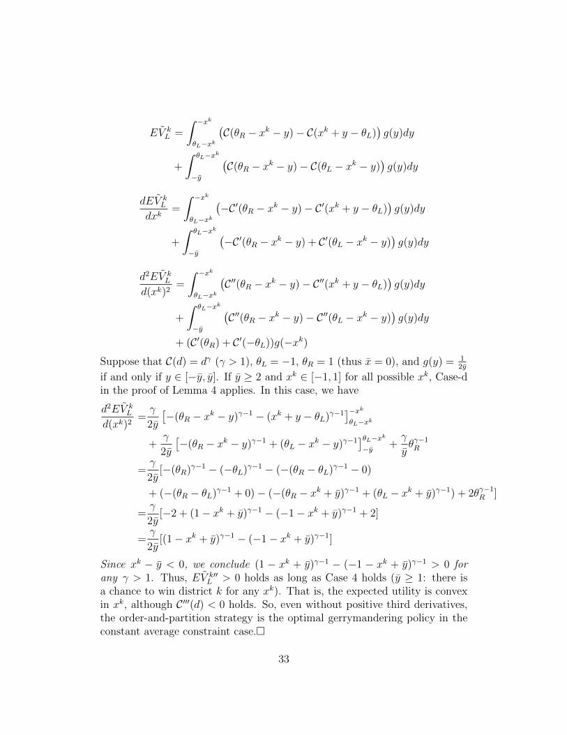
if and only if y ∈ [−y, y]. If y ≥ 2 and xk ∈ [−1, 1] for all possible xk, Case-din the proof of Lemma 4 applies. In this case, we have
d2EV kL
d(xk)2=γ
2y
[−(θR − xk − y)γ−1 − (xk + y − θL)γ−1
]−xkθL−xk
+γ
2y
[−(θR − xk − y)γ−1 + (θL − xk − y)γ−1
]θL−xk−y +
γ
yθγ−1R
=γ
2y[−(θR)γ−1 − (−θL)γ−1 − (−(θR − θL)γ−1 − 0)
+ (−(θR − θL)γ−1 + 0)− (−(θR − xk + y)γ−1 + (θL − xk + y)γ−1) + 2θγ−1R ]
=γ
2y[−2 + (1− xk + y)γ−1 − (−1− xk + y)γ−1 + 2]
=γ
2y[(1− xk + y)γ−1 − (−1− xk + y)γ−1]
Since xk − y < 0, we conclude (1 − xk + y)γ−1 − (−1 − xk + y)γ−1 > 0 forany γ > 1. Thus, EV k′′
L > 0 holds as long as Case 4 holds (y ≥ 1: there isa chance to win district k for any xk). That is, the expected utility is convexin xk, although C ′′′(d) < 0 holds. So, even without positive third derivatives,the order-and-partition strategy is the optimal gerrymandering policy in theconstant average constraint case.�
33

Appendix C
In the benchmark model, we assume that the losing payoff of a candidate is 0.In this section, we extend our model to a general setup a la Wittman (1983).Formally, by losing in district k, party j’s leader gets utility
V kj = −σC(|βki − θj|)
where σ ∈ [0, 1] naturally (candidate cares about her own policy more thanher opponent’s policy). Supposing that the winning party is L, the winner’smaximization problem (5) is not changed. Therefore, the optimal strategycombination is still βL(xk, θL) and tk
∗L (Uk
R) = UkR + c(|xk − βL(xk, θL)|). From
Lemma 1, the losing R chooses an equilibrium strategy combination as if hetried to maximize the median voter’s payoff given its utility of no less than−σC(|βkL − θR|). Formally, R solves the following problem
maxβkR,t
kR
Uxk(R) = tkR − c(|xk − βkR|)
subject to tkR ≥ 0 and QR − tkR − C(∣∣θR − βkR∣∣) ≥ −σC(|βkL − θR|).
Notice that, since the losing payoff is negative, the losing party promises moreaggressively to the median voter to maximize her chance of winning in a weaklyundominated strategy. When the second constraint is binding, the problembecomes
maxβkR
QR − C(∣∣θR − βkR∣∣)− c(|xk − βkR|) + σC(|βkL − θR|).
Thus, R again chooses βkR, which is a function of xk and θR minimizingC(∣∣θR − βkR∣∣) + c(|xk − βkR|). On the other hand, since the winning candidate
L tries to maximize her payoff QL−C(∣∣θL − βkL∣∣)− tkL = QL−C(
∣∣θL − βkL∣∣)−Uxk(R)− c(|xk − βkL|) by providing the median voter exactly the same utilityUxk(R) that candidate R assures, the equilibrium strategies are
βk∗
L = βL(xk, θL)
tk∗
L = QL −QR − C(∣∣∣θL − βL∣∣∣)− c(|xk − βL|) + C(|θR − βR|) + c(|xk − βR|)
− σC(|βL − θR|),
and
βk∗
R = βR(xk, θR) and tk∗
R = QR − C(|θR − βR|) + σC(|βL − θR|)
34

where βL(xk, θL) = arg minβC(|θL − β|) + c(|xk − β|). Since this is a simulta-
neous move game, candidate L does not take the externality to candidate Rinto account when she chooses β. Focusing on the case where QL = QR and|θL| = θR, candidate L’s winning payoff is
CR − CL − σC(|βL − θR|)
and L wins if and only if∣∣θL − xk∣∣ < ∣∣θR − xk∣∣. Therefore,
V kL =
{CR − CL − σC(|βL − θR|) if
∣∣θL − xk∣∣ < ∣∣θR − xk∣∣−σC(|βR − θL|) if
∣∣θL − xk∣∣ > ∣∣θR − xk∣∣We argue that Lemma 4 continues to hold if σ is small enough. We focus
on case (d) in the proof of Lemma 4, i.e., xk − y < θL and xk + y > 0. Forother cases, the proofs are similar. First,
EV kL =
∫ −xk−y
[CR − CL] g(y)dy − σ∫ −xk−y
C(|βL − θR|)g(y)dy
− σ∫ y
−xkC(|βR − θL|)g(y)dy
Therefore,
dEVLdxk
=− [−C(θR)− C(−θL)] g(−xk) +
∫ −xk−y
[−c′R(βR − (xk + y))− c′L((xk + y)− βL)
]g(y)dy
+ σC(θR − βL(0, θL))g(−xk) + σ
∫ −xk−y
C ′(θR − βL)∂βL∂xk
g(y)dy
− σC(βR(0, θR)− θL)g(−xk)− σ∫ y
−xkC ′(βR − θL)
∂βR∂xk
g(y)dy
=
∫ −xk−y
[−c′R(βR − (xk + y))− c′L((xk + y)− βL)
]g(y)dy
+ σ
[∫ −xk−y
C ′(θR − βL)∂βL∂xk
g(y)dy −∫ y
−xkC ′(βR − θL)
∂βR∂xk
g(y)dy
]
This may fail to be negative for xk around zero when σ is large, especially when−xk and y are close (the second term in the last bracket is small); i.e., L winsdistrict k with high probability. When σ is large, the negative first line can bedominated by the first term of the second line, which is the payoff suppression
35

effect caused by the loser’s payoff in electoral competition. Therefore, Lemma4.1 may fail to hold locally for xk around −y when σ is large enough (thesecond line has higher weight, and payoff suppression effect is large).
For the second derivative, we have
d2EV kL
d(xk)2=[c′(βR(0, θR)) + c′(−βL(0, θL))
]g(−xkL)
−∫ −xk−y
∂
∂xk
(c′R(βR − (xk + y)) + c′L((xk + y)− βL)
)g(y)dy
− σC ′(θR − βL(0, θL))∂βL∂xk
(0, θL)g(−xk)
− σ∫ xk
−y
C ′′(θR − βL)
(∂βL∂xk
)2
− C ′(θR − βL)∂2βL∂(xk)2
g(y)dy
− σC ′(βR(0, θR)− θL)∂βR∂xk
(0, θR)g(−xk)
− σ∫ y
−xk
C ′′(βR − θL)
(∂βR∂xk
)2
+ C ′(βR − θL)∂2βR∂(xk)2
g(y)dy
The first two terms are the same as the case where σ = 0 and are (strictly)positive. However, the signs of the third and fifth terms are negative and the
signs of all other terms are undetermined (the signs of ∂2βL∂(xk)2
and ∂2βR∂(xk)2
are
unknown), and it is impossible to determine the sign of the second derivativewhen σ is large. However, as long as σ is not large, Lemma 4.2 and 4.3 prevail.
Example 1 (continuation). In this case, we can write βL(xk, θL) = α1+α
xk +1
1+αθL and βR(xk, θR) = α
1+αxk + 1
1+αθR. Thus, we have
∂2βL∂(xk)2
=∂2βR∂(xk)2
= 0
and
d2EV kL
d(xk)2=
γ
2y
[(1− xk + y)γ−1 − (−1− xk + y)γ−1
]− σ γ
2y
α
1 + α
[(1− α
1 + α(xk − y) +
1
1 + α
)γ−1
+
(α
1 + α(xk + y) +
1
1 + α+ 1
)γ−1]
36

From Example 1, the first term is positive. However, all other terms arenegative ones multiplied by σ ∈ [0, 1]. Thus, the expected utility is convexin xk, when σ ≥ 0 is small enough. This is especially true, if we adopt the
wildly-used quadratic cost functions; i.e. γ = 2,d2EV kLd(xk)2
is linear, and the aboveequation is simplified:
d2EV kL
d(xk)2=γ
y
[1− σα
1 + α
{1 +
1
1 + α+
α
1 + αy
}]Therefore, readers can easily see the parameter space where our results hold.For example, when y = 1.5, α = 1, −y < xk < y, and σ < 2
3, EV k
L is convex.This example shows that even if candidates’ losing payoffs are negative, theorder-and-partition strategy can be optimal for the constrained case with theconstant average constraint.�
References
[1] Bernstein, M., and M. Duchin (2017): “A Formula Goes to Court: Par-tisan Gerrymandering and the Efficiency Gap,” Notice of the AmericanMathematical Society 64(9), pp. 1020-1024.
[2] Besley, T., and I. Preston (2007): “Electoral Bias and Policy Choice:Theory and Evidence,” Quarterly Journal of Economics, 122(4), pp. 1473-1510.
[3] Bracco, E. (2013): “Optimal Districting with Endogenous Party Plat-forms,” Journal of Public Economics, 104(C), pp. 1-13.
[4] Cain, B.E. (1985): “Assessing the Partisan Effects of Redistricting,”American Political Science Review 79, pp. 320-333.
[5] Chambers, P.C., A.D. Miller, and J. Sobel (2017), “Flaws in the EfficiencyGap,” Journal of Law and Politics 33(1), 1-33.
[6] Coate, S., and B. Knight (2007): “Socially Optimal Districting: A The-oretical and Empirical Exploration,” Quarterly Journal of Economics,122(4), pp. 1409-1471.
[7] Dixit, A., and J. Londregan (1996): “The Determinants of Success ofSpecial Interests in Redistributive Politics,” Journal of Politics, 58, pp.1132-1155.
37

[8] Dixit, A., and J. Londregan (1998): “Ideology, Tactics, and Efficiencyin Redistributive Politics,” Quarterly Journal of Economics, 113 (2), pp.497-529.
[9] Dekel, E., Matthew O. Jackson, and Wolinsky, A. (2008): “Vote Buying:General Elections,” Journal of Political Economy, 116(2), pp. 351-380.
[10] Ferejohn, J. A. (1977): “On the Decline of Competition in CongressionalElections,” American Political Science Review, 71(1), pp. 166-176.
[11] Fiorina, M. P., J. C. Pope, and S. J. Abrams (2011): Culture War? TheMyth of a Polarized America. Boston: Pearson.
[12] Friedman, J. N., and R. T. Holden (2008): “Optimal Gerrymandering:Sometimes Pack, but Never Crack,” American Economic Review, 98(1),pp. 113-144.
[13] Friedman, J. N., and R. T. Holden (2009): ”The Rising Incumbent Re-election Rate: What’s Gerrymandering Got to Do With It?” Journal ofPolitics, 71(2), pp. 593-611.
[14] Gilroux, G. (2001): “Remap’s Clear Trend: Incumbent Protection,” CQWeekly, Nov. 3, pp. 2627-2632.
[15] Grainger, C.A. (2010): “Redistricting and Polarization: Who Draws theLines in California?” Journal of Law and Economics 53(3), 545-567.
[16] Gul, F., and W. Pesendorfer (2010): “Strategic Redistricting,” AmericanEconomic Review, 100(4), pp. 1616-1641.
[17] Krasa, S., and M. Polborn (2015): Political Competition in LegislativeElections, working paper.
[18] Levendusky, M. (2009): The Partisan Sort: How Liberals BecameDemocrats and Conservatives Became Republicans. Chicago: ChicagoUniversity Press.
[19] Lindbeck, A., and J. W. Weibull (1987): “Balanced-Budget Redistribu-tion as the Outcome of Political Competition,” Public Choice, 52 (2), pp.273-297.
[20] McCarty, N., K. T. Poole, and H. Rosenthal (2006): Polarized America:The Dance of Ideology and Unequal Riches. Cambridge, MA: MIT Press.
38

[21] McCarty, N., K. T. Poole, and H. Rosenthal (2009): “Does Gerryman-dering Cause Polarization,” American Journal of Political Science, 53(3),pp. 666-680.
[22] Osborne, M. J. (1995): “Spatial Models of Political Competition underPlurality Rule: A Survey of Some Explanations of the Number of Can-didates and the Positions They Take,” Canadian Journal of Economics,28(2), pp. 261-301.
[23] Owen, G., and B. N. Grofman (1988): “Optimal Partisan Gerrymander-ing,” Political Geography Quarterly, 7(1), pp. 5-22.
[24] Puppe, C., and A. Tasnadi (2009): “Optimal Redistricting under Geo-graphical Constraints: Why “Pack and Crack” Does Not Work,” Eco-nomics Letters, 105(1), pp. 93-96.
[25] Roemer, J. E. (2001): Political Competition: Theory and Applications.Harvard University Press.
[26] Shotts, K. W. (2001): “The Effect of Majority-Minority Mandates onPartisan Gerrymandering,” American Journal of Political Science, 45(1),pp. 120-135.
[27] Wittman D. (1983): “Candidate Motivation: A Synthesis of AlternativeTheories,” American Political Science Review, 77, pp.142-157.
39