particle tracking model data analysis tools – part 1 ... · particle tracking model data analysis...

Approved for public release; distribution is unlimited.

ERDC TN-DOER-D15 October 2012

Particle Tracking Model Data Analysis

Tools – Part 1: Capabilities in SMS

by Zeki Demirbilek, Tahirih Lackey, and Alan K. Zundel

PURPOSE: This document describes new analysis methods and tools added to the Surface Water Modeling System (SMS) to facilitate interpreting, understanding and applying the output from the Particle Tracking Model (PTM) in project applications. These tools convert the Lagrangian pathways to Eulerian datasets at specific locations. This Technical Note describes the new tools and associated analysis methods used to perform these conversions, while the Part 2 companion Technical Note (Demirbilek et al. 2012) provides an example application to demonstrate the use of these tools to determine the fate of sediment resuspended during a dredging operation and deposition and suspended sediment concentration in environmentally sensitive areas.

BACKGROUND: The PTM (MacDonald et al. 2006; Davies et al. 2005) is a Lagrangian particle tracker designed to allow the user to simulate particle transport processes. The PTM has been developed for application to dredging and coastal projects including dredged material dispersion and fate, sediment pathway and fate, and constituent transport. The model contains algorithms that appropriately represent transport, settling, deposition, mixing, and resuspension processes in nearshore wave/current conditions. It uses waves and currents developed through other models and input directly to the PTM as forcing functions. The engine operates in conjunction with the SMS (Demirbilek et al. 2005a, 2005b; Zundel 2011; Demirbilek et al. 2012) interface. Output from the engine can be analyzed using several tools developed for this purpose in version 11.0 of the SMS. The PTM is a robust model developed for a variety of uses. Though illustrated here for modeling the fate of sediment released during dredging operations, it may also be used to track fish larvae, dissolved contaminants, material released at placement sites, outfalls, etc. It has been successfully applied in a variety of settings including rivers, estuaries, and coastal applications.

The PTM is flexible, such that the complexity of particle behavior is user-defined and can range from highly resolved and intricate, where each simulated particle is subjected to the governing forces and kinematics as a single sediment particle, to a more integrated approach, in which particles are subjected to spatially-averaged forces and react more like the total mass of sediment in the water column.

It is assumed that readers of this document are familiar with the fundamental workings of the SMS, as well as the Graphical User Interface (GUI) of the PTM available in SMS. For additional information see Demirbilek et al. (2012); Zundel (2011); Demirbilek et al. (2007); Demirbilek et al.(2005a,b); MacDonald et al. (2006); and Davies et al. (2005).

Hydrodynamic Input and Output (I/O) of the PTM are stored in eXtensible Model Data Format (XMDF) binary data file (Zundel 2011; Jones et al. 2004). The inputs are water surface elevation

Report Documentation Page Form ApprovedOMB No. 0704-0188

Public reporting burden for the collection of information is estimated to average 1 hour per response, including the time for reviewing instructions, searching existing data sources, gathering andmaintaining the data needed, and completing and reviewing the collection of information. Send comments regarding this burden estimate or any other aspect of this collection of information,including suggestions for reducing this burden, to Washington Headquarters Services, Directorate for Information Operations and Reports, 1215 Jefferson Davis Highway, Suite 1204, ArlingtonVA 22202-4302. Respondents should be aware that notwithstanding any other provision of law, no person shall be subject to a penalty for failing to comply with a collection of information if itdoes not display a currently valid OMB control number.

1. REPORT DATE OCT 2012

2. REPORT TYPE N/A

3. DATES COVERED -

4. TITLE AND SUBTITLE Particle Tracking Model Data Analysis ToolsPart 1: Capabilities in SMS

5a. CONTRACT NUMBER

5b. GRANT NUMBER

5c. PROGRAM ELEMENT NUMBER

6. AUTHOR(S) Demirbilek, Zeki; Lackey, Tahirih; Zundel, Alan K.

5d. PROJECT NUMBER

5e. TASK NUMBER

5f. WORK UNIT NUMBER

7. PERFORMING ORGANIZATION NAME(S) AND ADDRESS(ES) Dredging Operations and Environmental Research Program, Coastal andHydraulics Laborator, US Army Engineer Research and DevelopmentCenter, Vicksburg, MS; Aquaveo, LLC; Brigham Young University

8. PERFORMING ORGANIZATIONREPORT NUMBER

9. SPONSORING/MONITORING AGENCY NAME(S) AND ADDRESS(ES) 10. SPONSOR/MONITOR’S ACRONYM(S)

11. SPONSOR/MONITOR’S REPORT NUMBER(S)

12. DISTRIBUTION/AVAILABILITY STATEMENT Approved for public release, distribution unlimited

13. SUPPLEMENTARY NOTES The original document contains color images.

14. ABSTRACT This Technical Note (ERDC TN-DOER-D15) introduces four new data analysis toold developed for theParticle Tracking Model (PTM) and their graphical implementation in the SMS interface. These toolsallow users to calculate data sets on a grid, extend data to three dimensions using z-bins, examine verticaldistribution by using the fence diagrams, and place virtual gauges at environmentally sensitive locations tocalculate particle count, accumulation, rate of accumulation, deposition, concentration, exposure anddosage over a user-specified focus time.

15. SUBJECT TERMS

16. SECURITY CLASSIFICATION OF: 17. LIMITATION OF ABSTRACT

UU

18. NUMBEROF PAGES

10

19a. NAME OFRESPONSIBLE PERSON

a. REPORT unclassified

b. ABSTRACT unclassified

c. THIS PAGE unclassified

Standard Form 298 (Rev. 8-98) Prescribed by ANSI Std Z39-18


2

and current calculated with a circulation model as well as wave heights, periods and directions computed with a numeric wave model.

NEW PTM ANALYSIS METHODS AND TOOLS: After the PTM model has been run, the SMS interface of the PTM includes tools for visualizing the particle paths generated by the PTM. In addition to viewing these graphical positions, the system now includes four new tools which provide various methods of computing spatial and temporal quantification of the particle paths generated by the PTM. The new methods are:

Computation of spatial datasets on a grid. Extension of the spatial datasets to three-dimensions using z-bins. Vertical distributions using the fence diagrams. Virtual point and polygon gages.

The description of each of these new features is provided in the following sections. After the description of each method, this is followed by a step-by-step procedure on how to use the new tools that have been added to the SMS interface of the PTM to perform the above tasks.

Computation of Spatial Datasets on a Grid

The particle paths output by the PTM can be analyzed quantitatively and displayed qualitatively. Plots displaying the position of the particles at a specified time can illustrate the fate and transport of the materials. However, these results cannot answer quantitative questions such as what is the concentration of particles in an area, how much deposition can be expected in different quadrants, or if quality standards are exceeded at a specific time. Spatially and temporally varied data sets on an Eulerian grid can provide answer to these types of questions.

1. Creation of grid datasets

The PTM Data Analysis Tool in the SMS has been developed to help users to create gridded data sets. The PTM interface has various tools and capabilities built into it that provide a means of converting the Lagrangian data to a discretized Eulerian grid. These can be found under the Data menu in the PTM interface in the SMS. To create grid data sets, follow these steps:

a. Create a grid, defining position and resolution. This can be any of the Cartesian grids supported by the SMS. See Demirbilek et al. 2007 for steps to set up a grid.

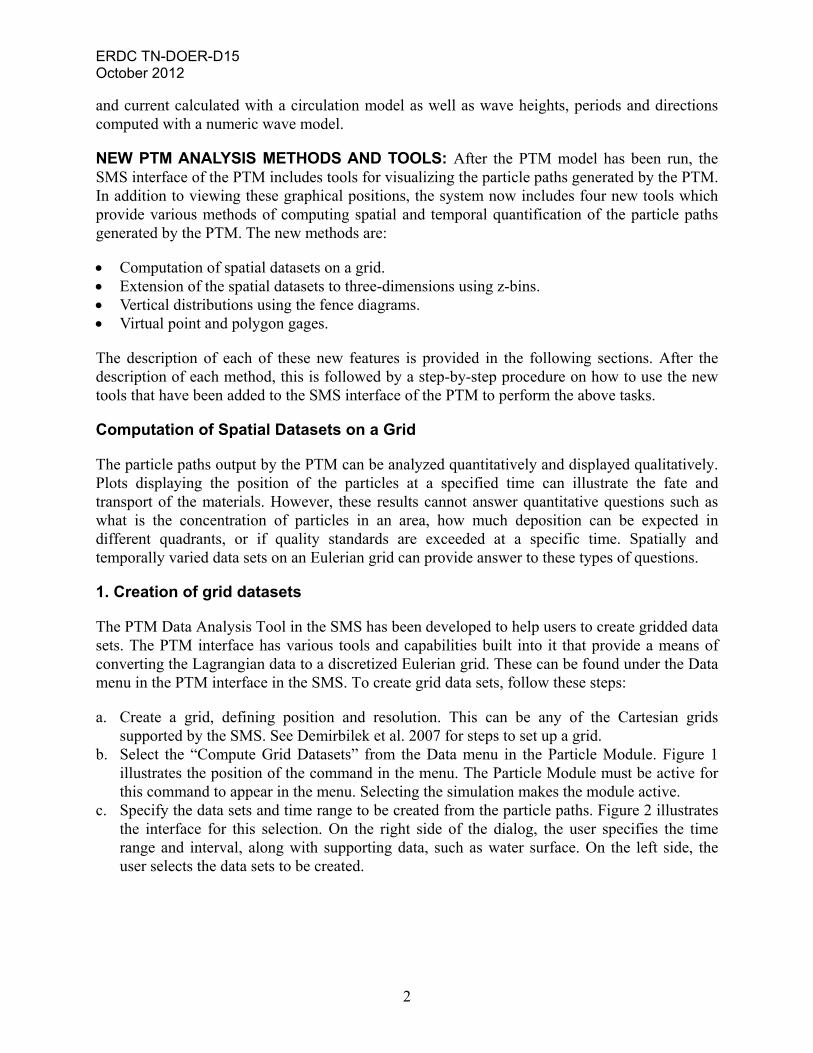
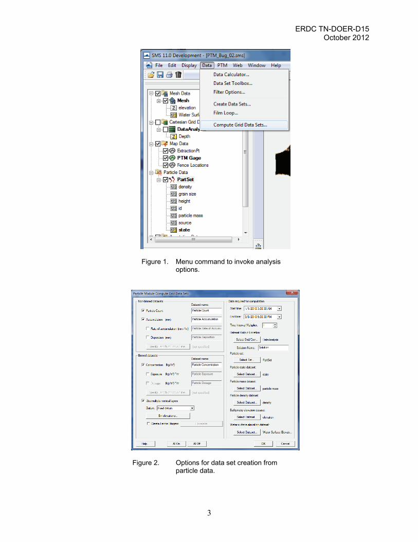
b. Select the “Compute Grid Datasets” from the Data menu in the Particle Module. Figure 1 illustrates the position of the command in the menu. The Particle Module must be active for this command to appear in the menu. Selecting the simulation makes the module active.

c. Specify the data sets and time range to be created from the particle paths. Figure 2 illustrates the interface for this selection. On the right side of the dialog, the user specifies the time range and interval, along with supporting data, such as water surface. On the left side, the user selects the data sets to be created.


3

Figure 1. Menu command to invoke analysis options.

Figure 2. Options for data set creation from particle data.


4

2. Types of grid datasets

The PTM Data Analysis Tool in the Data menu supports the creation of the following grid data sets:

Particle Count: The number of particles in the Cartesian grid cell. Accumulation: The depth of material deposited on the bed in the Cartesian grid cell in the

previous time interval. The volume of particles is calculated using the particle mass and density data set for particles which are deposited on the bed (based on the state data set) and in the cell. The volume in each cell is divided by the area of the cell to calculate an average depth in the cell. No voids ratio is included at this time. However the general “Data Calculator” in the SMS can be used to modify the resulting data set.

Rate of accumulation: The change in accumulation over time. Deposition: The change in depth of particles in the Cartesian grid cell during a user specified

focus time. Concentration: The concentration of particles in the Cartesian grid cell. The volume of

particles is calculated using the particle mass and density data set for particles which are active (based on the state data set) and in the cell. This volume is then divided by the volume of the cell using the specified bathymetry and water surface elevation data sets. The bathymetry and water surface elevation must come from the same geometric object.

Exposure: The cumulative exposure in the Cartesian grid cell. Dosage: The exposure in the Cartesian grid cell during the focus time.

3. Effect of grid resolution

One important factor that must be considered in the creation grid data sets is the grid resolution (the number of cells created within the grid area). When creating a grid data set, the number of cells generated within the gridded domain is determined by the user. The subsequent calculations of particle count, concentration, accumulation, etc will obviously be affected by resolution. The ultimate objective is to select a resolution that is coarse enough so that individual particles entering a cell do not dramatically change the results, but fine enough to resolve the spatial variation of the quantities. Consequently, it is recommended that users perform “sensitivity” tests on grid resolution to make sure the resolution specified by the user is reasonable (MacDonald et al. 2006; Davies et al. 2005; Demirbilek et al. 2005a, 2005b). This subject is further discussed and illustrated in the Part 2 companion Technical Note in an example.

Use of z-Bins to Extend the Spatial Datasets to 3-D

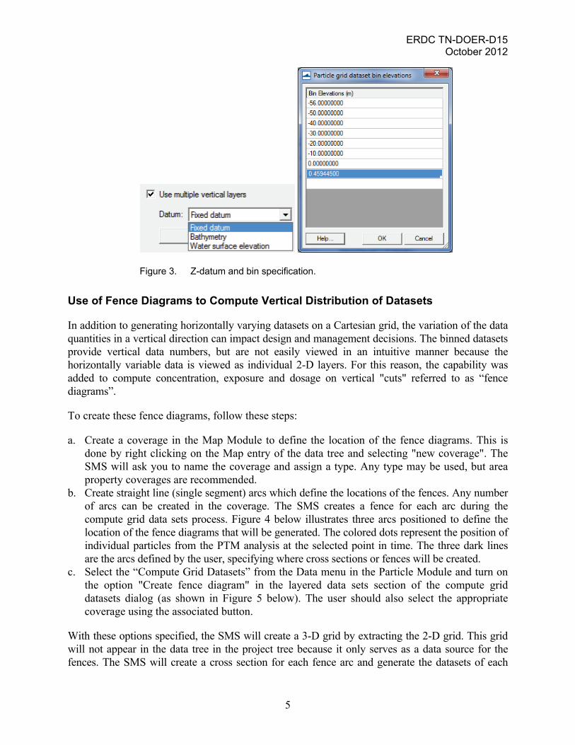
Of the datasets described in the previous section, the concentration, exposure and dosage can be binned based on z-value by clicking the "Use multiple bins" toggle. The datum (fixed, relative to bathymetry or relative to water surface elevation) as shown in Figure 3 below, can be specified by clicking on the "Bin elevations" button that opens the bin elevations dialog to define the bin values. This is illustrated in Part 2 of this Technical Note.


5

Figure 3. Z-datum and bin specification.

Use of Fence Diagrams to Compute Vertical Distribution of Datasets

In addition to generating horizontally varying datasets on a Cartesian grid, the variation of the data quantities in a vertical direction can impact design and management decisions. The binned datasets provide vertical data numbers, but are not easily viewed in an intuitive manner because the horizontally variable data is viewed as individual 2-D layers. For this reason, the capability was added to compute concentration, exposure and dosage on vertical "cuts" referred to as “fence diagrams”.

To create these fence diagrams, follow these steps:

a. Create a coverage in the Map Module to define the location of the fence diagrams. This is done by right clicking on the Map entry of the data tree and selecting "new coverage". The SMS will ask you to name the coverage and assign a type. Any type may be used, but area property coverages are recommended.

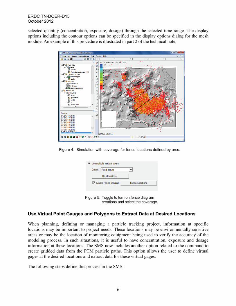
b. Create straight line (single segment) arcs which define the locations of the fences. Any number of arcs can be created in the coverage. The SMS creates a fence for each arc during the compute grid data sets process. Figure 4 below illustrates three arcs positioned to define the location of the fence diagrams that will be generated. The colored dots represent the position of individual particles from the PTM analysis at the selected point in time. The three dark lines are the arcs defined by the user, specifying where cross sections or fences will be created.

c. Select the “Compute Grid Datasets” from the Data menu in the Particle Module and turn on the option "Create fence diagram" in the layered data sets section of the compute grid datasets dialog (as shown in Figure 5 below). The user should also select the appropriate coverage using the associated button.

With these options specified, the SMS will create a 3-D grid by extracting the 2-D grid. This grid will not appear in the data tree in the project tree because it only serves as a data source for the fences. The SMS will create a cross section for each fence arc and generate the datasets of each


6

selected quantity (concentration, exposure, dosage) through the selected time range. The display options including the contour options can be specified in the display options dialog for the mesh module. An example of this procedure is illustrated in part 2 of the technical note.

Figure 4. Simulation with coverage for fence locations defined by arcs.

Figure 5. Toggle to turn on fence diagram creations and select the coverage.

Use Virtual Point Gauges and Polygons to Extract Data at Desired Locations

When planning, defining or managing a particle tracking project, information at specific locations may be important to project needs. These locations may be environmentally sensitive areas or may be the location of monitoring equipment being used to verify the accuracy of the modeling process. In such situations, it is useful to have concentration, exposure and dosage information at these locations. The SMS now includes another option related to the command to create gridded data from the PTM particle paths. This option allows the user to define virtual gages at the desired locations and extract data for these virtual gages.

The following steps define this process in the SMS:


7

a. Create a "PTM Gage" coverage. (This is a new coverage type in the SMS version11.0 or later version.) Do this by right clicking on the Map Data entry of the data tree and selecting the new coverage command. A dialog will appear to allow the user to specify the "PTM Gage" type.

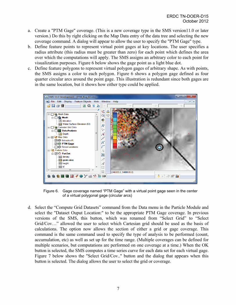
b. Define feature points to represent virtual point gages at key locations. The user specifies a radius attribute (this radius must be greater than zero) for each point which defines the area over which the computations will apply. The SMS assigns an arbitrary color to each point for visualization purposes. Figure 6 below shows the gage point as a light blue dot.

c. Define feature polygons to represent virtual polygon gages of arbitrary shape. As with points, the SMS assigns a color to each polygon. Figure 6 shows a polygon gage defined as four quarter circular arcs around the point gage. This illustration is redundant since both gages are in the same location, but it shows how either type could be applied.

Figure 6. Gage coverage named “PTM Gage” with a virtual point gage seen in the center of a virtual polygonal gage (circular arcs)

d. Select the “Compute Grid Datasets” command from the Data menu in the Particle Module and select the "Dataset Ouput Location:" to be the appropriate PTM Gage coverage. In previous versions of the SMS, this button, which was renamed from “Select Grid” to “Select Grid/Cov…” allowed the user to select which Cartesian grid should be used as the basis of calculations. The option now allows the section of either a grid or gage coverage. This command is the same command used to specify the type of analysis to be performed (count, accumulation, etc) as well as set up for the time range. (Multiple coverages can be defined for multiple scenarios, but computations are performed on one coverage at a time.) When the OK button is selected, the SMS computes a time series curve for each data set for each virtual gage. Figure 7 below shows the "Select Grid/Cov.." button and the dialog that appears when this button is selected. The dialog allows the user to select the grid or coverage.


8

Figure 7. Button to direct output to a virtual gage coverage and the selection window.

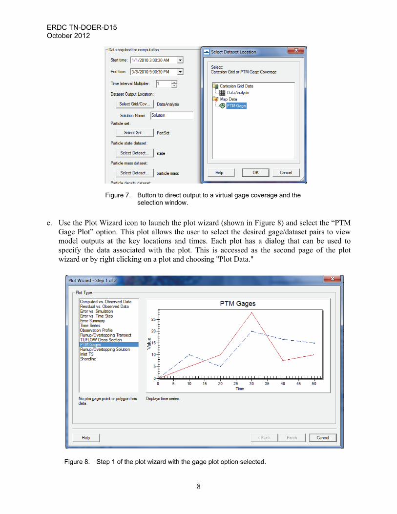
e. Use the Plot Wizard icon to launch the plot wizard (shown in Figure 8) and select the “PTM Gage Plot” option. This plot allows the user to select the desired gage/dataset pairs to view model outputs at the key locations and times. Each plot has a dialog that can be used to specify the data associated with the plot. This is accessed as the second page of the plot wizard or by right clicking on a plot and choosing "Plot Data."

Figure 8. Step 1 of the plot wizard with the gage plot option selected.


9

An individual gage may represent a vertical bin. The Plot Data dialog will allow the user to choose the objects, simulations, and datasets visualized in the plot. For objects, the user selects from the options to "Use Selected Objects" or "Specify Objects". If the Specify Objects option is selected, the SMS displays a list of the points and polygons by type and id (i.e., polygon: 1 or point: 2). For simulations and datasets, the SMS displays a listbox for each type containing all the simulations or datasets with check boxes to select the ones that should be displayed.

CONCLUSIONS: This Technical Note introduces four new data analysis tools developed recently for the PTM and their graphical implementation in the SMS interface. Features of these new data analysis capabilities of PTM are discussed in this user guide. The user-friendly SMS interface allows for efficient production of the PTM data analysis results to predict transport of sediment in open water. Data analysis tools described herein allow users to calculate data sets on a grid, extend data to three dimensions using z-bins, examine vertical distribution by using the fence diagrams, and place virtual gauges at environmentally sensitive locations to calculate particle count, accumulation, rate of accumulation, deposition, concentration, exposure and dosage over a user-specified focus time. A detailed description of these functions is provided in this TN. Step-by-step instructions are provided in the companion Part 2 Technical Note to demonstrate an application of these tools in an example case study.

ADDITIONAL INFORMATION: This Technical Note was written under the Dredging Operations and Environmental Research (DOER) program by Dr. Zeki Demirbilek (Zeki.Demirbilek@ usace.army.mil, Tel: 601-634-2834, Fax: 601-634-3433), and Tahirih Lackey ([email protected]), of the U.S. Army Engineer Research and Development Center (ERDC), Coastal and Hydraulics Laboratory (CHL); and Dr. Alan Zundel (azundel@ aquaveo.com) of the Aquaveo, LLC and Brigham Young University.

This DOER Technical Note should be referenced as follows:

Demirbilek, Z., T.C. Lackey, and A. K. Zundel. 2012. Particle Tracking Model Data Analysis Tools –Part 1: Capabilities in SMS. DOER Technical Notes Collection. ERDC TN-DOER-D15. U.S. Army Engineer R&D Center, Vicksburg, MS.

This DOER-TN and files for the examples may be downloaded from http://chl.wes.army.mil/

library/ publications/chetn/ and http://xmswiki.com/.

REFERENCES

Davies, M., N. MacDonald, Z. Demirbilek, J. Smith, A. Zundel, and R. Jones. 2005. Particle Tracking Model (PTM) in the SMS: II. Overview of features and capabilities. Dredging Operations and Environmental Research Technical Note Collection (ERDC-TN-DOER-D5), U.S. Army Engineer Research and Development Center, Vicksburg, MS.

Demirbilek, Z., T. Lackey, and A. Zundel. 2012. Particle Tracking Model Data Analysis Tools in the SMS -- Part 2: Case Study. Coastal Hydraulic Laboratory Technical Note (ERDC TN-DOER-D16), U.S. Army Engineer Research and Development Center, Vicksburg, MS.

Demirbilek, Z., J. Smith, A. Zundel, R. Jones, N. MacDonald, and M. Davies. 2005a. Particle Tracking Model (PTM) in the SMS: I. Graphical interface. Dredging Operations and Environmental Research Technical Note Collection (ERDC-TN-DOER-D4), U.S. Army Engineer Research and Development Center, Vicksburg, MS.


10

Demirbilek, Z., J. Smith, A. Zundel, R. Jones, N., MacDonald, and M. Davies. 2005b. Particle Tracking Model (PTM) in the SMS: III. Tutorial with examples. Dredging Operations and Environmental Research Technical Note Collection (ERDC-TN-DOER-D6), U.S. Army Engineer Research and Development Center, Vicksburg, MS.

Jones, N. L., R. D. Jones, C. D. Butler, and R. M. Wallace. 2004. A generic format for multi-dimensional models. Proceedings World Water and Environmental Resources Congress 2004. (http://www.pubs.asce.org/ WWWdisplay.cgi?0410405).

MacDonald, N. J., M. H. Davies, A. K. Zundel, J. D. Howlett, T. C. Lackey, Z. Demirbilek, and J. Z. Gailani. 2006. PTM: Particle Tracking Model, Report 1: Model theory, implementation, and example applications. Coastal and Hydraulics Laboratory Technical Report ERDC/CHL TR-06-20, U.S. Army Engineer Research and Development Center, Vicksburg, MS.

Zundel, A. K. 2011. Surface-water modeling system reference manual, Version 11.0. Provo, UT: Aquaveo, LLC, (http://aquaveo.com).

NOTE: The contents of this technical note are not to be used for advertising, publication, or promotional purposes. Citation of trade names does not constitute an official endorsement or approval of the use of such products.

particle tracking model data analysis tools – part 1 ... · particle tracking model data analysis...

Documents