particle swarm optimization for hydraulic analysis of … · 2018-06-03 · particle swarm...
TRANSCRIPT
Civil Engineering Infrastructures Journal, 48(1): 9-22, June 2015
ISSN: 2322-2093
9
Particle Swarm Optimization for Hydraulic Analysis of Water Distribution
Systems
Moosavian, N.1*
and Jaefarzadeh, M.R.2
1 Lecturer, Civil Engineering Department, University of Torbat-e-Heydarieh,
Torbat-e-Heydarieh, Iran 2 Professor, Civil Engineering Department, Ferdowsi University of Mashhad, Mashhad, Iran
Received: 01 Jul. 2013 Revised: 04 Sep. 2014 Accepted: 24 Oct. 2014
Abstract: The analysis of flow in water-distribution networks with several pumps by the Content Model may be turned into a non-convex optimization uncertain problem with multiple solutions. Newton-based methods such as GGA are not able to capture a global optimum in these situations. On the other hand, evolutionary methods designed to use the population of individuals may find a global solution even for such an uncertain problem. In the present paper, the Content Model is minimized using the particle-swarm optimization (PSO) technique. This is a population-based iterative evolutionary algorithm, applied for non-linear and non-convex optimization problems. The penalty-function method is used to convert the constrained problem into an unconstrained one. Both the PSO and GGA algorithms are applied to analyse two sample examples. It is revealed that while GGA demonstrates better performance in convex problems, PSO is more successful in non-convex networks. By increasing the penalty-function coefficient the accuracy of the solution may be improved considerably.
Keywords: Content Model, Global Gradient Algorithm, Hydraulic Analysis, Particle-Swarm Optimization, Water Distribution Systems
INTRODUCTION
In a water distribution network (WDN)
flow rates and nodal heads are computed
by solving a mixture system of linear
(continuity) and nonlinear (energy)
equations. Since 1936 various methods
have been devised for WDN analysis that
directly solve the system equations, e.g.,
the Hardy Cross method (Cross, 1936), the
Newton-Raphson method (Martin and
Peters, 1963; Shamir and Howard, 1968),
and the linear theory method (Wood and
Charles, 1972). However, Collins et al.
(1978) proposed a mathematical
optimization technique, the so-called
Content Model, that minimized a nonlinear
*Corresponding author Email: [email protected]
convex objective function subject to a set
of linear equality constraints. The
convexity of the objective function
guaranteed the existence and uniqueness of
the solution. However, the nonlinear
programming methods used for the
solution of the Content Model were time-
consuming, reducing the practical
application of the model in large complex
networks. Todini and Pilati (1988)
developed a Newton-based global gradient
algorithm (GGA), originally based on the
minimization of a slightly modified
Content Model. Basically, GGA involves
two iterative steps, where the heads and
flows are obtained, respectively (Elhay and
Simpson, 2011). Simpson (2010)
compared Q-equations and GGA

Moosavian, N. and Jaefarzadeh, M.R.
10
formulation in analyzing water distribution
systems. Todini and Rossman (2013)
introduced a unified framework for
deriving simultaneous equation algorithms
for WDNs. Moosavian and Jaefarzadeh
(2014) applied an efficient higher-order
method and reduced the number of
iterations of the Hardy Cross algorithm.
Recently, some innovative techniques have
been developed for simplifying the
topological representation of pipe
networks while preserving the accuracy of
the analysis (see for example Giustolisi,
2010; Giustolisi et al., 2012).
In a pipe network problem quite a few
pumps may be provided externally to
supply water from reservoirs, or internally
within the network as booster pumps to
augment pressure and discharge
accordingly at certain locations within the
system. At a constant rotational speed, there
is a unique relationship between the
delivered head hp and supplied discharge Q,
known as the pump head-discharge curve.
The head-discharge curves for various
kinds of pump are different. Usually in
screw pumps these curves are stable and
strictly monotonically decreasing, i.e., the
head decreases as the flow rate increases.
Thus, for a given head there is only one
value for the flow rate. However, for some
centrifugal and half-axial pumps, the
characteristic head-discharge curve is
unstable or not continuously decreasing as
the flow rate increases. In other words, for
the same head, two or three discharges may
exist (Bhave and Gupta, 2006). The
analysis of a distribution network with
several pumps with unstable or in some
cases even stable head-discharge curves is a
non-convex uncertain problem with
multiple solutions as operating points.
Generally, the convergence characteristics
of the Newton-type methods such as GGA
are highly sensitive to the initial guesses of
the solution. Specifically in non-convex
problems, these methods will fail if the
initial guesses are not sufficiently close to
the global minimum (Luenberger and
Yinyu, 2008). In other words, they may trap
into a local minimum, leading to the wrong
solution.
On the other hand, evolutionary methods
are intrinsically designed to find a global
solution even in uncertain problems. Over
the last two decades many evolutionary
techniques have been successfully applied
to minimize the cost function of pipes. This
is a non-convex function with discrete
decision variables. The most important
techniques include genetic algorithms
(Murphy and Simpson,1992; Simpson et
al., 1994; Dandy et al.,1996; Savic and
Walters, 1997); simulated annealing (Cunha
and Sousa, 2001); harmony search (Geem,
2006); the shuffled frog-leaping algorithm
(Eusuff and Lansey, 2003); ant-colony
optimization (Maier et al., 2003); particle-
swarm optimization (Suribabu and
Neelakantan, 2006); cross entropy
(Perelman and Ostfeld, 2007); scatter
search (Lin et al., 2007); differential
evolution (Suribabu, 2010) and Vasan and
Simonovic, 2010); self-adaptive differential
evolution (Zheng et al., 2013) and the
soccer-league competition algorithm
(Moosavian and Kasaee, 2014). Moosavian
and Jaefarzadeh (2014) applied a shuffled
complex-evolution technique (SCE) in a
head-based optimization model (Co-
Content Model) for the hydraulic analysis
of pipe networks. This methodology was
able to accurately simulate pressure-driven
demand and leakage in pipe networks.
In this article the Content Model is
optimized using an evolutionary-type
algorithm called particle swarm
optimization (PSO). In this methodology,
there is no need to solve a system of linear
or non-linear equations where a proper
initial solution vector is crucial to the
convergence of non-convex problems.

Civil Engineering Infrastructures Journal, 48(1): 9-22, June 2015
11
CONTENT MODEL APPROACH
As mentioned, the solution of the content-
optimization model by Collins et al. (1978)
yielded the network analysis. A simplified
version of this model is presented herein
by applying it to the one-loop network
shown in Figure 1, where nodes 1 and 2
are source nodes with known head values
H1, and H2, and nodes 3, 4 and 5 are
known demand nodes q3, q4 and q5. Let
pipes 1 to 5 have the known resistances R1
to R5, respectively. The Content Model
aims to minimize the energy function C(Q)
(Bhave and Gupta, 2006):
1 2
n 1 n 1
1 1 2 2
n 1 n 1
3 3 4 4
n 1
5 5 1 2
C(Q) R Q n 1 R Q n 1
R Q n 1 R Q n 1
R Q n 1 Q H Q H
(1)
This is subject to the following node-
flow continuity constraints:
0qQQQ
0qQQ
0qQQQ
5324
435
3451
(2)
The objective function (1) contains
integral functions of the head loss terms in
pipes 1 to 5 and potential energy terms in
source nodes 1 and 2, respectively. Note
that the node-flow continuity constraints
should be written for all nodes of the
network with unknown heads. Since all
node-flow continuity constraints and loop-
head loss equations have to be satisfied,
the solution of the optimization model
gives the discharges in the pipes, hence the
network analysis. If there is a pump, for
example in pipe (2), with a head-discharge
curve approximated by a quadratic
equation hp= AQ2+BQ+C, the energy
function model may be modified
accordingly:
1 2
n 1 n 1
1 1 2 2
n 1 n 1
3 3 4 4
n 1
5 5 1 2
3 2
2 2 2
C(Q) R Q n 1 R Q n 1
R Q n 1 R Q n 1
R Q n 1 Q H Q H
(A Q 3 B Q 2 C Q )
(3)
where A, B and C: are constant
coefficients. The Content Model in a
general form may be expressed as:
Minimize :n 1
j j k k
j k
3 2
l l l
l
C(Q) R Q n 1 Q H
A Q 3 B Q 2 C Q
j pipe, k source node, l pump
(4.1)
Subject to
j i
j
:
Q q 0, for all i (4.2)
Note that the second summation in the
objective function is only for source nodes
with known heads, while the constraints
are written for nodes with unknown heads.
In the global gradient algorithm presented
by Todini and Pilati (1987), the optimization
model of (4.1) and (4.2) is unconstrained by
a number of Lagrange Multipliers, and the
resulting equations are solved by the
Newton-Raphson method. Thereby, the
estimates for Q and H are updated at each
iteration directly. The convergence rate of
this algorithm may be of the second order,
provided that initial guesses are sufficiently
close to the final solution (Luenberger,
Yinyu, 2008). At present, GGA is applied
for water distribution network analysis in
commercial and industrial software such as
WaterGEMS and EPANET (Rossman,
2002).

Moosavian, N. and Jaefarzadeh, M.R.
12
Fig. 1. Schematic representation of the looped pipe network with 5 pipes.
On The Convexity Property of the
Content Model
If an optimization model is convex,
Newton-based methods can easily
minimize it with any arbitrary initial guess,
and the existence and uniqueness of the
solution are guaranteed. However, for non-
convex functions with several optima,
these methods may not necessarily capture
a global optimum. Instead, they are likely
to be trapped in a local optimum,
depending on initial guesses at the
beginning of the solution process.
On the other hand, meta-heuristic
algorithms examine the whole domain of
the problem as much as possible and seek
a global optimum independent of the initial
guesses. To illustrate the convexity
behaviour of the Content Model in the
presence or absence of a pump, consider
the network shown in Figure 2, including
one reservoir, two nodes and three pipes.
The Content Model may be written as:
1 1
Minimize : n 1
1 1
n 1 n 1
2 2 3 3
1 2
C(Q) R Q n 1
R Q n 1 R Q n 1
Q H Q H
(5.1)
Subject to :
1 3 2
2 3 1
Q Q q 0
Q Q q 0
(5.2)
In Eq. (5.1) the absolute values are
removed, presuming the flow in the pipes
is selected in proper directions.
Substituting for Q2 and Q3 from constraints
(5.2) into (5.1), the Content Model may be
modified as:
(6)
Minimize : n 1
1 1
n 1
2 1 2 1
n 1
3 1 2
1 1 1 2 1 1
C(Q) R Q n 1
R Q q q n 1
R Q q n 1
Q H Q q q H
The second derivative of Equation (6)
yields a positive function:
(7)
0
2n 1n 1
1 1 2 1 2 12
1
n 1 n 1
3 1 2 1 1
n 1 n 1
2 2 3 3
CnR Q nR Q q q
Q
nR Q q nR Q
nR Q nR Q
The positiveness of Eq. (7) assures the
convexity of the Content Model and GGA
is therefore able to find the proper
solution. When two pumps are placed in
pipes 1 and 2, the Content Model is
modified as:

Civil Engineering Infrastructures Journal, 48(1): 9-22, June 2015
13
(8)
Minimize :n 1 n 1n 1
1 1 2 1 2 1 3 1 2
3 23 2
1 1 1 1 1 1 2 1 2 1 2 1 2 1
2 1 2 1 1 1 1 2 1 1
C(Q) R Q n 1 R Q q q n 1 R Q q n 1
A Q 3 B Q 2 C Q A Q q q 3 B Q q q 2
C Q q q Q H Q q q H
The second derivative of Eq. (8) gives:
(9)
222111
1n
33
1n
22
1n
11
21212111
1n
213
1n
1212
1n
112
2
BQ2ABQ2AQnRQnRQnR
BqqQ2ABQ2A
qQnRqqQnRQnRQ
C
In this case, Eq. (9) may not be positive
for some values of A and B; even for a
strictly monotonically decreasing head-
discharge curve, the Content Model is non-
convex. As an example, for typical values
of constant coefficients, consider the
sample energy curve in Figure 3 for the
one-looped pipe network shown in Figure
2. The Content Model has two minima;
however, GGA is able to find only one
local solution depending on the selection
of initial guesses. This solution may not
necessarily be a global optimum.
Evolutionary methods are to be used to
resolve this problem and to find the global
minimum. In the following, a powerful
evolutionary approach for minimizing the
Content Model will be introduced.
Fig. 2. Schematic representation of the looped pipe network with three pipes.

Moosavian, N. and Jaefarzadeh, M.R.
14
-1 -0.5 0 0.5 1 1.5-200
-100
0
100
200
300
400
500
600
Discharge (Q)
C(Q
)
Fig. 3. System energy curve for one- looped pipe network.
PARTICLE SWARM OPTIMIZATION
Particle swarm optimization (PSO) is an
adaptive evolutionary algorithm based on
population search (Kennedy and Eberhart,
1995). It is a simple and fast converging
technique simulating the social behaviour
of birds flocking and fish schooling.
Consider a swarm of flying birds looking
for a piece of food (global optimum) in an
area. No bird in the group knows the exact
location of the food, but they may identify
the one closest to the food, and obviously
their best choice is to follow that bird (Zhu
et al., 2011). In PSO each solution is taken
as a bird in the group or a particle in the
swarm, having a certain position and
velocity, but with zero mass. The location
and velocity of the particles are updated in
consecutive iterations. The various steps in
this algorithm may be classified as follows.
Step 1: Define the optimization problem
and constraints
The optimization problem together with
its constraints (if any) are specified as:
Subject to :
Minimize : i
i
C( )
0
X
h(X ) (10)
where C(Xi): is an objective function, Xi: is
the set of decision variables for particle i
and h(Xi): is the set of constraints. PSO is
basically an unconstrained algorithm but
may be used for constrained problems as
well with a penalty function, as will be
explained later.
Step 2: Generate samples
Each particle i is associated with three
vectors: 1. The particle’s current position
iNi2i1i x,...,x,xX
where N: is the number of
decision variables;
(11)
2. The best location it has reached so far
iNi2i1i pbest,...,pbest,pbestbest P (12)
3. Its current velocity, which enables it to evolve
to a new position
iNi2i1i v,...,v,vV (13)
The initial population of the PSO may
be created arbitrarily by
imaximiniimini XXτXX (14)
where τi: denotes a uniformly distributed
random vector within the range of [0,1],
and iminX and imaxX : are the maximum and
minimum bounds of particle i. Then, the
objective functions (Ci(Xi), i= 1, …, nPop)
of all the individuals in the population are
Discharge-Q (m3/s)
C(Q
)-(m
4/s
)
Civil Engineering Infrastructures Journal, 48(1): 9-22, June 2015
15
calculated. The position matrix of the
population of generation G may be
represented as:
(15) ( )
1 1 2 2, ,G
nPop nPopP C C C
X X X
where nPop: is the number of populations.
Step 3: Start the iterative process
In this step, the best position that every
particle has reached so far (Pbest) is found
and the best Pbest is set as the best global
position (Gbest). Then, two main steps of
PSO are performed sequentially to create
the new solution vectors.
Step 3.1: Update velocities
The new velocity, Vi, may be obtained
as follows:
i i 1 i i i
2 i i
ω c best
c best
V V P X
G X
(16)
where Gbest: is the best position vector
attained by any particle during the
optimization process, c1 and c2: are the
acceleration constants, representing the
weights of the stochastic acceleration
terms that respectively pull each particle
simultaneously towards its best position
and the best global position, αi and βi: are
constant functions, generating uniform
pseudo-random numbers between 0 and 1
(sometimes referred to as learning rates or
factors), and ω: is an inertia term proposed
by Shi and Eberhart (1998), which controls
the impact of the velocity history into the
new velocity and provides improved
performance in a number of applications.
This last parameter may be suitably
adapted during the calculation process.
The operation (16) allows a balance
between the local and global search.
Step 3.2: Update particles’ positions
The particles’ positions are updated
accordingly as follows:
iii XVX (17)
Step 4: Check the stopping criterion
The steps 3.1 and 3.2 are repeated until a
termination criterion is satisfied. This
condition may be stated either in terms of a
maximum number of iterations or a certain
value for the objective function.
Penalty Function
The PSO algorithm is designed for
unconstrained optimization models. The
penalty function method may be used for
changing constrained models into
unconstrained ones (Luenberger and
Yinyu, 2008). A penalty function is
defined as the summation of square
constraints:
m
1j
2
ijP )(Xh)(X i (18)
where m: is the number of constraints. An
unconstrained model is then obtained by
adding the penalty function to the
objective function:
Minimize :
i 1,nPop
C( ) μP
i iX (X ) (19)
where μ: is a large positive constant
coefficient.
Implementation of PSO in Pipe Network
Analysis Pipe-network analysis in Content
Model, i.e., as in Eqs. (4.1) and (4.2), is a
constrained optimization problem. To
eliminate the constraints this model may
be treated by a penalty function similar to
Eq. (19). The PSO algorithm may then be
used to minimize Eq. (19), where decision
variables are flow-rate in pipes with a
maximum bound set to the sum of all
demands and a minimum bound of zero.
Both the PSO and GGA algorithms are
applied to analyse two network problems
in this section. The residuals of node -
balance summed up over all nodes and the
residuals of loop energy balance summed

Moosavian, N. and Jaefarzadeh, M.R.
16
up over the loops are calculated to examine
the accuracy of solutions. All of the
computations were executed in a
MATLAB environment with an Intel(R)
Core(TM) 2Duo CPU P8700 with
2.53GHz and 4.00 GB RAM.
NUMERICAL EXAMPLE 1
Consider a three-loop network with 5 nodes
and 7 pipes, where the node-, pipe- and loop-
numbers are shown in Figure 4 as reported
by Todini (2006). The pipes’ resistances are
R1=1.5625, R2=50, R3=100, R4=12.5,
R5=75, R6=200, and R7=100, respectively.
The algorithms of PSO, minimizing the
Content Model plus penalty functions and
GGA by applying Newton-Raphson iterative
method are applied to analyse this network.
Each of these algorithms was tested 100
times with different initial guesses. The
selected parameters for the implementation
of the PSO algorithm included: number of
decision variables = 7; population = 700
(100 times the number of decision
variables); and number of iterations = 300.
Based on the authors’ experience, if the
population is selected as 100 times the
decision variables, the algorithm
performance will be efficient in all runs. The
decision variables were set between a lower
bound of 0 and an upper bound of 1 m3/s,
equal to the sum of demands in all nodes.
The convergence properties of objective
function evaluation and the total mass and
energy balances against the number of
iterations for the PSO method are shown in
Figures 5 and 6 for the two penalty-function
coefficients μ=106 and μ=10
9, respectively.
The accuracy of mass balance increases the
larger the value of μ. The objective function
was evaluated for 100 runs of the GGA and
PSO methods. In Table 1, the best, worst,
average and standard deviation of the
solutions obtained from the different runs
indicate that both methods generate similar
results. However, in Table 2 the mass
balance at nodes and the energy balance
around the loops reveal that GGA produces
more accurate results than PSO. This is due
to the convexity of the Content Model in the
absence of any pump in the system, where
the Newton-based models are highly
successful in detecting the global optimum
solution.
Fig. 4. Schematic representation of the three-looped pipe network (Todini, 2006).

Civil Engineering Infrastructures Journal, 48(1): 9-22, June 2015
17
Table 1. Evaluation of objective function in PSO and GGA for example 1(μ=109).
Best Worst Mean Std
PSO -99 -99 -99 1.57e-014
GGA -99 -99 -99 7.03E-13
Table 2. Evaluation of mass and energy balance in PSO and GGA for Example 1 (μ=109).
Mass Balance (Node) PSO GGA Energy Balance (Loop) PSO GGA
1 4.95E-8 -3.47E-15 123 -3.42E-08 2.22E-16
2 4.90E-8 1.72E-15 356 7.56E-07 4.44E-16
3 4.85E-8 8.88E-16 457 -6.16E-07 -1.11E-16
4 4.80E-8 2.83E-15
0 20 40 60 80 100 120 140 160 180 20010
-10
10-5
100
105
1010
Number of Iterations
Energy Balance
Mass Balance
Function Evaluation
Fig. 5. Mass and energy balances and function evaluation versus the number of iterations for the PSO algorithm
with μ=106, Example 1.
0 20 40 60 80 100 120 140 160 180 20010
-10
10-5
100
105
1010
Number of Iterations
Energy Balance
Mass Balance
Function Evaluation
Fig. 6. Mass and energy balances and function evaluation versus the number of iterations for the PSO algorithm
with μ=109, Example 1.
En
erg
y B
ala
nce
-Mass B
ala
nce
- F
unctio
n E
va
lua
tion
E
ne
rgy B
ala
nce
-Mass B
ala
nce
- F
unctio
n E
va
lua
tion
Moosavian, N. and Jaefarzadeh, M.R.
18
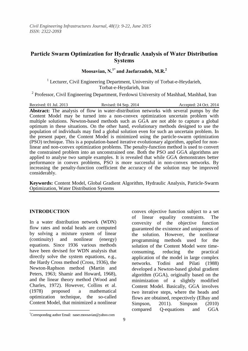
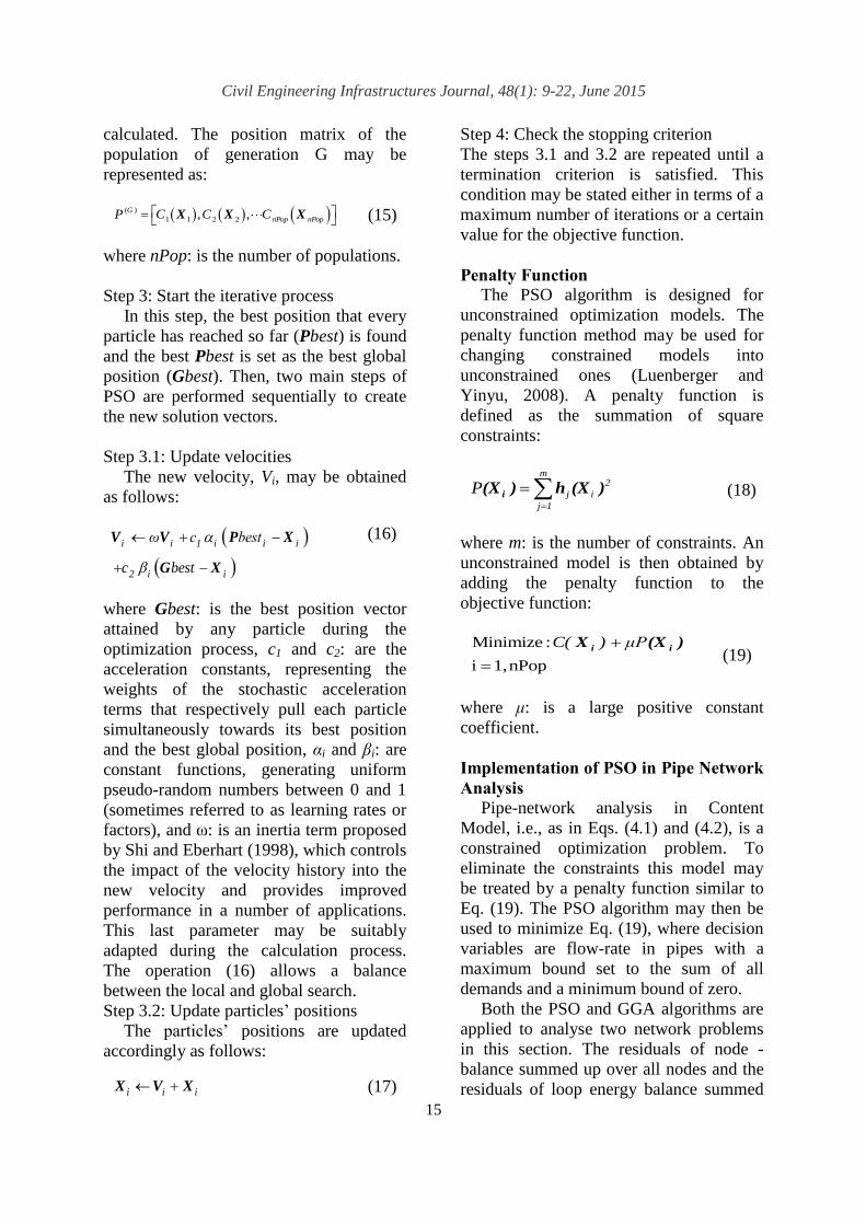
NUMERICAL EXAMPLE 2
Consider the eight-pipe network shown in
Figure 7, including two reservoirs, a source
pump that supplies some of the system
demand, and a booster pump placed in pipe
1. There are two globe valves, which have a
loss coefficient of 10, in pipes 7 and 8, and
two of the meter in pipe 3 (Larock et al.,
2000). The pipes’ resistances are R1=1160,
R2=613, R3=1160, R4=690, R5=1292,
R6=1115, R7=322 and R8=239,
respectively, and the pumps’ characteristic
curves are approximated by hp1 = -
2220Q2+44.4Q+12.28 and hp2 = -
55.6Q2+1.667Q+4.1. In a similar manner
to Example 1, this network was analysed
100 times with different initial guesses
using the two methods of GGA and PSO.
The parameters selected for the PSO model
included: number of decision variables = 8;
population = 800 (100 times the number of
decision variables); and number of
iterations = 500. The range of initial
guesses was between 0.0 and 0.24 m3/s. In
Table 3, the best, worst, average and
standard deviation of the objective function,
obtained from 100 runs with different initial
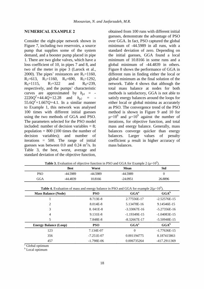
guesses, demonstrate the advantage of PSO
over GGA. In fact, PSO captured the global
minimum of -44.5989 in all runs, with a
standard deviation of zero. Depending on
the initial guesses, GGA found a local
minimum of 10.8166 in some runs and a
global minimum of -44.4839 in others.
Figure 8 shows the performance of GGA in
different runs in finding either the local or
global minimum as the final solution of the
network. Table 4 shows that although the
total mass balance at nodes for both
methods is satisfactory, GGA is not able to
satisfy energy balances around the loops for
either local or global minima as accurately
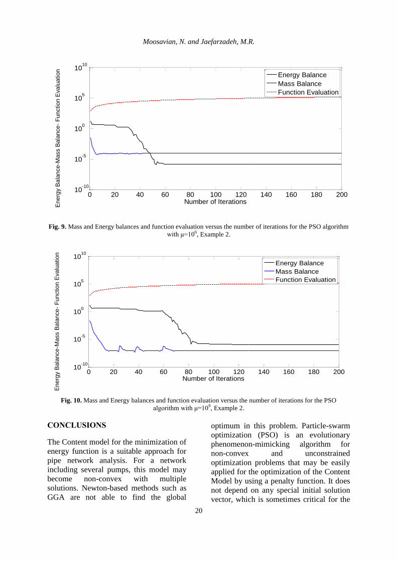
as PSO. The convergence trend of the PSO
method is shown in Figure 9 and 10 for
μ=106 and μ=10
9 against the number of
iterations, for objective function, and total
mass and energy balance. Generally, mass
balances converge quicker than energy
balances. Larger values of penalty
coefficient μ result in higher accuracy of
mass balances.
Table 3. Evaluation of objective function in PSO and GGA for Example 2 (μ=109).
Best Worst Mean Std
PSO -44.5989 -44.5989 -44.5989 0
GGA -44.4839 10.8166 -24.0951 26.8896
Table 4. Evaluation of mass and energy balance in PSO and GGA for example 2(μ=10
9).
Mass Balance (Node) PSO GGAa
GGAb
1 8.713E-8 2.77556E-17 -2.52576E-15
2 8.014E-8 5.13478E-16 9.14546E-15
3 8. 041E-8 -3.33067E-16 -5.27356E-16
4 9.131E-8 -1.19349E-15 -1.04083E-15
5 7.848E-8 -8.32667E-17 -5.50948E-15
Energy Balance (Loop) PSO GGAa
GGAb
123 7.134E-07 0 -1.77636E-15
356 -7.251E-07 0.001194775 8.187415863
457 -1.798E-06 0.006735264 -417.2911369 a Global optimum
b Local optimum
Civil Engineering Infrastructures Journal, 48(1): 9-22, June 2015
19
Fig. 7. Schematic representation of the looped pipe network for Example 2, (Larock et al., 2000).
Fig. 8. Performance of GGA in finding local or global minimum for 100 different runs.
Number of Runs
Moosavian, N. and Jaefarzadeh, M.R.
20
0 20 40 60 80 100 120 140 160 180 20010
-10
10-5
100
105
1010
Number of Iterations
Energy Balance
Mass Balance
Function Evaluation
Fig. 9. Mass and Energy balances and function evaluation versus the number of iterations for the PSO algorithm
with μ=106, Example 2.
0 20 40 60 80 100 120 140 160 180 20010
-10
10-5
100
105
1010
Number of Iterations
Energy Balance
Mass Balance
Function Evaluation
Fig. 10. Mass and Energy balances and function evaluation versus the number of iterations for the PSO
algorithm with μ=109, Example 2.
CONCLUSIONS
The Content model for the minimization of
energy function is a suitable approach for
pipe network analysis. For a network
including several pumps, this model may
become non-convex with multiple
solutions. Newton-based methods such as
GGA are not able to find the global
optimum in this problem. Particle-swarm
optimization (PSO) is an evolutionary
phenomenon-mimicking algorithm for
non-convex and unconstrained
optimization problems that may be easily
applied for the optimization of the Content
Model by using a penalty function. It does
not depend on any special initial solution
vector, which is sometimes critical for the
En
erg
y B
ala
nce
-Mass B
ala
nce
- F
unctio
n E
va
lua
tion
En
erg
y B
ala
nce
-Mass B
ala
nce
- F
unctio
n E
va
lua
tion

Civil Engineering Infrastructures Journal, 48(1): 9-22, June 2015
21
convergence of Newton-based methods.
There is no need to solve linear systems of
equations during the solution process and
hence no need for huge memories. It has
been shown that by enhancing the penalty
function coefficient the accuracy of the
solution may be improved considerably.
REFERENCES Bhave, P.R. and Gupta, R. (2006). Analysis of
water distribution networks, Alpha Science
International Ltd, Oxford, U.K, 278-285, India.
Collins, M.A., Cooper, L.R. Helgason.,
Kennington, J. and Leblanc, L. (1978). “Solving
the pipe network analysis problem using
optimization techniques”, Management Science,
24(7), 747-760.
Cross, H. (1936). “Analysis of flow in networks of
conduits or conductors”, No. 286, University of
Illinois, Engineering Experimental Station,
Urbana, Illinois, Bulletin.
Cunha, M.C. and Sousa, J. (2001). “Hydraulic
infrastructures design using simulated
annealing”, Journal of Infrastructure Systems,
7(1), 32–38.
Dandy, G.C., Simpson, A.R. and Murphy, L.J.
(1996). “An improved genetic algorithm for
pipe network optimization”, Water Resources
Research, 32(2), 449–457.
Elhay, S. and Simpson, A.R. (2011). “Dealing with
zero flows in solving the nonlinear equations for
water distribution systems”, Journal of
Hydraulic Engineering, ASCE, 137(10), 1216-
1224.
Eusuff, M.M. and Lansey, K.E. (2003).
“Optimization of water distribution network
design using shuffled frog leaping algorithm”,
Journal of Water Resources Planning and
Management, 129(3), 210–225.
Geem, Z.W. (2006). “Optimal cost design of water
distribution networks using Harmony Search”,
Engineering Optimization, 38(3), 259-280.
Giustolisi, O., Laucelli, D., Berardi, L. and Savić,
D.A. (2012). “A computationally efficient
modeling method for large size water network
analysis”, Journal of Hydraulic Engineering,
138(4), 313 – 326.
Giustolisi, O. (2010). “Considering actual pipe
connections in WDN analysis”, Journal of
Hydraulic Engineering, 136(11), 889 – 900.
Hall, M.A. (1976). “Hydraulic network analysis
using (Generalized) Geometric Programming”,
Networks, 6(2), 105-130.
Kennedy, J. and Eberhart, R.C. (1995). “Particle
swarm optimization”, In: IEEE International
Conference on Neural Networks, Perth,
Australia, 1942–1948.
Larock, B.E., Jeppson, R. W. and Watters, G.Z.
(2000). Hydraulics of pipeline systems, Boca
Raton, London, New York, Washington D.C.
Lin, M.D., Liu, Y.H., Liu, G.F. and Chu, C.W.
(2007). “Scatter search heuristic for least-cost
design of water distribution networks”,
Engineering Optimization, 39(7), 857–876.
Luenberger, D.G. and Yinyu, Y. (2008). Linear and
nonlinear programming, International Series In
Operations Research and Management Science,
Stanford University.
Maier, H.R., Simpson, A.R., Zecchin, A.C., Foong,
W.K., Phang, K.Y., Seah, H.Y. and Tan, C.L.
(2003). “Ant colony optimization for the design
of water distribution systems”, Journal of Water
Resources Planning and Management, 129(3),
200–209.
Moosavian, N. and Kasaee Roodsari, B. (2014).
“Soccer league competition algorithm: A novel
meta-heuristic algorithm for optimal design of
water distribution networks”, Swarm and
Evolutionary Computation, 17(2), 14-24.
Moosavian, N. and Jaefarzadeh, M. R. (2014).
“Hydraulic analysis of water distribution
network using Shuffled Complex Evolution”,
Journal of Fluids, 20(14), 1-12.
Moosavian, N. and Jaefarzadeh, M. R. (2014).
“Hydraulic analysis of water supply networks
using a Modified Hardy Cross method”,
International Journal of Engineering,
Transactions C, 27(9), 1331-1338.
Murphy, L. J. and Simpson, A. R. (1992). Pipe
optimization using genetic algorithms, Research
Report No. R93, Department of Civil
Engineering, University of Adelaide, Adelaide,
Australia.
Martin, D.W. and Peters, G. (1963). “The
application of Newton's method to network
analysis by digital computer”, Journal of
Institution of Water Engineers and
Scientists,17, 115-129.
Millonas, M.M. (1994). “Swarms, phase transition,
and collective intelligence”, In: C.G. Langton
(ed.), Artificial Life III, Addison Wesley,
Massachusetts, 417–445.
Perelman, L. and Ostfeld, A. (2007). “An adaptive
heuristic cross-entropy algorithm for optimal
design of water distribution systems”,
Engineering Optimization, 39(4), 413–428.
Rossman L. A. (2002). EPANET2 users manual,
Water Supply and Water Resources Division,
National Risk Management Research
Laboratory, Cincinnati, OH45268.
Savic, D.A. and Waters, G.A. (1997). “Genetic
algorithms for least-cost design of water
distribution networks”, Journal of Water
Moosavian, N. and Jaefarzadeh, M.R.
22
Resources Planning and Management, 123(2),
67–77.
Shamir, U. and Howard, C.D. (1968). “Water
distribution systems analysis”, Journal of the
Hydraulics Division, ASCE, 94(HY1), 219-
234.
Shi, Y.F. and Eberhart, R.C. (1998). Parameter
selection in particle swarm optimization, Book
Section, Evolutionary Programming VII,
Lecture Notes in Computer Science, Springer
Berlin Heidelberg, 591–600.
Simpson, A.R., Dandy, G.C. and Murphy, L.J.
(1994). “Genetic algorithms compared to other
techniques for pipe optimization”, Journal of
Water Resources Planning and Management,
120(4), 423–443.
Simpson A.R. (2011) “Comparing the Q-equations
and Todini-Pilati formulation for solving the
water distribution system equations”, Water
Distribution Systems Analysis, 2010, ASCE, 37-
54.
Suribabu, C.R. and Neelakantan, T.R. (2006).
“Design of water distribution networks using
particle swarm optimization”, Urban Water
Journal, 3(2), 111–120.
Suribabu, C. R. (2010). “Differential evolution
algorithm for optimal design of water
distribution networks”, Journal of
Hydroinformatics, 12(1), 66–82.
Todini, E. and Pilati, S. (1988). “A Gradient
Algorithm for the analysis of pipe networks”,
International Conference on Computer
Applications for Water Supply and Distribution,
Leicester, UK.
Todini, E. (2006). “On the convergence properties
of the different pipe network algorithms”, 8th
Annual Water Distribution Systems Analysis
Symposium, Cincinnati, Ohio, USA.
Todini, E. and Rossman, L.A. (2013). ”Unified
framework for deriving simultaneous equation
algorithms for water distribution networks”,
Journal of Hydraulic Engineering, 139(5), 511–
526.
Vasan, A. and Simonovic, S. (2010). “Optimization
of water distribution network design using
Differential Evolution”, Journal of Water
Resources Planning and Management, 136(2),
279–287.
Wood, D.J. and Charles, C.O.A. (1972). “Hydraulic
network analysis using linear theory”, Journal
of the Hydraulics Division, ASCE, 98, 1157-
1170.
Zheng, F., Zecchin, A. and Simpson, A.R. (2013).
“Self-Adaptive Differential Evolution
Algorithm applied to water distribution system
optimization”, Journal of Computing in Civil
Engineering, ASCE, 27(2), 148-158.
Zhu, H., Wang, Y., Wanga, K. and Chen, Y.
(2011). “Particle Swarm Optimization (PSO)
for the constrained portfolio optimization
problem”, Expert Systems with Applications,
38(8), 10161–10169.