particle swarm optimization & differential...
TRANSCRIPT

Particle Swarm Optimization & Differential Evolution
Presenter: Assoc. Prof. P. N. SuganthanSchool of Electrical and Electronic EngineeringNanyang Technological University, Singapore.
Some Software Resources Available from:http://www.ntu.edu.sg/home/epnsugan
CEC’07
25th Sept 2007
-2-
Outline of the PresentationI. Benchmark Test FunctionsII. Real Parameter Particle swarm optimization (PSO)
Basic PSO, its variants, Comprehensive learning PSO (CLPSO), Dynamic multi-swarm PSO (DMS-PSO)
III. Real Parameter Differential evolution (DE)DE, its variants, Self-adaptive differential evolution
IV. Constrained optimizationV. Multi-objective PSO / DEVI. Multimodal optimization (niching)VII. Binary / Discrete PSO & DEVIII. Benchmarking results of CEC 2005, 2006, 2007.
Dynamic, Robust optimization – excluded.

-3-
I - Benchmark Test Functions
Resources available fromhttp://www.ntu.edu.sg/home/epnsugan
(limited to our own work)
From Prof Xin Yao’s grouphttp://www.cs.bham.ac.uk/research/projects/ecb/
Includes diverse problems.

-4-
Why do we require benchmark problems?
Why we need test functions?To evaluate a novel optimization algorithm’s property on different types of landscapesCompare different optimization algorithms
Types of benchmarksBound constrained problems (real, binary, discrete, mixed)Constrained problemsSingle / Multi-objective problemsStatic / Dynamic optimization problemsMultimodal problemsVarious combinations of the above

-5-
Shortcomings in Bound constrained Benchmarks
Some properties of benchmark functions may make them unrealisticor may be exploited by some algorithms:
Global optimum having the same parameter values for different variables / dimensions Global optimum at the originGlobal optimum lying in the center of the search range Global optimum on the bound Local optima lying along the coordinate axes no linkage among the variables / dimensions or the same linkagesover the whole search rangeRepetitive landscape structure over the entire space
Do real-world problems possess these properties?Liang et. al 2006c (Natural Computation) has more
details.
-6-
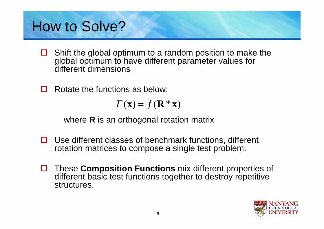
How to Solve?Shift the global optimum to a random position to make the global optimum to have different parameter values for different dimensions
Rotate the functions as below:
where R is an orthogonal rotation matrix
Use different classes of benchmark functions, different rotation matrices to compose a single test problem.
These Composition Functions mix different properties of different basic test functions together to destroy repetitive structures.
( ) ( * )F f=x R x

-7-
Novel Composition Test Functions
Compose the standard benchmark functions to construct a more challenging function with a randomly located global optimum and several randomly located deep local optima with different linkage properties over the search space.
Gaussian functions are used to combine these benchmark functions and to blur individual functions’ structures mainly around the transition regions.
More details in Liang, et al 2005, CEC 2005 special sessions on benchmarking RP-EAs.

-8-
Novel Composition Test Functions
is.

-9-
Novel Composition Test Functions

-10-
Novel Composition Test Functions
define
These composition functions can also be used as multimodal functions.

-11-
A couple of Examples
Many composition functions are available from our homepage
Composition Function 1 (F1):Made of Sphere Functions
Composition Function 2 (F2):Made of Griewank’s Functions
Similar analysis is needed for other benchmarks such as the multi-objective, constrained, etc.

-12-
II - Particle Swarm Optimizer
Introduced by Kennedy and Eberhart in 1995(Eberhart & Kennedy,1995; Kennedy & Eberhart,1995)Emulates flocking behavior of birds, animals, insects, fish, etc. to solve optimization problems Each solution in the landscape is a particleAll particles have fitness values and velocitiesThe standard PSO does not have mutation, crossover, selection ,etc.

-13-
Particle Swarm OptimizerTwo versions of PSO
Global version (May not be used alone to solve multimodal problems): Learning from the personal best (pbest) and the best position achieved by the whole population (gbest)
Local Version: Learning from the pbest and the best position achieved in the particle's neighborhood population (lbest)
The random numbers (rand1 & rand2) should be generated for each dimension of each particle in every iteration.
1 2* 1 ( ) * 2 ( )← ∗ − + ∗ −
← +
d d d d d d di i i i i i
d d di i i
V c rand pbest X c rand gbest X
X X V
1 2* 1 ( ) * 2 ( )← ∗ − + ∗ −
← +
d d d d d d di i i i i k i
d d di i i
V c rand pbest X c rand lbest X
X X V
i – particle counter & d – dimension counter
lbest to be defined w. r. t. a neighborhood.

-14-
General parameters in PSO
and denote the acceleration constants usually set to ~2.and are two uniform random numbers within the
range [0,1]represents the position of the ith particle represents the position changing rate
(velocity) of the ith particlerepresents the best
previous position (the position giving the best objective function value) of the ith particle
represents the best previous position of the whole swarm
represents the best previous position achieved by those particles within the neighborhood of the ith particle
1c 2c
1 2( , ,..., )Di i i ix x x=x
1 2( , ,..., )Di i i ipbest pbest pbest=pbest
1 2( , ,..., )Dgbest gbest gbest=gbest
1 2( , ,..., )Di i i iv v v=v
1 2( , ,..., )Di i i ilbest lbest lbest=lbest
dirand1 d
irand2
-15-
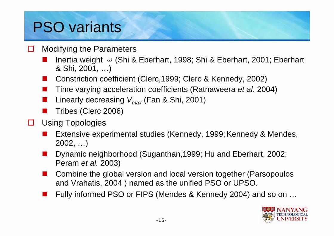
PSO variantsModifying the Parameters
Inertia weight ω (Shi & Eberhart, 1998; Shi & Eberhart, 2001; Eberhart& Shi, 2001, …)Constriction coefficient (Clerc,1999; Clerc & Kennedy, 2002)Time varying acceleration coefficients (Ratnaweera et al. 2004)Linearly decreasing Vmax (Fan & Shi, 2001)Tribes (Clerc 2006)
Using Topologies Extensive experimental studies (Kennedy, 1999; Kennedy & Mendes, 2002, …)Dynamic neighborhood (Suganthan,1999; Hu and Eberhart, 2002; Peram et al. 2003)Combine the global version and local version together (Parsopoulos and Vrahatis, 2004 ) named as the unified PSO or UPSO.Fully informed PSO or FIPS (Mendes & Kennedy 2004) and so on …

-16-
PSO variants and ApplicationsHybrid PSO Algorithms
PSO + selection operator (Angeline,1998)PSO + crossover operator (Lovbjerg, 2001)PSO + mutation operator (Lovbjerg & Krink, 2002; Blackwell & Bentley,2002; … …)PSO + dimension-wise search (Bergh & Engelbrecht, 2004)…
Various Optimization Scenarios & Applications Binary Optimization (Kennedy & Eberhart, 1997; Agrafiotis et. al 2002; )Constrained Optimization (Parsopoulos et al. 2002; Hu & Eberhart, 2002; … )Multi-objective Optimization (Ray et. al 2002; Coello et al. 2002/04; … )Dynamic Tracking (Eberhart & Shi 2001; … )Yagi-Uda antenna (Baskar et al 2005b), Photonic FBG design (Baskar et al 2005a), FBG sensor network design (Liang et al June 2006)

-17-
PSO with Momentum / Constriction
In PSO with momentum [SE98], a momentum term ω is introduced to the original equation:
PSO with constriction factor [CK02]:
di
di
di
di
ddi
di
di
di
di
di
vxx
xgbestrandcxpbestrandcvv
+←
−+−+← )(2)(1 21ω
0.7298. set to be can factor onConstricti
)](2)(1[ 21
χ
χdi
di
di
di
ddi
di
di
di
di
di
vxx
xgbestrandcxpbestrandcvv
+←
−+−+←
ω is usually reduced form 0.9 to 0.4

-18-
PSO Variants by Kennedy et. al
In fully informed particle swarm (FIPS) [KM06, MKN04], each particle’s velocity is adjusted based on contributions from pbest of all its neighbors.
Bare bones PSO [K03]: PSO without the velocity term, i.e. with the social & cognitive terms only.
Essential Particle swarm [K06]: The velocity is expressed as direction defined by the particle’s position at time t and time (t-1), i.e. the persistence and social influence.
Essential Particle Swarm is another realization of the FIPS.
-19-
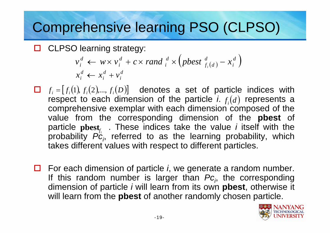
Comprehensive learning PSO (CLPSO)CLPSO learning strategy:
denotes a set of particle indices with respect to each dimension of the particle i. represents a comprehensive exemplar with each dimension composed of the value from the corresponding dimension of the pbest of particle . These indices take the value i itself with theprobability Pci, referred to as the learning probability, which takes different values with respect to different particles.
For each dimension of particle i, we generate a random number. If this random number is larger than Pci, the corresponding dimension of particle i will learn from its own pbest, otherwise it will learn from the pbest of another randomly chosen particle.
( ) ( ) ( )[ ]Dffff iiii ,...,2 ,1=
ifpbest
( )dfi
di
di
di vxx +←
( )( )di
ddf
di
di
di xpbestrandcvwv
i−××+×←

-20-
Tournament selection with size 2 is used to choose the index .
To ensure that a particle learns from good exemplars and to minimize the time wasted on poor directions, we allow each particle to learn from the exemplars until such particle stop toimprove for a certain number of generations, called the refreshing gap m (7 generations). After that, we re - assign for each particle i.
The detailed description and algorithmic implementation can be found in [[LQSB06LQSB06]]. Matlab codes including CLPSO and several state-of-the-art PSO variants are available for academic use.
CLPSO
( )dfi
( ) ( ) ( )[ ]Dffff iiii ,...,2 ,1=
-21-
CLPSOThree major differences between CLPSO and the conventional PSO are highlighted:
Instead of using particle’s pbest and gbest as the exemplars, all particles’ pbests can be used to guide a particle’s flying direction.
Instead of learning from the same exemplar for all dimensions, different dimensions of a particle may learn from different exemplarswithin certain generations. In other words, at one iteration, each dimension of a particle may learn from the corresponding dimension of different particle’s pbest.Instead of learning from two exemplars (pbest and gbest) in every generation, each dimension of a particle in CLPSO learns from just one comprehensive exemplar within certain generations.
Experimental results [[LQSB06LQSB06] ] over a suite of 16 numerical test functions have demonstrated the promising performance of the CLPSO to solve the multi-modal optimization problems in comparison with 8 state-of-the-art PSO variants.

-22-
CLPSO with Probability AdaptationAdaptive Self-Learning Strategy
Assume Pc normally distributed in a range with mean(Pc) and a standard deviation of 0.1. Initially, mean(Pc) is set at 0.5 and different Pc values conforming to this normal distribution are generated for each individual in the current population. During every generation, the Pc values associated with the particles which find new pbest are recorded. The mean of normal distribution of Pc is recalculated according to all the recorded Pc values corresponding to successful movements during the last several generations. As a result, the proper Pc value range for the current problem can be learned to suit the particular problem.

-23-
Dynamic multi-swarm PSO (DMS-PSO)
The population is divided into several sub-swarms randomly.Each sub-swarm utilizes its own particles to search for better solutions and converge to some suboptimal solution.The whole population is re-grouped into new sub-swarms periodically. New sub-swarms continue the search procedure.This process continues until a termination criterion is satisfied.
Regroup
DMS-PSO is constructed based on the local version of PSO with a novel neighborhood topologyTwo major characteristics of the novel neighborhood topology:
Small sized swarms Randomized re-grouping scheme

-24-
DMS-PSO learning strategyEach particle i has an associated vector Pci. After every Rgenerations, an indicator vector keepidi will be updated according to Pci: if randid is larger than or equal to Pci(d), keepidi(d) is set to 1 and the dth dimension of particle i will be set as the value of its own pbesti(d), otherwise keepidi(d) is set to 0, and the dth dimension of particle i will learn from its lbesti(d), and its own pbesti(d), as the PSO with constriction coefficients:
m a x m a x
If _ 0
0 .7 2 9 1 .4 9 4 4 5 1 ( )
1 .4 9 4 4 5 2 ( )
m in ( , m a x ( , ) )
O th e rw is e
di
d d d d di i i i i
d d di i i
d d d di i
d d di i i
d di i
k e e p id
v v r a n d p b e s t x
r a n d lb e s t x
v v v v
x x v
x p b e s t
=
← × + × × −
+ × × −
= −
← +
←
DMS-PSO
Somewhat similar to DE & CPSO

-25-
DMS-PSOParameter adaptation scheme
Assume Pci is normally distributed with mean mean_Pc and standard deviation 0.1. Initially, mean_Pc is set to 0.5 and a set of Pci vectors with respect to each particle i in the current population are generated according to such normal distribution.At each generation, the Pci values associated with those particles that find new pbests are recorded. When sub-swarms are regrouped, mean_Pc is re-calculated according to all the recorded successful Pcivalues. The recorded successful Pci values will be cleared when mean_Pc is recalculated.As a result, a proper Pci distribution with respect to the given problem can be evolved.

-26-
DMS-PSO with local searchAlthough we can achieve larger diversity using DMS-PSO, the convergence rate may slow down. In order to alleviate this problem, a local search procedure is incorporated:
Every L generations, pbests of five randomly chosen particles will be used as the starting points and the Quasi-Newton method is applied to conduct the local search with maximum function evaluations L_FEs.
At the end of the DMS-PSO search, particles in each sub-swarm are grouped into a whole swarm to perform the global PSO. The best solution achieved so far is refined using the Quasi-Newton method every L generations with the 5×L_FEs as the maximum search step.
If local search results in improvements, the nearest pbestis replaced.

-27-
III - Outline of Presentation on DE
Motivation for Differential Evolution (DE)
Classical DE
DE Variants
Self-adaptive DE (SaDE)

-28-
Motivation for DEDE, proposed by Price and Storn in 1995 [PS95], was motivated by the attempts
to use Genetic Annealing [P94] to solve the Chebychev polynomial fitting problem.
Genetic annealing is a population-based, combinatorial optimization algorithm that implements a thermodynamic annealing criterion via thresholds. Although successfully applied to solve many combinatorial tasks, genetic annealing could not solve the Chebychev problem satisfactorily.
Price modified genetic annealing by using floating-point encoding instead of bit-string one, arithmetic operations instead of logical ones, population-driven differential mutation instead of bit-inversion mutation and removed the annealing criterion. Storn suggested creating separate parent and children populations. Eventually, Chebychev problem can be solved effectively.
DE is closely related to many other multi-point derivative free search methods [PSL05] such as evolutionary strategies, genetic algorithms, Nelder and Mead direct search and controlled random search.

-29-
DE at a glanceCharacteristics
Population-based stochastic direct searchSelf-referential mutationSimple but powerfulReliable, robust and efficientEasy parallelizationFloating-point encoding
Basic componentsInitializationTrial vector generation
MutationRecombination
Replacement

-30-
InitializationA population Px,0 of Np D-dimensional parameter vectors xi,0=[x1,i,0,…,xD,i,0], i=1,…,Np is randomly generated within the prescribed lower and upper bound bL= [b1,L,…,bD,L] and bU=[b1,U,…,bD,U]
Insight into classical DE (DE/rand/1/bin)
Trial vector generation
Example: the initial value (at generation g=0) of the jth parameter of the ith vector is generated by: xj,i,0 = randj[0,1] ·(bj,U-bj,L) + bj,L, j=1,…,D, i=1,…,Np
At the At the ggthth generation, a trial population generation, a trial population PPuu,,gg consisting of consisting of NpNp DD--dimensional trial dimensional trial vectors vectors vvi,gi,g=[=[vv1,1,i,gi,g,,……vvDD,,i,gi,g] is generated via mutation and recombination operations ] is generated via mutation and recombination operations applied to the current population applied to the current population PPxx,,gg
Differential mutation: with respect to each vector xi,g in the current population, called target vector, a mutant vector vi,g is generated by adding a scaled, randomly sampled, vector difference to a basis vector randomly selected from the current population
-31-
Insight into classical DE (DE/rand/1/bin)
Replacement
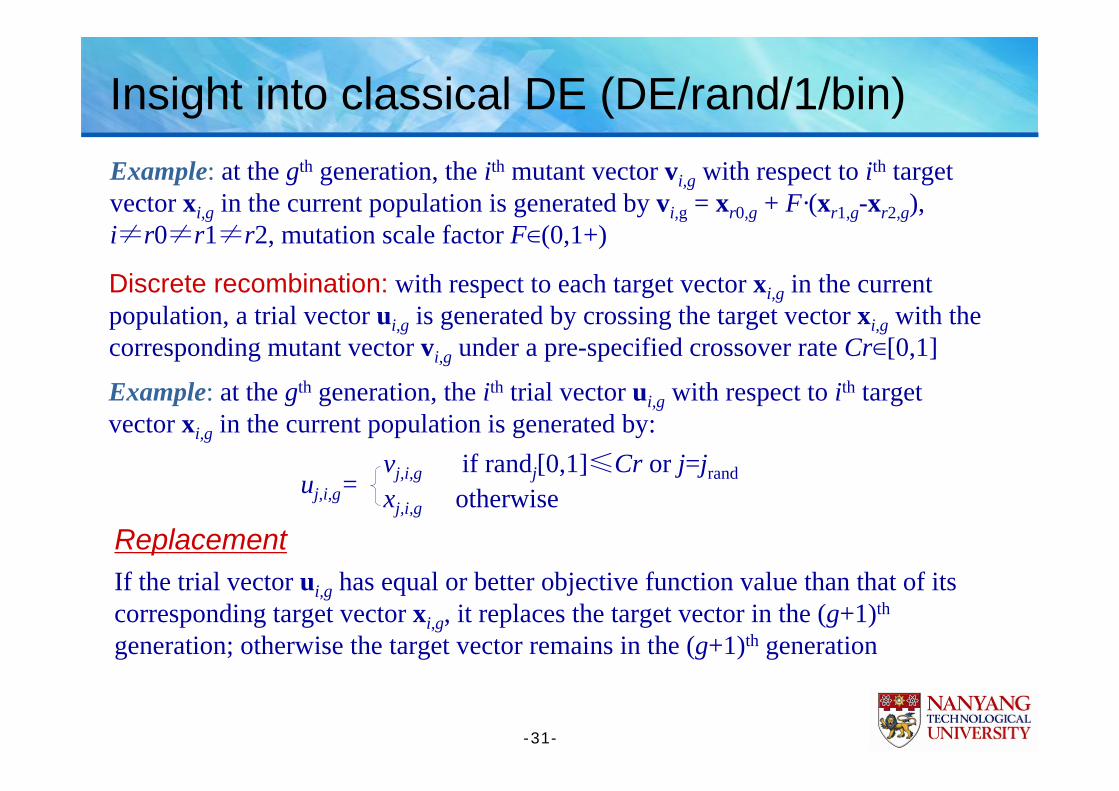
Example: at the gth generation, the ith mutant vector vi,g with respect to ith target vector xi,g in the current population is generated by vi,g = xr0,g + F·(xr1,g-xr2,g), i≠r0≠r1≠r2, mutation scale factor F∈(0,1+)
Discrete recombination: with respect to each target vector xi,g in the current population, a trial vector ui,g is generated by crossing the target vector xi,g with the corresponding mutant vector vi,g under a pre-specified crossover rate Cr∈[0,1]
Example: at the gth generation, the ith trial vector ui,g with respect to ith target vector xi,g in the current population is generated by:
vj,i,g if randj[0,1]≤Cr or j=jrand
xj,i,g otherwiseuj,i,g=
If the trial vector ui,g has equal or better objective function value than that of its corresponding target vector xi,g, it replaces the target vector in the (g+1)th
generation; otherwise the target vector remains in the (g+1)th generation

-32-
Illustration of classical DE
x2
x1
Illustration of classic DE

-33-
xi,g
xr1,g
xr2,g
xr0,g
x2
x1
Target vector
Base vector Two randomly selected vectors
Illustration of classic DE
Illustration of classical DE

-34-
xi,g
xr1,g
xr2,g
xr0,g
x2
x1
Four operating vectors in 2D continuous space
Illustration of classical DE

-35-
xi,g
xr1,g
xr2,g
xr0,g
F·(xr1,g-xr2,g)
vi,g
x2
x1
Trial vector after Mutation
Illustration of classical DE

-36-
xi,g
xr1,g
xr2,g
xr0,g
F·(xr1,g-xr2,g)
vi,g ui,g
x2
x1
Trial vector after Crossover
Illustration of classical DE

-37-
Replacement of target vector by the trial vector
xi,g
xr1,g
xr2,g
xr0,g
xi,g+1
x2
x1
Illustration of classical DE

-38-
Differential vector distribution
Most important characteristics of DE: self-referential mutation!
ES: fixed probability distribution function with adaptive step-size
DE: adaptive distribution of difference vectors with fixed step-size
A population of 5 vectors 20 generated difference vectors

-39-
DE variantsModification of different components of DE can result in many DEModification of different components of DE can result in many DEvariantsvariants:
InitializationUniform distribution and Gaussian distribution
Trial vector generationChoices in base vector selection
Random selection without replacement: r0=ceil(randi[0,1]·Np)
Permutation selection: r0=permute[i]
Random offset selection: r0=(i+rg)%Np (e.g. rg=2)
Biased selection: global best, local best or tournament

-40-
DE variantsDifferential mutation
One difference vector: F·(xr1- xr2) Two difference vector: F·(xr1- xr2)+F·(xr3- xr4)Mutation scale factor F
Crucial role: balance exploration and exploitationDimension dependence?: jitter, if yes (rotation variant) and
dither, if no (rotation invariant).Randomization: different distributions of F
DE/rand/1:DE/best/1:DE/current-to-best/1:DE/rand/2:DE/best/2:
( )GrGrGrGi F ,,,, 321XXXV −⋅+=
( )GrGrGbestGi F ,,,, 21XXXV −⋅+=
( ) ( )GrGrGiGbestGiGi FF ,,,,,, 21XXXXXV −⋅+−⋅+=
( )GrGrGrGrGrGi F ,,,,,, 54321XXXXXV −+−⋅+=
( )GrGrGrGrGbestGi F ,,,,,, 4321XXXXXV −+−⋅+=
-41-
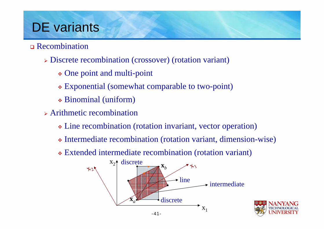
DE variantsRecombination
Discrete recombination (crossover) (rotation variant)One point and multi-pointExponential (somewhat comparable to two-point)Binominal (uniform)
Arithmetic recombinationLine recombination (rotation invariant, vector operation)Intermediate recombination (rotation variant, dimension-wise)Extended intermediate recombination (rotation variant)
x1
x2 xb
xa
line
discrete
discrete
intermediate
x 1x 2

-42-
Motivation for self-adaptation in DEThe performance of DE on different problems depends on:
Population sizeStrategy and the associated parameter setting to generate trial vectorsReplacement scheme
It is hard to choose a unique combination to successfully solve any problem at hand
Population size usually depends on the problem scale and complexityDuring evolution, different strategies coupled with specific parameter settingsmay be effective for different search stages.Replacement schemes influence the population diversityTrial and error scheme may be a waste of computational time & resources
Automatically adapt the configuration in DE so as to generate efAutomatically adapt the configuration in DE so as to generate effective fective trial vectors during evolutiontrial vectors during evolution

-43-
Related worksPractical guideline [SP95], [SP97], [CDG99], [BO04], [PSL05],[GMK02]: for example, Np∈[5D,10D]; Initial choice of F=0.5 and CR=0.1/0.9; Increase NP and/or Fif premature convergence happens. Conflicting conclusions with respect to different Conflicting conclusions with respect to different test functions.test functions.
Fuzzy adaptive DE [LL02]: use fuzzy logical controllers whose inputs incorporate the relative function values and individuals of successive generations to adapt the mutation and crossover parameters.
Self-adaptive Pareto DE [A02]: encode crossover rate in each individual, which is simultaneously evolved with other parameters. Mutation scale factor is generated for each variable according to Gaussian distribution N(0,1).
Zaharie [Z02]: theoretically study the DE behavior so as to adapt the control parameters of DE according to the evolution of population diversity.
Self-adaptive DE (1) [OSE05]: encode mutation scale factor in each individual, which is simultaneously evolved with other parameters. Crossover rate is generated for each variable according to Gaussian distribution N(0.5,0.15).
DE with self-adaptive population [T06]: population size, mutation scale factor and crossover rate are all encoded into each individual.

-44-
Self-Adapting Control Parameters in DE
[BGBMZ06] jDE algorithm encodes mutation scale factor F and crossover rate CR in each individual.
New values for F & CR are assigned to each individual from a set of values and the assignment is performed randomly with respect to pre-specified 2 parameter values.
jDE2 algorithm [BBG06] introduces re-initialization of poorly performing individuals to the jDE algorithm.

-45-
Steps:1. Initialize selection probability pi=1/num_st, i=1,…,num_st for each strategy2. According to the current probabilities, we employ stochastic universal
selection to assign one strategy to each target vector in the current population 3. For each strategy, define vectors nsi and nfi, i=1,…num_st to store the number
of trial vectors successfully entering the next generation or discarded by applying such strategy, respectively, within a specified number of generations, called “learning period (LP)”
4. Once the current number of generations is over LP, the first element of nsi and nfi with respect to the earliest generation will be removed and the behavior in current generation will update nsi and nfi
Self-adaptive DE (SaDE)
Strategy adaptation: select one strategy from a pool of candidate strategies with the probability proportional to its previous successful rate to generate effective trial vectors during a certain learning period
DE with strategy and parameter self-adaptation [QS05, HQS06]

-46-
Self-adaptive DE (SaDE)
Parameter adaptationMutation scale factor (F): for each target vector in the current population, we randomly generate F value according to a normal distribution N(0.5,0.3). Therefore, 99% F values fall within the range of [–0.4,1.4]
Crossover rate (CRj): when applying strategy j with respect to a target vector, the corresponding CRj value is generated according to an assumed distribution, and those CRj values that have generated trial vectors successfully entering the next generation are recorded and updated every LP generations so as to update the parameters of the CRj distribution. We hereby assume that each CRj, j=1,…,num_st is normally distributed with its mean and standard deviation initialized to 0.5 and 0.1, respectively
5. The selection probability pi is updated by:
nsnum_st(L)…ns1(L)
…
nsnum_st(1)…ns1(1)
nsnum_st(L+1)…ns1(L+1)
…
nsnum_st(2)…ns1(2)
nsnum_st(L+2)…ns1(L+2)
…nsnum_st(3)…ns1(3)
…
( )∑+∑∑ iii nfnsns . Go to 2nd step

-47-
Instantiations
In CEC’05, we use 2 strategies:
In CEC’06, we employ 4 strategies:
( )GrGrGrGi F ,,,, 321XXXV −⋅+=
DE/rand/1/bin:
DE/rand/2/bin:
DE/current-to-best/2/bin:
DE/current-to-rand/1:
( )GrGrGrGi F,321 ,,, XXXV −⋅+=
( ) ( )GrGrGrGrGiGbestGiGi FF ,,,,,,,, 4321XXXXXXXV −+−⋅+−⋅+=
( )GrGrGrGrGrGi F,54,321 ,,,, XXXXXV −+−⋅+=
DE/rand/1/bin:
DE/current-to-best/2/bin: ( ) ( )GrGrGrGrGiGbestGiGi FF ,,,,,,,, 4321XXXXXXXV −+−⋅+−⋅+=
( ) ( )GrGrGiGrGiGi FF ,,,,,, 321XXXXXV −⋅+−⋅+=
LP = 50
LP = 50

-48-
Local search enhancement
To improve convergence speed,To improve convergence speed, we apply a local search we apply a local search procedure every 500 generations:procedure every 500 generations:
To apply local search, we choose n = 0.05·Np individuals, which include the individual having the best objective function value and the n-1 individuals randomly selected from the top 50% individuals in the current population
We perform the local search by applying the Quasi-Newton method to the selected n individuals

-49-
Overview of DE research trends
Digital Filter Design
Multiprocessor synthesis
Neural network learning
Diffraction grating design
Crystallographic characterization
Beam weight optimization in radiotherapy
Heat transfer parameter estimation in a trickle bed reactor
Electricity market simulation
Scenario-Integrated Optimization of Dynamic Systems
Optimal Design of Shell-and-Tube Heat Exchangers
Optimization of an Alkylation's Reaction
Optimization of Thermal Cracker Operation
Optimization of Non-Linear Chemical Processes
Optimum planning of cropping patterns
Optimization of Water Pumping System
Optimal Design of Gas Transmission Network
Differential Evolution for Multi-Objective Optimization
Bioinformatics
DE Applications

-50-
IV - Constrained Optimization
Optimization of constrained problems is an important area in the optimization field. In general, the constrained problems can be transformed into the following form:
Minimize subjected to:
q is the number of inequality constraints and m-q is the number of equality constraints.
1 2( ), [ , ,..., ]Df x x x=x x
( ) 0, 1,...,jh j q m= = +x
( ) 0, 1,...,ig i q≤ =x

-51-
Constrained OptimizationFor convenience, the equality constraints can be transformed into inequality form:
where is the allowed tolerance.
Then, the constrained problems can be expressed asMinimize
subjected to
If we denote with the feasible region and the whole search space, if and all constraints are satisfied. In this case,x is a feasible solution.
| ( ) | 0jh ε− ≤x
ε
F∈x S∈xF S
1 2( ), [ , ,..., ]Df x x x=x x
1,..., 1,... 1,..., 1,...
( ) 0, 1,..., ,
( ) ( ), ( ) ( ) ε+ +
≤ =
= = −
j
q q q m q m
G j m
G g G h
x
x x x x

-52-
Constraint-Handling (CH) Techniques
Penalty Functions: Static Penalties (Homaifar et al.,1994;…)Dynamic Penalty (Joines & Houck,1994; Michalewicz& Attia,1994;…)Adaptive Penalty (Eiben et al. 1998; Coello, 1999; Tessema & Gary Yen 2006, Smith & Tate 1993…)…
Superiority of feasible solutionsStart with a population of feasible individuals (Michalewicz, 1992; Hu & Eberhart, 2002; …)Feasible favored comparing criterion (Ray, 2002; Takahama & Sakai, 2005; … )Specially designed operators (Michalewicz, 1992; …)…

-53-
Constraint-Handling (CH) Techniques
Separation of objective and constraintsStochastic Ranking (Runarsson & Yao, TEC, Sept 2000)Co-evolution methods (Coello, 2000a)Multi-objective optimization techniques (Coello, 2000b; Mezura-Montes & Coello, 2002;… )Feasible solution search followed by optimization of objective (Venkatraman & Gary Yen, 2005)…
While most CH techniques are modular (i.e. we can pick one CH technique and one search method independently), there are also CH techniques embedded as an integral part of the EA.

-54-
DMS-PSO for Constrained Optimization
Novel Constraint-Handling MechanismSuppose that there are m constraints, the population is divided into n sub-swarms with sn members in each sub-swarm and the population size is ps (ps=n*sn). n is a positive integer and ‘n=m’ is not required.
The objective and constraints are assigned to the sub-swarms adaptively according to the difficulties of the constraints.
By this way, it is expected to have population of feasible individuals with high fitness values.

-55-
DMS-PSO’s Constraint-Handling Mechanism
How to assign the objective and constraints to each sub-swarm?
Define
Thus 1 21 , [ , ,..., ]mfp p p p= − =p p
10
if a ba b
if a b>⎧
> = ⎨ ≤⎩
1
( ( ) 0), 1, 2,...,
ps
i jj
i
gp i m
ps=
>= =∑ x
1( / ) 1
m
ii
fp p m=
+ =∑
p

-56-
DMS-PSO’s Constraint-Handling Mechanism
For each sub-swarm,Using roulette selection according to fp and to assign the objective function or a single constraint as its target. If sub-swarm i is assigned to improve constraint j, set obj(i)=j and if sub-swarm i is assigned to improve the objective function, set obj(i)=0.
Assigning swarm member for this sub-swarm: Sort the unassigned particles according to obj(i), and assign the best and sn-1 worst particles to sub-swarm i.
/ip m

-57-
DMS-PSO’s Comparison Criteria
1. If obj(i) = obj(j) = k (particle i and j handling the same constraint k), particle i wins if
2. If obj(i) = obj(j) = 0 (particle i and j handling f(x) ) or obj(i) ≠ obj(j) (iand j handling different objectives), particle i wins if
( ) ( ) with ( ) 0
( ) ( ) & ( ), ( ) 0
( ) ( ) & ( ) ( )
< >
< ≤
< ==
k i k j k j
i j k i k j
i j i j
G G G
or V V G G
or f f V V
x x x
x x x x
x x x x
( ) ( )
( ) ( ) & ( ) ( )
<
< ==i j
i j i j
V V
or f f V V
x x
x x x x
1( ) ( ( ) ( ( ) 0))
=
= ⋅ ⋅ ≥∑m
i i ii
V weight G Gx x x
1
1/ max, 1, 2,...
(1/ max)=
= =
∑i
i m
ii
Gweight i m
G

-58-
DMS-PSO for Constrained Optimization
Step 1: Initialization -Initialize ps particles (position X and velocity V), calculate f(X), Gj(X) (j=1,2...,m) for each particle.
Step 2: Divide the population into sub-swarms and assign obj for each sub-swarm using the novel constraint-handling mechanism, calculate the mean value of Pc (except in the first generation, mean(Pc)=0.5), calculate Pc for each particle. Then empty Pc.
Step 3: Update the particles according to their objectives; update pbest and gbest of each particle according to the same comparison criteria, record the Pc value if pbest is updated.

-59-
Step 5: Local Search-Every L generations, randomly choose 5 particles’ pbest and start local search with Sequential Quadratic Programming (SQP) method using these solutions as start points (fmincon(…,…,…) function in Matlab is employed). The maximum fitness evaluations for each local search is L_FEs.
Step 6: If FEs≤0.7*Max_FEs, go to Step 3. Otherwise go to Step 7.
Step 7: Merge the sub-swarms into one swarm and continue PSO (Global Single Swarm). Every L generations, start local search using gbest as start points using 5*L_FEs as the Max FEs. Stop search if FEs≥Max_FEs
DMS-PSO for Constrained Optimization

-60-
SaDE for Constrained Optimization
Strategy AdaptationProbabilistically select one out of several available learning strategies to apply for each individual in the current population
DE/Rand/1:
DE/Current to best/2:
DE/Rand/2:
DE/Current-to-rand/1:
( )GrGrGrGi F,321 ,,, XXXV −⋅+=
( ) ( )GrGrGrGrGiGbestGiGi FF,43,21 ,,,,,, XXXXXXXV −+−⋅+−⋅+=
( ) ( )GrGrGrGrGrGi FF,54,321 ,,,, XXXXXV −⋅+−⋅+=
( ) ( )1 3 1 2,, , , , ,i G r G r G i G r G r GU K F= + ⋅ − + ⋅ −X X X X X

-61-
Self-adaptive Differential Evolution
Initial probabilities p1=p2=p3=p4=0.25
According to the probability, we apply Stochastic Universal Selection to select the strategy for each individual in the current population.
nsi (nfi), i=1,2,3,4: the accumulated number of trial vectors, successfully entering (discarded) the next generation while generated by each strategy
nsi and nfi are accumulated within a specified number of generations, called the “learning period (LP)”. The probability pi is updated as:
nfnsnspi
ii +=

-62-
Self-adaptive Differential Evolution
F: different random values normrnd(0.5,0.3) in the range (0,2] for different individuals
CR: accumulating the previous learning experience within a certain generational interval so as to dynamically adapt the value of CR
to a suitable range
Parameters adaptation
IF REM (G, LP)=0 CRm=mean(CRpool)
END IF
IF REM (G, 5)=0FOR i =1 to NP
CRi=normrand(CRm,0.1)END FOR
END IF

-63-
Extend SaDE to Handle Constraints
Selection procedureThe trial vector Ui,G is compared to its corresponding target vector Xi,G in the current population considering both the fitness value and constraints.
Ui,G will replace Xi,G if any of the following conditions is true1. Ui,G is feasible, Xi,G is not.2. Ui,G and Xi,G are both feasible, and Ui,G has smaller or
equal fitness value (for minimization problem) than Xi,G .3. Ui,G and Xi,G are both infeasible, but Ui,G has a smaller
overall constrain violation.

-64-
Local Search
To speed up the convergence, we apply a local search procedure once every 500 generations
n=5% of NP individuals
DE_gbest + randomly selected n-1 individuals from the best 50% individuals in the current population
We employ the Sequential Quadratic Programming (SQP) method as the local search method.

-65-
V - Multi-objective Problems [D01]Many real-world problems involve multiple, conflicting objectives
Applications: [CVL02][CVL02], [SP05][SP05], [MB06][MB06], [TLL05][TLL05]
Robotics and control engineeringTransport engineeringSchedulingFinanceBioinformatics Pattern recognitionPID designNon-dominated solutions: In a set of
solutions P, the non-dominated set of solutions P′ are those that are not dominated by any member of the set P .
Pareto-optimality: When the set P is the entire search space, the resulting P′is called the Pareto-optimal set.

-66-
Multi-Objective Optimization
Mathematically, we can use the following formula to express the multi-objective optimization problems (MOP):
The objective of multi-objective optimization is to find a set of solutions which can represent the Pareto-optimal set well, thus there are two goals for the optimization:
1) Convergence to the Pareto-optimal set 2) Diversity of solutions in the Pareto-optimal set
1 2Minimize ( ) ( ( ), ( ), , ( )) [ , ]subject to ( ) 0, 1,...,
( ) 0, 1,...,
m
j
k
f f f fg j z
h k q m
= = ∈≤ =
= = +
y x x x x x Xmin Xmaxx
x
K

-67-
Representative MOEAs [CJKO01][CJKO01][D01][D01][ZLT01][ZLT01][CVL02][AJG05][TKL05][CVL02][AJG05][TKL05]
Non-elitist MOEAsWeight based GA (WBGA)
Multiple objective GA (MOGA)
Niched Pareto GA
Non-dominated sorting GA(NSGA)
Elitist MOEAsDistance-based Pareto GA (DPGA)
Strength Pareto GA (SPEA), SPEA-II
Non-dominated GA-II (NSGA-II)
Pareto-archived ES (PAES),
Pareto envelope-based selection algorithm (PESA), PESA-II
Multi-objective messy GA (MOMGA)

-68-
From PSO to MOPSO
Mainly used techniques:External archive for the non-dominated solution set.How to update pbest and gbest (or lbest)
Execute non-domination comparison with pbest or gbestExecute non-domination comparison among all particles’pbests and their offspring in the entire population
How to choose gbest (or lbest)Choose gbest (or lbest) from the recorded non-dominated solutionsChoose good local guides
How to keep diversityCrowding distance sortingSubpopulation

-69-
From CLPSO and DMS-PSO to MOPSOs
Combine an external archive which is used to record the non-dominated solutions found so far.
Use Non-dominated Sorting and Crowding distance Sorting which have been used in NSGAII (Deb et al., 2002) to sort the members in the external archive.
Choose exemplars (CLPSO) or lbest (DMS-PSO) from the non-dominated solutions recorded in the external archive.
Experiments show that MO-CLPSO and DMS-MO-PSO are both capable of converging to the true Pareto optimal front and maintaining a good diversity along the Pareto front.

-70-
Selection of pbest, gbest in MO-CLPSO [HSL06]
Selection of gbest in MOCLPSOall the non-dominated solutions are good individuals
Randomly choose a particle from the non-dominated solutions.
Other alternatives would be to form grids in the objective space and to select representatives from each cells, or to select more from less crowded cells, etc.
Selection of pbest

-71-
MO-CLPSO Algorithm
1) Initialize Randomly initialize particle positions, Initialize particle velocitiesEvaluate the fitness values of particles, initialize the external archive.2) OptimizeWHILE stopping criterion is not satisfied
DOFor i=1 to NPSelect gbest from external archive
Assign each dimension to learn from gbest, pbest of this particle and pbests of other particles,

-72-
MO-CLPSO Algorithm (cont.)
Update particle velocity
Update particle position
Evaluate the fitness values of particleUpdate pbest if current position is better than pbestEnd ForUpdate the external archiveIncrement the generation countEND WHILE
( )
( ) 1( ) ( ) () ( ( ) ( ))( ) 1
( ) ( ) () ( ( ) ( ))
( ) ( ) () ( ( ) ( ))
i
i k i i
i
i k i fi d i
i k i i i
if a dV d V d rand gbest d X d
if b dV d V d rand pbest d X d
elseV d V d rand pbest d X d
ω
ω
ω
==⎧⎪ = ∗ + ∗ −⎪⎪ ==⎪⎨ = ∗ + ∗ −⎪⎪⎪
= ∗ + ∗ −⎪⎩
( ) ( ) ( )i i iX d X d V d= +

-73-
MO-DMS-PSO Algorithm
The solutions in the external archive are sorted based on one randomly chosen objective and then partitioned into n groups where n is the number of sub-swarms.Each sub-swarm randomly selects one representative as the gbest from each partition of the external archive.
-74-
MOSaDE
MOSaDE is an extension of SaDE to optimize problems with multiple objectives. Similar to SaDE, the MOSaDE algorithm automatically adapts the trial vector generation strategies and their associated parameters according to their previous experience of generating promising or inferior individuals. However, when extending the single-objective algorithm to multi-objective domain, the evaluation criteria of promising or inferior individuals must be changed.

-75-
MOSaDE
We use the following: Individual A is better than individual B, if(1) individual A dominates B, or (2) individual A and individual B are non-
dominated with each other, but A is less crowded than individual B. Therefore, in case that the trial vector is better than the target vector according to this criterion, we will record the associated parameter and strategy.

-76-
MOSaDEThe strategies incorporated into our proposed MOSaDEalgorithm are ‘rand/1/bin’ and ‘best/2/bin’. The Xbest in ‘best/2/bin’ is randomly selected from external archive.
MOSaDE AlgorithmStep 1. Randomly initialize a population of NP individuals. Initialize strategy probability (pk, k=1,…,K, K is the no. of available strategies), the median value of CR(CRmk) for each strategy, learning period (LP=50) .Step 2. Evaluate the individuals in the population, and fill the external archive with these individuals.

-77-
MOSaDE Algorithm
Step 3.Repeat(1) Calculate strategy probability pk: the percentage of the success rate of trial
vectors generated by each strategy during the learning period.(2) Assign trial vector generation strategy and parameters to each target vector
Xi
(a) Use stochastic universal sampling to select one strategy k for each target vector Xi
(b) Assign control parameters F and CRF: Generate the F values under Normrnd(0.3,0.1) CR: After the first LP generation, calculate CRmk according to the recorded CR values. Generate the CR values under Normrnd(CRmk,0.1)
(3) Generate a new population where each trial vector is generated according to associated trial vector generation strategy k and parameter F and CR in (2).
(4) Selection:

-78-
FOR i=1:NP(a) Evaluate the trial vector , and compare with the target vector Xn(i)nearest to the trial vector in the solution space.
IF Xn(i) dominates , discard .ELSE
IF dominates Xn(i) ,replace Xn(i) with ;IF non-dominated with each other, choose less crowded one to be
the new target vector; will enter the external archive if (i) dominates some
individual(s) of the archive (the dominated individuals in the archive are deleted); or (ii) is nondominated with archived individuals
END IF(b) If trial vector is better than Xn(i), record the associated parameter CR
and flag strategy k as successful strategy. Otherwise, flag strategy k as failed strategy.
(c) When the external archive exceeds the maximum specified size, we select the less crowded individuals based on harmonic average distance to keep the archive size.
END FOR
kiU
kiU
kiU
kiU
kiU
kiU k
iU
kiU

-79-
Local search
Use local search to further improve solutions found by the MOSaDE algorithm. Employ the Quasi-Newton method as the local search method, considering only one objective randomly selected each time. The local search procedure is applied once every 200 generations, on 10 individuals randomly selected among the non-dominated solutions that were not applied local search previously.

-80-
VI - Niching Methods [SD-06]: Fitness sharing
Fitness sharing [GR-87] modifies the search landscape by reducing the fitness of individuals in densely-populated regions. A sharing radius σs is used to determine whether two individuals share the same niche.Reducing an individual’s fitness is controlled by two operations, a similarity function and a sharing function. The shared fitness fi’ is given by the formula as below:
where fi denotes the original fitness of the individual i, N the population size, and dij the distance between the individual i and the individual j. α is a constant parameter which regulates the shape of the sharing function sh (typically α=1).
The effect of this scheme is to encourage search in unexplored regions. The weakness of this method lies in the fact that it requires a priori knowledge about the distance between the peaks in the search space.

-81-
k-means clustering based
K-means clustering algorithm is used to divide the population into niches [YG-93]. The fitness is calculated based on the distance dic between the individual and its niche centroid.The final fitness of an individual is calculated by the relation:
nc is the number of individuals in the niche containing individual i, dmax is the maximum distance allowed between an individual and its niche centroid, and α is a constant.The formation of the niches is based on the adaptive K-mean algorithm. The algorithm begins with a fixed number (k) of seed points taken as the best k individuals.Using a minimum allowable distance dmin between niche centroids, a few clusters are formed from the seed points.The remaining population members are then added to these existing clusters or are used to form new clusters based on dmin and dmax. These computations are performed in each generation.

-82-
Deterministic crowding (DC)
Deterministic crowding [M-95] is an extension of a technique first used by De Jong to help promote diverse populations [D-75]. After crossover and mutation, the offspring then replace their closest parent if it has a better fitness.Calculate the distances between p1 and c1, p2 and c2, p1 and c2, p2 and c1, and name them d1, d2, d3, d4 respectively.
If d1+d2 <= d3+d4, thenIf the fitness of c1 is higher than the fitness of p1, replace p1 with c1;If the fitness of c2 is higher than the fitness of p2, replace p2 with c2.
ElseIf the fitness of c2 is higher than the fitness of p1, replace p1 with c2;If the fitness of c1 is higher than the fitness of p2, replace p2 with c1.
Deterministic crowding uses a distance measure to determine similarity between individuals. As, DC does not require the use of a similarity radius, this relaxes the requirement of a priori domain knowledge and makes DC more suitable for difficult problems than fitness sharing. DC is an elitist niching method. This means that once a peak is discovered, it is never lost from the population.

-83-
Restricted tournament selection (RTS)
RTS [H-94] adapts tournament selection for multimodal optimization. It initially selects two elements from the population to undergo crossover and mutation. Then a random sample of w individuals is taken from the population to be compared with each offspring created, and the most similar (or the closest) individual is chosen to compete with the offspring. If the offspring wins, it is allowed to enter thepopulation.
-84-
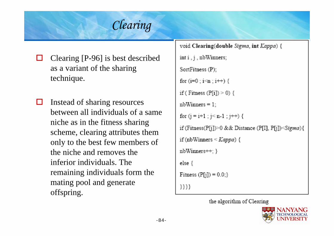
Clearing
Clearing [P-96] is best described as a variant of the sharing technique.
Instead of sharing resources between all individuals of a same niche as in the fitness sharing scheme, clearing attributes them only to the best few members of the niche and removes the inferior individuals. The remaining individuals form the mating pool and generate offspring.

-85-
K-means Clustering-based Niched PSO
Kennedy proposed the nichedPSO using K-means clustering [K-00]. The gbest / pbest / lbest were replaced by cluster centers or the best particle of each cluster to obtain several variants.Clustering-based variants performed better than the original PSO.

-86-
Deflection, Stretching, Repulsion based Niched PSO
Parsopoulos [PV04b] et. al made use of deflection, stretching, repulsion, etc. to locate as many optima as possible.These techniques transform the objective function to make previously obtained local optima to have high function values (or low fitness).

-87-
NichePSO [BEB07]

-88-
VII - BINARY PSO ALGORITHM
Binary PSO (K&E97)Sigmoid function
Force the real values between 0 and 1Velocity is updated with traditional equationSigmoid function is used to squash them to be within [0,1]
s(vij)=1/(1+exp(-vij))Xij=1 if r ≤ s(vij)Xij=0 if r > s(vij)r=uniform random number

-89-
Angle Modulated PSO / DE [PFE05, PEF06]
•a, b, c and d are real valued variables to be optimized by the PSO or DE.
•If there are 10 binary variables, x takes 10 different values, for example, from 1 to 10.
•For every solution of “a, b, c and d” binary bits are generated by sign(g(x)) operation (as x runs from 1 to 10 in the case 10 bit problem.

-90-
VIII - Benchmarking Evolutionary Algorithms
CEC05 comparison results (Single obj. + bound const.)
CEC06 comparison results (Single obj + general const.)
Experimental Results on MOPSOsCEC07 comparison results on MOEAs
CEC benchmarking resources available from http://www.ntu.edu.sg/home/epnsugan/
-91-
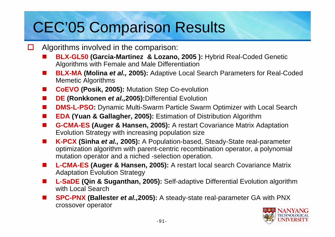
CEC’05 Comparison ResultsAlgorithms involved in the comparison:
BLX-GL50 (Garcia-Martinez & Lozano, 2005 ): Hybrid Real-Coded Genetic Algorithms with Female and Male DifferentiationBLX-MA (Molina et al., 2005): Adaptive Local Search Parameters for Real-Coded Memetic AlgorithmsCoEVO (Posik, 2005): Mutation Step Co-evolutionDE (Ronkkonen et al.,2005):Differential EvolutionDMS-L-PSO: Dynamic Multi-Swarm Particle Swarm Optimizer with Local SearchEDA (Yuan & Gallagher, 2005): Estimation of Distribution AlgorithmG-CMA-ES (Auger & Hansen, 2005): A restart Covariance Matrix Adaptation Evolution Strategy with increasing population sizeK-PCX (Sinha et al., 2005): A Population-based, Steady-State real-parameter optimization algorithm with parent-centric recombination operator, a polynomial mutation operator and a niched -selection operation.L-CMA-ES (Auger & Hansen, 2005): A restart local search Covariance Matrix Adaptation Evolution StrategyL-SaDE (Qin & Suganthan, 2005): Self-adaptive Differential Evolution algorithm with Local SearchSPC-PNX (Ballester et al.,2005): A steady-state real-parameter GA with PNX crossover operator

-92-
CEC’05 Comparison Results
Problems: 25 minimization problems (Suganthan et al. 2005)Dimensions: D=10, 30Runs / problem: 25 Max_FES: 10000*D (Max_FES_10D= 100000; for 30D=300000; for 50D=500000)Initialization: Uniform random initialization within the search space, except for problems 7 and 25, for which initialization ranges are specified. The same initializations are used for the comparison pairs (problems 1, 2, 3 & 4, problems 9 & 10, problems 15, 16 & 17, problems 18, 19 & 20, problems 21, 22 & 23, problems 24 & 25). Global Optimum: All problems, except 7 and 25, have the global optimum within the given bounds and there is no need to perform search outside of the given bounds for these problems. 7 & 25 are exceptions without a search range and with the global optimum outside of the specified initialization ranges.

-93-
CEC’05 Comparison Results
Termination: Terminate before reaching Max_FES if the error in the function value is 10-8 or less.Ter_Err: 10-8 (termination error value)Successful Run: A run during which the algorithm achieves the fixed accuracy level within the Max_FES for the particular dimension.Success Rate= (# of successful runs) / total runsSuccess Performance = mean (FEs for successful runs)*(# of total runs) / (# of successful runs)

-94-
CEC’05 Comparison ResultsSuccess Rates of the 11 algorithms for 10-D
*In the comparison, only the problems in which at least one algorithm succeeded once are considered.

-95-
CEC’05 Comparison Results
Empirical distribution over all successful functions for 10-D (SP here means the Success Performance for each problem. SP=mean (FEs for successful runs)*(# of total runs) / (# of successful runs). SPbest is the minimal FES of all algorithms for each problem.)
First three algorithms:1. G-CMA-ES2. DE3. DMS-L-PSO

-96-
CEC’05 Comparison Results
Success Rates of the 11 algorithms for 30-D
*In the comparison, only the problems which at least one algorithm succeeded once are considered.
-97-
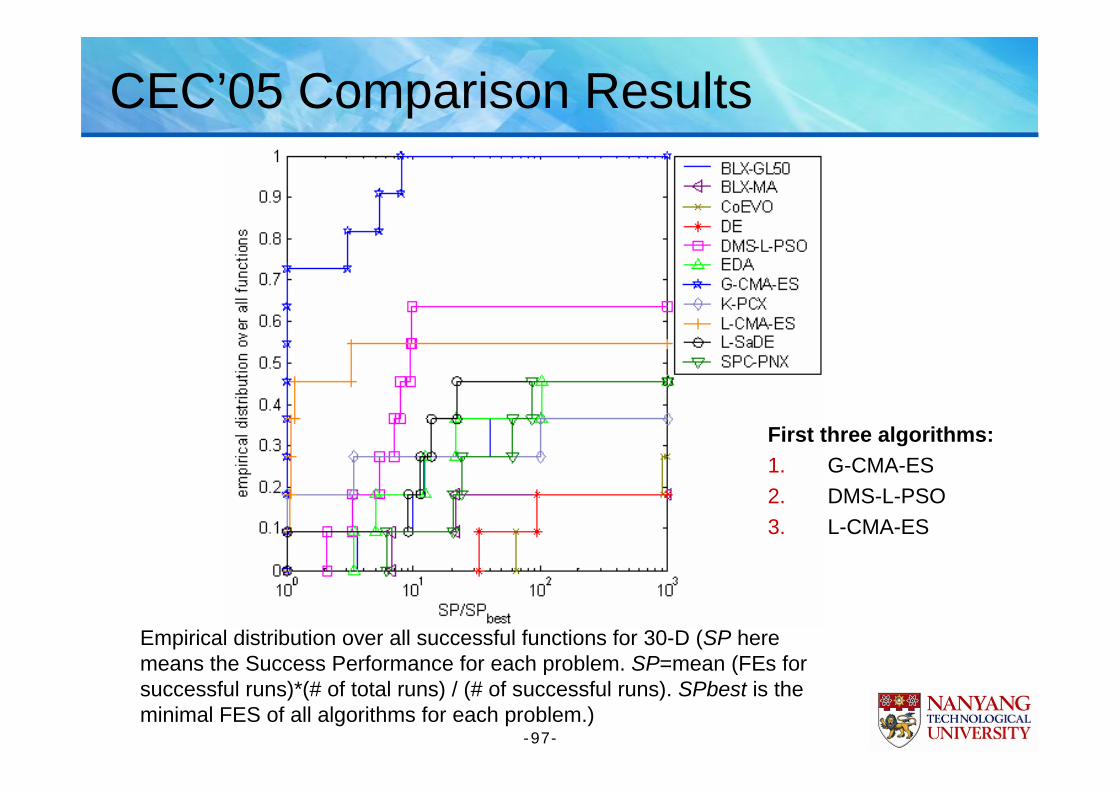
CEC’05 Comparison Results
Empirical distribution over all successful functions for 30-D (SP here means the Success Performance for each problem. SP=mean (FEs for successful runs)*(# of total runs) / (# of successful runs). SPbest is the minimal FES of all algorithms for each problem.)
First three algorithms:1. G-CMA-ES2. DMS-L-PSO3. L-CMA-ES
-98-
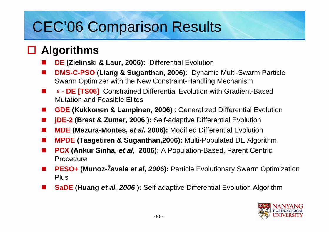
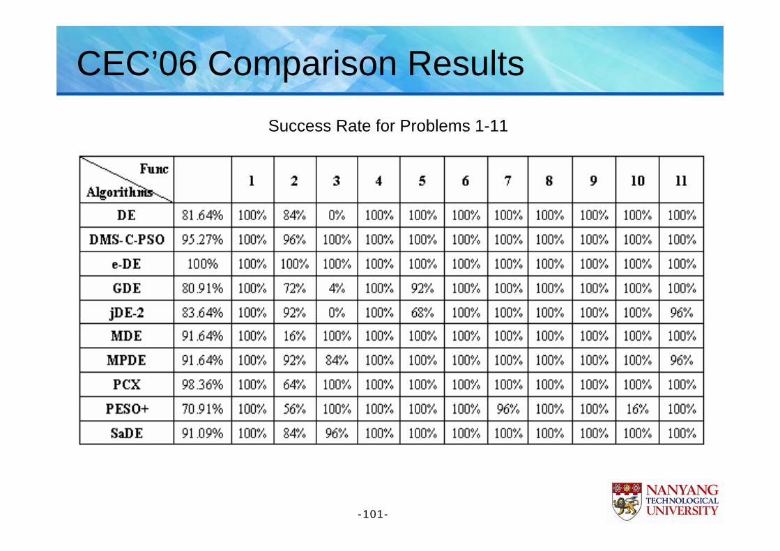
CEC’06 Comparison ResultsAlgorithms
DE (Zielinski & Laur, 2006): Differential Evolution DMS-C-PSO (Liang & Suganthan, 2006): Dynamic Multi-Swarm Particle Swarm Optimizer with the New Constraint-Handling Mechanismε- DE [TS06] Constrained Differential Evolution with Gradient-Based Mutation and Feasible ElitesGDE (Kukkonen & Lampinen, 2006) : Generalized Differential Evolution jDE-2 (Brest & Zumer, 2006 ): Self-adaptive Differential EvolutionMDE (Mezura-Montes, et al. 2006): Modified Differential EvolutionMPDE (Tasgetiren & Suganthan,2006): Multi-Populated DE AlgorithmPCX (Ankur Sinha, et al, 2006): A Population-Based, Parent Centric ProcedurePESO+ (Munoz-Žavala et al, 2006): Particle Evolutionary Swarm Optimization PlusSaDE (Huang et al, 2006 ): Self-adaptive Differential Evolution Algorithm
-99-
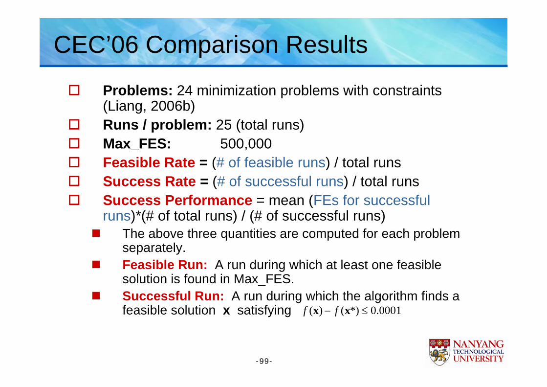
CEC’06 Comparison Results
Problems: 24 minimization problems with constraints (Liang, 2006b)Runs / problem: 25 (total runs)Max_FES: 500,000 Feasible Rate = (# of feasible runs) / total runsSuccess Rate = (# of successful runs) / total runsSuccess Performance = mean (FEs for successful runs)*(# of total runs) / (# of successful runs)
The above three quantities are computed for each problem separately. Feasible Run: A run during which at least one feasible solution is found in Max_FES.Successful Run: A run during which the algorithm finds a feasible solution x satisfying ( ) ( *) 0.0001f f− ≤x x

-100-
CEC’06 Comparison Results
ωNP, LP, LS_gapSaDE
, c1, c2 , n, not sensitive to , c1, c2PESO+N , λ, r (a different N is used for g02), PCXF, CR, np1, np2MPDEμ, CR, Max_Gen, λ, Fα, Fβ,MDENP, F, CR, k, ljDE-2NP, F, CRGDEN, F, CR, Tc, Tmax, cp, Pg, Rg, Neε_DE, c1, c2 , Vmax, n, ns, R, L, L_FESDMS-PSO
NP, F, CRDEω
ω
Algorithms’ Parameters
-101-
CEC’06 Comparison ResultsSuccess Rate for Problems 1-11

-102-
CEC’06 Comparison Results
Success Rate for Problems 12-19,21,23,24

-103-
CEC’06 Comparison Results
Empirical distribution over all functions( SP here means the Success Performancefor each problem. SP=mean (FEs for successful runs)*(# of total runs) / (# of successful runs). SPbest is the minimal FES of all algorithms for each problem.)
GDE, PESO+9th
jDE-28th
DE7th
MPDE6th
SaDE5th
MDE, PCX3rd
DMS-PSO2nd
ε_DE1st

-104-
Results of MOCLPSO on ZDT1
0 0.1 0.2 0.3 0.4 0.5 0.6 0.7 0.8 0.9 10
0.1
0.2
0.3
0.4
0.5
0.6
0.7
0.8
0.9
1
f1
f2
True Pareto FrontMOCLPSO
0 0.1 0.2 0.3 0.4 0.5 0.6 0.7 0.8 0.9 10
0.2
0.4
0.6
0.8
1
1.2
1.4
f1f2
True Pareto FrontMOPSO
0 0.1 0.2 0.3 0.4 0.5 0.6 0.7 0.8 0.9 10
0.2
0.4
0.6
0.8
1
1.2
1.4
f1
f2
True Pareto FrontNSGA-II
NSGA-II [D01]; MOPSO [CL04]; MOCLPSO [HSL06]

-105-
Results of MOCLPSO on ZDT3
0 0.1 0.2 0.3 0.4 0.5 0.6 0.7 0.8 0.9-0.8
-0.6
-0.4
-0.2
0
0.2
0.4
0.6
0.8
1
f1
f2
True Pareto FrontMOCLPSO
0 0.1 0.2 0.3 0.4 0.5 0.6 0.7 0.8 0.9-1
-0.5
0
0.5
1
1.5
2
f1
f2
True Pareto FrontMOPSO
0 0.1 0.2 0.3 0.4 0.5 0.6 0.7 0.8 0.9-1
-0.5
0
0.5
1
1.5
2
2.5
f1
f2
True Pareto FrontNSGA-II

-106-
0.2 0.3 0.4 0.5 0.6 0.7 0.8 0.9 10
0.1
0.2
0.3
0.4
0.5
0.6
0.7
0.8
0.9
1
f1
f2
True Pareto FrontMOCLPSO
Results of MOCLPSO on ZDT6
0.2 0.3 0.4 0.5 0.6 0.7 0.8 0.9 10
0.2
0.4
0.6
0.8
1
1.2
1.4
1.6
f1
f2
True Pareto FrontMOPSO
0.2 0.3 0.4 0.5 0.6 0.7 0.8 0.9 10
0.5
1
1.5
2
2.5
3
3.5
4
f1
f2
True Pareto FrontNSGA-II
NSGA-II [D01]; MOPSO [CL04]; MOCLPSO [HSL06]

-107-
Results of MO-DMS-PSO
NSGA-II [D01]; MOPSO [CL04]; PAES [KC00]

-108-
Results of MO-DMS-PSO

-109-
Results of MO-DMS-PSO

-110-
CEC07 comparison results on MOEAs:Evaluation Criteria
Quantitative performance measurements, R indicator and Hypervolumedifference to a reference set is used as a measure for the expected number of function evaluations to reach a target Pareto front.Invariance is a non-empirical statement on the ability to generalize performance results. Invariance guarantees identical performance on a class of functions. Possible invariances are invariance against translation, scaling, or even order preserving transformations of the objective function value invariance against angle preserving (rigid) transformations of the search space (translation, rotation)Parameters Settings
how many parameters of the algorithm need to be adjusted to the object function?how many different settings were tested?how many different settings were finally used?

-111-
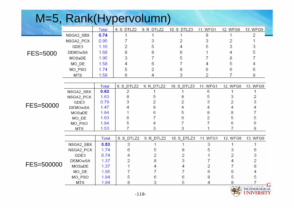
References to Algorithms in CEC07 papers
NSGAII_SBX: Sharma, Kumar et al.NSGAII_PCX: Kumar et al.GDE3: Kukkonen and Lampinen DEMOwSA: Zamuda et al. MOSaDE: Huang et al. MO_DE: Zielinski and LaurMO_PSO: Zielinski and LaurMTS: Tseng and Chen

-112-
CEC07 Function Sets
Three subsets2-objective functions3-objective functions5-objective functions
Comparison: Rank of the mean of the metric values from 25 runs

-113-
M=2, Rank(R indicator)
FES=5000
FES=50000
FES=500000

-114-
M=2, Rank(Hypervolumn)
FES=5000
FES=50000
FES=500000

-115-
M=3, Rank(R indicator)
FES=5000
FES=50000
FES=500000

-116-
M=3, Rank(Hypervolumn)
FES=5000
FES=50000
FES=500000

-117-
M=5, Rank(R indicator)
FES=5000
FES=50000
FES=500000
-118-
M=5, Rank(Hypervolumn)
FES=5000
FES=50000
FES=500000

-119-
CEC07 Summarized Results - Rank by IR2

-120-
CEC07 Summarized Results - Rank by HI

-121-
CEC07 Summarized Results - Rank by IR2 and HI

-122-
Rank (IR2 and ) on all test problemsFES=5000 FES=50000
FES=500000
HI

-123-
Acknowledgement
Our research into evolutionary algorithms in Singapore is financially supported by an A*Star (Agency for Science, Technology and Research), Singapore
Thanks to all past and current researchers working with me for their contributions. These slides show the results of their research efforts.