particle-based simulation of fluidstolga/pubs/particlefluidshires.pdfeurographics 2003 / p. brunet...

EUROGRAPHICS 2003 / P. Brunet and D. Fellner(Guest Editors)

Volume 22 (2003), Number 3

Particle-Based Simulation of Fluids

Simon Premože1, Tolga Tasdizen2, James Bigler2, Aaron Lefohn2 and Ross T. Whitaker2

1 Computer Science Department, University of Utah2 Scientific Computing and Imaging Institute, University of Utah

AbstractDue to our familiarity with how fluids move and interact, as well as their complexity, plausible animation of fluidsremains a challenging problem. We present a particle interaction method for simulating fluids. The underlyingequations of fluid motion are discretized using moving particles and their interactions. The method allows simula-tion and modeling of mixing fluids with different physical properties, fluid interactions with stationary objects, andfluids that exhibit significant interface breakup and fragmentation. The gridless computational method is suitedfor medium scale problems since computational elements exist only where needed. The method fits well into thecurrent user interaction paradigm and allows easy user control over the desired fluid motion.

1. Introduction

Fluids and our interactions with them are part of our ev-eryday lives. Due to our familiarity with fluid movement,plausible simulation of fluids remains a challenging prob-lem despite enormous improvements7, 6. Advances in com-putational fluid dynamics (CFD) often cannot be directlyapplied to computer graphics, because they have vastly dif-ferent goals. Visual effects for feature films call for veryhigh resolution simulations with very realistic appearanceand motion. In addition, control over motion and appearanceis necessary for artistic purposes such that physically impos-sible things become possible and that fluid motion is script-able for user’s specific needs. Foster and Fedkiw7 and En-right et al.6 showed that very realistic animation of water ispossible. Unfortunately, existing methods are computation-ally very expensive and very slow to use. While great strideshave been made to make fluid simulation more controllable7,these grid-based methods do not fit well with current user-interaction paradigm used in modelling and animation tools.Furthermore, large scale problems such as stormy seas re-quire large grids and are currently impractical to simulate.Also, multiphase flows, multiple fluids mixing, and sedi-mentary flows are not easy to model. Foster and Fedkiw7 andEnright et al.6 addressed some of the difficult problems withthe grid-based methods using a hybrid representation: frag-mentation and merging of fluids, numerical diffusion in con-vection computation, etc. There are alternative approaches togrid-based methods for simulating fluid flows: Large EddySimulation, vorticity confinement, vortex vethods, and par-

ticle methods. Large-Eddy Simulation (LES) adds an extraterm to the Navier-Stokes equations to model the transfer ofenergy from the resolved scales to the unresolved scales. Invortex methods, large time steps are allowed and computa-tional elements exist only where interesting flow occurs.

To address some of the deficiencies of the grid-basedmethods, we describe a particle interaction method for sim-ulation of fluids. The underlying equations of fluid motion(the Navier-Stokes equations) are discretized using mov-ing particles and their interactions. The particle method de-scribed is very simple and easy to implement. It fits betterinto current user-interaction paradigm and setting the sim-ulation and controlling it is easy and intuitive. The methodallows setting up the simulation (inflow and outflow bound-aries, obstacles, forces) at coarse resolution (small numberof large particles) to quickly preview the motion. Once theuser is satisfied with the overall motion of the fluid flow,the simulation is run at high resolution to produce the finalfluid motion. The computational elements (fluid particles)are only used in parts of the scene where they are requiredand number of computational elements can change duringthe course of the simulation. Therefore, if more detail is re-quired in part of the scene, more particles can be put there toget finer detail. The method can handle mixing fluids seam-lessly without special treatment, and multiphase flows wheremultiple fluids exist in liquid and gaseous form can also besimulated with minimal modifications. While particle-basedmethods have been presented in computer graphics literature

c© The Eurographics Association and Blackwell Publishers 2003. Published by BlackwellPublishers, 108 Cowley Road, Oxford OX4 1JF, UK and 350 Main Street, Malden, MA02148, USA.

Premože et al. / Particle-Based Simulation of Fluids

before, none of those methods dealt with incompressible flu-ids and water-like liquids.

Foster and Fedkiw7 pointed out that it is difficult to createa smooth surface out of particles. Many particles are neces-sary to obtain a smooth surface. While many different meth-ods can be used to create a surface from particles, we use alevel set PDE method to reconstruct the surface. The levelset surface is reconstructed on a grid whose resolution andcomputation are completely independent of the fluid simu-lation. On the other hand, for preview purposes, blending ofpotential fields around each particle can be used to give fastfeedback on how the surface might look.

While the grid-based methods described by Foster andFedkiw7 and Enright et al.6 provide impressive results, theparticle-based method could provide an alternative for simu-lation and animation of variety of fluids with different phys-ical properties while allowing user control and fast feedbackat coarse resolutions.

2. Background And Previous Work

Simulation of fluids and their motion in computer graph-ics has been attempted with a variety of methods. Webriefly overview methods relevant to the work presented inthis paper. Early methods were geared towards simplify-ing the computation by using Fourier synthesis18 or provid-ing specialized solution for a specific problem9, 25. Kass andMiller13 used height field to represent the fluid surface andused shallow water partial differential equations to describethe fluid motion. O’Brien and Hodgins22 also used a heightfield representation coupled with a particle system to rep-resent fluid motion with splashing that was missing in pre-vious methods. Foster and Metaxas8 realized the limitationof the height field representation and used a Marker-And-Cell (MAC) method11 to solve the Navier-Stokes equations.Massless marker particles are put into the computational gridand advected according to the velocity field to track the sur-face. Their method was a true 3D method and was thereforeable to simulate fluid pouring and splashing. Stam28 simu-lated fluids using a semi-Lagrangian convection that allowedmuch larger time-steps while being unconditionally stable.Foster and Fedkiw7 greatly improved the MAC method byusing the level set approach for tracking the fluid interface.Enright et al.6 further improved this method by introducingan improved method of tracking the water interface usingparticle level set and a new velocity extrapolation method.Enright et al.5 describe this thickened front tracking methodin more detail. Carlson et al. also utilized the MAC algo-rithm for animation of melting and solidifying objects1.

Alternative methods of simulation fluid motion weredescribed by using particle-based simulations. Miller andPearce19 simulate deformable objects with particle interac-tions based on the Lennard-Jones potential force. This forceis strongly repellent when particles are close together and

weakly attractive when particles are some distance apart.Terzopoulos et al.33 pairs particles together to better simu-late deformable objects. Tonnesen34 improves particle mo-tion by adding additional particle interactions based on heattransfer among particles.

Lucy17 introduced a flexible gridless particle methodcalled smoothed particle hydrodynamics (SPH) to simulateastrophysical problems including galaxial collisions and thedynamics of star formation. The fluid is modeled as a col-lection of particles, which move under the influence of hy-drodynamic and gravitational force. SPH has recently beenadapted to many relevant engineering problems, includingheat and mass transfer, molecular dynamics, and fluid andsolid mechanics. SPH is a flexible Lagrangian method20, 21

that can easily capture large interface deformation, breakingand merging, and splashing. Desbrun and Cani-Gascuel3 de-scribed a model of deformable surfaces and metamorphosiswith active implicit surfaces. SPH method was used to com-pute particles motion and particles were coated with a po-tential field. Desbrun and Cani improved the particle modelto simulate a variety of substances using a state equationto compute the dynamics of the substance2 . Adaptive sam-pling of particles improved the computational efficiency ofthe method by subdividing particles where substance under-goes large deformation, and merging particles in less activeareas. Stora et al.29 also used smoothed particles to solve thegoverning state equation for animated lava flows by couplingviscosity and temperature field.

While the SPH method is flexible, it can only solve com-pressible fluid flow. Several extensions have been proposedto allow simulation of incompressible fluids with SPH. Re-cently, another gridless particle method called the Moving-Particle Semi-Implicit (MPS) was developed that solves gov-erning Navier-Stokes equations for incompressible fluids14.The MPS method is capable of simulating a wide variety offluid flow problems including phase transitions, multiphaseflow, sediment-laden flows and elastic structures37, 15, 12. Thecomputational algorithm in this paper is based on the MPSmethod.

3. Gridless Particle Method

The Moving Particle Semi-implicit method is a Lagrangianmethod of computing fluid motion. Contrary to the grid-based Eulerian methods where physical quantities are com-puted on fixed points in space, the computational elementsin the MPS method are discrete number of particles of fluidfollowed in time. The MPS method is meshless. Given an ar-bitrary distribution of interpolation points, all problem vari-ables are obtained from values at these points through an in-terpolation function (kernel). Interpolation points and fluidparticles coincide.

GOVERNING EQUATIONS FOR INCOMPRESSIBLE

FLOW. The motion of a fluid can be described by the Navier-

c© The Eurographics Association and Blackwell Publishers 2003.


u Velocityr Positionr Distance between particlesre Interaction radiusd Number of space dimensionst Timedt Time stepw Weight functionµ Viscosityσ Surface tensionκ Surface curvatureρ Densityn0 Fluid particle density

Table 1: Notation and important terms used in the paper.

Stokes equations. If u is a velocity field of the fluid, the con-tinuity equation states that the mass m is constant:

∇·u = 0, (1)

and thus enforces the incompressibility of the fluid. The con-servation of momentum relates velocity and pressure:

∂u∂t

+ u ·∇u = −1ρ∇p + ν∇2u + f, (2)

where ρ is density of the fluid, p is the pressure, ν is the vis-cosity and f are forces. Other equations that describe molec-ular diffusion, surface tension, conservation of energy andmany other relationships could also be written for a givenfluid. Table 1 summarizes important terms and notation usedin this paper.

3.1. Particle Interactions

In particle methods, mass, momentum and energy conserva-tion equations are transformed to particle interaction equa-tions. All interactions between particles are limited to a fi-nite distance. The weight of interaction between two parti-cles that are distance r apart is

w(r) =

{ rer if 0 ≤ r ≤ re

0 if re ≤ r(3)

where r is the distance between two particles i and j,

r = |r j − ri|. (4)

If all particles are allowed to interact, the complexity isO(N2). In contrast, if interaction radius is restricted, thecomplexity is only O(NM), where M is the number of in-teracting particles24 within the radius of interaction re. Theparticle number density n can be computed as

〈n〉i = ∑j 6=i

w(|r j − ri|).

The number of particles in a unit volume is approximated bythe particle number density

〈ρn〉i =〈n〉i�

w(r)dv.

For an incompressible fluid, the fluid density must be con-stant: n0.

To solve the Navier-Stokes equations, differential opera-tors on particles must be defined. Let φ and u be arbitraryscalar and vector quantities. The gradient ∇φ is the averageof scalar gradient between particle i and neighboring particlej:

〈∇φ〉i =dn0 ∑

j 6=i

φ j −φi

|r j − ri|2(r j − ri)w(|r j − ri|). (5)

Similarly, the vector gradient ∇u is the average of vectorgradient between particle i and neighboring particle j:

〈∇ ·u〉i =dn0 ∑

j 6=i

(u j −ui) · (r j − ri)

|r j − ri|2w(|r j − ri|). (6)

The Laplacian operator ∇2 is derived from the concept ofdiffusion. It can be seen as if a fraction of a quantity at par-ticle i is distributed to neighboring particle j:

〈∇2φ〉i =2dλn0 ∑

j 6=i

(φ j −φi)w(|r j − ri|), (7)

where λ:

λ =

�V w(r)r2dv�

V w(r)dv. (8)

Note that this model does not require any spatial connec-tivity information. When particles move around no specialcare or reconfiguration is needed. Grid-based method suf-fer from numerical breakdown when computational meshgets tangled due to large interface deformations. Arbitrarymaterials and surfaces can all be represented with particles.Any complex boundaries and objects (stationary or moving)can be described with particle arrangements. This allows forsimulation of complex problems in a simple unified mannerwithout special cases.

3.2. MPS Method

The Navier-Stokes equations are solved by the semi-implicitMPS method. For every time step dt, the forces and viscos-ity in the momentum conservation equation are computedexplicitly. Temporary particle locations r∗ and velocities u∗

are computed from the positions rn and velocities rn fromthe previous time step n as follows:

u∗ = un +dtρ

(

µ∇2un + σ(κ ·n)n + ρg)

, (9)

and

r∗ = rn + u∗dt. (10)



The surface tension model and computation is described inAppendix A. After this step, the incompressibility of thefluid is temporarily violated. The temporary particle densityn∗ is not equal to n0. The particle density n∗ needs to bemodified by n′ such that the continuity equation is satisfied.The particle density n′ is related to modification of the ve-locity u′:

1dt

n′

n0 = ∇·u′. (11)

The modification velocity u′ is obtained from the implicitpressure term in the momentum conservation equation:

u′ = −dtρ∇pn+1. (12)

Note that this is the same as in the grid-based methods suchas MAC. By substituting equations 11 and 12 into

n0 = n∗ + n′, (13)

a Poisson equation for pressure is obtained:

〈∇2 pn+1〉i = −ρdt

〈n∗〉i −n0

n0 . (14)

The right hand side of equation 14 is analogous to the di-vergence of the velocity vector. Equation 14 is solved byusing the Laplacian differential operator and discretizing itinto a system of linear equations. The matrix representingthese linear equations is sparse and symmetric; therefore itcan be solved using the conjugate gradient method. Once thepressure pn+1 is computed, the correction velocity u′ alsobecomes known:

u′ = −dtρ〈∇pn+1〉. (15)

New particle velocities and positions that satisfy both con-servation of mass and momentum can then be updated:

un+1 = u∗ + u′ (16)

rn+1 = rn + un+1dt. (17)

BOUNDARY CONDITIONS. The particle density numberdecreases for particles on the free surface. A particle whichsatisfies a simple condition

〈n∗〉i < βn0, (18)

is considered on the free surface. In this paper, we useβ = 0.97. Intuitively, this makes sense because the weight-ing kernel will span the fluid interface. Pressure p = 0 (oratmospheric pressure, if applicable) is applied to these par-ticles on the free surface in the pressure calculation. Solidboundaries such as walls or other fixed objects are repre-sented by fixed particles. Velocities are always zero at theseparticles. Three layers of particles are used to represent fixedobjects to ensure that particle density number is computedaccurately. Note that there is no explicit collision detection

Algorithm 1 The Moving Particle Semi-Implicit (MPS) al-gorithm.

Initialize fluid: u0, r0

for each time step dtCompute forces and apply them to particles. Find temporaryparticle positions and velocities u∗, r∗

Compute particle number density n∗ using new particle loca-tions r∗

Set up and solve Poisson pressure equation using ConjugateGradient methodCompute velocity correction u′ from the pressure equationCompute new particle positions and velocities:un+1 = u∗ + u′

rn+1 = r∗ + u′dtend for

between particles. The pressure that is computed at fixed par-ticles essentially repels the fluid particles from the fixed ob-jects. Therefore, no special cases are therefore needed andarbitrary object-fluid configurations can be handled in thesame computation seamlessly.

The basic MPS algorithm is summarized in Algo-rithm 3.2.

DISADVANTAGES. It is worth noticing that the gridlessMPS method has several disadvantages. Since it is a La-grangian method, inflow and outflow of fluid is not allowed.However, it can be easily combined with the Eulerian ap-proach to handle inflow and outflow. We will describe a sim-ple hybrid method in subsection 3.3. Conservation of scalars(energy, etc.) is not guaranteed. If one truly cares about con-servation, the finite volume methods based on integrals inthe cells are good for conservation. Also, large aspect ratiois impossible at the moment. Note however that this is also aproblem for the most-advanced finite volume methods. Thebiggest disadvantage of using particle method is the questionof surface representation. We have particles that accuratelyrepresent the fluid motion and other interesting quantities,but for rendering the fluid a surface representation is needed.We describe the surface representation and extraction in sec-tion 4.

3.3. MPS-MAFL Method

As discussed in the previous subsection, one of the mainproblems with a purely Lagrangian approach is that inflowand outflow of fluid cannot be handled. Furthermore, localresolution enhancement is hard, because fluid particles movearound. If more particles are introduced to improve resolu-tion, they will soon move to different locations. In order toalleviate problems of purely Lagrangian method in the MPSmethod, a gridless hybrid method has been developed37 . Themethod consists of three steps:

1. Lagrangian Phase: the MPS method2. Reconfiguration Phase: particle positions are reconfig-

ured



PSfrag replacements

rLi 〈r〉i

∆r

Interpolation region

Figure 1: Directional local grid. A one-dimensional grid iscreated in the particle’s streamline direction. The quantitiesare only interpolated in the cut disk area. (After Heo et al.12)

3. Eulerian Phase: particle convection is computed on a one-dimensional grid

The Lagrangian phase is exactly the same as described in theMPS method. We denote the particle positions and velocitiesobtained after this phase as uL and rL. The reconfigurationphase and convection (Eulerian) phase are described next.

Reconfiguration Phase

In order to correctly handle inflow and outflow boundariesand deal with irregular distribution of particles, the particlepositions have to be reconfigured. The computation pointsare redistributed considering the boundaries. Points that be-long to a fixed boundary (fixed objects, walls, etc.) or inletor outlet boundary, should go back to their original positionsrn. The moving boundary can be traced through Lagrangianmotion of points describing the free surface without comput-ing the convection term: rn+1

s = rLs where subscript s denotes

that the point is on the surface. In practice, it is likely that thepoints on the surface will cluster together. To fix this prob-lem, we make sure that the particles on the moving bound-ary are an equal distance apart. The reconfiguration phaseis equivalent to remeshing in grid-based methods. However,it is much easier in the particle-based methods because onlythe particle locations need to be adjusted. Note that the num-ber of fluid particles can vary. Therefore, higher particle con-centration can be used in areas that require higher accuracy.

The computation point rn+1 at the new time step is deter-mined arbitrarily and the velocity of the computing point uc

is

uc =rn+1 − rn

dt. (19)

The convection velocity is then given by

ua =rL − rn

dt−

rn+1 − rn

dt= −

rn+1 − rL

dt. (20)

Eulerian Phase

After arbitrary convection velocity ua is computed, proper-ties at rn+1 are computed by interpolation of physical prop-erty f (flow velocity, temperature, etc.):

f (t + dt,rn+1i ) = f (t,rL

i −uai dt). (21)

If the number of computation points changes during the re-configuration phase, the physical quantity f is computed by

f (t + dt,rn+1i ) = f L(t,rL

o −uai dt), (22)

where rLo is the closest point to rn+1

i .

We follow a simple meshless advection method, MAFL,proposed by Yoon et al.37. Other convection methods32 caneasily be substituted if so desired. There are four stages inthe convection phase computation:

1. Generate a one-dimensional directional grid,2. Locally interpolate physical quantities,3. Apply any high-order convection scheme,4. Filter the result to prevent oscillatory solutions.

DIRECTIONAL GRID GENERATION. Because the fluidproperties are changing along the streamline (direction ofthe velocity vector), the convection problem is a one-dimensional problem if a grid is generated in the flow di-rection. Figure 1 shows the directional grid. The number ofgrid points used in computation depends on the convectiondifference scheme used.

LOCAL INTERPOLATION. At a local grid point, thephysical properties 〈 f 〉k are interpolated from the neighbor-ing computing points f L

j using the weight:

〈 f 〉k =∑ j f L

j w(|rLj −〈r〉k|, re,k)

∑ j w(|rLj −〈r〉k|, re,k)

for k = -2,-1,1. (23)

CONVECTION SCHEME. Any difference scheme canbe used in the convection phase. If the first order upwindscheme is applied to local grid points, only two points areconsidered:

f n+1i = f L

i −q( f Li −〈 f 〉−1),q =

|ua|dtdr

. (24)

The second order QUICK16 scheme uses four points (twoupstream and one downstream) and yields

f n+1i = f n

i −q(1

8f ni−2 −

7

8f ni−1 +

3

8f ni +

3

8f ni+1),q =

|ua|dt

dr. (25)

FILTERING. Higher order schemes often result in oscilla-tory solutions. A filtering scheme can be applied to preventovershooting and undershooting. Minimum and maximumlimits are computed at each time step and the interpolantsare bounded by them:

f n+1i ==

f n+1i min( f n

i ) ≤ f n+1i ≤ max( f n

i )

min( f ni ) f n+1

i < min( f ni )

max( f ni ) f n+1

i > max( f ni )

(26)

Higher order schemes can exhibit numerical instability ifthere is a large change in the number of particles and theirlocations.

The hybrid MPS-MAFL algorithm that allows arbitraryinflow and outflow of fluid, and arbitrary addition and



Algorithm 2 The hybrid MPS-MAFL algorithm.Initialize fluidfor each time step dt

Lagrangian phase: the same as MPS algorithm (Algorithm 1)Reconfiguration phase: determine the positions of computingpoints and convection velocitiesCreate a one-dimensional local grid in the streamline directionInterpolate physical properties within the particle neighbor-hood

end for

removal of computation points is summarized in Algo-rithm 3.3. The interested reader is referred to papers byHeo et al.12 and Koshizuka et al.15 to learn more about MPS-MAFL methods.

3.4. Multifluid Flow

It is straightforward to extend the MPS and MPS-MAFLmodels described in sections 3.2 and 3.3 for multifluid andmultiphase flows27. Let uξ,i denote the velocity of a fluidparticle i of type ξ, and rξ,i be the position of the fluid par-ticle. The temporary velocity u∗

ξ that includes the diffusion,gravity, and surface tension is similar to equation 9:

u∗ξ = un

ξ +dtρξ

{µξ∇2un

ξ + σξ(κξ ·nξ)n + ρξg}. (27)

Other forces acting on the fluid can be included. The im-plicit pressure computation is similar to the single fluid MPSmethod. If the density of mixing fluids is on the same orderof magnitude, the pressure computation is done in a singlestep as before. In order to avoid numerical instabilities whenmultiple fluids have drastically different densities (e.g. wa-ter and air), the pressure computation for each fluid is doneseparately. First, the pressure computation is performed as ifall particles are gas particles. In the second step, the com-puted pressure for gas particles is applied to the interface ofthe liquid particles. This is an iterative process: if the particlevelocity and position converge we proceed to next step, oth-erwise we repeat the pressure computation again until con-vergence.

4. Surface Reconstruction

In this section, we introduce the notation of level set meth-ods and discuss our approach to surface reconstruction fromparticles. Let x(t) be the set of points on a deforming surfaceat time t. We represent this deforming surface implicitly as

S = {x(t) | φ (x(t), t) = 0} , (28)

where φ : � 3 → � is the embedding function. Surfaces de-fined in this way divide a volume into two parts: inside(φ > 0) and outside (φ < 0). It is common to choose φ tobe the signed distance transform of S, or an approximationthereof. The motion of S is controlled indirectly by modi-fying φ with a PDE. This family of PDEs and the upwind

scheme for solving them on a discrete grid is the methods oflevel sets proposed by Osher and Sethian23. In this paper, weconsider level set PDEs of the form

∂φ(x)/∂t = −||∇φ|| (F (x)+ µH (x)) , (29)

where F is a force term , H is the mean curvature of thelevel set interface and µ defines the relative weights of thetwo terms. The mean curvature term guarantees the smooth-ness of the interface by favoring surfaces of smaller areaover surfaces of larger area26. The force term F is designedto make the level set interface track the moving particles.We fix µ = 1 for all of our experiments. Note that the set-ting of the parameter µ is a trade-off between overall surfacesmoothness and the capturing of surface features defined byparticle positions.

For a given frame, the particle simulation provides a setof particle locations, radii and velocities {ri, ri,ui}

Ni=1. Let

F be a sum over all the particles of a kernel function f , i.e.

F(x) = T +N

∑i=1

f (x,ri, ri,ui), (30)

where T is a constant threshold. Let di(x) denote the Eu-clidean distance from the center of particle i to the pointx in space. Since the particles have a finite size, if we de-fine fi(x) to be 1 for di(x) ≤ ri and 0 outside, then F repre-sents the number of particles at any point in space. If we alsochoose T = −0.5, the points in space that satisfy F = 0 willapproximately represent the surface defined by the particles.However, this binary choice for f leads to a very rough look-ing surface, and the individual particles are easily recogniz-able in the reconstruction. The curvature smoothing term in(equation 29) can not compensate for this large-scale rough-ness. What is needed is a smoother choice for f that providesan interpolation between particles. Consider the following

fi(x) =1

1 + |di(x)/ri|k, (31)

where k = 2. This function falls off smoothly as the distanceto the particle increases, and is well-behaved as d → 0. Be-cause, f > 0 for di(x) > ri, F accumulates to larger quanti-ties than with the previous case. This necessatiates choosinga lower T value; we find that T =−2 is suitable. We also ex-perimented with k = 1 and k > 2, but these choices resultedin oversmoothing and not enough interpolation, respectively.

The interpolation obtained from (equation 31) is isotropic;therefore, it has a thickening effect on the surface due to in-terpolation in the direction perpendicular to the surface. Afurther modification can be made to solve this problem byallowing more interpolation in the physical surface tangentplane, and less interpolation perpendicular to this plane. Weuse the assumption that the velocities of the particles will beapproximately in the tangent plane. Let dv

i (x) and d⊥i (x) be



defined as :

dvi (x) =

∣

∣

∣

∣

(x− ri) ·ui

‖ ui ‖

∣

∣

∣

∣

, d⊥i (x) =

= ‖ (x− ri)− dvi

ui

‖ ui ‖‖ .

Let smax be the largest particle speed for the given frame.Then, we define the modified distance to a particle as

di(x) =

(

1−‖ ui ‖

2smax

)

dvi (x)+

(

1 +‖ ui ‖

2smax

)

d⊥i (x). (32)

Using this definition of distance in (equation 31) has theeffect of elongating the influence of a particle along its ve-locity vector and shrinking it in all other directions.

The surface reconstruction algorithm starts with the parti-cle information for the first frame. Before starting to eval-uate (equation 29), we need an initialization for φ. Aftercomputing F for the first frame, the initialization is obtainedfrom F = 0. Then, we iterate (equation 29) using an upwind,sparse-field implementation35 until convergence. The com-putation only occurs in grid cells that are on or near the sur-face. Convergence is reached when the change to φ per timestep falls below a pre-determined threshold. At this point,we save the state of the surface for generating the anima-tion. Then, F is constructed for the particle information con-tained in the next frame, and we continue iterating (equa-tion 29) without reinitialization. In other words, the surfaceresult from the previous frame acts as the initialization. Thisapproaach guarantees the continuity of the surface modelsproduced for consecutive frames. Note that the level set sur-face reconstruction step is solved on a grid whose resolutionis completely independent from the fluid simulation. Oncethe fluid simulation is computed, the surface reconstructionis done at arbitrary resolution.

5. Results and Discussion

The MPS and MPS-MAFL methods described in this pa-per methods are straighforward to implement. For efficientcomputation, a spatial data structure that quickly finds par-ticles in a neighborhood is desired although not necessary.The Poisson pressure equation can be efficiently solved witha Conjugate Gradient (CG) method. In our implementation,we use the CG method with an Incomplete Cholesky precon-ditioner. We use the SparseLib++ library4 for computing thePoisson pressure equation.

We show several examples of fluid simulation computedwith the MPS and MPS-MAFL methods. All simulationsand rendering were performed on a Pentium IV 1.7 Ghz with512 Mb of memory running Linux operating system. Videosof animations discussed in this sections accompany this pa-per.

The computational method is fairly efficient and allowssimulating about 10,000 particles per timestep per second.This is fast enough to get an instantaneous feedback onwhether the fluid simulation will run as desired. After we

set up the scene (objects, obstacles, forces, fluid properties)and initialize fluid particles, we run the fluid simulation atlow resolution to get feedback. After we set all simulationparameters (particle size, interaction radius, etc.) and forces(gravity, drag, surface tension, etc.), the final simulation isrun at high resolution. The main bottleneck in the compu-tation is the Poisson pressure equation computation and thecomputation time ultimately depends on the number of par-ticles in the simulation. As a part of future work, it would bebeneficial to parallelize the Conjugate Gradient algorithm tofurther speed up computation time on parallel architectures.

Corridor Flood

We simulated a simple flood in an underground corridor. Wemodeled the corridor with a small number of polygons andconverted the polygonal scene into the particle representa-tion. Each polygon was represented with three layers of fixedparticles. The inflow of water was simulated by positioninga virtual square inflow boundary that was turned on for ashort period of time. This could also be simulated as a wa-ter column collapse. The total number of fluid particles inthe scene is about 100,000. The only force acting on parti-cles was gravity. Surface tension was not included in thissimulation. The computation time for the final simulationwas about 3 minutes per frame. Surface reconstruction took10 minutes per frame (volume size 459x74x374). Figure 2shows several frames from the simulation. The final sur-face was rendered using a Monte Carlo path tracer with 10area light sources. The rendering time per frame was about20 minutes. Since the MPS method is fully Lagrangian, thecomputational elements (fluid particles) were only presentin the part of the scene where they were needed. Note thatbecause the corridor is L-shaped, this provides some compu-tational savings over the grid-based methods. In grid-basedapproaches, about 70 percent of the space would be wasted.A larger grid would be needed to accommodate the computa-tion, therefore yielding larger computation time and memoryrequirements.

Box Filling

In this simulation, we fill a box with a fluid that is beingpoured from a source with three nozzles. The fluid does notfall directly into the box. A polygonal obstacle set near thetop of the box at an angle obstructs the flow. The fluidsfrom the nozzles first hit the obstacle surface and then theside of the box. The fluid was simulated with about 150,000fluid particles. The simulation time is about 4 minutes perframe. Gravity, surface tension and drag force were actingupon fluid particles during the simulation. The fluids fromthe three nozzles have the same physical properties. Surfacereconstruction took 30 minutes per frame (volume size 197 x283 x 256). Figure 3 shows several frames from the box fill-ing simulation. The example animation was being rendered



Figure 2: Corridor flood simulation. The fluid motion issimulated by 100,000 fluid particles. The simulation time isabout 3 minutes per frame.

with a raytracer. Approximate rendering time was about 5minutes per frame.

Mixing fluids

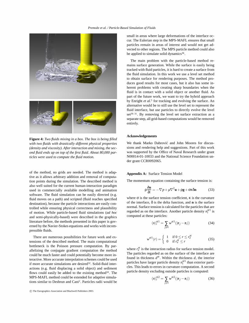
In this simulation, we fill a box with two fluids that havevery different densities and viscosities. First, we start fill-ing the box with a water-like fluid. After some time, westart filling the box with the second oil-like fluid. The flu-ids start interacting and mixing. The second fluid ends ontop of the first fluid as expected from the physical propertiesof the fluids. Gravity and surface tension were applied toboth fluids. About 80,000 fluid particles represent both flu-ids. The simulation time was 3 minutes per frame. Surfacereconstruction took 10 minutes per frame per fluid (volumesize 245x245x274). Figure 4 shows three frames from thissimulation. Observe the mixing and interactions between thetwo fluids. The images were being rendered with a raytracer.Approximate rendering time was 5 minutes per frame. Thesecond-fluid has oil-like physical properties. For visualiza-tion purposes we rendered this fluid opaquely to show theseparation between the two fluids. Some artefacts (e.g. round

Figure 3: A source with three nozzles filling a box. The fluidmotion is simulated by 150,000 fluid particles. The fluid isbeing emitted from three nozzles that hit an obstacle surfaceset near the top of the box.

boundary, non-perfectly smooth surface) resulting from thesurface reconstruction are visible.

6. Conclusion

We described a particle-based method for simulation fluidmotion. It is based on a particle discretization of the differ-ential operators to solve the Navier-Stokes equations. It issuited for simulating a wide variety of fluid flows includingmultifluids, multiphase flows and medium scale problemssuch as the corridor flood. Because of the Lagrangian nature



Figure 4: Two fluids mixing in a box. The box is being filledwith two fluids with drastically different physical properties(density and viscosity). After interaction and mixing, the sec-ond fluid ends up on top of the first fluid. About 80,000 par-ticles were used to compute the fluid motion.

of the method, no grids are needed. The method is adap-tive as it allows arbitrary addition and removal of computa-tion points during the simulation. The described method isalso well suited for the current human-interaction paradigmused in commercially available modelling and animationsoftware. The fluid simulation can be easily directed (e.g.fluid moves on a path) and scripted (fluid reaches specifieddestination), because the particle interactions are easily con-trolled while ensuring physical correctness and plausibilityof motion. While particle-based fluid simulations (ad hocand semi-physically-based) were described in the graphicsliterature before, the methods presented in this paper is gov-erned by the Navier-Stokes equations and works with incom-pressible fluids.

There are numerous possibilities for future work and ex-tensions of the described method. The main computationalbottleneck is the Poisson pressure computation. By par-allelizing the conjugate gradient computation the methodcould be much faster and could potentially become more in-teractive. More accurate interpolation schemes could be usedif more accurate simulations are desired32. Solid-fluid inter-actions (e.g. fluid displacing a solid object) and sedimentflows could easily be added to the existing method10. TheMPS-MAFL method could be extended for adaptive simula-tions similar to Desbrun and Cani2. Particles radii would be

small in areas where large deformations of the interface oc-cur. The Eulerian step in the MPS-MAFL ensures that smallparticles remain in areas of interest and would not get ad-vected to other regions. The MPS particle method could alsobe applied to simulate solid dynamics36.

The main problem with the particle-based method re-mains surface generation. While the surface is easily beingtracked with fluid particles, it is hard to create a surface fromthe fluid simulation. In this work we use a level set methodto obtain surface for rendering purposes. The method pro-duces good results for most cases, but it also has some in-herent problems with creating sharp boundaries when thefluid is in contact with a solid object or another fluid. Aspart of the future work, we want to try the hybrid approachby Enright et al.5 for tracking and evolving the surface. Analternative would be to still use the level set to represent thefluid interface, but use particles to directly evolve the levelset30, 31. By removing the level set surface extraction as aseparate step, all grid-based computations would be removedentirely.

Acknowledgements

We thank Marko Dabrovic and John Moores for discus-sions and rendering help and suggestions. Part of this workwas supported by the Office of Naval Research under grantN00014-01-10033 and the National Science Foundation un-der grant CCR0092065.

Appendix A: Surface Tension Model

The momentum equation containing the surface tension is:

ρ ∂u∂t

= −∇p + µ∇2u+ ρg + σκδn (33)

where σ is the surface tension coefficient, κ is the curvatureof the interface, δ is the delta function, and n is the surfacenormal. Surface tension is calculated for the particles that areregarded as on the interface. Another particle density nst1

i iscomputed at these particles:

〈n〉st1i = ∑

j 6=i

wst1(|r j − ri|) (34)

wst1(r) =

{

1 if 0 ≤ r ≤ rste

0 if rste ≤ r

(35)

where rste is the interaction radius for surface tension model.

The particles regarded as on the surface of the interface arefound in thickness dst . Within the thickness d, the interiorparticles have larger particle density nst1

i than exterior parti-cles. This leads to errors in curvature computation. A secondparticle density excluding outside particles is computed:

〈n〉st2i = ∑

j 6=i

wst2(|r j − ri|) (36)



wst2(r) =

{

1 if 0 ≤ r ≤ rste and nst1

j > nst1i

0 otherwise(37)

The curvature of the interface is then computed as:

κ =1R

=2cosθ

rste

(38)

2θ =nst2

i

nst10

π, (39)

where nst10 is constant and is computed when the interface is

flat (curvature is zero).

Appendix B: Drag Force Model

The drag force due to the permeable layer is:

f = −3

4

CD

d0|ui|ui (40)

wu(r) =

{

1/∑ wu(r) if r ≤ αd0

0 if r > αd0(41)

ui = ∑u jwu(|ri j |), (42)

where CD is drag coefficient, ui is spatially averaged veloc-ity of neighborhood particles, α is model constant and d0 isdiameter of a fluid particle.

References

1. Mark Carlson, Peter J. Mucha, R. Brooks Van Horn III, and Greg Turk. Meltingand flowing. In ACM SIGGRAPH Symposium on Computer Animation, 2002.

2. Mathieu Desbrun and Marie-Paule Cani. Space-time adaptive simulation of highlydeformable substances. Technical report, INRIA, 19990.

3. Mathieu Desbrun and Marie-Paule Cani-Gascuel. Active implicit surface for ani-mation. In Graphics Interface, 1998.

4. J. Dongarra, A. Lumsdaine, R. Pozo, and K. Remington. A Sparse Matrix Libraryin C++ for High Performance Architectures. In Proceedings of the Second ObjectOriented Numerics Conference, pages 214–218, 1994.

5. D. Enright, R. Fedkiw, J. Ferziger, and I. Mitchell. A hybrid particle level setmethod for improved interface capturing. J. Comput. Phys., (183):83–116, 2002.

6. Douglas P. Enright, Stephen R. Marschner, and Ronald P. Fedkiw. Animation andrendering of complex water surfaces. ACM Transactions on Graphics, 21(3):736–744, July 2002.

7. Nick Foster and Ronald Fedkiw. Practical animation of liquids. In Proceedings ofACM SIGGRAPH 2001, pages 23–30, August 2001.

8. Nick Foster and Demitri Metaxas. Realistic animation of liquids. In GraphicsInterface ’96, pages 204–212, 1996.

9. Alain Fournier and William T. Reeves. A simple model of ocean waves. In Com-puter Graphics (SIGGRAPH ’86 Proceedings), volume 20, pages 75–84, 1986.

10. Hitoshi Gotoh, Tomoki Shibahara, and Tetsuo Sakai. Sub-particle-scale turbulencemodel for the MPS method. Computational Fluid Dynamics Journal, 9(4):339–347, 2001.

11. F. H. Harlow and J. E. Welch. Numerical calculation of time-dependent viscousincompressible flow of fluid with a free surface. The Physics of Fluids, 8:2182–2189, 1965.

12. S. Heo, S. Koshizuka, and Y. Oka. Numerical analysis of boiling on heat-fluxand high subcoling condition using MPS-MAFL. Comput. Fluid Dynamics J.,45:2633–2642, 2002.

13. Michael Kass and Gavin Miller. Rapid, stable fluid dynamics for computer graph-ics. In Forest Baskett, editor, Computer Graphics (SIGGRAPH ’90 Proceedings),volume 24, pages 49–57, August 1990.

14. S. Koshizuka, H. Tamako, and Y. Oka. A particle method for incompressible vis-cous flow with fluid fragmentation. Comput. Fluid Dynamics J., 29(4), 1996.

15. S. Koshizuka, H. Y. Yoon, D. Yamashita, and Y. Oka. Numerical analysis of naturalconvection in a square cavity using MPS-MAFL. Comput. Fluid Dynamics J.,30(8):485–494, 2000.

16. B. P. Leonard. A stable and accurate convective modelling procedure based onquadratic upstream interpolation. Comp. Methods Appl. Mech. Eng., 19:59–98,1979.

17. L. B. Lucy. A numerical approach to the testing of the fission hypothesis. TheAstronomical Journal, 82(12):1013–1024, Dec 1977.

18. G. A. Mastin, P. A. Watterberg, and J. F. Mareda. Fourier synthesis of ocean scenes.IEEE Computer Graphics and Applications, 7(3):16–23, March 1987.

19. Gavin Miller and Andrew Pearce. Globular dynamics: A connected particle systemfor animating viscous fluids. Computers and Graphics, 13(3):305–309, 1989.

20. J. J. Monaghan. Smoothed particle hydrodynamics. Ann. Rev. Astron. Astrophys.,30(2):543–574, 1992.

21. J. J. Monaghan. Simulating free surface flows with SPH. Journal of ComputationalPhysics, (110):399–406, 1994.

22. J. F. O’Brien and J. K. Hodgins. Dynamic simulation of splashing fluids. In Com-puter Animation ’95, pages 198–205, April 1995.

23. S. Osher and J. Sethian. Fronts propagating with curvature-dependent speed: Algo-rithms based on Hamilton-Jacobi formulations. Journal of Computational Physics,79:12–49, 1988.

24. Allen M. P. and Tildesley D. J. Computer Simulation of Liquids. Clarendon Press,Oxford, 1987.

25. Darwyn R. Peachey. Modeling waves and surf. In Computer Graphics (SIGGRAPH’86 Proceedings), volume 20, pages 65–74, 1986.

26. Guillermo Sapiro. Geometric Partial Differential Equations and Image Analysis.Cambridge University Press, 2001.

27. N. Shirakawa, H. Horie, Y. Yamamoto, and S. Tsunoyama. Analysis of the voiddistribution in a circular tube with the two-fluid particle interaction model. Journalof Nuclear Science and Technology, 38(6):293–402, June 2001.

28. Jos Stam. Stable fluids. In Proceedings of SIGGRAPH 99, pages 121–128, August1999.

29. D. Stora, P.O. Agliati, M.P. Cani, F. Neyret, and J.D. Gascuel. Animating lavaflows. In Graphics Interface, Kingston, Canada, June 1999.

30. John Strain. Semi-Lagrangian Methods for Level Set Equations. J. Comput. Phys.,151:498–533, 1999.

31. John Strain. A Fast Modular Semi-Lagrangian Method for Moving Interfaces. J.Comput. Phys., 161:512–536, 2000.

32. Nobuatsu Tanaka. Hamiltonian particle dunamics, CIVA-particle method and sym-plectic upwind scheme. Computational Fluid Dynamics Journal, 9(4):384–393,2001.

33. Demetri Terzopoulos, John Platt, and Kurt Fleischer. Heating and melting de-formable models (from goop to glop). In Proceedings of Graphics Interface ’89,pages 219–226, June 1989.

34. David Tonnesen. Modeling liquids and solids using thermal particles. In Proceed-ings of Graphics Interface ’91, pages 255–262, June 1991.

35. Ross T. Whitaker. Algorithms for implicit deformable models. In Fifth Interna-tional Conference on Computer Vision. IEEE Computer Society Press, 1995.

36. S. Koshizuka Y. Chikazawa and Y. Oka. A particle method for elastic andvisco-plastic structures and fluid-structure interactions. Computational Mechan-ics, 27:97–106, 2001.

37. H. Y. Yoon, S. Koshizuka, and Y. Oka. A particle gridless hybrid method for in-compressible flows. Int. J. Numer. Meth. Fluids, 29(4), 1996.


particle-based simulation of fluidstolga/pubs/particlefluidshires.pdfeurographics 2003 / p. brunet...

Documents