partial entrainment of gravel bars during floods

Partial entrainment of gravel bars during floods

Christopher P. Konrad

U.S. Geological Survey, Tacoma, Washington, USA

Derek B. Booth and Stephen J. Burges

Department of Civil and Environmental Engineering, University of Washington, Seattle, Washington, USA

David R. Montgomery

Department of Earth and Space Sciences, University of Washington, Seattle, Washington, USA

Received 6 August 2001; revised 14 January 2002; accepted 24 January 2002; published 11 July 2002.

[1] Spatial patterns of bed material entrainment by floods were documented at sevengravel bars using arrays of metal washers (bed tags) placed in the streambed. The observedpatterns were used to test a general stochastic model that bed material entrainment is aspatially independent, random process where the probability of entrainment is uniformover a gravel bar and a function of the peak dimensionless shear stress t*0 of the flood. Thefraction of tags missing from a gravel bar during a flood, or partial entrainment, had anapproximately normal distribution with respect to t*0 with a mean value (50% of the tagsentrained) of 0.085 and standard deviation of 0.022 (root-mean-square error of 0.09).Variation in partial entrainment for a given t*0 demonstrated the effects of flowconditioning on bed strength, with lower values of partial entrainment after intermediatemagnitude floods (0.065 < t*0 < 0.08) than after higher magnitude floods. Although theprobability of bed material entrainment was approximately uniform over a gravel barduring individual floods and independent from flood to flood, regions of preferentialstability and instability emerged at some bars over the course of a wet season. Deviationsfrom spatially uniform and independent bed material entrainment were most pronouncedfor reaches with varied flow and in consecutive floods with small to intermediatemagnitudes. INDEX TERMS: 1815 Hydrology: Erosion and sedimentation; 1821 Hydrology: Floods;

1869 Hydrology: Stochastic processes; KEYWORDS: sediment transport, bed material entrainment, disturbance,

gravel bars, stochastic model

1. Introduction

[2] The entrainment of streambed material is a principalecohydrologic process that influences fluvial sedimenttransport rates and the diversity and abundance of benthosin stream ecosystems. The spatial extent of bed materialentrainment during a flood varies from a few grains to allof the material forming the bed surface, with correspond-ingly vast differences in sediment transport rates andbiological consequences. Our objectives are to develop arelation between the fraction of a streambed surfaceentrained during a flood, which we refer to as partialentrainment, and the peak dimensionless shear stress dur-ing the flood and to evaluate whether bed material entrain-ment can be represented as a spatially independent,random process where the probability of entrainment isuniform over a gravel bar.[3] Spatial distributions of the shear stress applied by

streamflow t and the critical shear stress of bed materialtcr produce partial entrainment when t exceeds tcr atsome but not all locations on the bed [Lane and Kalinske,1940; Grass, 1970]. Field studies using tracer particles andbed load samplers have demonstrated that partial entrain-

ment rather than complete mobilization of a streambedprevails during most floods in gravel bed streams[Andrews and Erman, 1986; Ashworth and Ferguson,1989; Andrews, 1994]. Flume investigations of the initialmotion and transport rates of sediments also have docu-mented the partial entrainment of sand and gravel beds[Gilbert, 1914; Gessler, 1970; Grass, 1970; Wilcock andMcArdell, 1997]. In a study of six gravel bed streams,Lisle et al. [2000] conclude that only a limited portion ofthe streambed actively contributes sediment to bed loadtransport at bank-full discharge and that differences in thearea of active transport reflects differences in sedimentsupply between the streams.[4] Partial entrainment has been described as a stochastic

process because there is a finite probability that the texceeds tcr at any location on a streambed due to temporalfluctuations in stream velocity [Einstein, 1942]. In a sto-chastic bed load transport model, Einstein [1942, 1950]used a Gaussian distribution to calculate the ‘‘instantane-ous’’ probability of entrainment, based on a diffusion modelfor the spatial correlation of fluid velocity in turbulent flow[Taylor, 1935]. To calculate transport rates over larger reachscales encompassing many individual particles, Einsteinequated the area entrained by streamflow to the probabilityof entrainment. Lane and Kalinske [1940] and Grass [1970]recognized partial entrainment as the area of streambed

Copyright 2002 by the American Geophysical Union.0043-1397/02/2001WR000828$09.00

9 - 1

WATER RESOURCES RESEARCH, VOL. 38. NO. 7, 10.1029/2001WR000828, 2002

where t exceeds tcr. Using a flume with a sand bed, Grassfound that t had positively skewed, unimodal probabilitydistributions, while tcr had relatively uniform probabilitydistributions. Although Kirchner et al. [1990] described thecomponents influencing tcr (i.e., friction angle, projection,and exposure) as having widely distributed values for awater-worked bed, they did not suggest a general form forthe distribution of tcr.[5] In contrast to efforts to determine the individual

distributions of t and tcr , observations of bed mobility influmes have been used to assess their joint distribution interms of the probability of entrainment or partial entrain-ment. Gessler [1970] found that the cumulative probabilitythat a particle remained on the bed surface during clear-water flume runs was normally distributed with respect tot50i/t, where t50i is the shear stress that entrains 50% of thesurface particles of size class i. In a sediment-recirculatingflume, Wilcock [1997] observed that the equilibrium mobilefraction Y of any size class i had a log normal distributionwith respect to t/t50i. In both of these examples, the partialentrainment of a mixed sediment depends on the relativemobility of each particle size class.[6] The applicability of entrainment theory [White, 1940;

Komar and Li, 1986] or empirical results from flumeexperiments [see also Little and Mayer, 1976; Fenton andAbbot, 1977; Ikeda and Iseya, 1988] to gravel bed streamsis difficult to confirm because of sparse data on the spatialdistributions of t and tcr and a lack of control on theprocesses and conditions in the field. However, if theprobability of bed material entrainment is spatially uniformand independent over time, it could be estimated for agravel bed stream with few data, facilitating the assessmentof the sediment supply for bed load transport or the spatialextent of disturbance during floods.

2. Field Sites

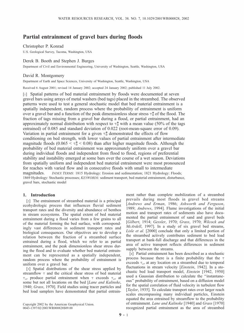
[7] Spatial patterns of bed material entrainment weredocumented during floods at seven gravel bars in threestreams (Jenkins, May, and Swamp Creeks) in the PugetLowland, Washington (Figure 1). The basins draining tothese creeks have intermediate levels of urban developmentbut contrasting physiographic conditions and differenthydrologic characteristics. As a result, these streams spanmuch of the range of conditions that influence the relativesediment supply and transport capacity of gravel bedstreams in the Puget Lowland region.[8] All sites are in straight sections of pool-riffle or plane

bed reaches [Montgomery and Buffington, 1997] with mid-channel or transverse gravel bars (of low amplitude in planebed reaches) where the particle size distributions of bedmaterial are relatively homogeneous and hydraulic condi-tions are relatively uniform (Table 1). Gravel bars aredefined here as local in-channel deposits of gravel that riseabove the mean profile of the bed surface [Church andJones, 1982].[9] Jenkins Creek drains a 37-km2 basin on a glacial

outwash plain. The mean discharge rate during water years(WY) 1989–1998 was 1.1 m3 s�1 at the King Countygage near its mouth. Storm flow recession is gradual, andbase flows are high relative to other streams in the region.[10] The supply of sediment to Jenkins Creek is limited

by the presence of lakes and wetlands in the channel

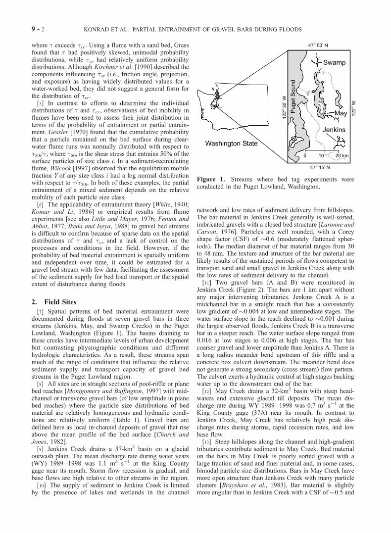
network and low rates of sediment delivery from hillslopes.The bar material in Jenkins Creek generally is well-sorted,imbricated gravels with a closed bed structure [Laronne andCarson, 1976]. Particles are well rounded, with a Coreyshape factor (CSF) of �0.6 (moderately flattened spher-iods). The median diameter of bar material ranges from 30to 48 mm. The texture and structure of the bar material arelikely results of the sustained periods of flows competent totransport sand and small gravel in Jenkins Creek along withthe low rates of sediment delivery to the channel.[11] Two gravel bars (A and B) were monitored in

Jenkins Creek (Figure 2). The bars are 1 km apart withoutany major intervening tributaries. Jenkins Creek A is amidchannel bar in a straight reach that has a consistentlylow gradient of �0.004 at low and intermediate stages. Thewater surface slope in the reach declined to �0.001 duringthe largest observed floods. Jenkins Creek B is a transversebar in a steeper reach. The water surface slope ranged from0.016 at low stages to 0.006 at high stages. The bar hascoarser gravel and lower amplitude than Jenkins A. There isa long radius meander bend upstream of this riffle and aconcrete box culvert downstream. The meander bend doesnot generate a strong secondary (cross stream) flow pattern.The culvert exerts a hydraulic control at high stages backingwater up to the downstream end of the bar.[12] May Creek drains a 32-km2 basin with steep head-

waters and extensive glacial till deposits. The mean dis-charge rate during WY 1989–1998 was 0.7 m3 s�1 at theKing County gage (37A) near its mouth. In contrast toJenkins Creek, May Creek has relatively high peak dis-charge rates during storms, rapid recession rates, and lowbase flow.[13] Steep hillslopes along the channel and high-gradient

tributaries contribute sediment to May Creek. Bed materialon the bars in May Creek is poorly sorted gravel with alarge fraction of sand and finer material and, in some cases,bimodal particle size distributions. Bars in May Creek havemore open structure than Jenkins Creek with many particleclusters [Brayshaw et al., 1983]. Bar material is slightlymore angular than in Jenkins Creek with a CSF of �0.5 and

Figure 1. Streams where bed tag experiments wereconducted in the Puget Lowland, Washington.

9 - 2 KONRAD ET AL.: PARTIAL ENTRAINMENT OF GRAVEL BARS DURING FLOODS

with median diameters ranging from 31 to 50 mm. Thetexture and structure of bed material in May Creek are likelya consequence of a large sediment supply and short durationof flows that are able to sort bed material.[14] Three gravel bars (A, B, and Z) were monitored in

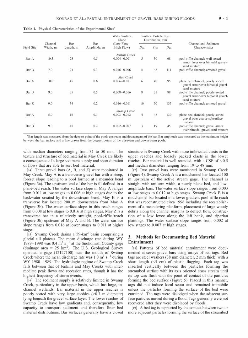
May Creek. May A is a transverse gravel bar with a steep,foreset slope leading to a pool formed at a meander bend(Figure 3a). The upstream end of the bar is ill defined in aplane-bed reach. The water surface slope in May A rangesfrom 0.011 at low stages to 0.006 at high stages due to thebackwater created by the downstream bend. May B is atransverse bar located 200 m downstream from May A(Figure 3b). The water surface slope in this reach rangesfrom 0.008 at low stages to 0.016 at high stages. May Z is atransverse bar in a relatively straight, pool-riffle reach(Figure 3b) upstream of May A and B. The water surfaceslope ranges from 0.016 at lower stages to 0.011 at higherstages.[15] Swamp Creek drains a 59-km2 basin comprising a

glacial till plateau. The mean discharge rate during WY1989–1998 was 0.4 m3 s�1 at the Snohomish County gage(drainage area = 25 km2). The U.S. Geological Surveyoperated a gage (12127100) near the mouth of SwampCreek where the mean discharge rate was 1.0 m3 s�1 duringWY 1980–1989. The hydrologic regime of Swamp Creekfalls between that of Jenkins and May Creeks with inter-mediate peak flows and recession rates, though it has thehighest frequency of storm events.[16] The sediment supply is relatively limited in Swamp

Creek, particularly in the upper basin, which has large, in-channel wetlands. Bar material in the upper reaches ispoorly sorted with very large cobbles (>0.3 m diameter)lying beneath the gravel surface layer. The lower reaches ofSwamp Creek have low gradients and, consequently, lowcapacity to transport sediment and therefore finer bedmaterial distributions. Bar surfaces generally have a closed

structure in Swamp Creek with more imbricated clasts in theupper reaches and loosely packed clasts in the lowerreaches. Bar material is well rounded, with a CSF of �0.5and median diameters ranging from 19 to 48 mm.[17] Two gravel bars were monitored in Swamp Creek

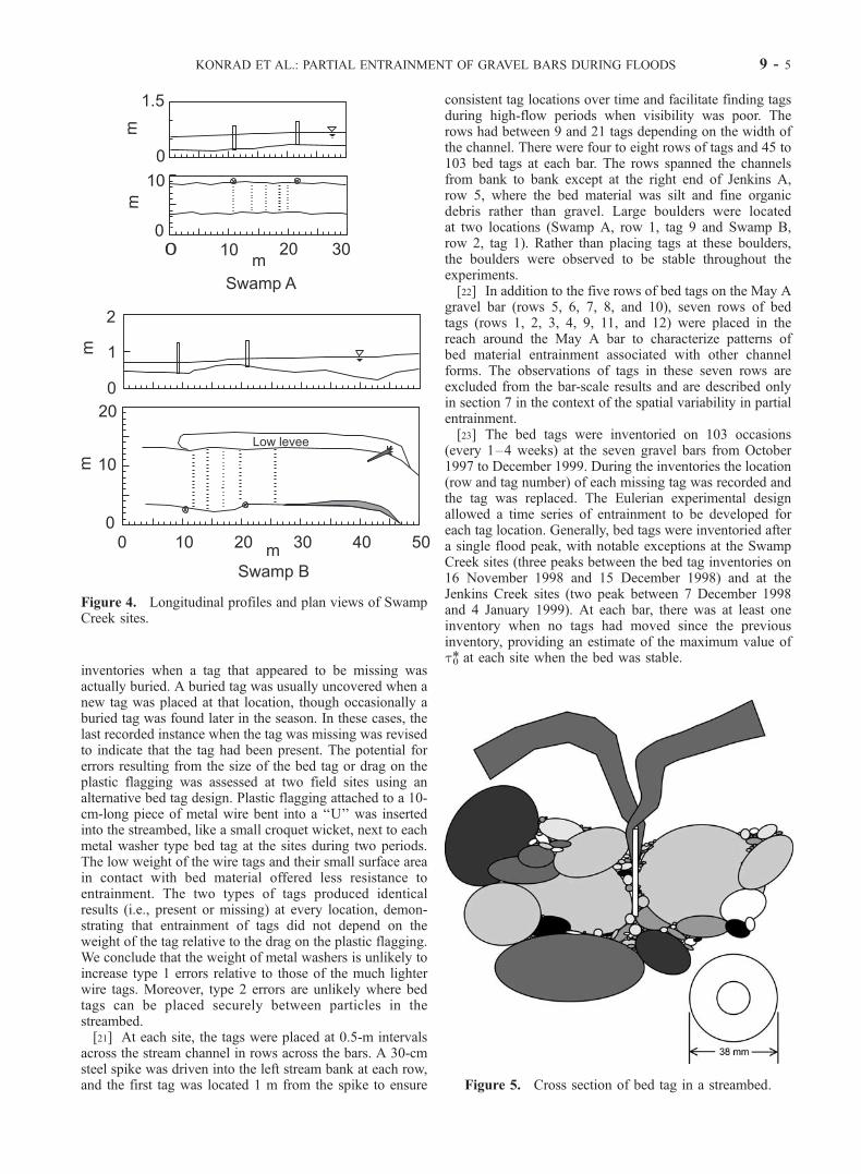
(Figure 4). Swamp Creek A is a midchannel bar located 100m upstream of the active stream gage. The channel isstraight with uniform width, a nearly plane bed, and low-amplitude bars. The water surface slope ranges from 0.003at low stages to 0.012 at high stages. Swamp Creek B is amidchannel bar located in a lower gradient pool-riffle reachthat was reconstructed circa 1996 including the reestablish-ment of a meandering planform, placement of large woodydebris along the channel margins to deflect flow, construc-tion of a low levee along the left bank, and riparianplantings. The water surface slope ranges from 0.002 atlow stages to 0.007 at high stages.

3. Methods for Documenting Bed MaterialEntrainment

[18] Patterns of bed material entrainment were docu-mented at seven gravel bars using arrays of bed tags. Bedtags are steel washers (38 mm diameter, 2 mm thick) with ashort length (<5 cm) of plastic flagging. Each tag wasinserted vertically between the particles forming thestreambed surface with its axis oriented cross stream untilits top was flush with the point of contact of the particlesforming the bed surface (Figure 5). Placed in this manner,tags did not induce local scour and remained immobileunless the particles forming the surface of the bed wereentrained. The tags were dislodged when the adjacent sur-face particles moved during a flood. Tags generally were notrecovered after they were displaced by floods.[19] A bed tag is supported by the contact between two or

more adjacent particles forming the surface of the streambed

Table 1. Physical Characteristics of the Experimental Sitesa

Field SiteChannelWidth, m

BarLength, m

BarAmplitude, m

Water SurfaceSlope

(Low Flow–High Flow)

Surface Particle SizeDistribution, mm

Channel and SedimentCharacteristicsD10 D50 D90

Jenkins CreekBar A 10.5 23 0.5 0.004–0.001 5 30 68 pool-riffle channel; well-sorted

armor layer over bimodal gravel-sand mixture

Bar B 7.0 24 0.3 0.016–0.006 11 48 111 pool-riffle channel; armored gravel

May CreekBar A 10.0 45 0.6 0.006–0.011 6 40 95 plane bed channel; poorly sorted

gravel armor over bimodal gravel-sand mixture

Bar B 9.0 35 0.5 0.008–0.016 8 31 88 pool-riffle channel; poorly sortedgravel armor over bimodal gravel-sand mixture

Bar Z 9.0 34 0.2 0.016–0.011 10 50 135 pool-riffle channel; armored gravel

Swamp CreekBar A 5.0 16 0.1 0.003–0.012 4 48 130 plane bed channel; poorly sorted

gravel over coarse subsurfacematerial

Bar B 9.0 45 0.2 0.002–0.007 3 19 45 pool-riffle channel; gravel armorover bimodal gravel-sand mixture

aBar length was measured from the deepest point of the pools upstream and downstream of the bar. Bar amplitude was measured as the maximum heightbetween the bar surface and a line drawn from the deepest points of the upstream and downstream pools.

KONRAD ET AL.: PARTIAL ENTRAINMENT OF GRAVEL BARS DURING FLOODS 9 - 3

and only indicate the movement of these particles. Thus bedtags do not indicate the movement of nonadjacent particlesor small particles that do not support the bed tag but,nonetheless, may be next to it. These represent type 1 errors(a tag present but bed material was entrained). Type 1 errorsresulting from spatially limited sampling are analyzed in theresults of the bed tag inventories. Other type 1 errors wereminimized through site selection by avoiding gravel barswhere unconstrained particles form much of the bed surfaceor where the bed tags were much larger than particlesforming the bed surface and, consequently, supported bymany particles. Partial exposure of tags was not routinelyobserved at any of the sites. However, bed tags at thechannel margins in two rows at May B and Swamp B were

placed in fine-grained deposits of sand and gravel wherebed material was occasionally entrained without dislodgingthe tags. In such cases of widely graded sediments, bed tagsdo not indicate low levels of bed material entrainment.[20] Type 2 errors (a bed tag was missing but no bed

material was entrained) occurred at a few locations in some

Figure 2. Longitudinal profiles and plan views of sites inJenkins Creek with bed tags (ticks).

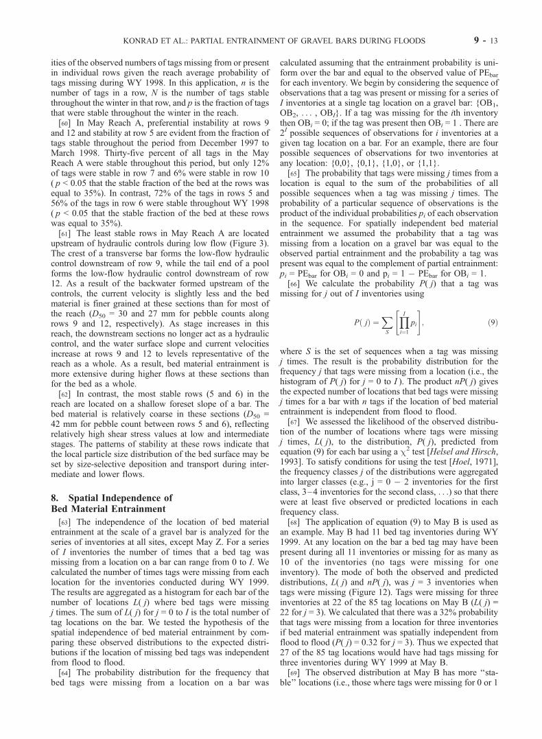
Figure 3. Longitudinal profile and plan view of MayCreek sites.


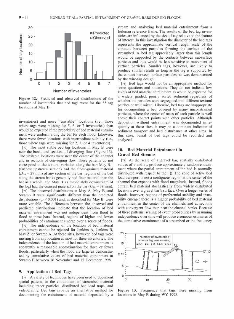
inventories when a tag that appeared to be missing wasactually buried. A buried tag was usually uncovered when anew tag was placed at that location, though occasionally aburied tag was found later in the season. In these cases, thelast recorded instance when the tag was missing was revisedto indicate that the tag had been present. The potential forerrors resulting from the size of the bed tag or drag on theplastic flagging was assessed at two field sites using analternative bed tag design. Plastic flagging attached to a 10-cm-long piece of metal wire bent into a ‘‘U’’ was insertedinto the streambed, like a small croquet wicket, next to eachmetal washer type bed tag at the sites during two periods.The low weight of the wire tags and their small surface areain contact with bed material offered less resistance toentrainment. The two types of tags produced identicalresults (i.e., present or missing) at every location, demon-strating that entrainment of tags did not depend on theweight of the tag relative to the drag on the plastic flagging.We conclude that the weight of metal washers is unlikely toincrease type 1 errors relative to those of the much lighterwire tags. Moreover, type 2 errors are unlikely where bedtags can be placed securely between particles in thestreambed.[21] At each site, the tags were placed at 0.5-m intervals

across the stream channel in rows across the bars. A 30-cmsteel spike was driven into the left stream bank at each row,and the first tag was located 1 m from the spike to ensure

consistent tag locations over time and facilitate finding tagsduring high-flow periods when visibility was poor. Therows had between 9 and 21 tags depending on the width ofthe channel. There were four to eight rows of tags and 45 to103 bed tags at each bar. The rows spanned the channelsfrom bank to bank except at the right end of Jenkins A,row 5, where the bed material was silt and fine organicdebris rather than gravel. Large boulders were locatedat two locations (Swamp A, row 1, tag 9 and Swamp B,row 2, tag 1). Rather than placing tags at these boulders,the boulders were observed to be stable throughout theexperiments.[22] In addition to the five rows of bed tags on the May A

gravel bar (rows 5, 6, 7, 8, and 10), seven rows of bedtags (rows 1, 2, 3, 4, 9, 11, and 12) were placed in thereach around the May A bar to characterize patterns ofbed material entrainment associated with other channelforms. The observations of tags in these seven rows areexcluded from the bar-scale results and are described onlyin section 7 in the context of the spatial variability in partialentrainment.[23] The bed tags were inventoried on 103 occasions

(every 1–4 weeks) at the seven gravel bars from October1997 to December 1999. During the inventories the location(row and tag number) of each missing tag was recorded andthe tag was replaced. The Eulerian experimental designallowed a time series of entrainment to be developed foreach tag location. Generally, bed tags were inventoried aftera single flood peak, with notable exceptions at the SwampCreek sites (three peaks between the bed tag inventories on16 November 1998 and 15 December 1998) and at theJenkins Creek sites (two peak between 7 December 1998and 4 January 1999). At each bar, there was at least oneinventory when no tags had moved since the previousinventory, providing an estimate of the maximum value oft*0 at each site when the bed was stable.

Figure 5. Cross section of bed tag in a streambed.

Figure 4. Longitudinal profiles and plan views of SwampCreek sites.


[24] The peak water stage between inventories wasrecorded at two crest stage gages separated by 10–20 mat the upstream and downstream ends of each gravelbar. The crest stage gages were constructed from steel rods(�1-cm diameter) driven into the streambed near the bank.Hook-and-loop fabric tape (Velcro

1

) was fastened along theexposed rod such that debris suspended in the streamflow(e.g., fine sediment, particulate organic material, and leaves)would collect in the hooks and loops leaving an easilyidentifiable high-water mark.

4. Analytical Methods and Calculations

4.1. Applied Shear Stress

[25] The distribution of t varies over a streambed,typically with low values near stream banks and highvalues near the center of the channel [Chow, 1959, p. 169]as well as local influences from bed material or other flowobstructions [Rouse, 1965]. The total boundary shear stresst0 was used as a central measure of the distribution of theapplied shear stress over a gravel bar. The total boundaryshear stress along a reach with uniform flow is calculatedas

t0 ¼ gwRS ; ð1Þ

where gw is the specific weight of water, R is the hydraulicradius, and S is the calculated energy gradient of thestreamflow along the bar.[26] The peak total boundary shear stress t0 was calcu-

lated with equation (1) for each period between inventories.R was calculated as the wetted cross-sectional area dividedby the wetted perimeter at the surveyed section using themaximum stage recorded between each inventory. Theenergy gradient for each flood at each site was estimatedusing the water surface slope between the two gages(Table 1). The slope calculation assumes that peak stagewas synchronous at each gage. The error in water surfaceslopes is estimated to be at most ±0.001.[27] In uniform flow, t0 is equal and opposite to all of the

pressure and viscous forces on a unit bed area basis thatresist the gravitational acceleration of water as it flowsdownstream. Here t0 includes form drag that acts overregions of flow separation larger than individual particles(around bends and over bars) without contributing to sedi-ment transport and skin friction that acts at the scale ofindividual particles. Skin friction is the only component oft0 that transports sediment [Einstein, 1950; Einstein andBarbarossa, 1952; Smith and McLean, 1977;McLean et al.,1999].[28] Experimental sites were selected in straight reaches

with few obstacles to minimize form drag; however, we didconsider whether t0 provides a reasonable approximation ofskin friction. Local skin friction tg can be estimated fromthe vertical velocity profile in a fully developed boundarylayer (where the vertical velocity profile does not change inthe stream-wise direction) using the Prandtl-Von Karmanlogarithmic velocity distribution [Grass, 1970; Nece andSmith, 1970; Schlichting, 1979; Wilcock, 1996]:

uðzÞ ¼ u*

kln

z

z0

� �; ð2Þ

where u(z) is the velocity at a height z above the bed, K =0.41 is von Karman’s coefficient, z0 is the roughness lengthscale, and u* = (tg/r)

0.5 is the shear velocity associated withskin friction. Values of u* estimated from equation (2)based on measured vertical velocity profiles were comparedto u*0 = (t0/r)

0.5 for cross sections in Jenkins A, May A, andSwamp B.[29] Current velocity was measured at Jenkins A, May B,

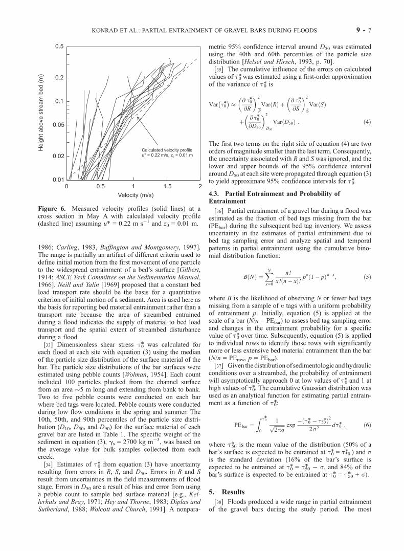
and Swamp B with a Marsh-McBirney current meter at 10–25 positions across the channel at the highest flow when thestreams could be safely waded. At each position, measure-ments were made at 1 cm above the bed and at 5-cmintervals up to the water surface. Shear velocity, u* = K(u1� u2)/ln(z1/z2), was calculated using two velocitymeasurements (u1 and u2) in the near-bed region not morethan 0.2 of flow depth above the bed, where currentvelocities are expected to vary logarithmically [Wiberg andSmith, 1991], notwithstanding the effects of large clastspreventing full development of the turbulent boundarylayer.[30] An example of the velocity profiles and a theoretical

velocity distribution calculated from equation (2) assumingu* = u*0 and z0 = 0.1D84 [Whiting and Dietrich, 1990] isshown for May A on 5 January 1998 (Figure 6). At May A,u* = 0.02 � 0.3 m s�1 for the measured velocity profilescompared to u*0 = 0.22 m s�1 calculated assuming foruniform flow. The value of u*0 is higher than the value ofu* at 90% of the locations across the section. The estimatesof u* based on measured velocity gradients have limitedaccuracy because vertical velocity profiles are not strictlylogarithmic over rough boundaries [Grass, 1971; Wibergand Smith, 1991; Pitlick, 1992]. Furthermore, the velocitiesare mean values measured consecutively over at least a1-min period, rather than simultaneous and instantaneousvelocities, and are likely to have large relative errors for lowvalues near the streambed.[31] For any of the cross sections examined the vertical

velocity gradients spanned a wide range of values withlower vertical velocity gradients near a channel’s banks andsteeper gradients in the center of the channel. Althoughmost of the local values of u* were less than u*0, the valuesof u* in the center of the channel were higher than u*0.Accordingly, we recognize that t0 is only an index of thedistribution of tg and, moreover, t0 is representative of onlythe highest values of tg across a channel.

4.2. Dimensionless Shear Stress

[32] The balance between the applied and resisting shearstresses is represented here by a dimensionless shear stresst*0, which is the ratio of total boundary shear stress to anindex of the unit area buoyant weight of the median of theparticle size distribution:

t0* ¼ t0

gs � gwð ÞD50

; ð3Þ

where gs is the specific weight of the sediment and D50 isthe median of the particle size distribution of the surfacematerial. The reported values of t*0 at the threshold ofmotion (tcr*) for gravel in a turbulent boundary layer span awide range from 0.02 to 0.08 [Fahnstock, 1963; Parker andKlingeman, 1982; Andrews, 1983; Andrews and Erman,


1986; Carling, 1983, Buffington and Montgomery, 1997].The range is partially an artifact of different criteria used todefine initial motion from the first movement of one particleto the widespread entrainment of a bed’s surface [Gilbert,1914; ASCE Task Committee on the Sedimentation Manual,1966]. Neill and Yalin [1969] proposed that a constant bedload transport rate should be the basis for a quantitativecriterion of initial motion of a sediment. Area is used here asthe basis for reporting bed material entrainment rather than atransport rate because the area of streambed entrainedduring a flood indicates the supply of material to bed loadtransport and the spatial extent of streambed disturbanceduring a flood.[33] Dimensionless shear stress t*0 was calculated for

each flood at each site with equation (3) using the medianof the particle size distribution of the surface material of thebar. The particle size distributions of the bar surfaces wereestimated using pebble counts [Wolman, 1954]. Each countincluded 100 particles plucked from the channel surfacefrom an area �5 m long and extending from bank to bank.Two to five pebble counts were conducted on each barwhere bed tags were located. Pebble counts were conductedduring low flow conditions in the spring and summer. The10th, 50th, and 90th percentiles of the particle size distri-bution (D10, D50, and D90) for the surface material of eachgravel bar are listed in Table 1. The specific weight of thesediment in equation (3), gs = 2700 kg m�3, was based onthe average value for bulk samples collected from eachcreek.[34] Estimates of t*0 from equation (3) have uncertainty

resulting from errors in R, S, and D50. Errors in R and Sresult from uncertainties in the field measurements of floodstage. Errors in D50 are a result of bias and error from usinga pebble count to sample bed surface material [e.g., Kel-lerhals and Bray, 1971; Hey and Thorne, 1983; Diplas andSutherland, 1988; Wolcott and Church, 1991]. A nonpara-

metric 95% confidence interval around D50 was estimatedusing the 40th and 60th percentiles of the particle sizedistribution [Helsel and Hirsch, 1993, p. 70].[35] The cumulative influence of the errors on calculated

values of t*0 was estimated using a first-order approximationof the variance of t*0 is

Var t0*� �

� @ t0*

@R

� � 2

R

Var Rð Þ þ @ t0*

@S

� �2

�S

Var Sð Þ

þ @ t0*

@D50

� �2

D50

Var D50ð Þ : ð4Þ

The first two terms on the right side of equation (4) are twoorders of magnitude smaller than the last term. Consequently,the uncertainty associated with R and S was ignored, and thelower and upper bounds of the 95% confidence intervalaroundD50 at each site were propagated through equation (3)to yield approximate 95% confidence intervals for t*0.

4.3. Partial Entrainment and Probability ofEntrainment

[36] Partial entrainment of a gravel bar during a flood wasestimated as the fraction of bed tags missing from the bar(PEbar) during the subsequent bed tag inventory. We assessuncertainty in the estimates of partial entrainment due tobed tag sampling error and analyze spatial and temporalpatterns in partial entrainment using the cumulative bino-mial distribution function:

B Nð Þ ¼XNx¼0

n!

x! n� xð Þ! pn 1� pð Þn�x; ð5Þ

where B is the likelihood of observing N or fewer bed tagsmissing from a sample of n tags with a uniform probabilityof entrainment p. Initially, equation (5) is applied at thescale of a bar (N/n = PEbar) to assess bed tag sampling errorand changes in the entrainment probability for a specificvalue of t*0 over time. Subsequently, equation (5) is appliedto individual rows to identify those rows with significantlymore or less extensive bed material entrainment than the bar(N/n = PErow, p = PEbar).[37] Given the distributionof sedimentologic andhydraulic

conditions over a streambed, the probability of entrainmentwill asymptotically approach 0 at low values of t*0 and 1 athigh values of t*0. The cumulative Gaussian distribution wasused as an analytical function for estimating partial entrain-ment as a function of t*0:

PEbar ¼Z t 0*

0

1ffiffiffiffiffiffiffiffi2ps

p exp� t0*� t50*ð Þ2

2s2dt0* ; ð6Þ

where t*50 is the mean value of the distribution (50% of abar’s surface is expected to be entrained at t*0 = t*50 ) and sis the standard deviation (16% of the bar’s surface isexpected to be entrained at t*0 = t*50 � s, and 84% of thebar’s surface is expected to be entrained at t*0 = t*50 + s).

5. Results

[38] Floods produced a wide range in partial entrainmentof the gravel bars during the study period. The most

Figure 6. Measured velocity profiles (solid lines) at across section in May A with calculated velocity profile(dashed line) assuming u* = 0.22 m s�1 and z0 = 0.01 m.


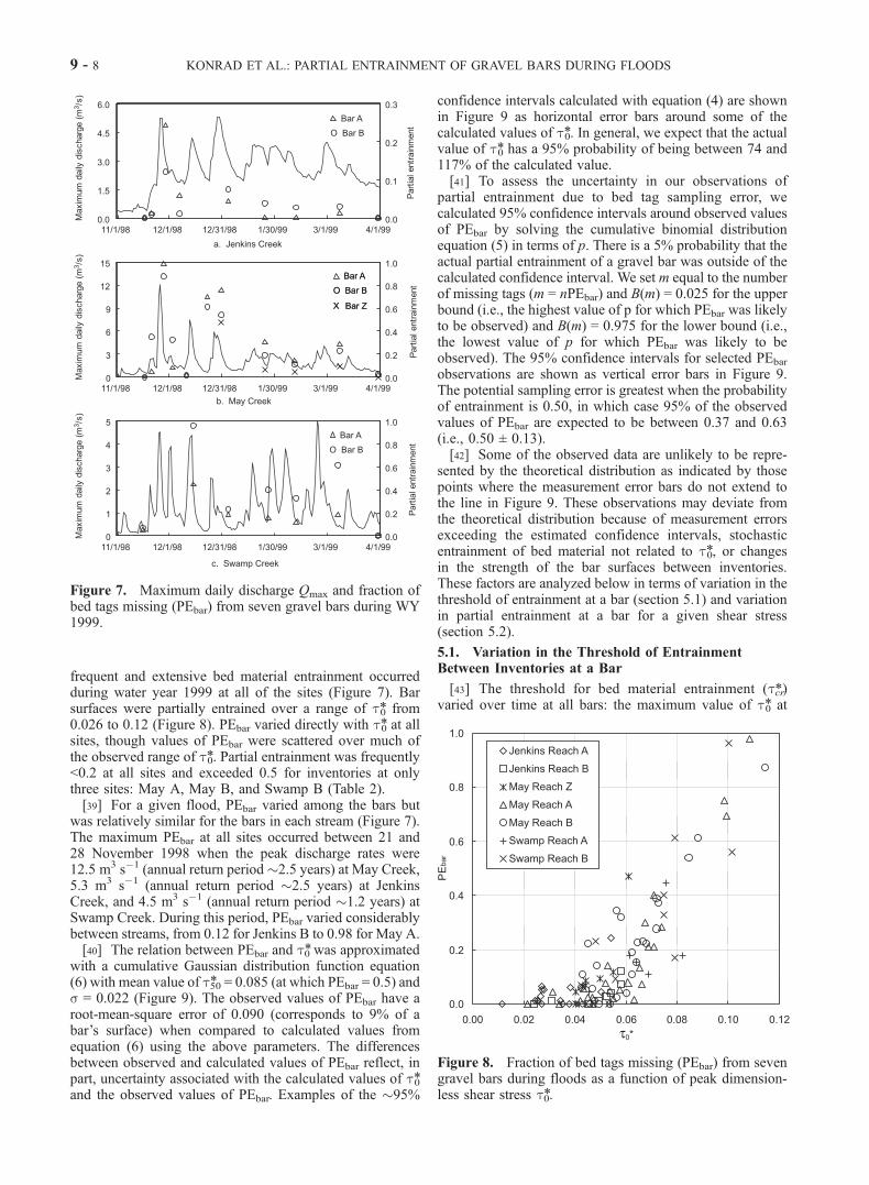
frequent and extensive bed material entrainment occurredduring water year 1999 at all of the sites (Figure 7). Barsurfaces were partially entrained over a range of t*0 from0.026 to 0.12 (Figure 8). PEbar varied directly with t*0 at allsites, though values of PEbar were scattered over much ofthe observed range of t*0. Partial entrainment was frequently<0.2 at all sites and exceeded 0.5 for inventories at onlythree sites: May A, May B, and Swamp B (Table 2).[39] For a given flood, PEbar varied among the bars but

was relatively similar for the bars in each stream (Figure 7).The maximum PEbar at all sites occurred between 21 and28 November 1998 when the peak discharge rates were12.5 m3 s�1 (annual return period�2.5 years) at May Creek,5.3 m3 s�1 (annual return period �2.5 years) at JenkinsCreek, and 4.5 m3 s�1 (annual return period �1.2 years) atSwamp Creek. During this period, PEbar varied considerablybetween streams, from 0.12 for Jenkins B to 0.98 for May A.[40] The relation between PEbar and t*0 was approximated

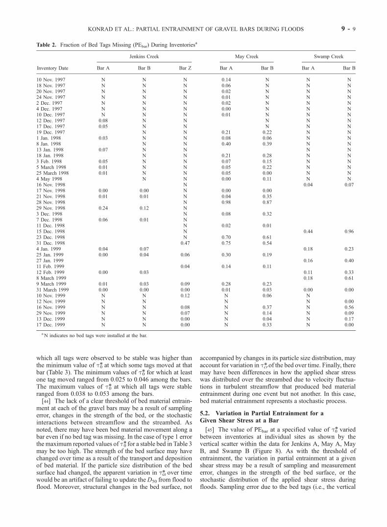
with a cumulative Gaussian distribution function equation(6) with mean value of t*50 = 0.085 (at which PEbar = 0.5) ands = 0.022 (Figure 9). The observed values of PEbar have aroot-mean-square error of 0.090 (corresponds to 9% of abar’s surface) when compared to calculated values fromequation (6) using the above parameters. The differencesbetween observed and calculated values of PEbar reflect, inpart, uncertainty associated with the calculated values of t*0and the observed values of PEbar. Examples of the �95%

confidence intervals calculated with equation (4) are shownin Figure 9 as horizontal error bars around some of thecalculated values of t*0. In general, we expect that the actualvalue of t*0 has a 95% probability of being between 74 and117% of the calculated value.[41] To assess the uncertainty in our observations of

partial entrainment due to bed tag sampling error, wecalculated 95% confidence intervals around observed valuesof PEbar by solving the cumulative binomial distributionequation (5) in terms of p. There is a 5% probability that theactual partial entrainment of a gravel bar was outside of thecalculated confidence interval. We set m equal to the numberof missing tags (m = nPEbar) and B(m) = 0.025 for the upperbound (i.e., the highest value of p for which PEbar was likelyto be observed) and B(m) = 0.975 for the lower bound (i.e.,the lowest value of p for which PEbar was likely to beobserved). The 95% confidence intervals for selected PEbar

observations are shown as vertical error bars in Figure 9.The potential sampling error is greatest when the probabilityof entrainment is 0.50, in which case 95% of the observedvalues of PEbar are expected to be between 0.37 and 0.63(i.e., 0.50 ± 0.13).[42] Some of the observed data are unlikely to be repre-

sented by the theoretical distribution as indicated by thosepoints where the measurement error bars do not extend tothe line in Figure 9. These observations may deviate fromthe theoretical distribution because of measurement errorsexceeding the estimated confidence intervals, stochasticentrainment of bed material not related to t*0, or changesin the strength of the bar surfaces between inventories.These factors are analyzed below in terms of variation in thethreshold of entrainment at a bar (section 5.1) and variationin partial entrainment at a bar for a given shear stress(section 5.2).

5.1. Variation in the Threshold of EntrainmentBetween Inventories at a Bar

[43] The threshold for bed material entrainment (tcr*)varied over time at all bars: the maximum value of t*0 at

Figure 7. Maximum daily discharge Qmax and fraction ofbed tags missing (PEbar) from seven gravel bars during WY1999.

Figure 8. Fraction of bed tags missing (PEbar) from sevengravel bars during floods as a function of peak dimension-less shear stress t*0.


which all tags were observed to be stable was higher thanthe minimum value of t*0 at which some tags moved at thatbar (Table 3). The minimum values of t*0 for which at leastone tag moved ranged from 0.025 to 0.046 among the bars.The maximum values of t*0 at which all tags were stableranged from 0.038 to 0.053 among the bars.[44] The lack of a clear threshold of bed material entrain-

ment at each of the gravel bars may be a result of samplingerror, changes in the strength of the bed, or the stochasticinteractions between streamflow and the streambed. Asnoted, there may have been bed material movement along abar even if no bed tag was missing. In the case of type 1 errorthe maximum reported values of t*0 for a stable bed in Table 3may be too high. The strength of the bed surface may havechanged over time as a result of the transport and depositionof bed material. If the particle size distribution of the bedsurface had changed, the apparent variation in tcr* over timewould be an artifact of failing to update theD50 from flood toflood. Moreover, structural changes in the bed surface, not

accompanied by changes in its particle size distribution, mayaccount for variation in tcr* of the bed over time. Finally, theremay have been differences in how the applied shear stresswas distributed over the streambed due to velocity fluctua-tions in turbulent streamflow that produced bed materialentrainment during one event but not another. In this case,bed material entrainment represents a stochastic process.

5.2. Variation in Partial Entrainment for aGiven Shear Stress at a Bar

[45] The value of PEbar at a specified value of t*0 variedbetween inventories at individual sites as shown by thevertical scatter within the data for Jenkins A, May A, MayB, and Swamp B (Figure 8). As with the threshold ofentrainment, the variation in partial entrainment at a givenshear stress may be a result of sampling and measurementerror, changes in the strength of the bed surface, or thestochastic distribution of the applied shear stress duringfloods. Sampling error due to the bed tags (i.e., the vertical

Table 2. Fraction of Bed Tags Missing (PEbar) During Inventoriesa

Inventory Date

Jenkins Creek May Creek Swamp Creek

Bar A Bar B Bar Z Bar A Bar B Bar A Bar B

10 Nov. 1997 N N N 0.14 N N N18 Nov. 1997 N N N 0.06 N N N20 Nov. 1997 N N N 0.02 N N N24 Nov. 1997 N N N 0.01 N N N2 Dec. 1997 N N N 0.02 N N N4 Dec. 1997 N N N 0.00 N N N10 Dec. 1997 N N N 0.01 N N N12 Dec. 1997 0.08 N N N N N17 Dec. 1997 0.05 N N N N N19 Dec. 1997 N N 0.21 0.22 N N1 Jan. 1998 0.03 N N 0.08 0.06 N N8 Jan. 1998 N N 0.40 0.39 N N13 Jan. 1998 0.07 N N N N18 Jan. 1998 N N 0.21 0.28 N N3 Feb. 1998 0.05 N N 0.07 0.15 N N5 March 1998 0.01 N N 0.05 0.22 N N25 March 1998 0.01 N N 0.05 0.00 N N4 May 1998 N N 0.00 0.11 N N16 Nov. 1998 N 0.04 0.0717 Nov. 1998 0.00 0.00 N 0.00 0.0021 Nov. 1998 0.01 0.01 N 0.04 0.3528 Nov. 1998 N 0.98 0.8729 Nov. 1998 0.24 0.12 N3 Dec. 1998 N 0.08 0.327 Dec. 1998 0.06 0.01 N11 Dec. 1998 N 0.02 0.0115 Dec. 1998 N 0.44 0.9623 Dec. 1998 N 0.70 0.6131 Dec. 1998 0.47 0.75 0.544 Jan. 1999 0.04 0.07 0.18 0.2325 Jan. 1999 0.00 0.04 0.06 0.30 0.1927 Jan. 1999 0.16 0.4011 Feb. 1999 0.04 0.14 0.1112 Feb. 1999 0.00 0.03 0.11 0.338 March 1999 0.18 0.619 March 1999 0.01 0.03 0.09 0.28 0.2331 March 1999 0.00 0.00 0.00 0.01 0.03 0.00 0.0010 Nov. 1999 N N 0.12 N 0.06 N12 Nov. 1999 N N N N 0.0016 Nov. 1999 N N 0.08 N 0.37 N 0.5629 Nov. 1999 N N 0.07 N 0.14 N 0.0913 Dec. 1999 N N 0.00 N 0.04 N 0.1717 Dec. 1999 N N 0.00 N 0.33 N 0.00

aN indicates no bed tags were installed at the bar.


error bars in Figure 9) might account for some of theobserved variation in PEbar at a site for a given value oft*0, but it is unlikely to account for all of the variation. Heret*0 has a margin of error related to the hydraulic calcula-tions, the estimate of D50, and the approximation of tg byt0. These errors are likely to introduce a uniform bias forfloods of similar magnitudes at a site, so they are unlikely toaccount for variation over time in the relation between PEbar

and t*0 at a site.[46] Variation in PEbar for a given value of t*0 also may

represent actual differences in the spatial extent of bedmaterial entrainment that could arise because of variableflood durations or changes in bed surface strength duringfloods. First, partial entrainment may vary with the durationof a flood, which is not represented by t*0. For example,inventories conducted after multiple flood peaks indicatehigher values of PEbar relative to t*0 than inventoriesconducted after a single flood peak. The hydrograph forSwamp Creek (Figure 7) shows three distinct peaks indischarge rate for the period prior to the 15 December1998 inventory, whereas there was only one peak for theperiod prior to the 16 November 1999 inventory. As aresult, the inventory on 15 December 1998 had a largerfraction of tags missing (PEbar = 0.96) than the 16 Novem-ber 1999 inventory (PEbar = 0.56), even though t*0 was 0.10for both inventories (Figure 7). The value of PEbar for aninventory after F flood peaks can be calculated assumingindependent entrainment of bed tags from flood to flood as

PEbar ¼ 1�YFf¼ 1

1� PEbar f

� �; ð7Þ

where 1 � PEbar f is the fraction of the bar that was stable inthe f th flood. In the Swamp Creek example the expected

value of PEbar for the 15 December 1998 inventory wascalculated using equation (7) by setting PEbarj equal to0.75, the expected value of PEbar for a single flood when t*0= 0.10 based on equation (3), for each of the three peaks(F = 3). The cumulative entrainment predicted fromequation (6) is 0.98 compared to an observed value of 0.96.[47] In contrast, PEbar at the Jenkins Creek sites for two

flood peaks between 7 December 1998 and 4 January 1999is lower than PEbar for a previous flood in November 1998of similar magnitude (Figure 7). We suggest that the differ-ence between the streams may be related to the magnitudeof the floods. In Swamp Creek the floods were capable ofentraining over half of the bed surface, whereas the floodsin Jenkins Creek were capable of entraining a quarter of thebed surface at most. Large floods may rearrange particles onthe bed surface, equivalent to reshuffling a deck of cards,and maintain the independent selection of grains from thesurface. Small floods, however, remove small and uncon-strained particles such that the probability of entrainment isnot independent from event to event.[48] The potential influence of flow duration on partial

entrainment was examined for May B. As an alternative toshear stress, stream power has been used to analyze sedi-ment transport rates [Bagnold, 1977] and can be integratedover time to assess the work done by a river movingsediment. An index of the work per unit of streambed areafor each inventory was calculated in discrete form asproduct of excess unit stream power (w � wc) and time(900 s) summed over the period (t) since the previousinventory:

� ¼ 900Xt

ðw� wcÞ3=2; ð8Þ

where w = gwQS/w, w is channel width, wc = 9.8 W m�2

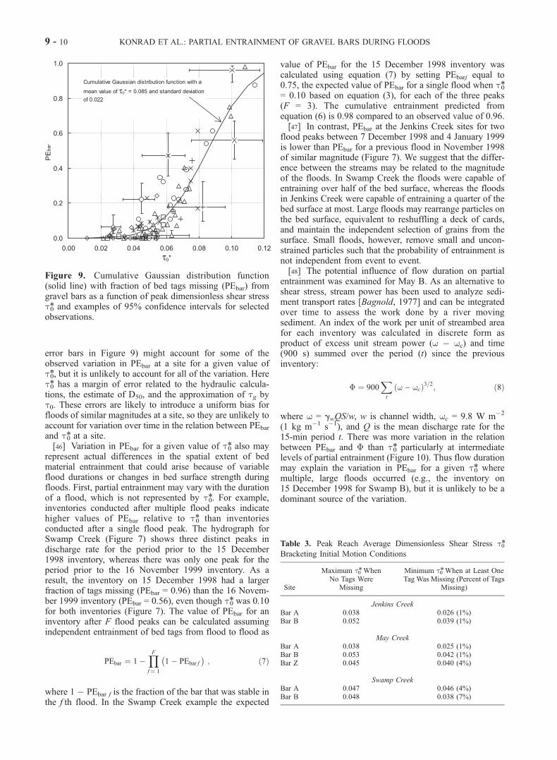
(1 kg m�1 s�1), and Q is the mean discharge rate for the15-min period t. There was more variation in the relationbetween PEbar and � than t*0 particularly at intermediatelevels of partial entrainment (Figure 10). Thus flow durationmay explain the variation in PEbar for a given t*0 wheremultiple, large floods occurred (e.g., the inventory on15 December 1998 for Swamp B), but it is unlikely to be adominant source of the variation.

Table 3. Peak Reach Average Dimensionless Shear Stress t*0Bracketing Initial Motion Conditions

Site

Maximum t*0 WhenNo Tags Were

Missing

Minimum t*0 When at Least OneTag Was Missing (Percent of Tags

Missing)

Jenkins CreekBar A 0.038 0.026 (1%)Bar B 0.052 0.039 (1%)

May CreekBar A 0.038 0.025 (1%)Bar B 0.053 0.042 (1%)Bar Z 0.045 0.040 (4%)

Swamp CreekBar A 0.047 0.046 (4%)Bar B 0.048 0.038 (7%)

Figure 9. Cumulative Gaussian distribution function(solid line) with fraction of bed tags missing (PEbar) fromgravel bars as a function of peak dimensionless shear stresst*0 and examples of 95% confidence intervals for selectedobservations.


[49] Instead, streamflow is likely to modify the structureof the bed surface or its particle size distribution betweeninventories, resulting in variation in PEbar for a given valueof t*0 over time. Flow-mediated changes in the strength ofthe bed surface were analyzed for pairs of inventories at asite when t*0 differed by no more than 0.005. Values ofPEbar for the pairs were tested to determine if they werelikely to represent two outcomes of floods with the sameprobability of entrainment. For each pair the cumulativebinomial distribution function equation (5) was appliediteratively to find the entrainment probability p at whichthe likelihood, B(N ), of the two observed values of PEbar

were equal. (Here p is approximately equal to the mean ofthe observed values of PEbar for the pair of inventories.)When the likelihood of observing the two values of PEbar

was <5%, given p, the two inventories were considered tobe significantly different.

[50] There were six pairs of inventories where t*0 wasequal for the two inventories in the pair but the values of PEwere significantly different. These inventories occurred atfour gravel bars (Jenkins A, May A, May B, and Swamp B)(Table 4). In five of the pairs, PEbar for the first inventorywas greater than PEbar for the second inventory, whichrepresents an increase in bar strength over time. The greatestincrease in bar strength occurred at Swamp B where PEbar

decreased from 0.61 to 0.17 for two floods when t*0 was0.082. Other inventories show a pattern of increasing bedstability over time, though the differences in PEbar were notstatistically significant.[51] Only one pair of inventories showed a significant

increase in the extent of bed material entrainment over a pairof floods with similar magnitudes. At May B, PEbar was0.06 when t*0 was 0.046 for a flood on 1 January 1998;PEbar was 0.22 when t*0 was 0.044 for a flood on 5 March1998. Between January and March 1998, there were threeintervening floods, with values of PEbar ranging from 0.15to 0.39, that may have modified the structure or texture ofthe bed surface at May B.

6. Influence of Past Floods onPartial Entrainment DuringIntermediate Magnitude Floods

[52] Flow-mediated changes in the strength of bar surfaceswere further analyzed in terms of the influence of past floodson partial entrainment for all floods when t*0 was 0.055 to0.070 (Table 5). We hypothesized that after large floods, thebed surface would be relatively weaker (e.g., because anarmored surface was breached but not reestablished) thanafter an intermediate flood. Under this hypothesis we positthat recessional flows from a single, large flood would not besufficient to reestablish an armor layer. As a result, partialentrainment for a flood when 0.055 < t*0 < 0.070 would behigher when the previous flood was large than partial entrain-ment for other floods when 0.055 < t*0 < 0.070. Furthermore,intermediate-magnitude floods would strengthen the bedsurface, so that partial entrainment for a flood when 0.055< t*0 < 0.070 would be lower than expected when theprevious flood was of intermediate magnitude.[53] The analysis compared values of PE for intermediate

magnitude floods to the strength of the previous flood withinthat season. We selected only inventories when t*0 rangedfrom 0.055 to 0.070 because the variation of PEbar was large(from 0 to 0.48) among these inventories but not stronglyrelated to the variation in t*0 (Figure 8). The inventories were

Table 4. Significantly Different Values of Partial Entrainment (PEbar) at a Site for Floods of Similar Magnitude

Site

First Inventory Second Inventory Probability of Entrainmentfor Equal Likelihood of

Observed Values of PEbarsDate t0* PEbar Date t0* PEbar

Jenkins Aa 29 Nov. 1998 0.056 0.24 4 Jan. 1999 0.052 0.04 0.13May Aa 8 Jan. 1998 0.073 0.4 18 Jan. 1998 0.073 0.21 0.30Swamp Ba 4 Jan. 1999 0.045 0.23 12 Nov. 1999 0.047 0.00 0.10Swamp Ba 8 March 1999 0.082 0.61 13 Dec. 1999 0.082 0.17 0.38May Aa 25 Jan. 1999 0.070 0.30 11 Feb. 1999 0.068 0.14 0.22May Bb 1 Jan. 1998 0.046 0.06 5 March 1998 0.044 0.22 0.14

a Increase in bed stability over time.bDecrease in bed stability over time.

Figure 10. Relations of partial entrainment (PE) to unitarea work index and dimensionless shear stress at May B.Unit area work index is �(w � wcr)

3/2, where w is unit areastream power and wcr = 9.8 W m�2.


divided into four groups on the basis of the value of thepeak dimensionless shear stress for the previous inventory(tp*). Inventories when 0.026 < tp* < 0.054 were in groupA. Inventories when 0.060 < tp* < 0.064 were in group B.Inventories when 0.065 < tp* < 0.074 were in group C.Inventories when 0.084 < tp* < 0.115 were in group D.[54] The mean value of PEbar for all inventories when

0.055 < t*0 < 0.070 was 0.15. The mean value of PEbar forgroups A and B was 0.14, for group C was 0.08, and forgroup D was 0.20. Only groups C (previous flood had anintermediate magnitude) and D (previous flood with a highmagnitude) were significantly different ( p < 0.05 based on aone-tailed Student’s t distribution). The results demonstratehigher bed strength (lower PEbar) after intermediate-magni-tude flows (0.065 < t*0 < 0.074) and lower bed strength(higher PEbar) after high flows (t*0 > 0.84).[55] Changes in the strength of the streambed at the sites

were not associated with any significant changes (<5 mm)in the median diameter of bed material from summer tosummer. There may have been transient changes in bedmaterial texture between storms [e.g., Gomez, 1983a] thatwere not evident from the results of pebble counts con-ducted during periods of lower flow. Bed strength also mayhave increased as particles were moved into more stablepositions without detectable changes in the particle sizedistributions over time.

7. Spatial Uniformity ofBed Material Entrainment

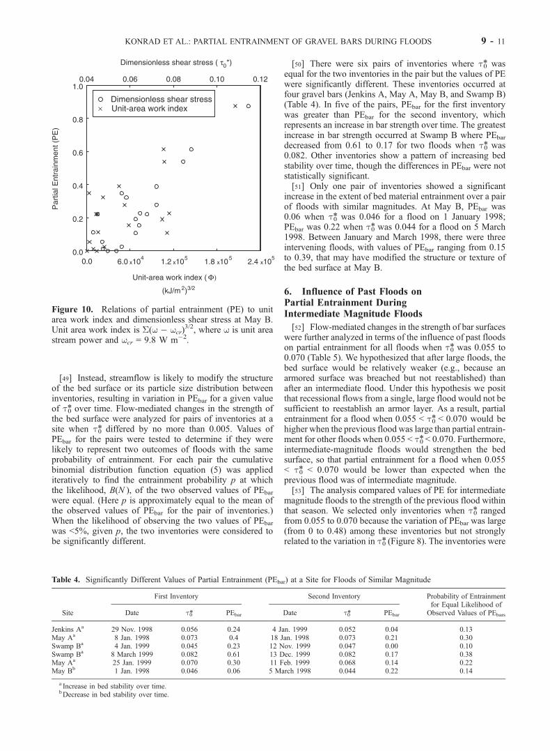
[56] The hypothesis that the probability of entrainment isuniform over a gravel bar during a flood was tested bycomparing the fraction of bed tags missing for a bar (PEbar)to the fraction of tags missing from each row in the bar(PErow). There were 372 PEbar, PErow pairs for which at leastone tag was missing from the gravel bar. The pairs areplotted in Figure 11. For each pair the probability ofobserving PErow given PEbar was determined using thecumulative binomial distribution equation (5), where p isequal to PEbar, n is the number of tags in the row, and N isthe number of tags missing from that row (i.e., N/n = PErow).[57] Most observations of PErow (341 or 92%) were

within the 95% confidence interval around PEbar (circlesin Figure 11). However, PErow differed significantly fromPEbar for 31 instances (crosses in Figure 11). There were10 instances when the fraction of tags entrained at a rowwas significantly less than fraction entrained at the bar(PErow was below the confidence intervals for PEbar) and21 instances when the fraction of tags entrained at a rowwas significantly greater than the fraction entrained at thebar. The anomalously low and high values of PErow were

distributed among 16 rows at all of the sites, except SwampA, and occurred during periods with both high and lowlevels of partial entrainment.[58] At six rows, PErow was significantly different than

PEbar for more than one inventory. Values of PErow wereless than PEbar at two of the rows (May A.5 and SwampB.1). These relatively stable rows were located in regions ofdivergent flow where the channel widened slightly down-stream. Values of PErow were greater than PEbar at four ofthe rows (May A.7, A.10, and B.3 and Swamp B.3). Theseless stable rows were in regions of converging flow (MayA.7 and B.3) and along the foreset slope of a bar (May A.10and Swamp B.3).[59] The uniform probability hypothesis was also tested

for a reach spanning the bar at May A and including portionsof a downstream pool (Figure 3). As with the analysis of thebars, preferential entrainment and stability of rows in MayReach A was evaluated using the cumulative binomialdistribution function equation (5) to calculate the probabil-

Table 5. Partial Entrainment for Inventories When 0.055 < t*0 < 0.070 Illustrating the Influence of Previous Floods on Bed Stability

Group A Group B Group C Group D

Dimensionless shear stress of previous flood tp*Mean of group 0.043 0.062 0.07 0.10Range of group 0.026–0.054 0.060–0.064 0.065–0.074 0.084–0.115

Number of inventories 8 6 5 5Mean dimensionless shear stress for inventories in group t*0 0.060 0.064 0.063 0.061Partial entrainment, PEbar 0.143 0.142 0.080 0.196

Figure 11. Comparison of partial entrainment at rows(PErow) and bars (PEbar), where crosses indicate that theprobability of entrainment at a row was unlikely ( p < 0.05)to be equal to the probability of entrainment for thesurrounding bar.


ities of the observed numbers of tags missing from or presentin individual rows given the reach average probability oftags missing during WY 1998. In this application, n is thenumber of tags in a row, N is the number of tags stablethroughout the winter in that row, and p is the fraction of tagsthat were stable throughout the winter in the reach.[60] In May Reach A, preferential instability at rows 9

and 12 and stability at row 5 are evident from the fraction oftags stable throughout the period from December 1997 toMarch 1998. Thirty-five percent of all tags in the MayReach A were stable throughout this period, but only 12%of tags were stable in row 7 and 6% were stable in row 10( p < 0.05 that the stable fraction of the bed at the rows wasequal to 35%). In contrast, 72% of the tags in rows 5 and56% of the tags in row 6 were stable throughout WY 1998( p < 0.05 that the stable fraction of the bed at these rowswas equal to 35%).[61] The least stable rows in May Reach A are located

upstream of hydraulic controls during low flow (Figure 3).The crest of a transverse bar forms the low-flow hydrauliccontrol downstream of row 9, while the tail end of a poolforms the low-flow hydraulic control downstream of row12. As a result of the backwater formed upstream of thecontrols, the current velocity is slightly less and the bedmaterial is finer grained at these sections than for most ofthe reach (D50 = 30 and 27 mm for pebble counts alongrows 9 and 12, respectively). As stage increases in thisreach, the downstream sections no longer act as a hydrauliccontrol, and the water surface slope and current velocitiesincrease at rows 9 and 12 to levels representative of thereach as a whole. As a result, bed material entrainment ismore extensive during higher flows at these sections thanfor the bed as a whole.[62] In contrast, the most stable rows (5 and 6) in the

reach are located on a shallow foreset slope of a bar. Thebed material is relatively coarse in these sections (D50 =42 mm for pebble count between rows 5 and 6), reflectingrelatively high shear stress values at low and intermediatestages. The patterns of stability at these rows indicate thatthe local particle size distribution of the bed surface may beset by size-selective deposition and transport during inter-mediate and lower flows.

8. Spatial Independence ofBed Material Entrainment

[63] The independence of the location of bed materialentrainment at the scale of a gravel bar is analyzed for theseries of inventories at all sites, except May Z. For a seriesof I inventories the number of times that a bed tag wasmissing from a location on a bar can range from 0 to I. Wecalculated the number of times tags were missing from eachlocation for the inventories conducted during WY 1999.The results are aggregated as a histogram for each bar of thenumber of locations L( j) where bed tags were missingj times. The sum of L( j) for j = 0 to I is the total number oftag locations on the bar. We tested the hypothesis of thespatial independence of bed material entrainment by com-paring these observed distributions to the expected distri-butions if the location of missing bed tags was independentfrom flood to flood.[64] The probability distribution for the frequency that

bed tags were missing from a location on a bar was

calculated assuming that the entrainment probability is uni-form over the bar and equal to the observed value of PEbar

for each inventory. We begin by considering the sequence ofobservations that a tag was present or missing for a series ofI inventories at a single tag location on a gravel bar: {OB1,OB2, . . . , OBI}. If a tag was missing for the ith inventorythen OBi = 0; if the tag was present then OBi = 1 . There are2I possible sequences of observations for i inventories at agiven tag location on a bar. For an example, there are fourpossible sequences of observations for two inventories atany location: {0,0}, {0,1}, {1,0}, or {1,1}.[65] The probability that tags were missing j times from a

location is equal to the sum of the probabilities of allpossible sequences when a tag was missing j times. Theprobability of a particular sequence of observations is theproduct of the individual probabilities pi of each observationin the sequence. For spatially independent bed materialentrainment we assumed the probability that a tag wasmissing from a location on a gravel bar was equal to theobserved partial entrainment and the probability a tag waspresent was equal to the complement of partial entrainment:pi = PEbar for OBi = 0 and pi = 1 � PEbar for OBi = 1.[66] We calculate the probability P( j) that a tag was

missing for j out of I inventories using

Pð jÞ ¼XS

YIi¼1

pi

" #; ð9Þ

where S is the set of sequences when a tag was missingj times. The result is the probability distribution for thefrequency j that tags were missing from a location (i.e., thehistogram of P( j) for j = 0 to I ). The product nP( j) givesthe expected number of locations that bed tags were missingj times for a bar with n tags if the location of bed materialentrainment is independent from flood to flood.[67] We assessed the likelihood of the observed distribu-

tion of the number of locations where tags were missingj times, L( j), to the distribution, P( j), predicted fromequation (9) for each bar using a c2 test [Helsel and Hirsch,1993]. To satisfy conditions for using the test [Hoel, 1971],the frequency classes j of the distributions were aggregatedinto larger classes (e.g., j = 0 � 2 inventories for the firstclass, 3–4 inventories for the second class, . . .) so that therewere at least five observed or predicted locations in eachfrequency class.[68] The application of equation (9) to May B is used as

an example. May B had 11 bed tag inventories during WY1999. At any location on the bar a bed tag may have beenpresent during all 11 inventories or missing for as many as10 of the inventories (no tags were missing for oneinventory). The mode of both the observed and predicteddistributions, L( j) and nP( j), was j = 3 inventories whentags were missing (Figure 12). Tags were missing for threeinventories at 22 of the 85 tag locations on May B (L( j) =22 for j = 3). We calculated that there was a 32% probabilitythat tags were missing from a location for three inventoriesif bed material entrainment was spatially independent fromflood to flood (P( j) = 0.32 for j = 3). Thus we expected that27 of the 85 tag locations would have had tags missing forthree inventories during WY 1999 at May B.[69] The observed distribution at May B has more ‘‘sta-

ble’’ locations (i.e., those where tags were missing for 0 or 1


inventories) and more ‘‘unstable’’ locations (i.e., thosewhere tags were missing for 5, 6, or 7 inventories) thanwould be expected if the probability of bed material entrain-ment were uniform along the bar for each flood. Likewise,there were fewer locations with intermediate stability (i.e.,those where tags were missing for 2, 3, or 4 inventories).[70] The most stable bed tag locations in May B were

near the banks and sections of diverging flow (Figure 13).The unstable locations were near the center of the channeland in sections of converging flow. These patterns do notcorrespond to the textural variation along the bar: May B.1(farthest upstream section) had the finest-grained material(D50 = 27 mm) of any section of the bar; regions of the bedalong the stream banks generally had finer material than thebar as a whole, and May B.3 (immediately downstream ofthe log) had the coarsest material on the bar (D50 = 38 mm).[71] The observed distributions at May A, May B, and

Swamp B were significantly different than the predicteddistributions ( p < 0.001) and, as described for May B, weremore variable. The differences between the observed andpredicted distributions indicate that the location of bedmaterial entrainment was not independent from flood toflood at these bars. Instead, regions of higher and lowerprobabilities of entrainment emerge over a series of floods.[72] The independence of the location of bed material

entrainment cannot be rejected for Jenkins A, Jenkins B,May Z, or Swamp A. At these sites, however, bed tags weremissing from any location at most for three inventories. Theindependence of the location of bed material entrainment isapparently a reasonable approximation for three or fewerfloods, particularly when the flood are large as demonstra-ted by cumulative extent of bed material entrainment atSwamp B between 16 November and 15 December 1998.

9. Application of Bed Tags

[73] A variety of techniques have been used to documentspatial patterns in the entrainment of streambed materialincluding tracer particles, distributed bed load traps, andvideography. Bed tags provide an alternative method fordocumenting the entrainment of material deposited by a

stream and analyzing bed material entrainment from aEulerian reference frame. The results of the bed tag inven-tories are influenced by the size of tag relative to the featureof interest. In this investigation the diameter of the bed tagsrepresents the approximate vertical length scale of thecontacts between particles forming the surface of thestreambed. A bed tag appreciably larger than this lengthwould be supported by the contacts between subsurfaceparticles and thus would be less sensitive to movement ofsurface particles. Smaller tags, however, are likely toproduce similar results as long as the tag is supported bythe contact between surface particles, as was demonstratedby the wire-tag design.[74] Bed tags would not be an appropriate method for

some questions and situations. They do not indicate lowlevels of bed material entrainment as would be expected fora widely graded, poorly sorted sediment regardless ofwhether the particles were segregated into different texturalpatches or well mixed. Likewise, bed tags are inappropriatefor documenting a bed covered by many unconstrainedparticles, where the center of mass of each particle is wellabove their contact points with other particles. Althoughdeposition without entrainment was documented infre-quently at these sites, it may be a dominant indicator ofsediment transport and bed disturbance at other sites. Inthis case, burial of bed tags could be recorded andanalyzed.

10. Bed Material Entrainment inGravel Bed Streams

[75] At the scale of a gravel bar, spatially distributedvalues of t and tcr produce approximately random entrain-ment where the partial entrainment of the bed is normallydistributed with respect to the t*0. The zone of active bedload transport is not a contiguous region at the center of thechannel that expands with flood magnitude. Instead, floodsentrain bed material stochastically from widely distributedlocations over a gravel bar’s surface. Over a longer series offloods, however, regions of preferential stability and insta-bility emerge: there is a higher probability of bed materialentrainment in the center of the channels and at sectionswith convergent flow than near the channel banks. Becauseof these patterns, scaling of event probabilities by assumingindependence over time will produce erroneous estimates ofthe cumulative entrainment of a streambed or the frequency

Figure 12. Predicted and observed distributions of thenumber of inventories that bed tags were for the 85 taglocations at May B.

Figure 13. Frequency that tags were missing fromlocations in May B during WY 1998.


of entrainment at a location over multiple flood events. Inthese cases, additional information about flow-mediatedchanges in the strength of the bed and the spatial distribu-tions of t and tcr are needed to assess sediment supply forbed load transport and streambed disturbance over periodsgreater than individual floods.[76] Intermediate-magnitude floods appear to strengthen

bar surfaces, perhaps by removing small and unconstrainedparticles from the streambed, rearranging particles into morestable structures, and depositing large particles. As a con-sequence, the probability of bed material entrainment is notindependent from event to event but, instead, declines overa series of small to intermediate events. Streamflow is likelyto produce this effect only in gravel bed streams where thesediment supply is limited.[77] Floods begin to weaken the bed surface when they

entrain �50% of a bar’s surface. Under such a condition,bed material is transported indiscriminately with respect toparticle size such that the bed surface is unlikely to armor orotherwise form stable structures [Little and Mayer, 1976;Garde et al., 1977; Gomez, 1983a, 1983b; Shen and Lu,1983; Kuhnle and Southard, 1988; Hassan and Reid, 1990;Chin et al., 1992]. In contrast to small and intermediatefloods, large floods maintain the spatial independence ofbed material entrainment by transporting particles withoutregard to their size and rearranging much of the bed surface.[78] The influence of flow duration on partial entrainment

remains to be tested thoroughly as the duration of floodscould not be controlled in these unregulated streams. Wil-cock and McArdell [1997] observed that the active portionof a bed increases over time reach a constant at a timescaledependent on the transport rate and bed length. Theysuggested that the timescale may be longer than the durationof high flows in many streams. In this case, PEbar would beinfluenced by flow duration. Indeed, cumulative values ofPEbar increased over multiple flood events in some cases.However, the decline in PEbar over time and the spatialdependence of bed material entrainment indicates that theactive portion of the bed may attain an equilibrium valueover a period of multiple floods in streams until a largeevent reorders particles. Partial entrainment does not varystrongly with stream power integrated over time. In thisway, patterns of bed material entrainment are unlike sedi-ment transport rates, which can be maintained by a smallpopulation of active particles and thus are likely to related tostream power.

11. Conclusions

[79] Most floods in gravel bed streams entrain only aportion of the material forming the streambed surface. Thepartial entrainment of streambed provides an estimate of theprobability of entrainment. In this investigation of sevengravel bars in three streams the partial entrainment of gravelbars had a Gaussian distribution with respect to the peak t*0of a flood. The distribution had a mean value of t*0 = 0.085(at which 50% of a bar’s surface is expected to beentrained), a standard deviation of 0.022, and a root-mean-square error of 9% of a bar’s surface compared toobserved partial entrainment. Partial entrainment was notconsistently related to the return period of a flood among thestreams: PEbar for a 2.5-year event varied from <10% inJenkins Creek to >90% in May Creek.

[80] The simple stochastic relation between t0* and partialentrainment provides a means for calculating the extent ofdisturbance during a flood of a gravel streambed comprisinga single particle size distribution (either unimodal or bimo-dal) and uniform flow conditions. The relation can alsoserve as an event-scale probability of entrainment forestimating the sediment supplied from a streambed to bedload transport.[81] The variation in partial entrainment of a gravel bar

at a given value of t*0 may result from the low precision ofPEbar estimates, the failure of t*0 to account for thecumulative entrainment of the streambed over a periodof time (particularly for multiple floods), or flow-mediatedchanges in the strength of the bed surface. The transitionbetween floods that strengthened the bed surface from thelarger floods that weakened the bed occurred at a value oft*0 of �0.08, when �50% of a bar’s surface would beentrained.[82] The probability of bed material was approximately

uniform over a gravel bar during a flood, provided the barhad uniform sedimentologic and hydraulic conditions. Bedmaterial entrainment is only approximately independentfrom flood to flood, particularly during and after largefloods that entrain 50% or more of a bar. In contrast, theprobability of entrainment declined for a series of consec-utive small and intermediate magnitude floods. Bed materialnear the center of a channel and in laterally or verticallyconvergent sections was likely to be entrained more fre-quently than the material near the channel banks and insections of divergent streamflow over the course of a wetseason. The deviations from uniform and independent bedmaterial entrainment prevent simple scaling of event prob-abilities over periods spanning multiple floods to estimatethe supply of material for bed load transport or the cumu-lative extent of streambed disturbance.

[83] Acknowledgments. This work was supported in part by the U.S.Environmental Protection Agency, Water and Watersheds Program underagreement R82-5484-010. Suggestions by Ned Andrews, John Pitlick, andtwo anonymous reviewers were greatly appreciated.

ReferencesAndrews, E. D., Entrainment of gravel from naturally sorted riverbedmaterial, Geol. Soc. Am. Bull., 94, 1225–1231, 1983.

Andrews, E. D., Marginal bed load transport in a gravel bed stream, Sage-hen Creek, California, Water Resour. Res., 30, 2241–2250, 1994.

Andrews, E. D., and D. C. Erman, Persistence in the size distribution ofsurficial bed material during an extreme snowmelt flood, Water Resour.Res., 22, 191–197, 1986.

ASCE Task Committee on the Sedimentation Manual, Sediment transporta-tion mechanics: initiation of motion, J. Hydraul. Div. Proc. Am. Soc. Civ.Eng., 92, 291–314, 1996.

Ashworth, P. J., and R. I. Ferguson, Size-selective entrainment of bed loadin gravel bed streams, Water Resour. Res., 25, 627–634, 1989.

Bagnold, R. A., Bed load transport by natural rivers, Water Resour. Res.,13, 303–312, 1977.

Brayshaw, A. C., L. E. Frostick, and I. Reid, The hydrodynamics of particleclusters and sediment entrainment in coarse alluvial channels, Sedimen-tology, 30, 137–143, 1983.

Buffington, J. M., and D. R. Montgomery, A systematic analysis of eightdecades of incipient motion studies, with special reference to gravel-bedded rivers, Water Resour. Res., 33, 1993–2030, 1997.

Carling, P. A., Threshold of coarse sediment transport in broad and narrownatural streams, Earth Surf. Processes Landforms, 8, 1–18, 1983.

Chin, C. O., B. W. Melville, and A. J. Raudkivi, Streambed armoring,J. Hydraul. Eng., 120, 899–917, 1992.

Chow, V. T., Open Channel Hydraulics, McGraw-Hill, New York, 1959.


Church, M., D. Jones, Channel bars in gravel-bed rivers, in Gravel-BedRivers, edited by R. D Hey, J. C. Bathurst, and C. R. Thorne, pp. 291–338, John Wiley, New York, 1982.

Diplas, P., and A. J. Sutherland, Sampling techniques for gravel sizedsediments, J. Hydraul. Eng., 114, 484–501, 1988.

Einstein, H. A., Formulas for the transportation of bed load, Trans. Am. Soc.Civ. Eng., 107, 133–149, 1942.

Einstein, H. A., The bed-load function for sediment transportation in openchannel flows, Soil Conserv. Serv. Tech., 1026, 1950.

Einstein, H. A., and N. L. Barbarossa, River channel roughness, Trans. Am.Soc. Civ. Eng., 117, 1121–1146, 1952.

Fahnstock, R. K., Morphology and hydrology of a glacial stream—WhiteRiver, Mount Rainer Washington, U.S. Geol. Surv. Prof. Pap.422A, 70pp., 1963.

Fenton, J. D., and J. E. Abbot, Initial movement of grains on a stream bed:The effect of relative protrusion, Proc. R. Soc. London, Ser. A, 352, 523–537, 1977.

Garde, R. J., K. A. Ali, and S. Diette, Armoring processes in degradingstreams, J. Hydraul. Div. Proc. Am. Soc. Civ. Eng., 103, 1091–1095, 1977.

Gessler, J., Self-stabilizing tendencies of alluvial channels, J. Waterw. Har-bor Div. Am. Soc. Civ. Eng., 96, 235–249, 1970.

Gilbert, G. K., The transportation of debris by running water, U.S. Geol.Surv. Prof., 86, 1914.

Gomez, B., Temporal variations in the particle-size distribution of surficialbed material: The effect of progressive bed armoring, Geogr. Ann., 65A,183–191, 1983a.

Gomez, B., Temporal variation in bedload transport rates: The effects ofprogressive bed armouring, Earth Surf. Processes Landforms, 8, 41–54,1983b.

Grass, A. J., Initial instability of fine bed sand, J. Hydraul. Div. Proc. Am.Soc. Civ. Eng., 96, 619–631, 1970.

Grass, A. J., Structural features of turbulent flow over smooth and roughboundaries, J. Fluid Mech., 50, 233–255, 1971.

Hassan, M. A., and I. Reid, The influence of microform bed roughnesselements on flow and sediment transport in gravel bed rivers, Earth Surf.Processes Landforms, 15, 739–750, 1990.

Helsel, D. R., R. M. Hirsch, Statistical Methods in Water Resources, Else-vier Sci., New York, 1993.

Hey, R. D., and C. R. Thorne, Accuracy of surface samples from gravel bedmaterial, J. Hydraul. Eng., 109, 842–851, 1983.

Hoel, P. G., Introduction to Mathematical Statistics, John Wiley, New York,1971.

Ikeda, H., F. Iseya, Experimental study of heterogeneous sediment trans-port, Environ. Res. Cent. Pap. 12, 50 pp., Univ. of Tsukuba, Tskuba,Japan, 1988.

Kellerhals, R., and D. I. Bray, Sampling procedures for a coarse fluvialsediments, J. Hydraulics Division, Proceedings of the American Societyof Civil Engineers, 97, 1165–1180, 1971.

Kirchner, J. W., W. E. Dietrich, F. Iseya, and H. Ikeda, The variability ofcritical shear stress, friction angle, and grain protrusion in water-workedsediments, Sedimentology, 37, 647–672, 1990.

Komar, P. D., and Z. Li, Pivoting analyses of selective entrainment ofsediments by shape and size with application to gravel threshold, Sedi-mentology, 33, 425–436, 1986.

Kuhnle, R. A., and J. B. Southard, Bed load transport fluctuations in agravel bed laboratory channel, Water Resour. Res., 24, 247–260, 1988.

Lane, E. W., and A. A. Kalinske, The relation of suspended to bed materialin rivers, Eos Trans. AGU, 21, 637–641, 1940.

Laronne, J. B., and M. A. Carson, Interrelationships between bed morphol-ogy and bed-material transport for a small, gravel-bed channel, Sedimen-tology, 23, 67–85, 1976.

Lisle, T. E., J. M. Nelson, J. Pitlick, M. A. Madej, and B. L. Barkett,Variability in bed mobility in natural gravel-bed channels and adjust-ments to sediment load at local and reach scales, Water Resour. Res.,36, 3743–3755, 2000.

Little, W. C., and P. G. Mayer, Stability of channel beds by armoring,J. Hydraul. Div. Proc. Am. Soc. Civ. Eng., 102, 1647–1661, 1976.

McLean, S. R., S. R. Wolfe, and J. M. Nelson, Predicting boundary shearstress and sediment transport over bed forms, J. Hydraul. Eng., 125,725–736, 1999.

Montgomery, D. R., and J. M. Buffington, Channel-reach morphology inmountain drainage basins, Geol. Soc. Am. Bull., 109, 596–611, 1997.

Nece, R. E., and J. D. Smith, Boundary shear stress in rivers and estuaries,J. Waterw. Harbors Div. Am. Soc. Civ. Eng., 96, 335–358, 1970.

Neill, C. R., and M. S. Yalin, Quantitative definition of beginning of bedmovement, J. Hydraul. Div. Proc. Am. Soc. Civ. Eng., 95, 585–588,1969.

Parker, G., and P. C. Klingeman, On why gravel bed streams are paved,Water Resour. Res., 18, 1409 –1423, 1982.

Pitlick, J., Flow resistance under conditions of intense gravel transport,Water Resour. Res., 28, 891–903, 1992.

Rouse, H., Critical analysis of open-channel resistance, J. Hydraul. Div.Proc. Am. Soc. Civ. Eng., 91, 1–25, 1965.

Schlichting, H., Boundary-Layer Theory, McGraw-Hill, New York, 1979.Shen, H. W., and J. Lu, Development and prediction of bed armoring,J. Hydraul. Eng., 109, 611–629, 1983.

Smith, J. D., and S. R. McLean, Spatially averaged flow over a wavysurface, J. Geophys. Res., 82, 1735–1746, 1977.

Taylor, G. I., Statistical theory of turbulence parts I and II, Proc. R. Soc.London, Ser. A, 151, 421–454, 1935.

White, C. M., The equilibrium of grains on the bed of a stream, Proc. R.Soc. London, Ser. A, 174, 322–338, 1940.

Whiting, P. J., and W. E. Dietrich, Boundary shear stress and roughnessover mobile alluvial beds, J. Hydraul. Eng., 116, 1495–1511, 1990.

Wiberg, P. L., and J. D. Smith, Velocity distribution and bed roughness inhigh-gradient streams, Water Resour. Res., 27, 825–838, 1991.

Wilcock, P. R., Estimating local bed shear stress from velocity observations,Water Resour. Res., 32, 3361–3366, 1996.

Wilcock, P. R., The components of fractional transport rate, Water Resour.Res., 33, 247–258, 1997.

Wilcock, P. R., and B. W. McArdell, Partial transport of a sand/gravelsediment, Water Resour. Res., 33, 235–245, 1997.

Wolcott, J. F., and M. Church, Strategies for sampling spatially heteroge-neous phenomena: The example of river gravels, J. Sediment. Petrol., 61,534–543, 1991.

Wolman, M. G., A method of sampling coarse river bed material, EosTrans. AGU, 35, 951–956, 1954.

��D. B. Booth and S. J. Burges, Department of Civil and Environmental

Engineering, University of Washington, Seattle, WA 98105, USA.C. P. Konrad, U.S. Geological Survey, Tacoma, WA 98402, USA.

([email protected])D. R. Montgomery, Department of Earth and Space Sciences, University

of Washington, Seattle, WA 98105, USA.


partial entrainment of gravel bars during floods

Documents