part iii complex systems, chaos and fractals · cellular automata 6.1 why study cellular automata?...

Part III

Complex Systems, Chaos andFractals

Chapter 6

Cellular Automata

6.1 Why Study Cellular Automata?

The contents of the lecture has been so far – and despite the numerous applica-tions that followed – admittedly rather formal. In contrast, the present chapter onCellular Automata, building on the theoretical material introduced so far, offersan exciting and visually enthralling way into the theory of complex systems.

Complex systems are systems composed of many interconnected simple parts,out of which highly ordered behaviors emerge. Interestingly, complex systemscan be found almost everywhere – not only in formal systems such as cellularautomata, but also in nature, society and science. Its study has become a veryactive interdisciplinary field of modern science.

This chapter starts by investigating what happens when several finite state au-tomata (the abstract machines we’ve learned to known in Chapter 3) are assembledinto an array. Even though we will only study systems being entirely determinis-tic, we are in for big surprises! We’ll discover that already in such systems com-posed of trivially simple elements, self-organization, fractals, chaos and complexbehaviors can be observed.

6-1

6-2 CHAPTER 6. CELLULAR AUTOMATA

6.2 Definition of Cellular Automata

Cell Lattice

Cellular Automata (CA) are mathematical models in which space and time arediscrete. Time proceeds in steps and space is represented as a lattice or array ofcells (see Figure 6.1). The dimension of this lattice is referred to as the dimensionof the CA. Each cell in a particular state that may change over time. The state of allcells together form (as a vector or a matrix) the global state or global configurationof the CA.

t

t + 1

space (i)

time (t)

i i+1i–1

(a)

space (i)

space (j)

time (t)

t

t + 1

(b)

Figure 6.1: Illustration of a (a) 1-dimensional CA and (b) 2-dimensional CA. Thelight gray cells are the neighboring cells of the dark gray cell.

The state the cell at position i and time t is denoted as ai(t). The state spaceof the cells is usually discrete and finite. The state of each cell can thus take kdiscrete values:

ai(t) ! {0, 1, . . . , k " 1}

A cellular automaton is thus discrete in time, in space as well as in the statespace, and therefore perfectly suited for simulation on a computer.

Local Rules

The state of each cell is updated according to a set of local rules, which determinethe next state of the cell ai(t + 1) given the current state of the cell ai(t) as wellas the states of the neighboring cells, such as ai!1(t) and ai+1(t). The rules arelocal because the next state of a cell only depends on the state of the cells in

6.2. DEFINITION OF CELLULAR AUTOMATA 6-3

its neighborhood1. It is important to note that the states of all cells are updatedsimultaneously (synchronously).

Usually, the neighborhood of a cell only includes (the cell itself and) the near-est neighbors in a neighborhood radius r. For 1-dimensional CA, the neighbor-hood of ai thus consists of the 2r + 1 cells {ai!r, . . . , ai+r}. Table 6.1 illustratesa set of local rules for a 1-dimensional CA with k = 2 states and a neighboringradius of r = 1.

ai!1(t) ai(t) ai+1(t) ai(t + 1)0 0 0 00 0 1 10 1 0 00 1 1 01 0 0 11 0 1 11 1 0 01 1 1 0

Table 6.1: Example of a set of local rules for a 1-dimensional CA with a neigh-boring radius of r = 1 and k = 2 possible states.

It can easily be seen that the number of entries in the rule table of a CA withk states and a neighborhood of n cells (n = 2r + 1 for 1-dimensional CA) is kn.For instance, there are 23 = 8 lines in Table 6.1.

The number of possible rule tables (i.e. the number of possible cellular au-tomata of a kind) is thus

k(kn)

For instance, the number of different 1-dimensional CA with r = 1 and k = 2is 28 = 256.

Yet, this number grows outrageously fast with increasing number of states kor neighborhood size n, we will never be able to examine all or even a significantfraction of all possible CA.

1By convention, the neighborhood of a cell also contains the cell itself (in addition to theneighboring cells).


Initial and Boundary Conditions

The initial configuration of the CA (i.e. the state of each cell at time t = 0) isreferred to as the initial condition. With 1-dimensional CA, we will mainly usetwo kinds of initial conditions:

(a) Seed. All cells are in the state 0 except one.

(b) Random. The initial state of each state is chosen randomly.

The lattice of cellular automata is formally infinite. Typically however (e.g.for the convenience of computer simulations) it is finite. Infinite lattices have noborders, whereas on finite lattices one has to define what happens at the bordersof the lattice, i.e. one has to define the boundary conditions. The two typicalboundary conditions encountered in the literature are the following:

(a) Fixed. It is assumed that there are “invisible” cells next to the border-cellswhich are in a given predefined state.

(b) Cyclic. It is assumed that the cells on the edge are neighbors of the cells onthe opposite edge as depicted, in Figure 6.2.

1 n2 … …

(a)

1 2…

n…

(b)

Figure 6.2: Illustration of the cyclic boundary conditions (a), which can be seenas the grid laid on a torus (b).

Time Evolution

The evolution of the CA from its initial conditions is uniquely defined by the localrules. Thus, CA are deterministic systems whose deterministic behavior resultsfrom the local rules, as well as from the initial and boundary conditions. Cellsthat are not neighbors do not directly affect each other. CA have no memory inthe sense that the actual state alone (and no other previous state) determines the

6.3. ONE-DIMENSIONAL CELLULAR AUTOMATA 6-5

next state2. Because the rules and the neighborhood of the cells are local, anyglobal pattern that might evolve from the time evolution is emergent.

6.3 One-Dimensional Cellular Automata

We will now explore3 the simplest possible kind of cellular automata, namely1-dimensional CA with a neighborhood radius of r = 1 and a binary state space(k = 2).

Let’s start with the set of rules given in Table 6.1. The rule for this cellularautomaton can be represented in a more graphical way, as shown in Figure 6.3.The time evolution of this cellular automaton, starting with a single cell in state 1,is illustrated in Figure 6.4.

We’ve seen that there are 256 possible sets of rules for this kind of CA. Be-cause of their importance, the rules are numbered from 0 to 255, as in the picturebelow. Figure 6.5 illustrates in details two further rules.

01001100 = 50

10000000 = 1

01000000 = 2

11111111 = 255

00000000 = 0

……

2To use the terminology of Chapter 4, cellular automata have the Markov property.3The most thorough exploration of cellular automata is certainly the work undertaken by

Stephen Wolfram – the creator of “Mathematica” – in his monumental, yet also controversialbook “A New Kind of Science” (Wolfram, 2002).


Figure 6.3: Graphical representation of the rule for the cellular automaton speci-fied by Table 6.1.

t = 0

t = 1

t = 2

t = 3

t = 4

(a)

t = 4

t = 3

t = 2

t = 1

t = 0

(b)

Figure 6.4: Time evolution of the cellular automaton. The individual time steps (a)can be shown with one array of cells (b).

t = 4

t = 3

t = 2

t = 1

t = 0

01101100 = 54

(a)

t = 4

t = 3

t = 2

t = 1

t = 0

01111010 = 94

(b)

Figure 6.5: Time evolution of the cellular automaton corresponding to (a) rule 54and (b) rule 94.


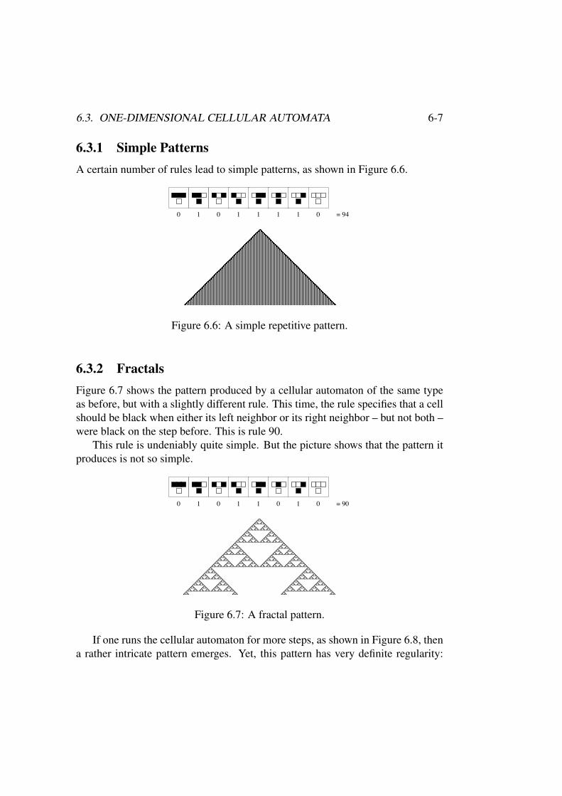
6.3.1 Simple PatternsA certain number of rules lead to simple patterns, as shown in Figure 6.6.

01111010 = 94

Figure 6.6: A simple repetitive pattern.

6.3.2 FractalsFigure 6.7 shows the pattern produced by a cellular automaton of the same typeas before, but with a slightly different rule. This time, the rule specifies that a cellshould be black when either its left neighbor or its right neighbor – but not both –were black on the step before. This is rule 90.

This rule is undeniably quite simple. But the picture shows that the pattern itproduces is not so simple.

01011010 = 90

Figure 6.7: A fractal pattern.

If one runs the cellular automaton for more steps, as shown in Figure 6.8, thena rather intricate pattern emerges. Yet, this pattern has very definite regularity:


it actually consists of many nested triangular pieces that all have the same from.Each of these pieces is essentially just a smaller copy of the whole pattern, withstill smaller copies nested in a very regular way inside it.

Pattern with nested structure of this kind are often called fractals or self-similar.

(a)

(b)

Figure 6.8: Larger versions of the pattern shown in Figure 6.7, obtained after(a) 1000 time steps and (b) 2500 time steps.


6.3.3 ChaosIt seems, from the patterns we have observed so far, that cellular automata withrules as simple as the ones we have been using can only yield patterns that arehighly regular: either uniform or repetitive patterns, or nested fractal-like patterns.

The remarkable fact is that this turns out to be wrong. Figure 6.9 shows thepattern produced using rule 30 and starting again with just one single black cell.Rather then getting a simple regular pattern as we might expect, the cellular au-tomaton instead produces a pattern that seems extremely irregular and complex.

01111000 = 30

Figure 6.9: A chaotic pattern.

Some regularity can be seen (especially on the left-hand side of the pattern),and it is possible to predict some global features of the pattern (for instance, blackand white will on average always occur equally often).

Yet, there are no signs of overall regularity (see Figure 6.10). Even though thesystem is perfectly deterministic, the behavior looks almost random! For example,one can look at the sequence of colors directly below the initial black cell. And, atleast in the first million steps in this sequence, it never repeats, and no statisticalmethods of analysis shows any meaningful deviation from perfect randomness. Infact, this property motivated Stephen Wolfram to use this rule as a pseudo randomnumber generator in its own program Mathematica.

One can wonder where this complexity comes from. We certainly did not putit into the system in any direct way when we set it up. For we just used a simplecellular automaton rule, and just started from a simple initial condition containinga single black cell.

This result illustrates a basic principle of complex systems: simple determin-istic systems, composed of many elements, can produce astonishingly complexbehaviors.


Figure 6.10: Larger versions of the pattern shown in Figure 6.9, obtained after1000 time steps.


Because of this, Wolfram believes that rule 30, and cellular automata in gen-eral, are the key to understanding how simple rules produce complex structuresand behaviour in nature. For instance, a pattern resembling rule 30 appears on theshell of the widespread cone snail species conus textile (see Figure 6.11).

Figure 6.11: The cone snail species conus textile exhibits a cellular automata pat-tern on its shell.

6.3.4 Edge of ChaosThe pattern produced by rule 30, despite its complexity, displays neverthelesssome regularities (see Figure 6.10). For instance, stripes can be seen on the left-hand side of the pattern, but never appear on the right-hand side.

It turns out that there are cellular automata whose behavior is in effect stillmore complex – and in which even such global features of the pattern becomevery difficult to predict.

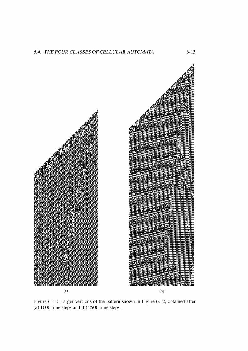
Rule 110 gives a rather dramatic example. Figure 6.12 shows that this cellularautomata produces a pattern which is neither highly regular, nor completely ran-dom. Indeed, when looking at the pattern produced after 1000 time steps as shownin Figure 6.13(a), a remarkable mixture of regularity and irregularity can be ob-served. On the left-hand side, there are diagonal stripes that occur at intervals ofexactly 80 steps. But on the right-hand side, some complex patterns seems to de-


01110110 = 110

Figure 6.12: A pattern which seems neither highly regular nor completely random.

velop, move at different speeds, interact and even leave traces. Even more surpris-ing is that the complex pattern that seems to develop in Figure 6.13(a) “suddenly”vanishes almost completely after 2500 time steps, as shown in Figure 6.13(b).

This kind of systems, which seems to lie on the “edge of chaos”, possessesinteresting properties that will be discussed later in this chapter.

6.4 The Four Classes of Cellular AutomataIn the previous section, we saw how a very simple kind of cellular automata could,despite the extreme simplicity of the underlying mechanism, produce some quiteremarkable behaviors. In this section, we will examine what happens in generalwith arbitrary cellular automata when started from random initial conditions.

One could expect that such a general question does not have any useful answer.Indeed, every single cellular automaton after all has a different underlying rule,with different properties and potentially different consequences – some of whichhave already been illustrated in the previous section.

Interestingly, looking at many patterns produced by various cellular automatawill reveal something quite remarkable. Even though each pattern is differentin detail, the number of fundamentally different types of patterns is very limited.Wolfram (1984) proposed a classification scheme which divided cellular automatarules into four categories.

In what follows, the four classes of cellular automata will be illustrated withthe same kind of cellular automata that we’ve used so far. Note however that thisclassification also holds for other arbitrary, more general cellular automata (i.e.with larger neighborhood, more states and higher dimensions).

6.4. THE FOUR CLASSES OF CELLULAR AUTOMATA 6-13

(a) (b)

Figure 6.13: Larger versions of the pattern shown in Figure 6.12, obtained after(a) 1000 time steps and (b) 2500 time steps.


6.4.1 Class 1Figure 6.14 illustrates different patterns produced by cellular automata of class 1.In this class, the behavior is very simple, and almost all initial conditions lead toexactly the same uniform final state.

Such systems evolve to simple “limit points” in phase space (a point being oneparticular configuration, such as all cell in state 0), and are thus said to have pointattractors.

6.4.2 Class 2Patterns produced by cellular automata belong to class 2 are shown in Figure 6.15.In this class, there are many different possible final states, but all of them consistjust of a certain set of simple structures that either remain the same forever, orrepeat every few steps.

Such systems evolve to “limit cycles”, and are thus said to have periodic at-tractors.

6.4.3 Class 3In class 3, illustrated in Figure 6.16, the behavior is more complicated, and seemsin mayn respects random, although triangles and other small-scale structures areessentially always at some level seen.

Such systems are said to have strange or chaotic attractors.

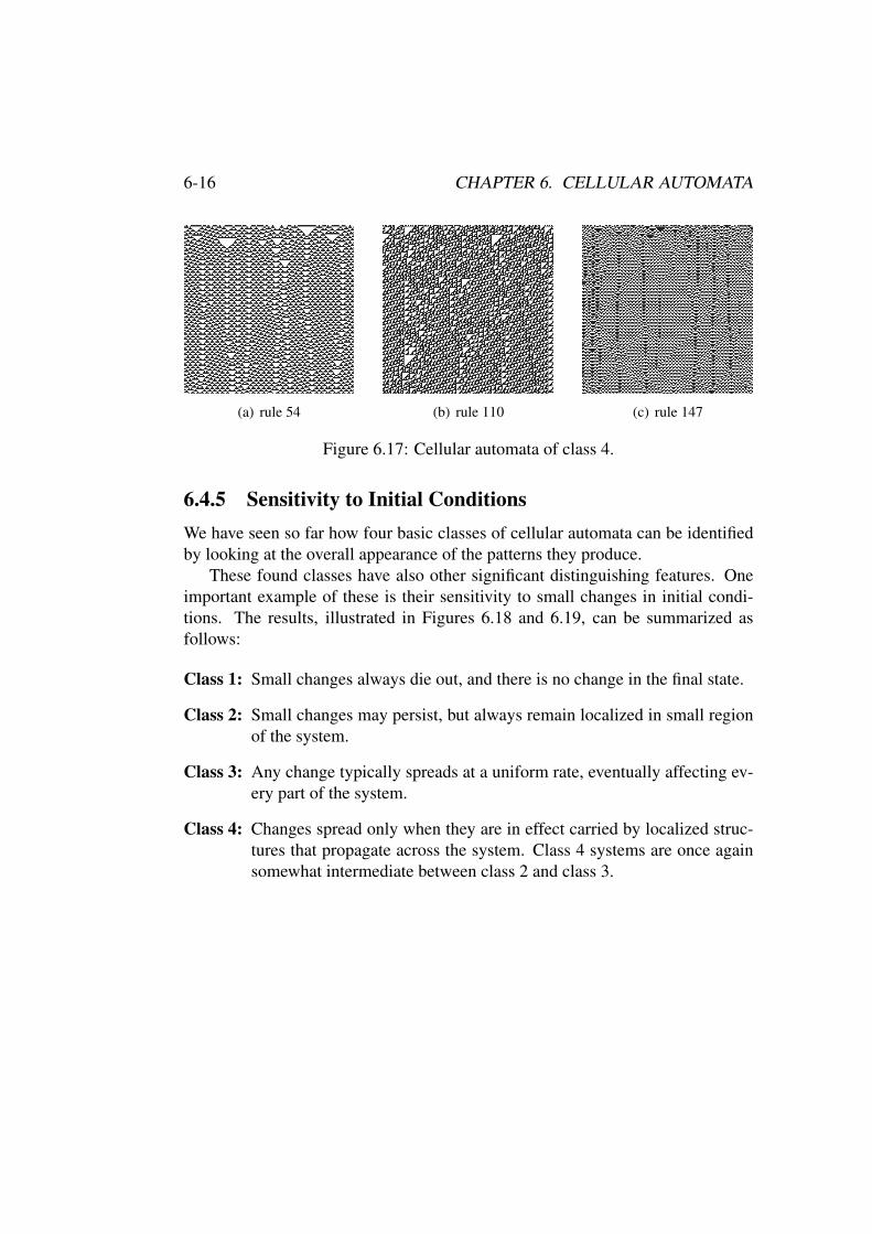
6.4.4 Class 4Class 4 correspond to the “edge of chaos” between class 2 and class 3. It involvesa mixture of order and randomness: localized structures are produced which ontheir own are failry simple, but these structures move around and interact witheach other in very complicated ways (see Figure 6.17).


(a) rule 128 (b) rule 168 (c) rule 250

Figure 6.14: Cellular automata of class 1.








6.4.5 Sensitivity to Initial ConditionsWe have seen so far how four basic classes of cellular automata can be identifiedby looking at the overall appearance of the patterns they produce.

These found classes have also other significant distinguishing features. Oneimportant example of these is their sensitivity to small changes in initial condi-tions. The results, illustrated in Figures 6.18 and 6.19, can be summarized asfollows:

Class 1: Small changes always die out, and there is no change in the final state.

Class 2: Small changes may persist, but always remain localized in small regionof the system.

Class 3: Any change typically spreads at a uniform rate, eventually affecting ev-ery part of the system.

Class 4: Changes spread only when they are in effect carried by localized struc-tures that propagate across the system. Class 4 systems are once againsomewhat intermediate between class 2 and class 3.


(a) Class 1 (b) Class 2

(c) Class 3 (d) Class 4

Figure 6.18: The effect of changing the color of a single cell in the initial condi-tions for typical cellular automata from each of the four classes. The black dotsindicate all the cells that change. (Wolfram, 2002, p. 250)


Figure 6.19: 1 cell changed in a cellular automata belonging to class 4. (Wolfram,2002, p. 254)


6.4.6 Langton’s ! ParameterChristopher Langton was interested in classifying the patterns of different cellularautomata. His idea relies on the following intuition. If most of the entries ina rule table of a cellular automata are zero, then the pattern will most probablyalways converge to the empty configuration. The more entries in the rule tableare different from zero, higher is the probability of obtaining complex or chaoticpatterns.

This qualitative statement can be defined more formally using the ! parameter,which Langton (1990) defined as:

! =N " n0

N

where N is the number of entries in the rule table of a cellular automaton, and n0

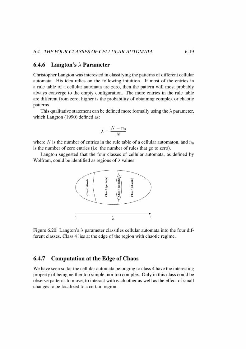
is the number of zero entries (i.e. the number of rules that go to zero).Langton suggested that the four classes of cellular automata, as defined by

Wolfram, could be identified as regions of ! values:

Cla

ss 1

(fi

xed

)

Cla

ss 2

(p

erio

dic

)

Cla

ss 4

(co

mp

lex)

Cla

ss 3

(ch

aoti

c)

!10

Figure 6.20: Langton’s ! parameter classifies cellular automata into the four dif-ferent classes. Class 4 lies at the edge of the region with chaotic regime.

6.4.7 Computation at the Edge of ChaosWe have seen so far the cellular automata belonging to class 4 have the interestingproperty of being neither too simple, nor too complex. Only in this class could beobserve patterns to move, to interact with each other as well as the effect of smallchanges to be localized to a certain region.


By viewing such moving patterns as bits of information being transmitted,stored and modified, Langton (1990) showed that the optimal conditions for thesupport of computation is found at the phase transition between the non-chaoticregime and the chaotic regime. In fact, Cook (2004) has proven that rule 110is capable of universal computation, i.e. has the same computational power as a(universal) Turing machine!4

Langton was thus the first to coin the term of “computation at the edge ofchaos”. It is interesting to note that this idea has been followed in some quitedifferent area, namely by Stuart Kauffman in the theory of biological evolution.Kauffman (1993) suggests that life exists at the edge of chaos – somewhere be-tween chemical reactions that do not produce anything interesting and systemsthat are chemically too reactive.

6.5 The Game of LifeRather than further exploring all kind of cellular automata with increasing dimen-sionality (so far, we have only illustrated 1-dimensional cellular automata), wewill concentrate in this section on one particular 2-dimensional cellular automa-ton called the “game of life” invented by thee British mathematician John Conwayin 1970.

Each cell of this cellular automaton can be in either one of two states, called“dead” or “alive”, and obeys the following very simple set of rules:

Loneliness:If a living cell has less than two neighbors, then it dies.

Overcrowding:If a living cell has more than three neighbors, then it dies.

Reproduction:If a dead cell has exactly three living neighbors, then it comes to life.

Stasis:Otherwise, a cell stays as it is.

4This fact may not be as surprising as it first sounds when we consider that a Turing machineis actually nothing more than a finite state automaton that can move along, read from and write onan infinite tape.

6.5. THE GAME OF LIFE 6-21

Figure 6.21: A typical state of the Game of Life.

The “game” is actually a zero-player game, meaning that its evolution is de-termined by its initial state, needing no input from human players. One interactswith the Game of Life by creating an initial configuration and observing how itevolves (see Figure 6.21).

Observing how patterns of cells evolve is highly captivating – and has indeedattracted much interest since its first public appearance. Some patterns will grow,some other will collide and die – much resembling real life processes.

6.5.1 Simple PatternsMany different types of patterns occur in the Game of Life, including static pat-terns (“still lifes”), repeating patterns (“oscillators”), and patterns that repeat them-selves after a fixed sequence of states and translate themselves across the board(“spaceships”). Common examples of these three classes are illustrated in Fig-ure 6.22.


6.5.2 Growing PatternsPatterns called “Methuselahs” can evolve for long periods before disappear orstabilize (see Figure 6.23).

Conway originally conjectured that no pattern can grow indefinitely – i.e., thatfor any initial configuration with a finite number of living cells, the populationcannot grow beyond some finite upper limit. In the game’s original appearance in“Mathematical Games”, Conway offered a $50 (!) prize to the first person whocould prove or disprove the conjecture before the end of 1970. The prize waswon in November of the same year by a team from the Massachusetts Institute ofTechnology, led by Bill Gosper; the “Gosper gun” shown in Figure 6.24 producesa glider every 30 generation. This first glider gun is still the smallest one known.

6.5.3 Universal ComputationLooking at the Game of Life from a computational point of view, gliders can beseen as bits of information being transmitted, glider guns as input to the system,and other static objects as providing the structure for the computation. For in-stance, Figure 6.25 illustrates how any logical primitive can be implemented inthe Game of Life.

More generally, it has been shown that the Game of Life is Turing complete,i.e. that it can compute anything that a universal Turing machine can compute.

Furthermore, a pattern can contain a collection of guns that combine to con-struct new objects, including copies of the original pattern. A “universal construc-tor” can be built which contains a Turing complete computer, and which can buildmany types of complex objects – including more copies of itself!

6.5. THE GAME OF LIFE 6-23

(a)

t = 0 t = 1

(b)

t = 0 t = 1 t = 2 t = 3 t = 4

(c)

Figure 6.22: Simple patterns occurring in the Game of Life. (a) Still lifes. (b) A2-periodic oscillator. (c) A “glider”, one of the simplest spaceships.

(a) (b)

Figure 6.23: Simple patterns that grow. (a) “Diehard” is a pattern that eventuallydisappears after 130 generations, or steps. (b) “Acorn” takes 5206 generations togenerate at least 25 gliders and stabilise as many oscillators.

(a) (b)

Figure 6.24: The “Gosper” glider gun. (a) Initial configuration. (b) The glidergun in action.


Figure 6.25: Logical operations implemented in the Game of Life. The streamsof gliders represent the input of the system, and the presence or absence of gliderat the very bottom the binary output of the logical operation.

6.6. COMPUTATION AND DECIDABILITY 6-25

6.6 Computation and DecidabilityWe have seen many examples – first in Chapter 3, and twice in the present chapter– of how the concept a finite state automaton could be simply extended to obtaina machine capable of “universal” computation5.

Yet, there is also a consequence to such computational power – analogous tothe insolubility of the halting problem for Turing machines: such systems are ingeneral unpredictable.

There are important limitations on predictions, which may be madefor the behavior of systems capable of universal computation. Thebehavior of such systems may in general be determined in detail es-sentially only by explicit simulation. [...] No finite algorithm or pro-cedure may be devised capable of predicting detailed behavior in acomputationally universal system. Hence, for example, no general fi-nite algorithm can predict whether a particular initial configuration ina computationally universal cellular automaton will evolve to the nullconfiguration after a finite time, or will generate persistent structures,so that sites with nonzero values will exist at arbitrarily large times.(Wolfram, 1984, p. 31)

6.6.1 Langton’s AntTo conclude this chapter, let us illustrate the problem of predictability with a sys-tem that surely astonishes anyone who first observe it.

Langton’s ant is another type of very simple cellular automaton. Squares ona plane are colored variously either black or white. We arbitrarily identify onesquare as the “ant”. The ant can travel in any of the four cardinal directions ateach step it takes. The ant moves according to the following rules:

• At a black square, turn 90" right, flip the color of the square, and moveforward one unit.

• At a white square, turn 90" left, flip the color of the square, and move for-ward one unit.

5Remember that universal “only” means capable of computing anything that a Turing machinecan compute.


These simple rules lead to surprisingly complex behavior. For instance, the be-havior of the ant starting on an empty plane is apparently chaotic, until about tenthousand steps – when suddenly the ant starts building a “highway”, a recurrentpattern of 104 steps that repeats indefinitely.

It seems that any initial configurations converge to similar repetitive patterns,suggesting that the “highway” is an attractor of Langton’s ant. But to our known-ledge, no one has been able to prove that this is true, nor to give a theoreticalexplanation for this phenomenon.

6.7 Chapter Summary• Cellular Automata are systems composed of simple finite state automata

obeying local rules.

• Cellular automata are simple examples of complex systems that can displayvery interesting behaviors, including fractals, randomness, chaos and self-organization.

• Cellular automata can be classified into four classes as suggested by StephenWolfram. These four classes correspond to different patterns observed, andto different sensitivity to initial conditions.

• Universal computation can be found at the edge of chaos, i.e. at the phasetransition between ordered and chaotic regimes.

• The are even extremely simple systems – such as Langton’s ant – that illus-trate the serious limitation of decidability or predictability with “complex”systems.

part iii complex systems, chaos and fractals · cellular automata 6.1 why study cellular automata?...

Documents