part 4: time series ii - home | yu/class/ess210b/lecture.5.eof.all.pdf · part 4: time series ii...

ESS210BESS210BProf. JinProf. Jin--Yi YuYi Yu

Part 4: Time Series IIPart 4: Time Series II

EOF Analysis

Principal Component

Rotated EOF

Singular Value Decomposition (SVD)


Empirical Orthogonal Function AnalysisEmpirical Orthogonal Function Analysis

Empirical Orthogonal Function (EOF) analysis attempts to find a relatively small number of independent variables (predictors; factors) which convey as much of the original information as possible without redundancy.

EOF analysis can be used to explore the structure of the variability within a data set in a objective way, and to analyze relationships within a set of variables.

EOF analysis is also called principal component analysis or factor analysis.


What Does EOF Analysis do?What Does EOF Analysis do?In brief, EOF analysis uses a set of orthogonal functions (EOFs) to represent a time series in the following way:

Z(x,y,t) is the original time series as a function of time (t) and space (x, y).

EOF(x, y) show the spatial structures (x, y) of the major factors that can account for the temporal variations of Z.

PC(t) is the principal component that tells you how the amplitude of each EOF varies with time.


EOF-1 50%PC1

t

1900 1998

EOF-2 20%t

PC2

EOF-3

••••

9%t

PC3

EOF-n <1%

Feb., 1900

Dec., 1998

•••

Nov., 1998

•

Jan., 1900 SST

99 * 12 = 1188 maps

EOF

Analysis

Principal Component

EOF (Eigen Vector)

Eigen Value

What Do You Get from EOF?What Do You Get from EOF?


An ExampleAn Example

Principal Component

Leading EOF ModeWe apply EOF analysis to a

50-year long time series of Pacific SST variation from a model simulation.

The leading EOF mode shows a ENSO SST pattern. The EOF analysis tells us that ENSO is the dominant process that produce SST variations in this 50-year long model simulation.

The principal component tells us which year has a El Nino or La Nina, and how strong they are.


Another View of the RotationAnother View of the Rotation(from Hartmann 2003)

PC1


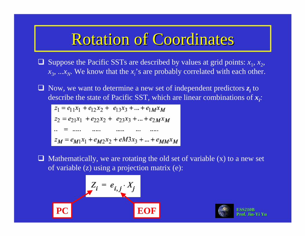
Rotation of Coordinates Rotation of Coordinates Suppose the Pacific SSTs are described by values at grid points: x1, x2, x3, ...xN. We know that the xi’s are probably correlated with each other.

Now, we want to determine a new set of independent predictors zi to describe the state of Pacific SST, which are linear combinations of xi:

Mathematically, we are rotating the old set of variable (x) to a new set of variable (z) using a projection matrix (e):

PC EOF


Determine the Projection CoefficientsDetermine the Projection CoefficientsThe EOF analysis asks that the projection coefficients are determined in such a way that:(1) z1 explains the maximum possible amount of the variance of the x’s;(2) z2 explains the maximum possible amount of the remaining variance

of the x’s;(3) so forth for the remaining z’s.

With these requirements, it can be shown mathematically that theprojection coefficient functions (eij) are the eigenvectors of the covariance matrix of x’s.

The fraction of the total variance explained by a particular eigenvector is equal to the ratio of that eigenvalue to the sum of all eigenvalues.

the orthogonal requirement in time !


Eigenvectors of a Symmetric MatrixEigenvectors of a Symmetric Matrix

Any symmetric matrix R can be decomposed in the following way through a diagonalization, or eigenanalysis:

Where E is the matrix with the eigenvectors ei as its columns, and L is the matrix with the eigenvalues λi, along its diagonal and zeros elsewhere.

The set of eigenvectors, ei, and associated eigenvalues, λi, represent a coordinate transformation into a coordinate space where the matrix R becomes diagonal.


Covariance MatrixCovariance MatrixThe EOF analysis has to start from calculating the covariance matrix.

For our case, the state of the Pacific SST is described by values at model grid points Xi.

Let’s assume the observational network in the Pacific has 10 grids in latitudinal direction and 20 grids in longitudinal direction, then there are 10x20=200 grid points to describe the state of pacific SST. So we have 200 state variables:

Xm(t), m =1, 2, 3, 4, …, 200

In our case, there are monthly observations of SSTs over these 200 grid points from 1900 to 1998. So we have N (12*99=1188) observations at each Xm:

Xmn = Xm(tn), m=1, 2, 3, 4, …., 200n=1, 2, 3, 4, ….., 1188


Covariance Matrix Covariance Matrix –– cont.cont.The covariance between two state variables Xi and Xj is:

The covariance matrix is as following:

Here N = 1188

X12 X1,M-1 X1MX11 X13 •••••X22 X2,M-1 X2,MX21 X23 •••••X32 X3,M-1 X3,MX31 X33 •••••

XM-1,2 XM-1,M-1 XM-1,MXM-1,1 XM-1,3 •••••XM,2 XM,M-1 XM,MXM,1 XM,3 •••••

Here M= 200


Eigenvectors of a Symmetric MatrixEigenvectors of a Symmetric Matrix

Any symmetric matrix R can be decomposed in the following way through a diagonalization, or eigenanalysis:

Where E is the matrix with the eigenvectors ei as its columns, and L is the matrix with the eigenvalues λi, along its diagonal and zeros elsewhere.

The set of eigenvectors, ei, and associated eigenvalues, λi, represent a coordinate transformation into a coordinate space where the matrix R becomes diagonal.


Orthogonal ConstrainsOrthogonal ConstrainsThere are orthogonal constrains been build in in the EOF analysis:

(1) The principal components (PCs) are orthogonal in time.There are no simultaneous temporal correlation between any two principal components.

(2) The EOFs are orthogonal in space.There are no spatial correlation between any two EOFs.

The second orthogonal constrain is removed in the rotated EOF analysis.


Mathematic BackgroundMathematic Background

I don’t want to go through the mathematical details of EOF analysis. Only some basic concepts are described in the following few slids.

Through mathematic derivations, we can show that the empirical orthogonal functions (EOFs) of a time series Z(x, y, t) are the eigenvectors of the covarinace matrix of the time series.

The eigenvalues of the covariance matrix tells you the fraction of variance explained by each individual EOF.


Some Basic Matrix OperationsSome Basic Matrix OperationsA two-dimensional data matrix X:

The transpose of this matrix is XT:

The inner product of these two matrices:


How to Get Principal Components?How to Get Principal Components?

If we want to get the principal component, we project a single eigenvector onto the data and get an amplitude of this eigenvector at each time, eTX:

For example, the amplitude of EOF-1 at the first measurement time is calculated as the following:


Using SVD to Get EOF&PCUsing SVD to Get EOF&PC

We can use Singular Value Decomposition (SVD) to get EOFs, eigenvalues, and PC’s directly from the data matrix, without the need to calculate the covariance matrix from the data first.

If the data set is relatively small, this may be easier than computing the covariance matrices and doing theeigenanalysis of them.

If the sample size is large, it may be computationally more efficient to use the eigenvalue method.


What is SVD?What is SVD?

Any m by n matrix A can be factored into

The columns of U (m by m) are the EOFs

The columns of V (n by n) are the PCs.

The diagonal values of Σ are the eigenvalues represent the amplitudes of the EOFs, but not the variance explained by the EOF.

The square of the eigenvalue from the SVD is equal to the eigenvalue from the eigen analysis of the covariance matrix.

original time series EOFs

normalized PCs


An Example An Example –– with SVD methodwith SVD method

(from Hartmann 2003)


An Example An Example –– With With EigenanalysisEigenanalysis



Correlation MatrixCorrelation MatrixSometime, we use the correlation matrix, in stead of the covariance matrix, for EOF analysis.

For the same time series, the EOFs obtained from the covariance matrix will be different from the EOFs obtained from the correlation matrix.

The decision to choose the covariance matrix or the correlation matrix depends on how we wish the variance at each grid points (Xi) are weighted.

In the case of the covariance matrix formulation, the elements of the state vector with larger variances will be weighted more heavily.

With the correlation matrix, all elements receive the same weight and only the structure and not the amplitude will influence the principal components.


Correlation Matrix Correlation Matrix –– cont.cont.

The correlation matrix should be used for the following two cases:

(1)The state vector is a combination of things with different units.

(2) The variance of the state vector varies from point to point so much that this distorts the patterns in the data.


Presentations of EOF Presentations of EOF –– Variance MapVariance Map

There are several ways to present EOFs. The simplest way is to plot the values of EOF itself. This presentation can not tell you how much the real amplitude this EOF represents.

One way to represent EOF’s amplitude is to take the time series of principal components for an EOF, normalize this time series to unit variance, and then regress it against the original data set.

This map has the shape of the EOF, but the amplitude actually corresponds to the amplitude in the real data with which this structure is associated.

If we have other variables, we can regress them all on the PC of one EOF and show the structure of several variables with the correctamplitude relationship, for example, SST and surface vector windfields can both be regressed on PCs of SST.


Presentations of EOF Presentations of EOF –– Correlation MapCorrelation Map

Another way to present EOF is to correlate the principal component of an EOF with the original time series at each data point.

This way, present the EOF structure in a correlation map.

In this way, the correlation map tells you what are the co-varying part of the variable (for example, SST) in the spatial domain.

In this presentation, the EOF has no unit and is non-dimensional.


How Many How Many EOFs EOFs Should We Retain?Should We Retain?

There are no definite ways to decide this. Basically, we look at the eigenvalue spectrum and decide:

(1) The 95% significance errors in the estimation of the eigenvalues is:

If the eigenvalues of adjacent EOF’s are closer together than this standard error, then it is unlikely that their particular structures are significant.

(2) Or we can just look at the slope of the eigenvalue spectrum.We would look for a place in the eigenvalue spectrum where it levels off so that successive eigenvalues are indistinguishable. We would not consider any eigenvectors beyond this point as being special.

effective numbers of degree of freedom


An ExampleAn Example

The first EOF is wellseparated from the rest EOF modes



Rotated EOFRotated EOFThe orthogonal constrain on EOFs sometime cause the spatial structures of EOFS to have significant amplitudes all over the spatial domain.

We can not get localized EOF structures.Therefore, we want to relax the spatial orthogonal constrain on EOFs (but still keep the temporal orthogonal constrain).We apply the Rotated EOF analysis.

To perform the rotated EOF analysis, we still have to do the regular EOF first.

We then only keep a few EOF modes for the rotation.We “rotated” these selected few EOFs to form new EOFs (factors).based on some criteria.These criteria determine how “simple” the new factors are.


Criteria for the RotationCriteria for the Rotation

Basically, the criteria of rotating EOFs is to measure the “simplicity” of the EOF structure.

Basically, simplicity of structure is supposed to occur when most of the elements of the eigenvector are either of order one (absolute value) or zero, but not in between.

There are two popular rotation criteria:(1) Quartimax Rotation(2) Varimax Rotation


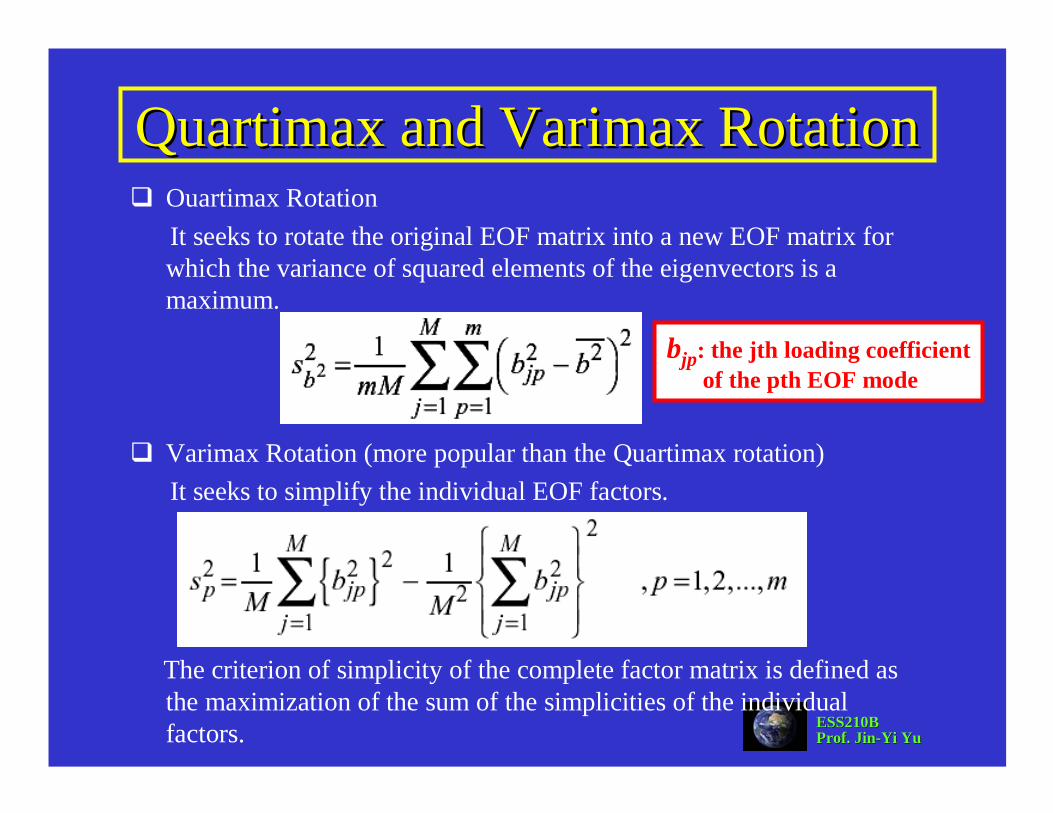
Quartimax Quartimax and and Varimax Varimax RotationRotationOuartimax RotationIt seeks to rotate the original EOF matrix into a new EOF matrix for which the variance of squared elements of the eigenvectors is a maximum.

Varimax Rotation (more popular than the Quartimax rotation)It seeks to simplify the individual EOF factors.

The criterion of simplicity of the complete factor matrix is defined as the maximization of the sum of the simplicities of the individual factors.

bjp: the jth loading coefficientof the pth EOF mode


Reference For the Following ExamplesReference For the Following Examples

The following few examples are from a recent paper published on Journal of Climate:

Dommenget, D. and M. Latif (2002): A Cautionary Note A Cautionary Note onon the Interpretation of EOFthe Interpretation of EOF. J. Climate, Vol. 15, No.2, pages 216-225.


Example 1:Example 1:Atlantic SST Atlantic SST VariabilityVariability

RotatedEOF

LinearRegression

EOF

From Dommenget, D. and M. Latif (2002)


Example 2: Indian Ocean SST VariabilityExample 2: Indian Ocean SST Variability

RotatedEOF

LinearRegression

EOF



Example 3:Example 3:SLP VariabilitySLP Variability

(Arctic Oscillation)(Arctic Oscillation)

RotatedEOF

LinearRegression

Covariance-BasedEOF

Correlation-BasedEOF



Example 4:Example 4:LowLow--Dimensional Dimensional

Variability Variability (Variance Based)(Variance Based)

Rotated EOF

Linear Regression

Physical Modes

EOF



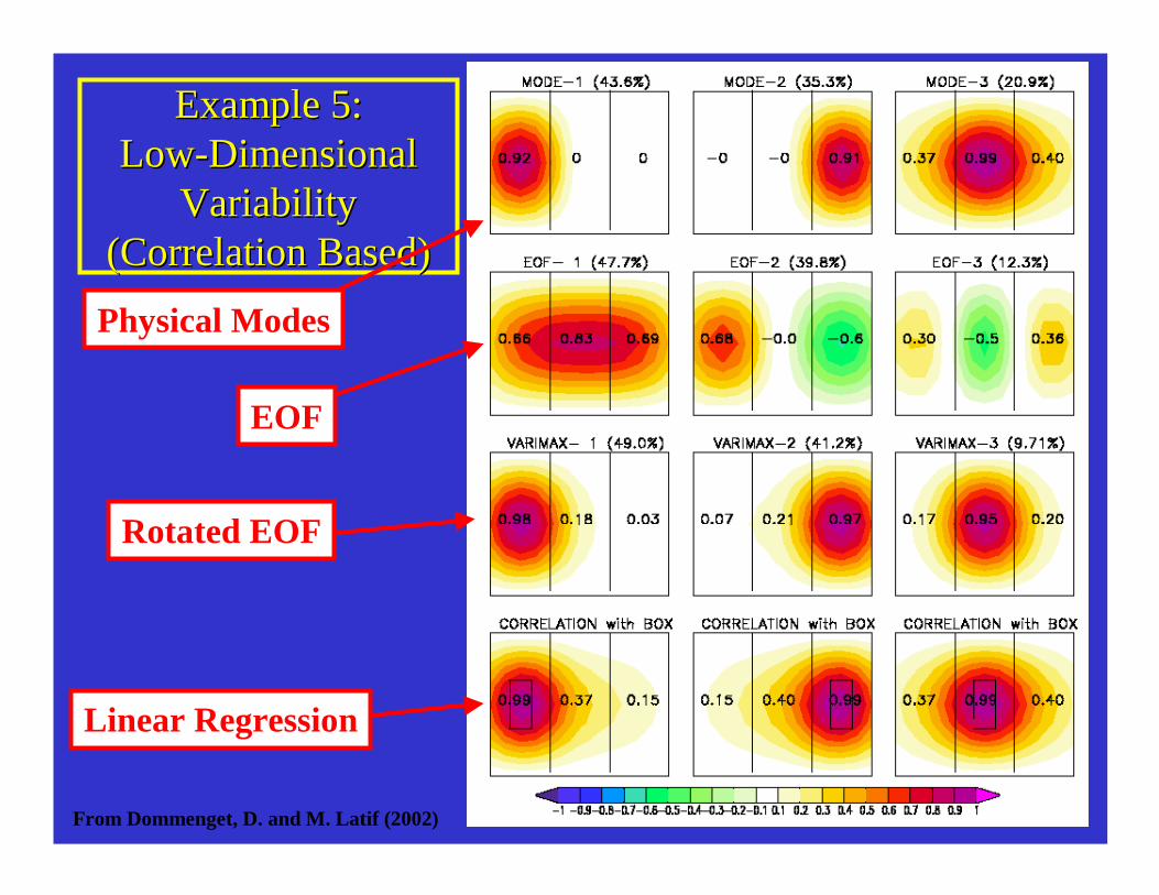
Example 5:Example 5:LowLow--Dimensional Dimensional

Variability Variability (Correlation Based)(Correlation Based)

Rotated EOF

Linear Regression

Physical Modes

EOF



Correlated Structures between Two VariablesCorrelated Structures between Two Variables

SVD analysis is also used to reveal the correlated spatial structures between two different variables or fields, such as the interaction structures between the atmosphere and oceans.

We begin by constructing the covariance matrix between data matrices X and Y of size MxN and LxN, where M and L are the structure dimensions and N is the shared sampling dimension.

Their covariance matrix is:

or in matrix form:


An Example An Example –– SVD (SST, SLP)SVD (SST, SLP)

Sea Surface Temperature (SST)

Sea Level Pressure (SLP)


SVD Analysis of Covariance MatrixSVD Analysis of Covariance MatrixWe then apply the SVD analysis to the covariance matrix and obtain:

U: The columns of U (MxM) are the column space of CXY and represent the structures in the covariance field of X.

V: The columns of V are the row space of CXY and are those structures in the Y space that explain the covariance matrix.

Σ: The singular values are down the diagonal of the matrix Σ. The sum of the squares of the singular values is equal to the sum of the squared covariances between the original elements of X and Y.

MxL MxM MxL LxL


What Do What Do UU and and VV mean?mean?The column space (in U) will be structures in the dimension M that are orthogonal and have a partner in the row space of dimension L (in V).

Together these pairs of vectors efficiently and orthogonallyrepresent the structure of the covariance matrix.

The hypothesis is that these pairs of functions represent scientifically meaningful structures that explain the covariance between the two data sets.

The 1st EOF in U and the 1st EOF in V together explain the most of the covariance (correlation) between two variables X and Y.


Principal ComponentsPrincipal ComponentsThe principal components corresponding to the EOFs in Uand V can be obtained by projecting the EOFs (singular vectors) onto the original data:

The covariance between each pair (kth) of the principal component should be equal to their corresponding singular value.


Presentation of SVD VectorsPresentation of SVD VectorsSimilar to the EOS analysis, the singular vectors are normalized and non-dimensional, whereas the expansion coefficients have the dimensions of the original data.

To include amplitude information in the singular vectors, we canregress (ore correlate) the principal components of U or V with the original data for this purpose.

(1) For example, normalize the principal component of U.

(2) Regress this normalized principal component with the original data set Y to produce a “heterogeneous regression map”. This map shows the amplitude of covariance between X and Y.

(3) Regress this normalized principal component with the original data set X to produce a “homogeneous map”. This map tells us the spatial structure of X that is most correlated with Y.


Heterogeneous and Homogeneous MapsHeterogeneous and Homogeneous MapsHeterogeneous regression maps: regress (or correlate) the expansion coefficient time series of the left field with the input data for the right field, or do the same with the expansion coefficient time series for the right field and the input data for the left field.

Homogeneous regression maps: regress (or correlate) the expansion coefficient time series of the left field with the input data for the left field, or do the same with the right field and its expansion coefficients.


An Example An Example –– SVD (SST, SLP)SVD (SST, SLP)

Sea Surface Temperature (SST)

Sea Level Pressure (SLP)


SVD MapsSVD Maps

Heterogeneous Correlation Homogeneous Correlation


How to Use How to Use Matlab Matlab to do SVD?to do SVD?

See pages 27-28 of the paper “A manual for EOF and SVD analysis of climate data” by Bjornsson and Venegas.

part 4: time series ii - home | yu/class/ess210b/lecture.5.eof.all.pdf · part 4: time series ii...

Documents