PART 4. Scanning Tunneling Microscopy. Contents

PART 4. Scanning Tunneling Microscopy

Contents

1 INTRODUCTION .................................................................................................................................4-2 2 PREPARATION FOR OPERATION .................................................................................................4-3

2.1 BASIC PROCEDURE OF THE INSTRUMENT PREPARATION FOR STM OPERATION.............................4-3 2.2 ELECTROMECHANICAL CONFIGURATION .......................................................................................4-4 2.3 LOADING SCANNER CALIBRATION PARAMETERS ..........................................................................4-5 2.4 MANUFACTURING THE TIP.............................................................................................................4-7 2.5 INSTALLING THE TIP INTO THE HOLDER.........................................................................................4-8 2.6 CENTERING THE SCANNER.............................................................................................................4-9 2.7 PREPARING AND INSTALLING A SAMPLE......................................................................................4-11 2.8 INSTALLING THE MEASURING HEAD............................................................................................4-13 2.9 PERFORMING THE PRELIMINARY SAMPLE TO TIP APPROACH ......................................................4-13 2.10 INSTALLATION OF A PROTECTIVE HOOD......................................................................................4-14 2.11 INSTRUMENT TURNING ON...........................................................................................................4-15

3 CONSTANT CURRENT MODE.......................................................................................................4-16 3.1 SETTING THE INSTRUMENT FOR WORKING IN STM MODES.........................................................4-16 3.2 LANDING THE SAMPLE TO THE TIP...............................................................................................4-17 3.3 SETTING “FEEDBACK GAIN” FACTOR WORKING LEVEL..............................................................4-20 3.4 SWITCHING THE FEEDBACK SIGNAL OVER ..................................................................................4-21 3.5 SETTING THE SCANNING PARAMETERS........................................................................................4-22 3.6 SCANNING ...................................................................................................................................4-25 3.7 SAVING THE OBTAINED RESULTS ................................................................................................4-28 3.8 TERMINATION OF OPERATION......................................................................................................4-28

4 CONSTANT HEIGHT MODE. ATOMIC RESOLUTION ON GRAPHITE ...............................4-30 5 SCANNING TUNNELING SPECTROSCOPY................................................................................4-34

5.1 I(V) SPECTROSCOPY ....................................................................................................................4-34 5.2 MODULATION TECHNIQUE OF THE SCANNING TUNNELING SPECTROSCOPY.

BARRIER HEIGHT IMAGING..........................................................................................................4-35 5.2.1 SPM Mode Setup ..........................................................................................................4-35 5.2.2 Setting the Piezo-oscillator Operating Frequency........................................................4-36 5.2.3 Scanning .......................................................................................................................4-38

4-1

PART 4. Scanning Tunneling Microscopy

1 Introduction

The Scanning Tunneling Microscopy is intended for the investigation of the surfaces properties of conductive materials with resolution down to atomic scale. The tunnel current recorded during scanning is small enough (0.5 pA -50 nA) to allow investigating samples with low conductance, biological objects in particular.

Application of special modes allows to investigate the surface distribution of various electrical characteristics, such as work function, local density of electron states, etc.

One of the STM limitations is the complexity of interpretation of the obtained results, since the STM image is determined not only by the topography, but also by the local electrical characteristics.

4-2

Chapter 2. Preparation for Operation

2 Preparation for Operation

This section describes general preparation procedures to perform STM measurements.

2.1 Basic Procedure of the Instrument Preparation for STM Operation

Preparation of the instrument for operation using STM modes can be divided into the following basic operations:

Step 1. Electromechanical Configuration (see page 4-4)

Step 2. Loading Scanner Calibration Parameters (see page 4-5)

Step 3. When the Equivalent Scanner is used it shall be prepared for operation as described in the Attachment. (see Appendix, Part 5, Chapter 5 «Preparing Scanner for Operation with Equivalent»).

Step 4. Manufacturing the Tip (see page 4-7)

Step 5. Installing the Tip into the Holder (see page 4-8)

Step 6. Centering the Scanner (see page 4-9)

Step 7. Preparing and Installing a Sample (see page 4-11)

Step 8. Installing the Measuring Head (see page 4-13)

Step 9. Performing the Preliminary Sample to Tip Approach (see page 4-13)

Step 10 Installation of a Protective (see page 4-14)

Step 11. Instrument Turning on (sees page 4-15)

ATTENTION! Switch the controller off before connecting/disconnecting cables. Disconnecting or connecting while the device is operating may damage its electrical circuit.

4-3

PART 4. Scanning Tunneling Microscopy

2.2 Electromechanical Configuration

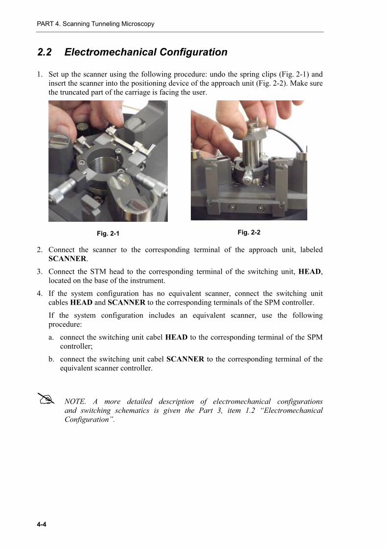
1. Set up the scanner using the following procedure: undo the spring clips (Fig. 2-1) and insert the scanner into the positioning device of the approach unit (Fig. 2-2). Make sure the truncated part of the carriage is facing the user.

Fig. 2-1

Fig. 2-2

2. Connect the scanner to the corresponding terminal of the approach unit, labeled SCANNER.

3. Connect the STM head to the corresponding terminal of the switching unit, HEAD, located on the base of the instrument.

4. If the system configuration has no equivalent scanner, connect the switching unit cables HEAD and SCANNER to the corresponding terminals of the SPM controller.

If the system configuration includes an equivalent scanner, use the following procedure:

a. connect the switching unit cabel HEAD to the corresponding terminal of the SPM controller;

b. connect the switching unit cabel SCANNER to the corresponding terminal of the equivalent scanner controller.

NOTE. A more detailed description of electromechanical configurations and switching schematics is given the Part 3, item 1.2 “Electromechanical Configuration”.

4-4

Chapter 2. Preparation for Operation

2.3 Loading Scanner Calibration Parameters

Turn on the computer and than launch the control program.

Upon starting the program the Default.par file which contains calibration parameter for a specific scanner is loaded by default. If only one scanner is supplied with the instrument then the Default.par file contains the parameters for this particular scanner.

If several scanners are included in the package then Default.par stores parameters corresponding to one of the scanners.

After changing the scanner the related parameter file (par-file) shall be loaded.

To load a par-file for the scanner complete the following operations:

1. In the Main menu select successively the following items Settings → Calibrations → Load Calibrations (Fig. 2-3).

Fig. 2-3

This will open a dialog box with a list of par-files contained in the PARFiles folder as in the example shown in Fig. 2-4.

The names of the par-files have the following pattern: zXXX.par – for exchangeable scanners;

where XXX – is the scanner number.

Fig. 2-4

2. Choose the par-file corresponding to the installed scanner.

3. Click the Open button to load the par-file.

4-5

PART 4. Scanning Tunneling Microscopy

If you prefer the current scanner parameters to load by default at the program start-up save the file as Default.par. Proceed as follows:

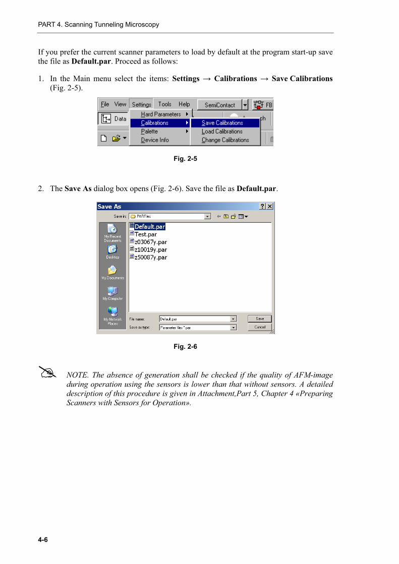
1. In the Main menu select the items: Settings → Calibrations → Save Calibrations (Fig. 2-5).

Fig. 2-5

2. The Save As dialog box opens (Fig. 2-6). Save the file as Default.par.

Fig. 2-6

NOTE. The absence of generation shall be checked if the quality of AFM-image during operation using the sensors is lower than that without sensors. A detailed description of this procedure is given in Attachment,Part 5, Chapter 4 «Preparing Scanners with Sensors for Operation».

4-6

Chapter 2. Preparation for Operation

2.4 Manufacturing the Tip

The tip is the sharpened end of a platinum-iridium (PtIr), or platinum-rhodium (PtRo) (with platinum content of about 80 %) or tungsten (W) wire, 8-10 mm long with a diameter of 0.25 - 0.5 mm.

The sharpness of the tip can be evaluated by imaging a reference sample with known surface characteristics, for example Highly Oriented Pyrolytic Graphite (HOPG).

There are two techniques of manufa

cturing an STM tip:

− By cutting the wire apex with scissor (PtIr, PtRo) (see below);

− By electrochemical etching (W, Pt, PtIr, PtRo).

The simplest STM tip manufacturing technique consists in cutting the wire apex with the scissors. In that case the apex radius of curvature is less than 10 nm.

Sharp-edged scissors and tweezers with kinks on the interior surface, to be found in the toolkit supplied with the microscope, are used to cut the wire.

ATTENTION! Do not use the wire cutting scissors for other purposes.

Fig. 2-7

4-7

PART 4. Scanning Tunneling Microscopy

Apex forming procedure:

1. Clamp the wire with the tweezers so that it projects beyond its edge for 2-3 mm (Fig. 2-7).

2. Cut the wire at an angle of 10-15 degrees as close to its apex as possible and simultaneously pull the scissors along the wire axis to separate the part being cut off. This is done to avoid the contact between the cutting edges of the scissors and the tip apex. This procedure implies rather a tearing off the wire in the last moment than truncating it. This results in a sharp apex, formed at the wire’s end (Fug. 2-8).

Fug. 2-8. Typical shape of a wire cutoff (apex of the tip)

3. Check the resulting cutoff shape using the optical microscope with 200-x magnification (if possible). Repeat the cutting process, if necessary.

ATTENTION! Avoid any contact with the tip apex in order not to damage it.

The overall length of the tip should not exceed 10 mm.

After cutting the wire you may anneal its apex in the flame of an alcohol lamp for 1-2 seconds to remove organic substances. Check the apex of the tip using the optical microscope1: the cutoff section should be bright, with no traces of black or dust.

2.5 Installing the Tip into the Holder

While installing the tip into the holder, it is convenient to use tweezers of two types: narrow tweezers with smooth tips and wide tweezers with kinks.

To insert the blunt end of the tip into the holder do the following:

1. Turn the STM head face down and place it on a plane surface.

2. Take the wide tweezers in one hand, holding the narrow one with the tip in it in the other.

ATTENTION! Avoid contacting a sharpened apex with any surfaces during installation.

3. Squeeze the pressure spring using the wide tweezers (Fig. 2-9 a).

1 This procedure is optional.

4-8

Chapter 2. Preparation for Operation

4. Insert the tip's blunt end into the holder so that the sharpened end projects beyond the edge of the holder no more than 3-4 mm (Fig. 2-9 b).

a)

b)

Fig. 2-9. Installing the tip into the holder

5. Release the spring. The tip should be fixed firmly in the holder.

NOTE. The quality of the tip sharpness and firmness of the tip fixation in the clamp are the primary factors in determining the quality of results obtained with STM.

2.6 Centering the Scanner

Before installing a sample it is recommended to adjust the scanner with respect to the measuring head so that the tip coincides approximately with the axis of the scanner. This will reduce the surface slope during scanning.

NOTE. This procedure is optional.

Scanner centering procedure:

1. Wind the manual approach knob counter-clockwise (Fig. 2-7) to move the scanner to its lowest position.

Fig. 2-10. Manual approach knob

4-9

PART 4. Scanning Tunneling Microscopy

2. Install the measuring head with its legs into the seats of the replaceable base (Fig. 2-11).

Fig. 2-11

3. Looking from a side, set the tip-sample distance to 2-3 mm, by rotating the

approaching knob (Fig. 2-10) counter-clockwise.

4. Looking from top, make the apex of the tip coincide with the axis of the scanner, using micrometric screws of the positioning device (Fig. 2-12).

Fig. 2-12. 1 – central orifice in the sample stage (sitting on the scanner axis)

2 – micrometric screws of the positioning device

5. Retract the scanner by rotating the approaching knob clockwise.

6. Take the measuring head off the replaceable base.

4-10

Chapter 2. Preparation for Operation

2.7 Preparing and Installing a Sample

To fix samples during the STM investigations special substrates with electric contact for sample biasing are used (Fig. 2-13).

Fig. 2-13. Substrate with a spring contact

Sample preparation procedure:

1. Take a clean substrate. Cut off a strip of a double-sided adhesive tape, slightly wider than the sample.

2. Stick the adhesive tape to the substrate, smooth its surface out with the back of the tweezers to remove air bubbles between the substrate and the adhesive tape.

3. Put the sample, for example, a graphite plate (HOPG), on the adhesive tape and carefully press it with tweezers in several places (not touching the area intended for the investigation) (Fig. 2-14).

NOTE. After the sample is fixed on the substrate, a noticeable vertical drift of the sample can occur within one hour (due to the slow relaxation of sticky tape). This drift should be taken into account. If a minimal drift is required due to the nature of the investigation, prepare the sample beforehand (at least in an hour before the investigation).

Fig. 2-14. Prepared substrate with a HOPG sample installed

4. To clean and smooth the graphite sample, do the following:

a. Stick a piece of the adhesive tape (slightly wider than the sample) on the surface of the graphite sample;

b. Smooth it out to remove air bubbles;

4-11

PART 4. Scanning Tunneling Microscopy

c. With an abrupt movement remove the adhesive tape together with the top layer of graphite. The molecular layers of graphite have a spalling angle in relation to the surface layer, at which the layers are easily removed. Therefore the smoothness of the surface will depend on the direction, in which you remove a layer. Find the best direction to obtain the smoothest surface and remember (or mark) it, to use it later for cleaning the surface of pyrolitic graphite samples.

5. Use tweezers to turn the contact spring, used to apply the bias voltage and fix it to the edge of the sample so that the center of the sample remains free (Fig. 2-14).

6. Install the substrate with the sample on the sample stage, sliding it in sideways under the fixing clips. The substrate is inserted in such a manner as to make the spring contact face the operator (Fig. 2-15). Make sure that the spring contact does not touch any metal parts of the tip holder.

7. Insert the voltage feeding contact terminal into BV connector on the approach unit.

ATTENTION! Switch off the controller before connecting/disconnecting any cable. Connecting or disconnecting cables while the device is operating may damage the electronic circuit.

Fig. 2-15. 1 – spring contact, 2 – BV contact terminal

4-12

Chapter 2. Preparation for Operation

2.8 Installing the Measuring Head

1. Insert the measuring head legs into the corresponding seats of the multipurpose mount (Fig. 2-16).

Fig. 2-16. Installing the STM head

2. Connect the STM head to the terminal labeled HEAD of the switching unit (if step has not been done).

2.9 Performing the Preliminary Sample to Tip Approach

1. Looking from a side, approach the sample to the tip apex to a distance of 2-3 mm, by rotating the approaching knob.

2. Looking from top, position the tip above the area intended for investigation, by rotating the positioner screws.

NOTE. It is recommended to position the sample beforehand so that the investigated area is as close to the scanner axis as possible. In case the investigated area is far from the axis, a surface sloping can occur during scanning, restricting the application of certain techniques and complicating their implementation.

3. Then, while looking from a side, reduce the distance between the sample and the tip apex down to 0.5-1 mm (Fig. 2-17).

4-13

PART 4. Scanning Tunneling Microscopy

0.5–

1 mm

Fig. 2-17. The STM tip – sample clearance after a preliminary approach

2.10 Installation of a Protective Hood

It is recommended to work with a hood in the following cases:

− if it is necessary to obtain a high resolution image in XY plane or along Z axis;

− when working at controlled temperature;

− for protection against temperature drifts;

− for reduction of acoustic noise level.

To install the protective hood proceed as follows:

1. Install the fixing clip of the measuring head cable into its holder built into the approach unit (Fig. 2-18).

Fig. 2-18. Installation of the STM head cable into its holder

4-14

Chapter 2. Preparation for Operation

2. Mount the protective hood onto the platen of the approach unit.

3. Ground the protective hood by plugging the special cable of the approach unit into the grounding jack on the hood (Fig. 2-19).

Fig. 2-19 Protective hood mounted on the approach unit 1 – grounding jack

2.11 Instrument Turning on

1. Turn on the computer and launch the control program.

2. Turn on the SPM controller with the power switch located on the front panel. If turning on is successful, a green "tick" appears in the monitor screen bottom left corner.

3. Turn on the vibration isolation system.

4-15

PART 4. Scanning Tunneling Microscopy

3 Constant Current Mode

The Constant Current Mode implies maintaining a constant value of tunnel current during scanning, using the feedback loop system. The feedback signal, fed to the Z-channel of the scanner, traces the surface topography.

To maintain the feedback while operating the instrument in STM modes, two signals are used:

Iprlow a signal proportional to the value of the tunnel current flowing through the tip. This signal is used to maintain the feedback when approaching the sample to the tip;

Iprlog a signal proportional to the logarithm of value of the tunnel current flowing through the tip. This signal is used to maintain the feedback during scanning.

3.1 Setting the Instrument for Working in STM Modes

To switch the device onto the STM modes, click the switch button, selecting the device electronic configuration and select Tunnel Current in the basic operation panel (Fig. 3-1).

Fig. 3-1

NOTE:

− The switch button, selecting the device electronic configuration can be set in one of the four states: Custom, Contact, SemiContact and Tunnel Current;

− If Tunnel Current state is set, the device will be automatically configured for measurements in STM modes: IprLog signal is switched to the feedback input, the oscillator is set to off position, and Bias V constant voltage is fed to the sample;

− If Custom state is set, the user can customize the device freely, setting up various configurations and implementing different states of the device.

4-16

Chapter 3. Constant Current Mode

3.2 Landing the Sample to the Tip

1. Open the Approach window (by pressing the Approach button on the basic operations panel) (Fig. 3-2).

Fig. 3-2

2. Check the state of the automatic Set Point parameter setup button. The

Auto SetPoint button should be switched on, as shown in Fig. 3-3.

Fig. 3-3

3. Set the Bias V parameter value to 0.1 V as shown in Fig. 3-4.

Fig. 3-4

4. Launch the approach procedure by clicking the Landing button.

As a result:

− Set Point parameter value will be automatically set to 0.1 nA;

− IprLow will be set as the feedback input signal;

− The feedback will be switched-on and Z-piezo-scanner will be fully protracted. Z-scanner protraction will be monitored in the piezotube protraction analogue indicator, located in the lower left corner of the program main window. The length of a color strip represents the level of the scanner protraction;

− The step motor will start, moving the scanner with the sample towards the tip.

4-17

PART 4. Scanning Tunneling Microscopy

5. While the approaching is in progress, observe the changes of IprLow signal in the oscilloscope window and the state of the scanner protraction indicator, waiting for the termination of the process.

After a while, if the parameters of approaching are correctly set, the approaching will stop and the following will occur:

− IprLow signal will increase up to Set Point parameter value. The feedback will drive the Z-scanner in a position at which IprLow signal is equal to Set Point signal, this position corresponding approximately to one half of the scanner protraction range;

− The length of the color strip of the indicator will shorten, taking some intermediate position (Fig. 3-5);

− The step motor will stop;

− The increase of IprLow signal up to the value of Set Point parameter will be represented on IprLow (t) trace in the oscilloscope window;

− the message "…Approach Done." will appear in the journal (pos. 2 in Fig. 3-5);

Fig. 3-5. Completing of approach procedure 1 – indicator of scanner protraction; 2 – journal

− The feedback input signal will switch onto IprLog.

4-18

Chapter 3. Constant Current Mode

Special cases

Self-oscillations

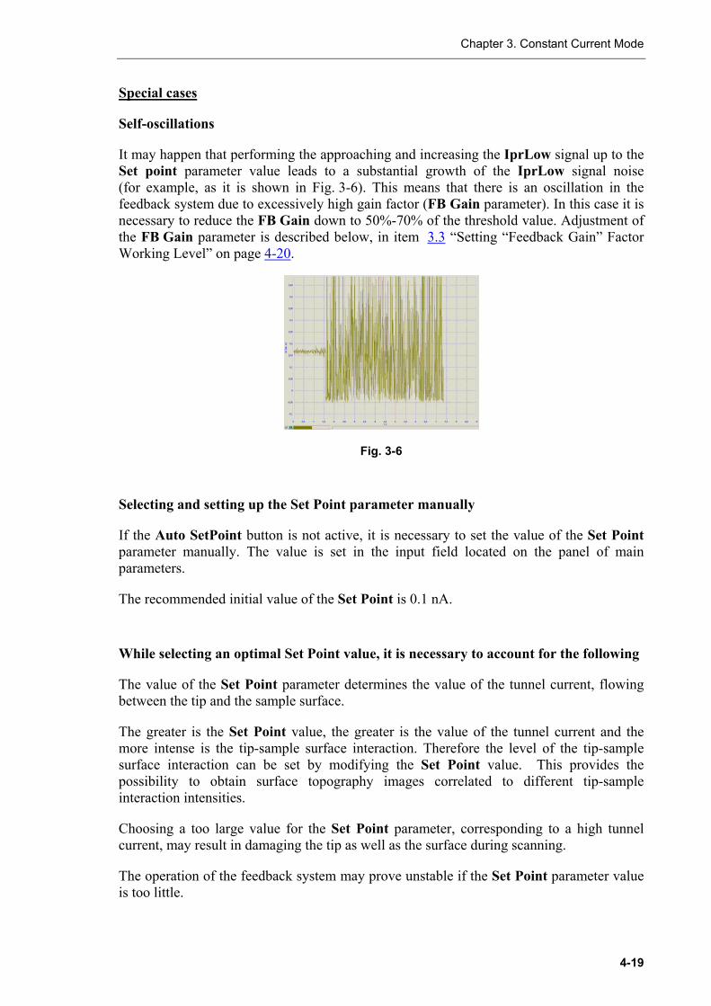
It may happen that performing the approaching and increasing the IprLow signal up to the Set point parameter value leads to a substantial growth of the IprLow signal noise (for example, as it is shown in Fig. 3-6). This means that there is an oscillation in the feedback system due to excessively high gain factor (FB Gain parameter). In this case it is necessary to reduce the FB Gain down to 50%-70% of the threshold value. Adjustment of the FB Gain parameter is described below, in item 3.3 “Setting “Feedback Gain” Factor Working Level” on page 4-20.

Fig. 3-6

Selecting and setting up the Set Point parameter manually

If the Auto SetPoint button is not active, it is necessary to set the value of the Set Point parameter manually. The value is set in the input field located on the panel of main parameters.

The recommended initial value of the Set Point is 0.1 nA.

While selecting an optimal Set Point value, it is necessary to account for the following

The value of the Set Point parameter determines the value of the tunnel current, flowing between the tip and the sample surface.

The greater is the Set Point value, the greater is the value of the tunnel current and the more intense is the tip-sample surface interaction. Therefore the level of the tip-sample surface interaction can be set by modifying the Set Point value. This provides the possibility to obtain surface topography images correlated to different tip-sample interaction intensities.

Choosing a too large value for the Set Point parameter, corresponding to a high tunnel current, may result in damaging the tip as well as the surface during scanning.

The operation of the feedback system may prove unstable if the Set Point parameter value is too little.

4-19

PART 4. Scanning Tunneling Microscopy

3.3 Setting “Feedback Gain” Factor Working Level

The larger is the gain factor (FB Gain parameter), the higher is the rate of feedback processing. However, if the gain factor is too large (let us call this value the threshold value), the operation of the feedback system becomes unstable, and the IprLow signal starts oscillating.

To provide a stable system operation, the gain factor level should be set to no more than 60%-70% of the threshold value, at which oscillation occurs.

To set the operating level of the feedback gain factor, do the following:

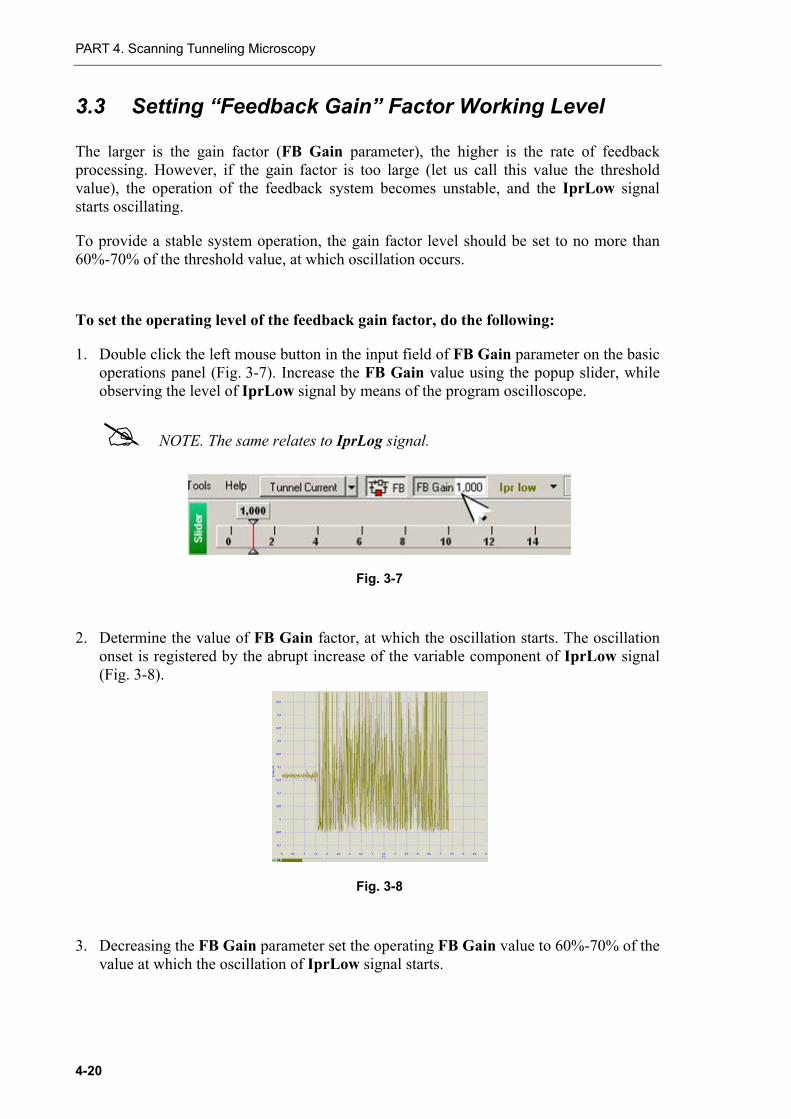
1. Double click the left mouse button in the input field of FB Gain parameter on the basic operations panel (Fig. 3-7). Increase the FB Gain value using the popup slider, while observing the level of IprLow signal by means of the program oscilloscope.

NOTE. The same relates to IprLog signal.

Fig. 3-7

2. Determine the value of FB Gain factor, at which the oscillation starts. The oscillation onset is registered by the abrupt increase of the variable component of IprLow signal (Fig. 3-8).

Fig. 3-8

3. Decreasing the FB Gain parameter set the operating FB Gain value to 60%-70% of the value at which the oscillation of IprLow signal starts.

4-20

Chapter 3. Constant Current Mode

3.4 Switching the Feedback Signal Over

The feedback may be provided by one of the two signals: IprLow or IprLog. At the sample to tip approaching the IprLow signal is used by default, whereas the IprLog signal is used during scanning. Switching over is performed automatically.

In order to manually switch over the feedback signal (for example, in scanning low-conductive samples the IprLow signal is preferable), perform the following:

1. Break the feedback loop by releasing the button (Fig. 3-9).

Fig. 3-9

2. Change the feedback input signal (Fig. 3-10).

Fig. 3-10

3. Set the value of the Set Point parameter to:

− 1 nA for IprLog signal (Fig. 3-11);

− 0.1 nA for IprLow signal.

Fig. 3-11

4. Close feedback loop by clicking the button (Fig. 3-12).

Fig. 3-12

4-21

PART 4. Scanning Tunneling Microscopy

3.5 Setting the Scanning Parameters

Open the Scan window by clicking the Scan button on the basic operations panel.

Fig. 3-13

The upper part of the SCAN window contains the scanning parameters control panel (Fig. 3-13). The oscilloscope window displaying the trace of the signal measured during scanning is located below. Still below is the scanned images viewer.

SPM Mode Setup

To set up the operating SPM mode click on Mode indicator window and select Constant Current in the drop-down menu (Fig. 3-14). The device will be configured automatically.

Fig. 3-14

Setting the scan area, number of data-points, scan resolution

Recommendations for the selection of the initial size of the scanned area:

− If some preliminary information on the sample surface properties is available, suggesting that the surface roughness does not exceed the limits of z-range of the scanner, the maximal scan size can be set;

− When data on the surface properties are not available, it is recommended to start the scanning from a smaller area, 0.5÷1 μm, for example. Based on the results of the scanning of this small area, the optimal values for Scan Rate, Set Point, FB Gain can be chosen. The scan size can then be increased.

Selecting the area of scanning:

By default, the Scan Size parameter is automatically set to maximum value. This is:

− for 10-micron scanner: 10x10 μm2;

− for 50-micron scanner: 50x50 μm2;

− for 3-micron scanner: 3x3 μm2.

4-22

Chapter 3. Constant Current Mode

To change the scan size and to select another area within the limits of the maximum possible area, perform the following:

1. Click the button in the Data Viewer toolbar (Fig. 3-15) to change the size and position of the scan area.

2. Change the area size and position using the mouse (pos. 1 in Fig. 3-15).

NOTE. Changing the scan area size will be automatically reflected in input fields of Scan Size parameter (Fig. 3-13).

3. Click the button. Make sure that the tip can touch the surface in any point within the selected area of scanning without "hitting" it anywhere. To do this click the left mouse button and, move the cursor within the limits of a selected area, keeping pressed the mouse button (pos. 2 in Fig. 3-15). The movement of the cursor reflects the actual movement of the tip relative the sample surface. The degree of piezo-scanner protraction should be controlled using the indicator at the bottom of the window.

Fig. 3-15. Data Viewer window 1 – the limits of the selected area of scanning,

2 – cursor indicating the position of the tip relative the sample surface

The selection of the area of scanning is complete.

The Interrelation of Point Number, Step Size, Scan Size Parameters:

When the Scan Size and Point Number are already set, the Step Size value is set automatically as: Step Size = (Scan Size)/(Point Number).

Modification of the Step Size parameter automatically modifies the value of the Scan Size correspondingly, whereas the value of the Point Number parameter remains the same.

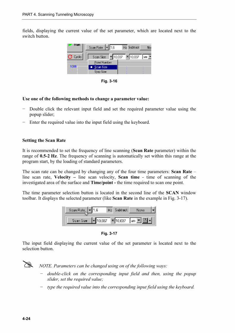
The values of the Scan Size (the size of the area of scanning), the Point Number (number of points on X and Y axes) and the Step Size (the step of scanning) parameters can be changed using the switch button displaying the selected option (Fig. 3-16) and the input

4-23

PART 4. Scanning Tunneling Microscopy

fields, displaying the current value of the set parameter, which are located next to the switch button.

Fig. 3-16

Use one of the following methods to change a parameter value:

− Double click the relevant input field and set the required parameter value using the popup slider;

− Enter the required value into the input field using the keyboard.

Setting the Scan Rate

It is recommended to set the frequency of line scanning (Scan Rate parameter) within the range of 0.5-2 Hz. The frequency of scanning is automatically set within this range at the program start, by the loading of standard parameters.

The scan rate can be changed by changing any of the four time parameters: Scan Rate – line scan rate, Velocity – line scan velocity, Scan time - time of scanning of the investigated area of the surface and Time/point - the time required to scan one point.

The time parameter selection button is located in the second line of the SCAN window toolbar. It displays the selected parameter (like Scan Rate in the example in Fig. 3-17).

Fig. 3-17

The input field displaying the current value of the set parameter is located next to the selection button.

NOTE. Parameters can be changed using on of the following ways:

− double-click on the corresponding input field and then, using the popup slider, set the required value;

− type the required value into the corresponding input field using the keyboard.

4-24

Chapter 3. Constant Current Mode

3.6 Scanning

As an example we shall consider the process of scanning of a Highly-Oriented Pyrolitic Graphite (HOPG) sample.

Scanning Start

The sample surface scanning can be started once all preparatory operations are performed, the tip is landed to the sample, the set point is selected, and the scanning parameters are set.

To start scanning click the Run button located in the left part of the SCAN window control panel.

After the Run button is pressed:

− The process of line-by-line scanning of the sample surface starts, followed by a line-by-line representation of the resulting image in the Data Viewer window (Fig. 3-18);

Fig. 3-18

− The lines of the scanned surface topography profile will be displayed one by one in the oscilloscope window (Fig. 3-18);

− Some buttons will disappear from the SCAN window control panel, replaced by a number of new ones (Fig. 3-19): Pause, Restart, Stop.

Fig. 3-19

4-25

PART 4. Scanning Tunneling Microscopy

Modifying the Parameters during Scanning

Slope subtraction:

− It is evident that the sample in the above example (Fig. 3-18) has some inclination along X axis, and correspondly the line scan exhibits a finite slope;

− The slope can be subtracted during scanning (i.e. in on-line mode), using the Subtract switch button. By default this button is in None state (Fig. 3-20).

Fig. 3-20

Clicking this button and selecting Plane in the drop-down menu will subtract the plane. The image, which looked like shown on Fig. 3-18 before this procedure, will look like shown on Fig. 3-21. A current line of the scanning profile displayed in the oscilloscope window will be modified accordingly.

Fig. 3-21

Other Subtract functions are described in “SPM Software” manual, part 1.

Fig. 3-22 presents an example of a scanned image after plane subtraction.

4-26

Chapter 3. Constant Current Mode

Fig. 3-22. Scanned image example

NOTE. The changes made to the scanned image using Subtract function are not saved in the resulting frames.

Scanning Parameters Setup

The quality of the resulting image of a surface depends essentially on various parameters as the Scan Rate, the Set Point, the feedback gain factor FB Gain and bias voltage BV. Any of these parameters can be modified directly during scanning.

When selecting the scanning parameters it is necessary to remember that the sharpness of the tip and the stability of the tip fixation in the holder are the primary factors, determining the quality of the STM measurements.

Some Recommendations on the Optimization of the Scanning Parameters

The selection of the optimal scan rate value depends on the properties of the investigated object surface, on the scan size and on the environment conditions.

A surface with a smooth topography can be scanned with a higher velocity than a surface with a more pronounced roughness.

It is convenient to begin testing the sample working at very low scan rate and then progressively increase the scan rate until the line profile becomes deformed: at this point the scan rate should be sligtly decreased and a good image can be recorded.

4-27

PART 4. Scanning Tunneling Microscopy

3.7 Saving the Obtained Results

Once the sample surface is scanned, the resulting surface image is stored in RAM.

To save the obtained data to a hard disk perform the following:

1. Choose File Save in the Main menu panel.

2. Enter the filename in the dialog window and click Save button. The data will be saved in the file with *.mdt extension. A separate frame corresponds to each scanned image of a surface. Indexing of frames corresponds to the order of their acquisition. If no data saving is performed, the data are lost on exiting the program.

3.8 Termination of Operation

To switch off the microscope perform the following:

1. Retract the sample from the tip to a distance of approximately 2-3 mm. To do this:

a. Open the Approach window (the Approach button on the basic operations panel).

Fig. 3-23

b. Double click in the input field of the Moving parameter for the Backward option.

Fig. 3-24

c. Set the value of 2-3 mm using the slider.

Fig. 3-25

4-28

Chapter 3. Constant Current Mode

d. Click the Fast button for the Backward option.

Fig. 3-26

2. Switch off the feedback by releasing the FB button.

Fig. 3-27

3. Switch off the SPM Controller.

4. Exit the control program.

5. Turn off the vibration isolation system.

4-29

PART 4. Scanning Tunneling Microscopy

4 Constant Height Mode. Atomic Resolution on Graphite

When using Constant Height Mode, the tip moves only in a plane so the changes of the current between the apex of the tip and the sample surface reproduces the surface topography.

ATTENTION! When using the Constant Height Mode ("the flying apex") it is possible to scan only very smooth surfaces without any relief, since the feedback during scanning is practically cut-out. Therefore the tip can "hit" the sample, when the roughness is not small enough.

Preparation for operation and measurements of the surface topography using the Constant Current Mode should be performed preliminary (see Chapter 3 “Constant Current Mode” on page 4-16):

− Tunnel Current configuration is selected in the drop down menu;

− The sample is approached to the tip;

− The operating level of the feedback gain factor is set;

− Constant Current mode is selected;

− Scanning parameters (scan size, number of points, velocity) are selected and set;

− The scanning is performed, recording the sample topography.

An example of use of Constant Height Mode to acquire the topography of a HOPG sample will be described hereafter.

Setting up the Scanning Parameters

1. Switch over to the Scan windows (the Scan tab on the basic operations panel).

2. Select the Constant Height mode in a drop-down Mode menu (Fig. 4-1).

Fig. 4-1

4-30

Chapter 4. Constant Height Mode. Atomic Resolution on Graphite

The device will be automatically configured to implement the selected mode:

− The feedback gain factor will be decreased to 0.01;

− The IprLow signal will be selected as the signal displayed during scanning. This can be checked by clicking Settings button of the scanning parameters setup, which opens Scan Setup dialog window (Fig. 4-2).

Fig. 4-2

NOTE. When switching over back to measurements using the Constant Current mode, do not forget to increase the FB Gain feedback gain factor, since the former value will not be automatically assigned to this parameter.

3. Set the following values for the scanning parameters (Fig. 4-3, Fig. 4-4):

− Point Number = 128;

− Step Size = 0.2-0.5 A;

− maximal Scan Rate;

− Plane subtraction.

NOTE. The values of the minimal step and the maximal scan rate can differ for different devices.

Fig. 4-3

4-31

PART 4. Scanning Tunneling Microscopy

Fig. 4-4

NOTE. The linear dimensions of the scan area should not exceed several nanometers.

4. Set the analog-digital converter gain factor to 10. To do this:

a. Switch over to the settings menu;

b. Select X10 factor in the drop-down list of the Gain button in the dialog window (Fig. 4-5).

Fig. 4-5

5. Select a flat area of the surface on the previously scanned image. To do this:

a. Click the button of the scan area selection on the Data Viewer window toolbar (Fig. 4-6). Select the Active Frame option in the drop-down list. The scanned image will occupy the maximum area of scanning available;

Fig. 4-6

b. Click the button to change the size and the position of the area of scanning;

4-32

Chapter 4. Constant Height Mode. Atomic Resolution on Graphite

c. Moving the area selection frame and modifying its size select a smooth and flat area on the previously scanned image. The selected area should be located near the image center, if possible (Fig. 4-7).

Fig. 4-7

6. Click Run button to start scanning.

Try to change the values of StepSize, Scan Rate, Point Number, Set Point, FB Gain parameters to obtain better results, Fig. 4-8 shows an example of a HOPG surface image with atomic resolution, obtained using the STM.

Fig. 4-8. HOPG surface image

4-33

PART 4. Scanning Tunneling Microscopy

5 Scanning Tunneling Spectroscopy

5.1 I(V) Spectroscopy

The procedure of I(V) spectroscopy consists in acquisition of volt-ampere characteristics (VAC) of a tip – sample tunneling junction.

1. Before performing the I(V) spectroscopy it is necessary to perform preliminary STM measurements of the investigated area topography (see Chapter 3 on page 4-16).

2. After the scanning is complete, switch over to the Curves window (Curves button on the basic operations panel).

Fig. 5-1

3. Set the Bias Voltage (a parameter in Fig. 5-2) on the control panel of the Curves window as the variable parameter and the Ipr Low (parameter f1(a)) as the signal being measured.

4. Set the voltage range (Min, Max parameters) from -1 V to +1 V.

Fig. 5-2

5. Use the cursor to select a point on the surface, where the measurements will be performed.

6. Click the Run button.

Once the measurements are performed, an additional window will appear, displaying the measured characteristic. A typical plot of the I(V) dependence is shown on Fig. 5-3.

Fig. 5-3

A detailed description of the Curve window buttons can be found in “SPM Software”, manual, part 1.

4-34

Chapter 5. Scanning Tunneling Spectroscopy

5.2 Modulation Technique of the Scanning Tunneling Spectroscopy. Barrier Height Imaging

Barrier Height or dI/dZ spectroscopy is the representation of the local height of the potential barrier for the electrons (work function).

Before performing the dI/dZ measurements it is necessary to measure the surface topography (see Chapter 3 “Constant Current Mode” on page 4-16). Select the scanning parameters to obtain an image of the best possible quality.

The measurement procedure using dI/dZ spectroscopy mode consists of the following basic operations:

1. Measuring of the surface topography (see Chapter 3 “Constant Current Mode” on page 4-16).

2. SPM mode setup.

3. Setting the piezo-oscillator operating frequency.

4. Scanning.

5.2.1 SPM Mode Setup

1. Switch over to the SCAN window (Scan button on the basic operations panel).

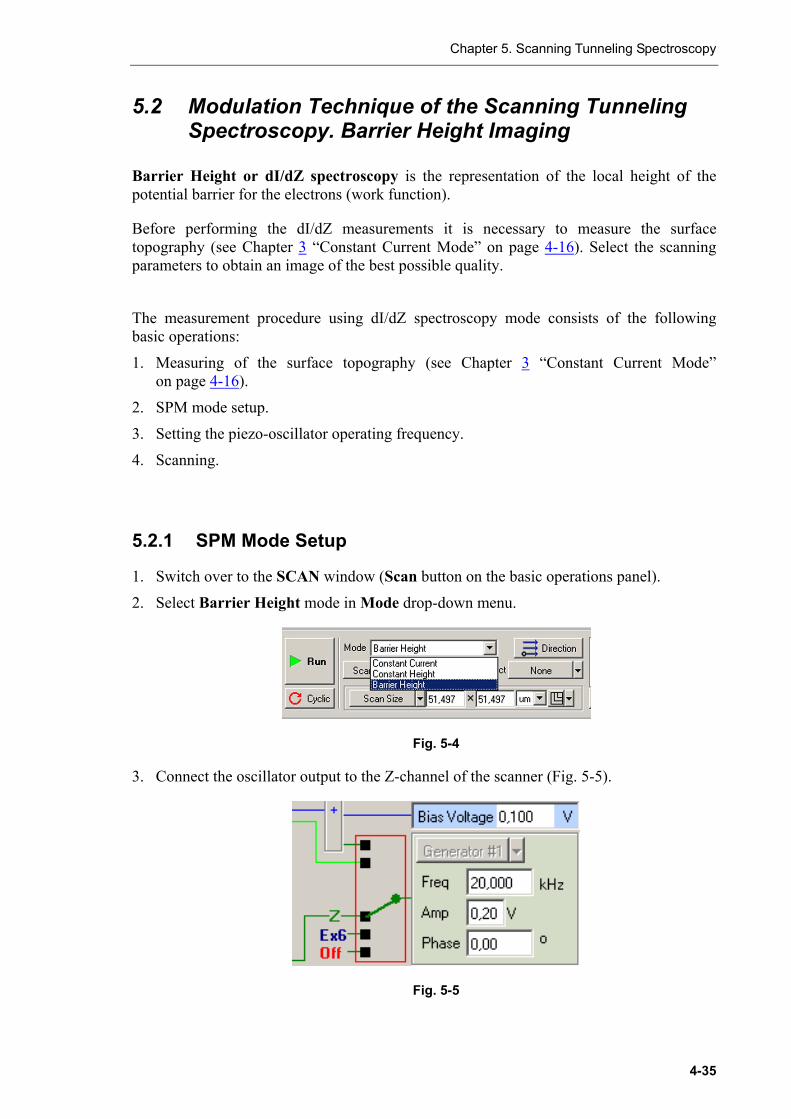
2. Select Barrier Height mode in Mode drop-down menu.

Fig. 5-4

3. Connect the oscillator output to the Z-channel of the scanner (Fig. 5-5).

Fig. 5-5

4-35

PART 4. Scanning Tunneling Microscopy

4. In the Scan Setup dialog window (click to open it) choose Mag and Height as forward signals (signal Mag is proportional to local height of potential barrier).

Fig. 5-6

5. Switch the synchronous detector input terminal to measure current. To do this:

a. Open the Additional Window by clicking on the button in the right upper corner of the control program window;

b. Open the instrument circuitry (the Scheme tab);

c. Set the synchronous detector input terminal switch to Ipr position (Fig. 5-7).

Fig. 5-7

5.2.2 Setting the Piezo-oscillator Operating Frequency

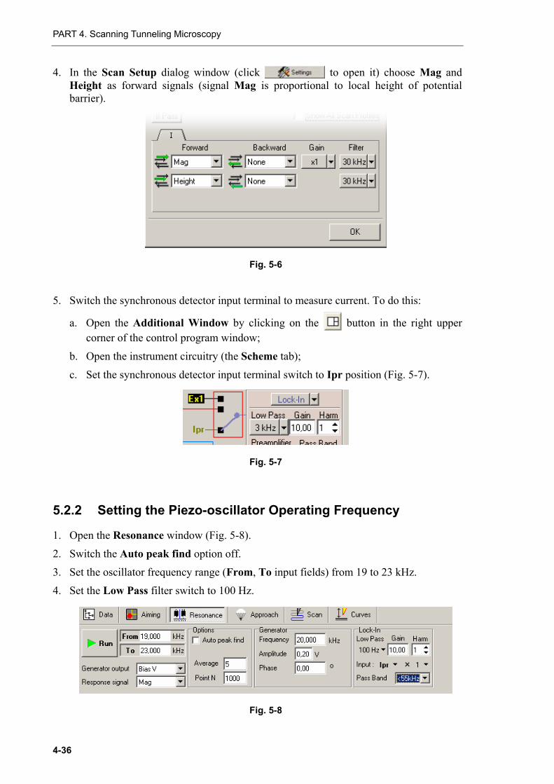
1. Open the Resonance window (Fig. 5-8).

2. Switch the Auto peak find option off.

3. Set the oscillator frequency range (From, To input fields) from 19 to 23 kHz.

4. Set the Low Pass filter switch to 100 Hz.

Fig. 5-8

4-36

Chapter 5. Scanning Tunneling Spectroscopy

5. Click the Run button.

The resonance curve of the shape, shown on Fig. 5-9 will be displayed in the oscilloscope window.

Fig. 5-9

6. Set the oscillator frequency to any of the peaks.

7. Changing the oscillator voltage (the Amplitude parameter) and observing the Mag signal change on the oscilloscope in Additional Window, set the measured Mag signal value to 2-5 nA (Fig. 5-10).

Fig. 5-10

If at the maximum value of the Amplitude parameter the Mag signal is less than 2-5 nA, then it is possible to amplify the signal being measured by modifying the Gain parameter of the synchronous detector.

4-37

PART 4. Scanning Tunneling Microscopy

5.2.3 Scanning

1. Switch over to the Scan window (Scan tab on the basic operations tabs panel).

2. Click the Run button to start scanning.

It is worth noting that the value of the measured dI/dZ signal is determined not only by the local height of the potential barrier, but also by the local hardness of the sample. For relatively “soft” samples the change of dZeff tunnel clearance value is less than dZ value of the drift of the apex of the tip, which has a pronounced effect at closer distances.

The simultaneously obtained images of the pyrolitic graphite surface (the Height window) and the change of Mag signal, proportional to the value of the Barrier Height are shown on Fig. 5-11.

Fig. 5-11. Pyrolitic graphite surface image (left) and Mag signal change (right)

4-38