Part 12: Advanced Topics in Collaborative

Filtering

Francesco Ricci

2

Content

p  Generating recommendations in CF using frequency of ratings

p  Role of neighborhood size p  Comparison of CF with association rules (“traditional”

data-mining) p  Classification and regression learning p  Memory-based CF vs. Model-Based CF p  Reliability of the user-to-user similarity p  Evaluating the importance of each rating in user-to-

user similarity p  Computational complexity of collaborative filtering.

3

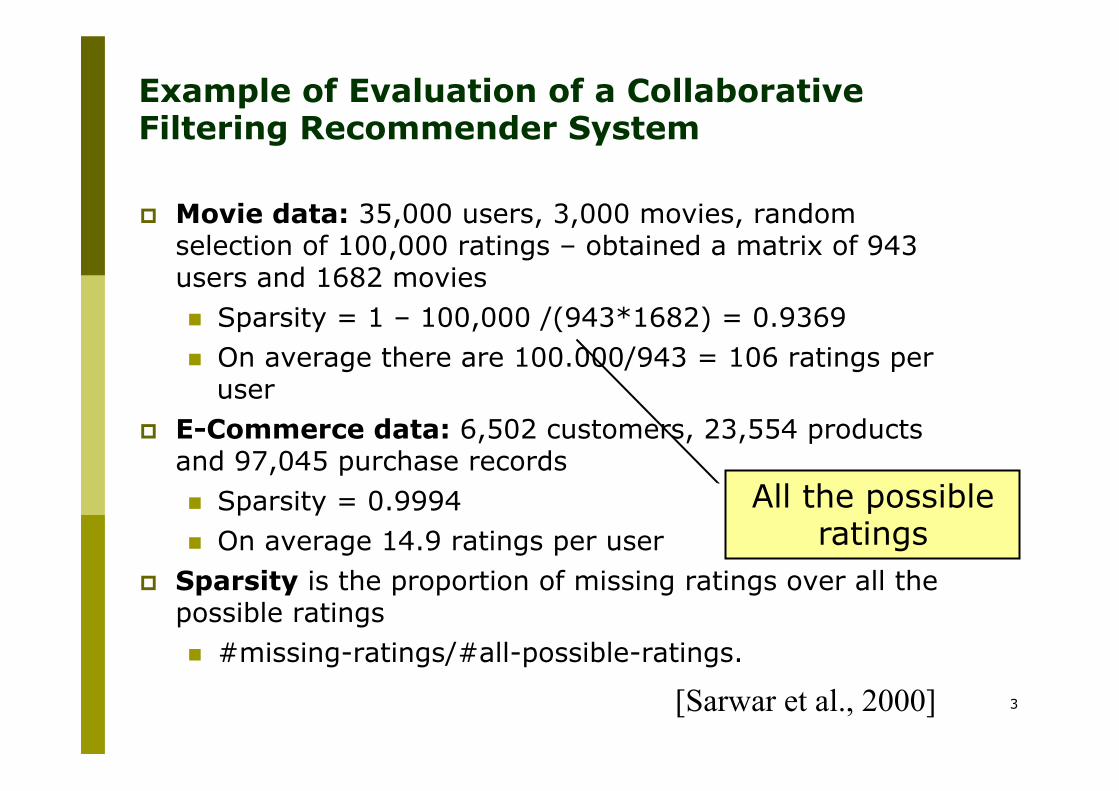
Example of Evaluation of a Collaborative Filtering Recommender System

p  Movie data: 35,000 users, 3,000 movies, random selection of 100,000 ratings – obtained a matrix of 943 users and 1682 movies n  Sparsity = 1 – 100,000 /(943*1682) = 0.9369 n  On average there are 100.000/943 = 106 ratings per

user p  E-Commerce data: 6,502 customers, 23,554 products

and 97,045 purchase records n  Sparsity = 0.9994 n  On average 14.9 ratings per user

p  Sparsity is the proportion of missing ratings over all the possible ratings n  #missing-ratings/#all-possible-ratings.

[Sarwar et al., 2000]

All the possible ratings

4

94% sparsity 99,9% sparsity

Sparsity: visual example A set of known ratings

5

Evaluation Procedure

p  They evaluate top-N recommendation (10 recommendations for each user)

p  Separate ratings in training and test sets (80% Train - 20% Test)

p  Use the training to compute the prediction (top-N) p  Compare (precision and recall) the items in the test set

of a user with the top N recommendations for that user p  Hit set is the intersection of the top N with the test set

(selected-relevant) p  Precision = size of the hit set / size of the top-N set p  Recall = size of the hit set / size of the test set p  They assume that all the rated items are relevant p  They used the cosine metric to find the neighbors.

6

Generation of recommendations p  Instead of using the weighted average of the ratings

p  They used the most-frequent item recommendation method n  Looks in the neighbors (users similar to the target

user) scanning the purchase data n  Compute the user frequency of the products in the

neighbors purchases - not already in the (training part of the) profile of the target user

n  Sort the products according to the frequency n  Returns the N most frequent products.

p  Most-frequent item recommendation computes a recommendation list without computing any rating estimation.

ruj* = ru +K wuv (rvj − rv )v∈N j (u)

∑

7

train test

Prediction for this user ?

Assume that all the depicted users are neighbors of the first one

0 Frequency of

product in neighbors purchases data

(training) 2 1 2 1 3 2

Top-4 recommended

P=2/4

R=2/3

8

Neighbor Sensitivity

EC = eCommerce data; ML = MovieLens data

Splitting the entire data set into 80% train and 20% test

Top 10 recommendations

EC users rated 14.9 items (avg) – ML users rated 106 items (avg)

Why F1 is so small? What is the maximum precision and

recall for each user in these datasets?

9

Clusters of users with 2 ratings

p  Fixed similarity threshold in two different points (users) may mean completely different neighbors

4 nearest neighbors

4 nearest neighbors

0 nearest neighbors

Movie1's rating

Mov

ie2'

s r

atin

g

10

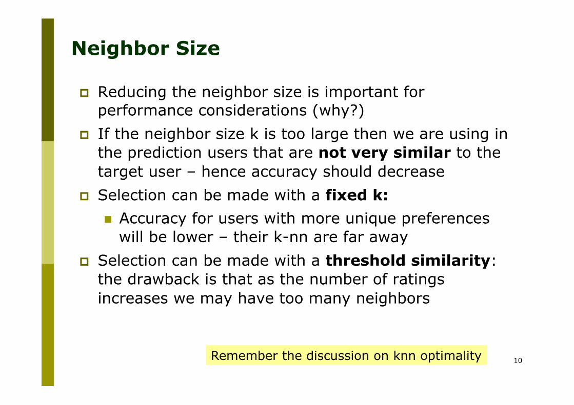
Neighbor Size

p  Reducing the neighbor size is important for performance considerations (why?)

p  If the neighbor size k is too large then we are using in the prediction users that are not very similar to the target user – hence accuracy should decrease

p  Selection can be made with a fixed k: n  Accuracy for users with more unique preferences

will be lower – their k-nn are far away p  Selection can be made with a threshold similarity:

the drawback is that as the number of ratings increases we may have too many neighbors

Remember the discussion on knn optimality

11

Neighbor Size (II)

p  When using Pearson correlation it is common to discard neighbors with negative similarity

p  Advanced techniques use “adaptive” neighbor formation algorithm – the size depends on the global data characteristics and the user and item specific ratings.

12

Association Rules

p  Discovering association between sets of co-purchased products – the presence of a set of products “implies” the presence of others

p  {p1, …, pm} = P are products, and a transaction T is a subset of products P

p  Association rule: X à Y p  X,Y are not overlapping subsets of P p  The meaning of X à Y is that in a collection of

transactions Tj (j=1, …N), if X are present it is likely that Y are also present

p  We may generate a transaction for each user in the CF system: contains the products that have been rated/purchased by the user.

13

Transactions and Ratings

0 Not Bought

1 Like or Dislike

1

0 1 1 0 1 1 0 1 1 1 1 0

Current User Users=Transactions Item

s

1st item

14th item

In [Sarwar et al., 2000] a transaction is made of all the products bought/rated by a user - not exploiting the rating values.

0

What is the

rationale?

16

Example - X à Y

p  Support = proportion of transactions that contains X and Y = 3/6

p  Confidence = proportion of those that contains X and Y over those containing X=3/4

Users=Transactions Item

s

Y

X

20

Association Rules and Recommender

p  Long term user profile: a transaction for each user containing all the products both in the past

p  Short term user profile: a transaction for each bundle of products bought during a shopping experience (e.g. a travel)

1.  Build a set of association rule (e.g. with the "Apriori" algorithm) with at least a minimum confidence and support l  [Sarwar et al., 2000] used all the users-transactions to

build the association rules l  You may use only the users close to the target (kind of

mix between AR and CF) 2.  Find the rules R supported by a user profile: X is in the

training part of the user profile 3.  Rank a product in the right-hand-side of some rules in R

with the (maximal) confidence of the rules that predict it 4.  Select the top-N

[Sarwar et al., 2000]

21

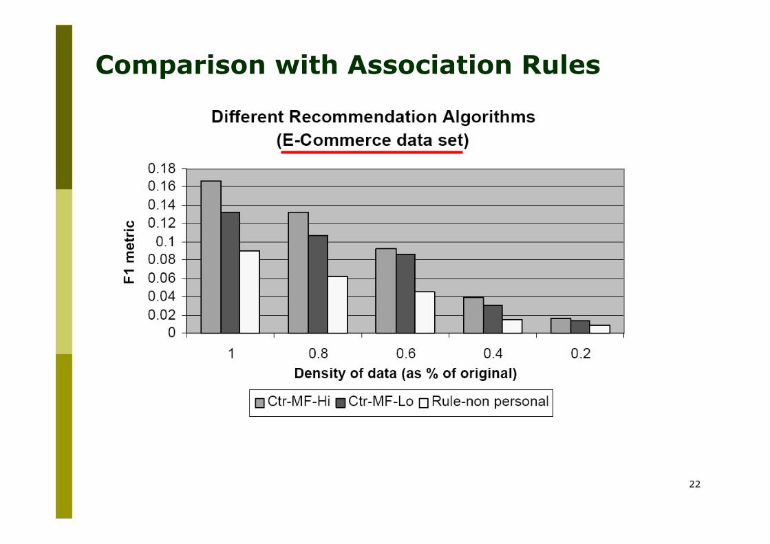
Comparison with Association Rules

“Lo” and “Hi” means low (=20) and original dimensionality for the products dimension achieved with LSI (Latent Semantic Indexing)

When we do not have enough data personalization is not useful – all these

methods tend to perform similarly

22

Comparison with Association Rules

“Lo” and “Hi” means low (=20) and original dimensionality for the products dimension achieved with LSI (Latent Semantic Indexing)

23

Classification Learning outlook temperature humidity windy Play/CLASS sunny 85 85 FALSE no

sunny 80 90 TRUE no

overcast 83 86 FALSE yes

rainy 70 96 FALSE yes

rainy 68 80 FALSE yes

rainy 65 70 TRUE no

overcast 64 65 TRUE yes

sunny 72 95 FALSE no

sunny 69 70 FALSE yes

rainy 75 80 FALSE yes

sunny 75 70 TRUE yes

overcast 72 90 TRUE yes

overcast 81 75 FALSE yes

rainy 71 91 TRUE ?

Set of classified examples

Given a set of examples for which we know the class predict the class for an unclassified examples.

24

Regression Learning outlook temperature humidity windy Play duration sunny 85 85 FALSE 5

sunny 80 90 TRUE 0

overcast 83 86 FALSE 55

rainy 70 96 FALSE 40

rainy 68 80 FALSE 65

rainy 65 70 TRUE 45

overcast 64 65 TRUE 60

sunny 72 95 FALSE 0

sunny 69 70 FALSE 70

rainy 75 80 FALSE 45

sunny 75 70 TRUE 50

overcast 72 90 TRUE 55

overcast 81 75 FALSE 75

rainy 71 91 TRUE ?

Set of examples - target feature is numeric

Given a set of examples for which we know the target (duration), predict it for examples where it is unknown.

25

Learning

p  In order to predict the class several Machine Learning techniques can be used, e.g.: n  Naïve Bayes n  K-nn n  Perceptron n  Neural Network n  Decision Trees (ID3) n  Classification Rules (AC4.5) n  Support Vector Machine

26

Items

Users

Matrix of ratings

27

Recommendation and Classification

p  Users = instances described by their ratings p  Class = the rating given by the users/instances to a target

product p  Or items=instances and class = the rating to the items/

instances given by a target user p  Differences with classical ML problems

n  Data are sparse n  There is no preferred class/item-rating to predict n  In fact, the main problem is related to determining

the classes (item ratings) that it is better to predict

n  You cannot (?) predict all and then choose the item with higher predicted ratings (too expensive)

n  Unless there are few items (? Generalize the notion of item ?).

28

Lazy and Eager Learning

p  Lazy: wait for query before generalizing n  k-Nearest Neighbor, Case based reasoning

p  Eager: generalize, i.e., build a model, before seeing query n Radial basis function networks, ID3, Neural

Networks, Naïve Bayes, SVM p  Does it matter?

n  Eager learner must create global approximation

n  Lazy learner can create many local approximations

29

Model-Based Collaborative Filtering p  Previously seen approach is called lazy or memory-based

as the original examples (vectors of user ratings) are used when a prediction is required (no computation when data is collected)

p  Model based approaches build and store a (probabilistic) model and use it to make the prediction:

p  Where r=1, …5 are the possible values of the rating and Iu is the set of items rated by user u

p  E[X] is the Expectation (i.e., the average value of the random variable X)

p  The probabilities above are estimated with a classifier producing the probability for an example to belong to a class (the class of products having a rating = r), e.g., Naïve Bayes (but also k-nearest neighbor!).

ruj* = E[ruj ]= r ∗P(ruj = r | {ruk,k ∈ Iu})

r=1

5

∑ User model

30

Naïve Bayes

p  P(H|E) = P(H) *[P(E|H) / P(E)] p  Example:

n  P(flue | fever) = P (flue) * [P(fever | flue) / P(fever)] n  P(flue | fever) = P(flue) * [0.99 / 0.03] = 0.01 * 33=

0.33 p  A class variable is the rating for a particular item (e.g., the

first item): Xi is a variable (feature) representing the rating for product i

p  Assuming the independence of the ratings on different

products

P(X1 = r | X2 = ru2,…,Xn = run ) =P(X2 = ru2,…,Xn = run | X1 = r)P(X1 = r)

P(X2 = ru2,…,Xn = run )

P(X1 = r | X2 = ru2,…,Xn = run ) =P(Xj = ruj | X1 = r)

j=2

n

∏ P(X1 = r)

P(X2 = ru2,…,Xn = run )

31

Problems of CF : Sparsity

p  Typically we have large product sets and user ratings for a small percentage of them

p  Example Amazon: millions of books and a user may have bought hundreds of them: n  The probability that two users, who have rated 100

books, have at least a common rated book (in a catalogue of 1 million books) is ~0.01 (with 50 ratings and 10 millions books is 0.00025) – if all books are equally likely to be bought!

n  Exercise: what is the probability that they have 10 books in common (stattrek.com/Tables/Binomial.aspx)

p  Hence, if you have not a large set of users it may be difficult to find out a single neighbor for a target user

p  But if there are 10,000,000 users then one can easily find 107* 0.00025 = 2,500 neighbors!

32

Reliability of the similarity measure

2

6

4 5

5

4

Overlapping ratings w

ith u1

u1

Means that there is a rating for that user-item pair

i1 i2 i3 ...

Significance of User-to-User Similarity

p  Rating data are typically sparse – user-to-user similarity weights are often computed on few ratings given to common items: Iuv

p  Take into account the significance of the user-to-user similarity metric: how dependable the measure of similarity is – and not only its value – when making a rating prediction [Herlocker et al., 1999]

p  γ is a parameter that must be cross validated – 50 gave optimal results (movielens) n  This approach improves the prediction accuracy

(MAE) 33

!wuv =min Iuv ,γ{ }

γ×wuv

35

Low variance vs. High variance items

4

6

4 5

5

4

Overlapping ratings w

ith u1

u1

5

5

5 5

5

5

5

1

2

3

4

36

Improvements of CF

p  Not all items may be informative in the similarity computation – items that have low variance in their ratings are supposed to be less informative than items that have more diverse ratings [Herlocker et al., 1999]

p  He gave more importance, in the similarity computation, to the products having larger variance in ratings – this did not improve accuracy of the prediction

p  [Baltrunas & Ricci, 2008] found good results using in the similarity computation only the most important items (feature selection: items with the highest Pearson correlation with the target item).

Inverse User Frequency

p  Items rated by a small number of users may be more informative – similar idea to "terms present in a small number of documents are more informative"

p  λi = log (|U|/|Ui|), Ui is the set of users that rated item i (assume that Ui is not empty)

p  Frequency-Weighted Pearson Correlation similarity metric:

p  [Breese et al., 1998] found that this improves prediction accuracy. 37

FWPC(u,w) =λi (rui − ru )(rvi − rv )

i∈Iuv

∑

λi (rui − ru )2 λi (rvi − rv )

2

i∈Iuv

∑i∈Iuv

∑

42

Item Popularity

3

6

5 5

3

4

u1

Popular Items

Not popular Item

43

Popular vs Not Popular

p  Predicting the rating of popular items is easier than for not popular ones: n  The prediction can be based on the ratings of

many neighbor users p  The usefulness of predicting the rating of popular

items is questionable: n  It could be guessed in a simpler way n  The system will not appear as much smart to the

user p  Predicting the rating of unpopular items is

n  Risky - not many neighbors on which to base the prediction

n  But could really bring a lot of value to the user!

44

Problems of CF : Scalability

p  Nearest neighbor algorithms require computations that grows with both the number of customers and products

p  With millions of customers and products a web-based recommender will suffer serious scalability problems

p  The worst case complexity is O(m*n) (m customers and n products)

p  But in practice the complexity is O(m + n) since for each customer only a small number of products are in the user profile and are considered for computing the similarity n  Then one loop on the m customers to compute

similarity PLUS one on the n products to compute the prediction.

45

Computational Issues

u1

To compute the similarity of u1 with the other users we must scan the users database m (large) but only 3 products will be considered (in this example)

Represent a user as u1 = ((1, r1 1), (6, r1 6), (12, r1 12))

46

Computational Issues

u1

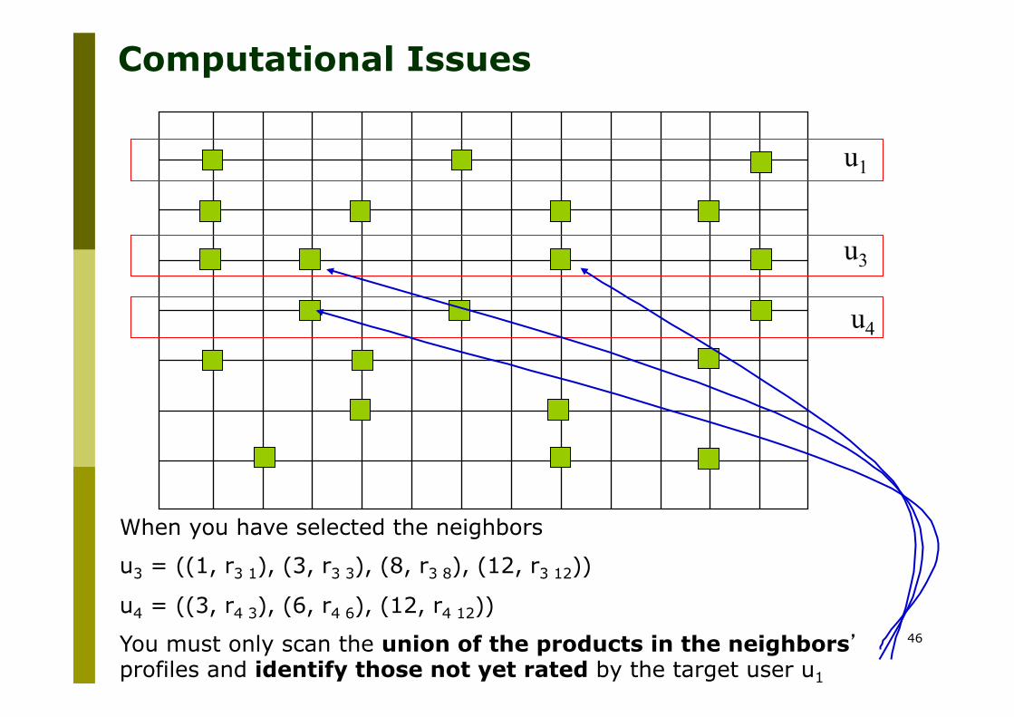
When you have selected the neighbors

u3 = ((1, r3 1), (3, r3 3), (8, r3 8), (12, r3 12))

u4 = ((3, r4 3), (6, r4 6), (12, r4 12))

You must only scan the union of the products in the neighbors’ profiles and identify those not yet rated by the target user u1

u3

u4

47

Some Solutions for Addressing the Computational Complexity

p  Discard customers with few purchases p  Discard very popular items p  Partition the products into categories p  Dimensionality reduction (LSI or clustering data) p  All of these methods also reduce

recommendation quality (according to [Linden et al., 2003]).

[Linden et al., 2003]

48

Summary

p  Example of usage of precision and recall in the evaluation of a CF system

p  CF using only the presence or absence of a rating p  Association rules p  Comparison between CF and association rules p  Illustrated the relationships between CF and

classification learning p  Briefly discussed the notion of model-based CF p  Naïve Bayes methods p  Discussed some problems of CF recommendation:

sparsity and scalability p  Discussed the computational complexity of CF

49

Questions

p  What are the two alternative approaches for selecting the nearest neighbors, given a user-to-user similarity metric?

p  How could be defined a measure of reliability of the similarity between two users?

p  What is the computational complexity of a naïve implementation of the CF algorithm? What is its complexity in practice?

p  How CF compares with association rules? p  What are the main differences between the

recommendation learning and classification learning? p  How CF would work with very popular or very rare

products? p  Will CF work better for popular or not popular items?