part 1: background in geospatial data modeling

Part 1:

Background in geospatial data

modeling

ESWC 2015 Tutorial

Publishing and Interlinking Linked Geospatial Data

Dept. of Informatics and TelecommunicationsNational and Kapodistrian University of Athens

ESWC 2015 Tutorial 2

Outline

• Basic GIS concepts and terminology

• Representing geometries

• Representing topological information

• Geospatial data standards


Basic GIS Concepts and Terminology

• Theme: the information corresponding to a particular domain

that we want to model. A theme is a set of geographic

features.

• Example: the countries of Europe


Basic GIS Concepts (cont’d)

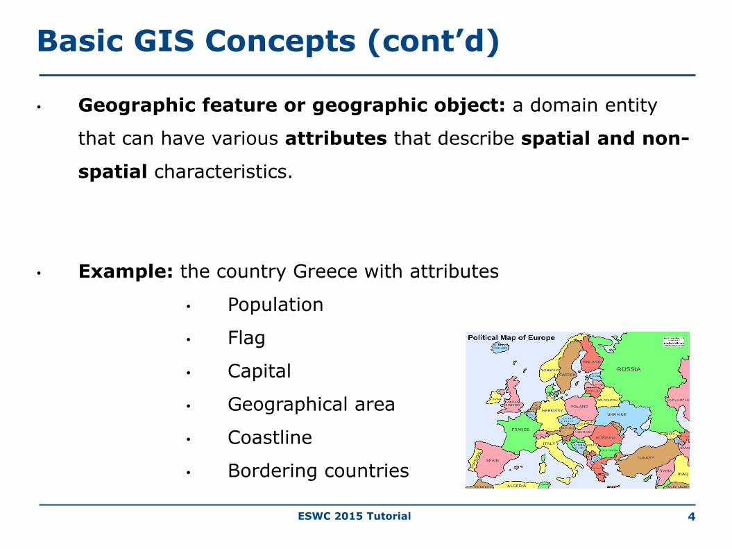
• Geographic feature or geographic object: a domain entity

that can have various attributes that describe spatial and non-

spatial characteristics.

• Example: the country Greece with attributes

• Population

• Flag

• Capital

• Geographical area

• Coastline

• Bordering countries



• Geographic features can be atomic or complex.

• Example: According to the Kallikratis administrative reform of

2010, Greece consists of:

• 13 regions (e.g., Crete)

• Each region consists of regional units (e.g., Heraklion)

• Each regional unit consists of municipalities (e.g.,

Dimos Chersonisou)

• …



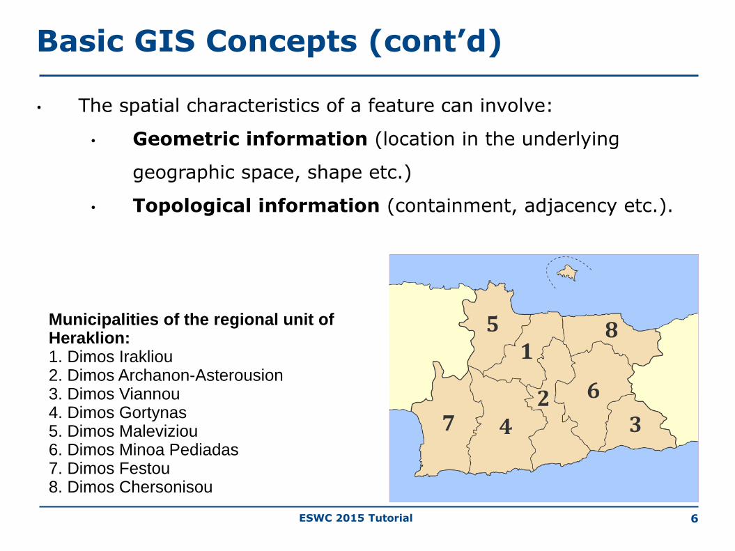
• The spatial characteristics of a feature can involve:

• Geometric information (location in the underlying

geographic space, shape etc.)

• Topological information (containment, adjacency etc.).

Municipalities of the regional unit of Heraklion:1. Dimos Irakliou2. Dimos Archanon-Asterousion3. Dimos Viannou4. Dimos Gortynas5. Dimos Maleviziou6. Dimos Minoa Pediadas7. Dimos Festou8. Dimos Chersonisou


Geometric Information

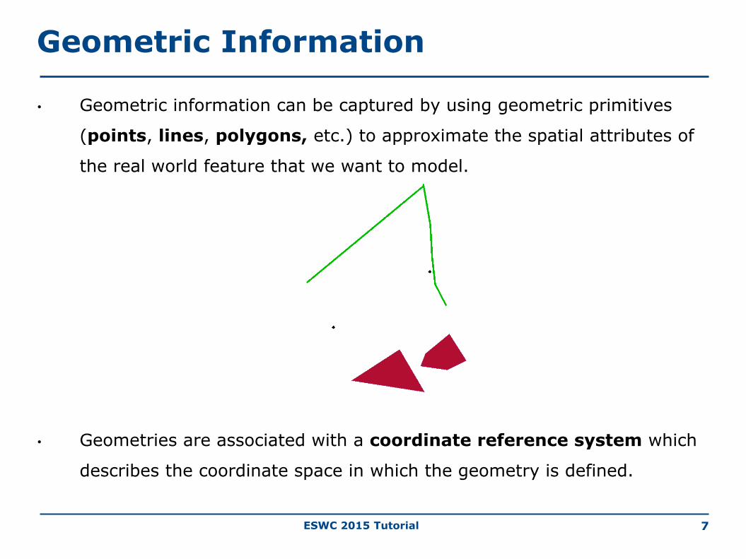
• Geometric information can be captured by using geometric primitives

(points, lines, polygons, etc.) to approximate the spatial attributes of

the real world feature that we want to model.

• Geometries are associated with a coordinate reference system which

describes the coordinate space in which the geometry is defined.


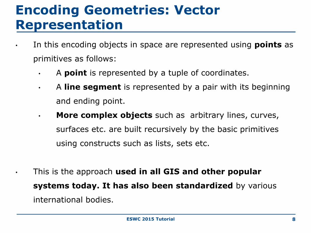
Encoding Geometries: Vector Representation

• In this encoding objects in space are represented using points as

primitives as follows:

• A point is represented by a tuple of coordinates.

• A line segment is represented by a pair with its beginning

and ending point.

• More complex objects such as arbitrary lines, curves,

surfaces etc. are built recursively by the basic primitives

using constructs such as lists, sets etc.

• This is the approach used in all GIS and other popular

systems today. It has also been standardized by various

international bodies.


Example

[(1,2) (2,2) (5,3) (3,1) (2,1) (1,2)]


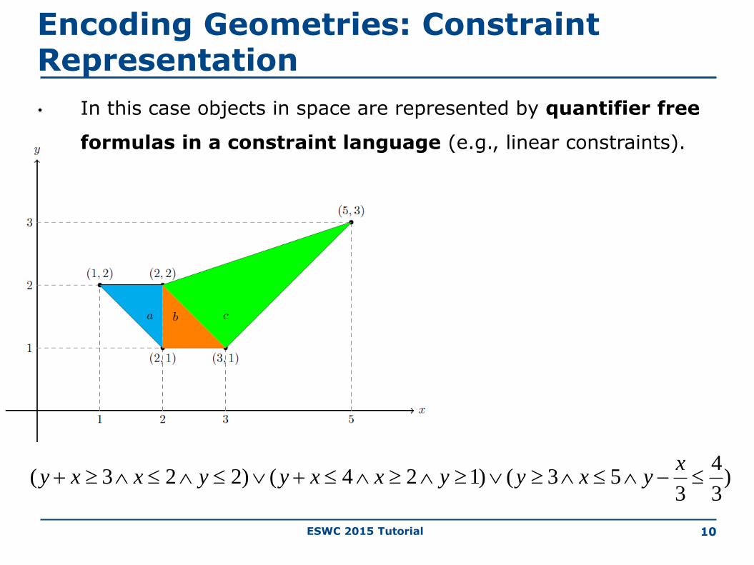
Encoding Geometries: Constraint Representation

• In this case objects in space are represented by quantifier free

formulas in a constraint language (e.g., linear constraints).

)3

4

353()124()223(

xyxyyxxyyxxy


Constraint Databases

• The constraint representation of spatial data was the focus of

much work in databases, logic programming and AI after the

paper by Kanellakis, Kuper and Revesz (PODS, 1991).

• The approach was very fruitful theoretically but was not adopted

in practice.


Topological Information

• Topological information is inherently qualitative and it is

expressed in terms of topological relations (e.g., containment,

adjacency, overlap etc.).

• Topological information can be derived from geometric

information or it might be captured by asserting explicitly the

topological relations between features.


Topological Relations

• The study of topological relations has produced

a lot of interesting results by researchers in:

• GIS

• Spatial databases

• Artificial Intelligence (qualitative reasoning

and knowledge representation)


DE-9IM

• The dimensionally extended 9-intersection model

(DE-9IM) of Clementini and Felice.

• It is based on the point-set topology of R2.

• It deals with simple, closed and connected

geometries (areas, lines, points).

• It is an extension of earlier approaches: the 4-

intersection (4IM) and 9-intersection (9IM)

models by Egenhofer and colleagues.


Topological Relations in DE-9IM

• It captures topological relationships between two

geometries a and b in R2 by considering the

dimensions of the intersections of the

boundaries, interiors and exteriors of the two

geometries:

• The dimension can be 2, 1, 0 and -1 (dimension of

the empty set).


Example

I(C) B(C) E(C)

I(A) -1 -1 2

B(A) -1 -1 1

E(A) 2 1 2

A

C


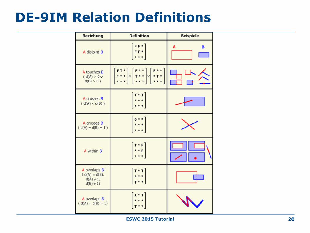
Topological Relations in DE-9IM

• The following five named relationships between two different

geometries can be distinguished: disjoint, touches, crosses,

within and overlaps.

• The named relationships have a reasonably intuitive meaning

for users. They are jointly exclusive and pairwise disjoint

(JEPD).

• The model can also be defined using an appropriate calculus of

geometries that uses these 5 binary relations and boundary

operators.


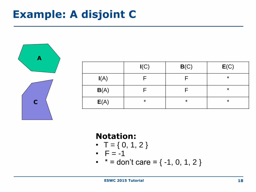
Example: A disjoint C

I(C) B(C) E(C)

I(A) F F *

B(A) F F *

E(A) * * *

A

C

Notation: • T = { 0, 1, 2 }• F = -1 • * = don’t care = { -1, 0, 1, 2 }


Example: A within C

I(C) B(C) E(C)

I(A) T * F

B(A) * * F

E(A) * * *

C

A

Notation equivalent to 3x3 matrix:

• String of 9 characters representing the above matrix in row major order.

• In this case: T*F**F***


DE-9IM Relation Definitions


The Region Connection Calculus (RCC)

• The primitives of the calculus are spatial regions. These are

non-empty, regular closed subsets of a topological space.

• The calculus is based on a single binary predicate C that

formalizes the “connectedness” relation.

• C(a,b) is true when the closure of a is connected to the

closure of b i.e., they have at least one point in common.

• It is axiomatized using first order logic.


RCC-8

• This is a set of eight JEPD binary relations that can

be defined in terms of predicate C.


RCC-5

• The RCC-5 subset has also been studied. The

granularity here is coarser. The boundary of a region is

not taken into consideration:

• No distinction among DC and EC, called just DR.

• No distinction among TPP and NTPP, called just

PP.

• RCC-8 and RCC-5 relations can also be defined

using point-set topology, and there are very close

connections to the models of Egenhofer and others.


More Qualitative Spatial Relations

• Orientation/Cardinal directions (left of, right of,

north of, south of, northeast of etc.)

• Distance (close to, far from etc.). This information

can also be quantitative.


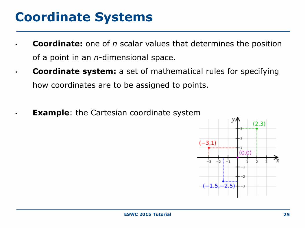
Coordinate Systems

• Coordinate: one of n scalar values that determines the position

of a point in an n-dimensional space.

• Coordinate system: a set of mathematical rules for specifying

how coordinates are to be assigned to points.

• Example: the Cartesian coordinate system


Coordinate Reference Systems

• Coordinate reference system: a coordinate system

that is related to an object (e.g., the Earth, a planar

projection of the Earth, a three dimensional

mathematical space such as R3) through a datum

which specifies its origin, scale, and orientation.

• The term spatial reference system is also used.


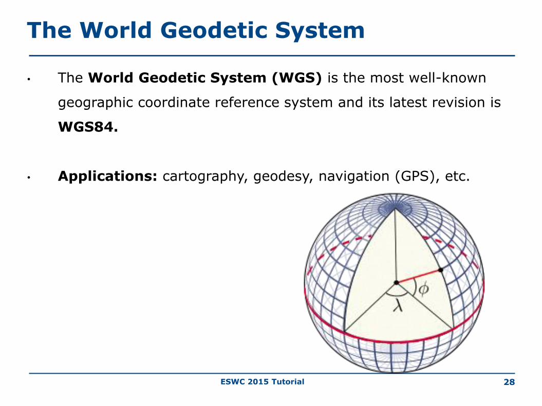
Geographic Coordinate Reference Systems

• These are 3-dimensional coordinate systems that utilize latitude

(φ), longitude (λ) , and optionally geodetic height (i.e.,

elevation), to capture geographic locations on Earth.


The World Geodetic System

• The World Geodetic System (WGS) is the most well-known

geographic coordinate reference system and its latest revision is

WGS84.

• Applications: cartography, geodesy, navigation (GPS), etc.


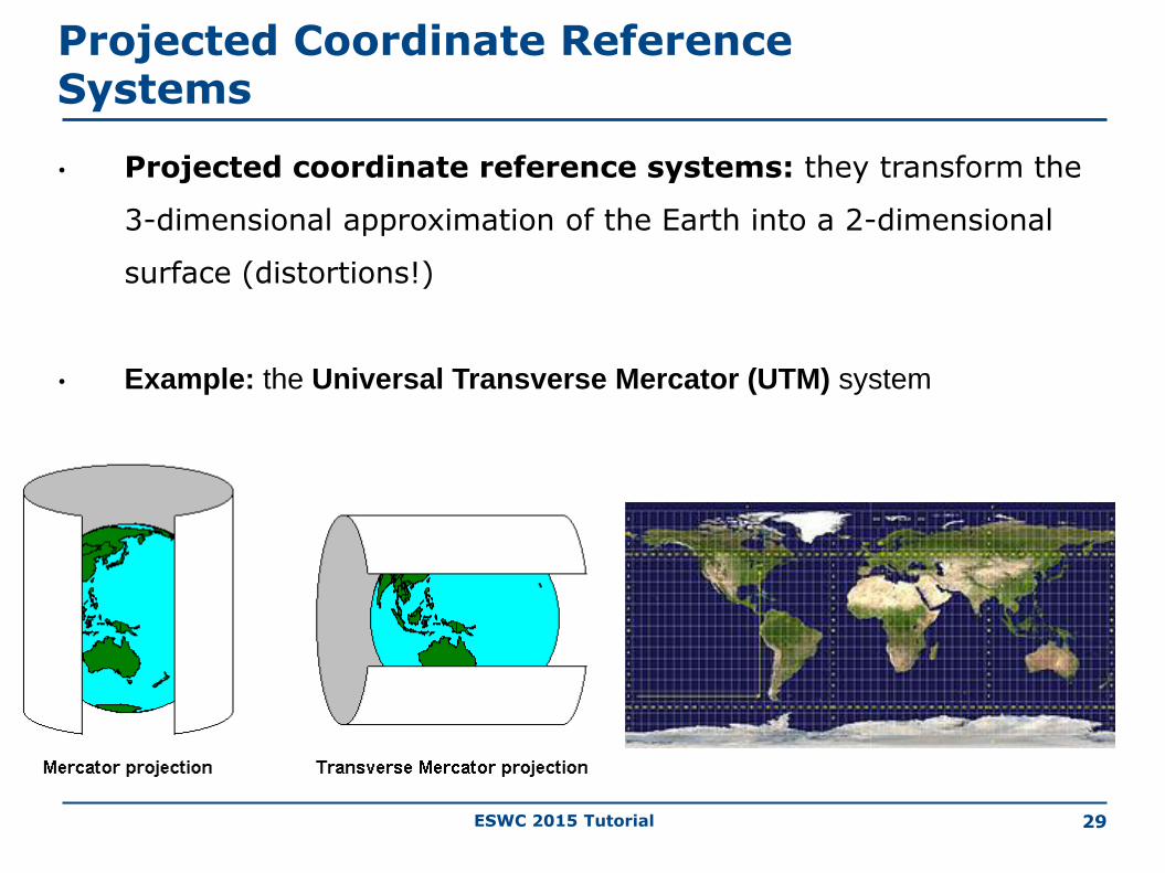
Projected Coordinate Reference Systems

• Projected coordinate reference systems: they transform the

3-dimensional approximation of the Earth into a 2-dimensional

surface (distortions!)

• Example: the Universal Transverse Mercator (UTM) system


Coordinate Reference Systems (cont’d)

• There are well-known ways to translate between co-

ordinate reference systems.

• See the list of coordinate reference systems of the

European Petroleum Survey Group: http://www.epsg-

registry.org/

http://www.epsg-registry.org/


Geospatial Data Standards

• The Open Geospatial Consortium (OGC) and the

International Organization for Standardization (ISO) have

developed many geospatial data standards that are in wide use

today. In this tutorial we will cover:

• Well-Known Text

• Geography Markup Language

• OpenGIS Simple Features Access


Well-Known Text (WKT)

• WKT is an OGC and ISO standard for representing geometries,

coordinate reference systems, and transformations between

coordinate reference systems.

• WKT is specified in OpenGIS Simple Feature Access - Part 1:

Common Architecture standard which is the same as the ISO 19125-1

standard. Download from

http://portal.opengeospatial.org/files/?artifact_id=25355 .

• This standard concentrates on simple features: features with all

spatial attributes described piecewise by a straight line or a

planar interpolation between sets of points.

http://portal.opengeospatial.org/files/?artifact_id=25355


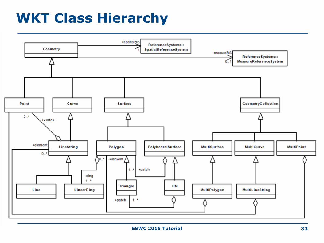
WKT Class Hierarchy


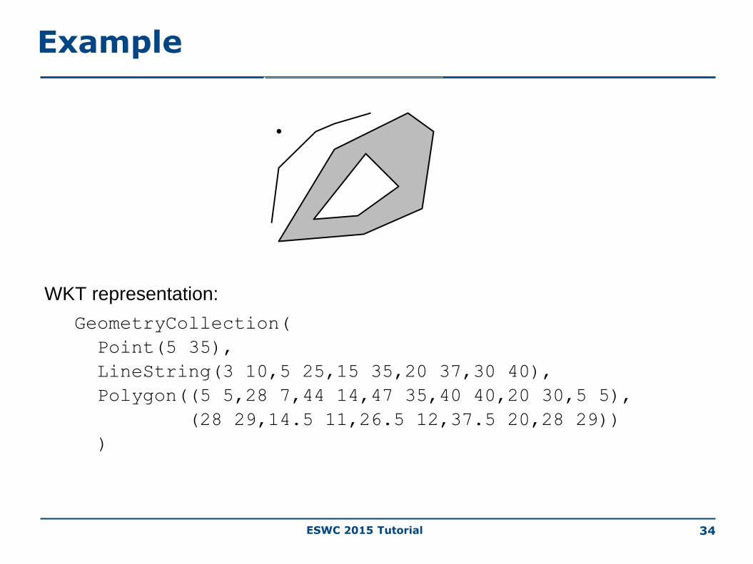
Example

WKT representation:

GeometryCollection(

Point(5 35),

LineString(3 10,5 25,15 35,20 37,30 40),

Polygon((5 5,28 7,44 14,47 35,40 40,20 30,5 5),

(28 29,14.5 11,26.5 12,37.5 20,28 29))

)


Geography Markup Language (GML)

• GML is an XML-based encoding standard for the

representation of geospatial data.

• GML provides XML schemas for defining a variety of concepts:

geographic features, geometry, coordinate reference

systems, topology, time and units of measurement.

• GML profiles are subsets of GML that target particular

applications.

• Examples: Point Profile, GML Simple Features Profile etc.


GML Simple Features: Class Hierarchy


Example

GML representation:

<gml:Polygon gml:id="p3" srsName="urn:ogc:def:crs:EPSG:6.6:4326”>

<gml:exterior>

<gml:LinearRing>

<gml:coordinates>

5,5 28,7 44,14 47,35 40,40 20,30 5,5

</gml:coordinates>

</gml:LinearRing>

</gml:exterior>

</gml:Polygon>


OpenGIS Simple Features Access

• OGC has also specified a standard for the storage, retrieval,

query and update of sets of simple features using

relational DBMS and SQL.

• This standard is “OpenGIS Simple Feature Access - Part 2: SQL

Option” and it is the same as the ISO 19125-2 standard. Download from

http://portal.opengeospatial.org/files/?artifact_id=25354.

• Related standard: ISO 13249 SQL/MM - Part 3.

http://portal.opengeospatial.org/files/?artifact_id=25354


OpenGIS Simple Features Access (cont’d)

• The standard covers two implementations options: (i) using only

the SQL predefined data types and (ii) using SQL with

geometry types.

• SQL with geometry types:

• We use the WKT geometry class hierarchy presented earlier

to define new geometric data types for SQL

• We define new SQL functions on those types.


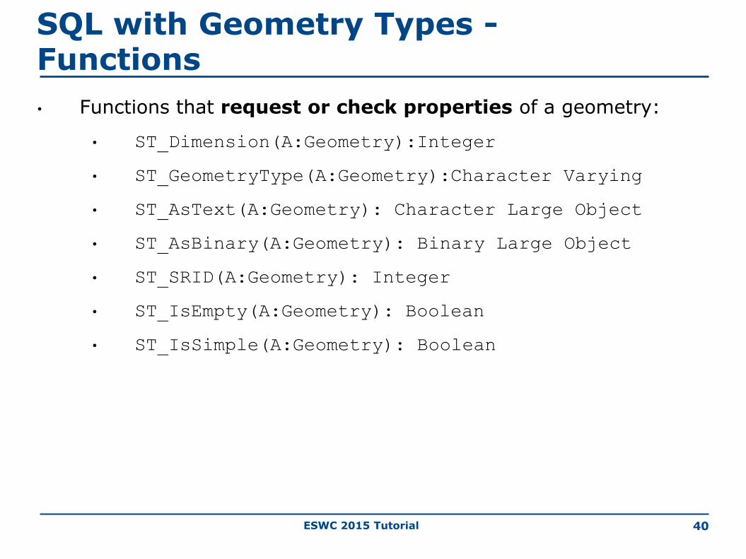
SQL with Geometry Types -Functions

• Functions that request or check properties of a geometry:

• ST_Dimension(A:Geometry):Integer

• ST_GeometryType(A:Geometry):Character Varying

• ST_AsText(A:Geometry): Character Large Object

• ST_AsBinary(A:Geometry): Binary Large Object

• ST_SRID(A:Geometry): Integer

• ST_IsEmpty(A:Geometry): Boolean

• ST_IsSimple(A:Geometry): Boolean


SQL with Geometry Types –Functions (cont’d)

• Functions that test topological relations between two geometries

using the DE-9IM:

• ST_Equals(A:Geometry, B:Geometry):Boolean

• ST_Disjoint(A:Geometry, B:Geometry):Boolean

• ST_Intersects(A:Geometry, B:Geometry):Boolean

• ST_Touches(A:Geometry, B:Geometry):Boolean

• ST_Crosses(A:Geometry, B:Geometry):Boolean

• ST_Within(A:Geometry, B:Geometry):Boolean

• ST_Contains(A:Geometry, B:Geometry):Boolean

• ST_Overlaps(A:Geometry, B:Geometry):Boolean

• ST_Relate(A:Geometry, B:Geometry, Matrix: Char(9)):Boolean


DE-9IM Relation Definitions

• A equals B can also be defined by the pattern TFFFTFFFT.

• A intersects B is the negation of A disjoint B

• A contains B is equivalent to B within A


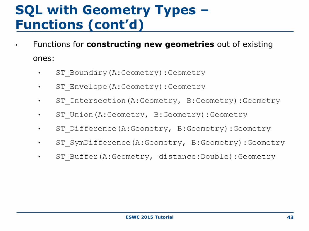
SQL with Geometry Types –Functions (cont’d)

• Functions for constructing new geometries out of existing

ones:

• ST_Boundary(A:Geometry):Geometry

• ST_Envelope(A:Geometry):Geometry

• ST_Intersection(A:Geometry, B:Geometry):Geometry

• ST_Union(A:Geometry, B:Geometry):Geometry

• ST_Difference(A:Geometry, B:Geometry):Geometry

• ST_SymDifference(A:Geometry, B:Geometry):Geometry

• ST_Buffer(A:Geometry, distance:Double):Geometry


Geospatial Relational DBMS

• The OpenGIS Simple Features Access Standard is today been

used in all relational DBMS with a geospatial extension.

• The abstract data type mechanism of the DBMS allows

the representation of all kinds of geospatial data types

supported by the standard.

• The query language (SQL) offers the functions of the

standard for querying data of these types.

• The book Geographic Information Systems and Science is a nice introduction to GIS. See: http://eu.wiley.com/WileyCDA/WileyTitle/productCd-EHEP001475.html

• The following papers present the DE-9IM model:

Eliseo Clementini, Paolino Di Felice and Peter van Oosterom.

A Small Set of Formal Topological Relationships Suitable for End-User Interaction. SSD 1993: 277-295

http://link.springer.com/chapter/10.1007%2F3-540-56869-7_16

E. Clementini and P. Felice. A Comparison of Methods for Representing Topological Relationships. Information Sciences 80 (1994), pp. 1-34.

http://www.sciencedirect.com/science/article/pii/106901159400033X The paper

• The paper below surveys a lot of interesting results on the RCC calculus:J. Renz, B. Nebel, Qualitative Spatial Reasoning using Constraint

Calculi, in: M. Aiello, I. Pratt-Hartmann and J. van Benthem (eds.),

Handbook of Spatial Logics, pp. 161–215, 2007, Springer.http://users.cecs.anu.edu.au/~jrenz/papers/renz-nebel-los.pdf

• The two OGC standards mentioned in the slides.

Readings

http://link.springer.com/chapter/10.1007/3-540-56869-7_16

http://users.cecs.anu.edu.au/~jrenz/papers/renz-nebel-los.pdf

part 1: background in geospatial data modeling

Documents