parking spaces in the age of shared autonomous …docs.trb.org/prp/17-05399.pdf102 included parking...

Zhang, Guhathakurta 1

Parking spaces in the age of shared autonomous vehicles: How 1 much parking will we need and where? 2 3 4 5 Wenwen Zhang 6 Georgia Institute of Technology: School of City & Regional Planning 7 760 Spring Street, Atlanta, GA, 30318 8 404-910-5023 9 [email protected] 10 11 Subhrajit Guhathakurta 12 Georgia Institute of Technology: School of City & Regional Planning 13 760 Spring Street, Atlanta, GA, 30318 14 404-385-0900 15 [email protected] 16 17 18 Word Count: 5,663+ 7 Figures *250 = 7,413 19 20 Revised and resubmitted: Nov. 15th, 2016 21 22


ABSTRACT 23 We are on the cusp of a new era in mobility given that the enabling technologies for 24 autonomous vehicles (AVs) are almost ready for deployment and testing. While the 25 technological frontiers for deploying AVs are being crossed, we know far less about the 26 potential impact of such technologies on urban form and land use patterns. This paper 27 attempts to address these issues by simulating the operation of Shared AVs (SAVs) in the 28 City of Atlanta, USA, using the real transportation network with calibrated link-level travel 29 speeds, and travel demand origin-destination (OD) matrix. The model results suggest the 30 SAV system can reduce parking land by 4.5% in Atlanta, at a 5% market penetration level. In 31 charged parking scenarios, parking demand will move away from downtown to adjacent low-32 income neighborhoods. The results also reveal that policymakers may consider combining 33 charged parking policies with additional regulations to curb excessive VMT and alleviate 34 potential social equity problems. 35 36 Keywords: Shared Autonomous Vehicles, Parking, Land Use, Atlanta 37 38


INTRODUCTION 39 Autonomous vehicles, cars that drive themselves, are being tested for deployment in various 40 locations around the globe. Multiple companies, including Google, Audi, Nissan, Tesla and 41 BMW, have announced plans to have fully automated cars by 2020. Indeed, the deployment 42 of small-scale, low-speed, automated mobility on demand systems will soon be tested in 43 Europe [1] and possibly by Google and Uber shortly [2,3]. Recently, the U.S. Department of 44 Transportation unveiled new policy guidance anticipating widespread deployment of AVs 45 [4]. The vehicle automation technology combined with the sharing economy will 46 undoubtedly lead to a new travel mode – Shared Autonomous Vehicles (SAVs), a centralized 47 taxi service without drivers, which will be more affordable and environmentally friendly to 48 operate than private AVs [5,6]. 49

This promising SAV system will inevitably lead to changes in the urban parking land 50 use. One Previous study, based on the simulation of SAV operations in a hypothetical grid-51 based city, revealed that the SAV may eliminate a significant amount of parking demand for 52 participating households [7]. This study adds to the proliferating literature on the impact of 53 SAVs based on real-world data-driven simulation. We developed a discrete event simulation 54 (DES) model to examine the impact of SAVs on urban parking land use at various parking 55 price settings. The model output provides insights about the amount and the spatial 56 distribution of parking for the SAV system. 57

PREVIOUS WORK 58 Although SAVs are yet to be deployed, there has been a growing literature exploring 59

different aspects of the system using simulation approaches. Several pioneering studies have 60 validated the feasibility and affordability of the SAV system. Ford [8] and Kornhauser [9] 61 evaluated the performance of a shared taxi system, aTaxi system, with fixed service stations 62 distributed every half-mile in a region and demonstrated that the system could fulfill the 63 travel demands. Burns et al. [5] developed a more advanced agent-based simulation model to 64 show that the cost per trip mile can range from $0.32 to $0.39, which is more affordable than 65 the existing private vehicles. Bridges [10] suggested electric autonomous vehicles can reduce 66 the cost to $0.13, and the SAVs can still anticipate a 30% profit margin. At this price point 67 the SAV system competes well with almost all existing public transit systems currently 68 operating in the US. Recent commercial reports also suggested that the cost of SAVs can be 69 significantly lower than conventional taxis and privately owned vehicles, ranging from 17 to 70 46 cents per mile [11-13]. 71

A handful of studies has shown that the SAV system is environmental friendly. 72 Fagnant and Kockelman's [6] study found that each SAV could replace around 11 privately 73 owned vehicles, which can lead to 12% reductions in energy consumptions, and 5.6% 74 decrease in GHG emissions per vehicle life cycle. However, the study pointed out that the 75 SAV system generates 10.7% more Vehicle Miles Travelled (VMT) due to deadhead. Such 76 side effect, nevertheless, can be alleviated via the dynamic ride-sharing techniques [14, 15]. 77 One recent study suggested despite the excessive VMT generation, electricity powered SAVs 78 can reduce GHG emissions by more than 85% [16]. 79

Some other studies built on Fagnant and Kockelman's [6] model and explored the 80 impact of SAV system on urban infrastructures. Zhang et al. [7] explored the impact of SAVs 81 on the urban parking space and found that 90% reduction could be achieved for participating 82 households. Chen, Kockelman, & Hanna [17] integrated the electric vehicle charging 83 component into the model to analyze the spatial layout of charging stations for the Shared 84 Autonomous Electric Vehicle (SAEV) system. 85

All of the mentioned studies developed models under the grid-based city setting and 86 hence are constrained by several assumptions, including grid-based transportation network, 87


constant link level travel speed across the network, and homogeneous households in the 88 hypothetical city. More recent literature overcame these limitations by simulating the 89 operation of SAV system in a real-world context. Fagnant et al. [14] implemented the SAV 90 system in Austin, TX, to determine required fleet size and examine the system performance. 91 International Transport Forum (ITF) [18] explored the impact of the system on urban traffic 92 in Lisbon and found a 35% increase in peak traffic flow and 90% reduction in parking 93 demand. Spieser et al. [19] studied the feasibility of a SAV system and the level of service 94 that the system may offer in Singapore and found that the system was capable of serving the 95 entire population. Rigole [20] simulated a SAV system that serves all the commuting trips in 96 Stockholm and identified significant reduction in air pollutant emissions from that system. 97 Shen & Lopes’s [21] simulation indicated the SAV system could outperform the existing 98 New York taxi system via a centralized operation. 99

Although the literature regarding the SAV system is flourishing, only two previous 100 studies quantified the influence of the system on urban parking land use. Zhang et al. [7] 101 included parking estimation module in the simulation to examine the overall reduction in 102 parking demand. However, the model simulates a hypothetical grid-based city with 103 undifferentiated links and nodes. Thus, the study offers limited information about parking 104 implications for a real city. While the ITF [18] study developed a SAV model for the city of 105 Lisbon, the primary objective was to explore traffic volume variations, not changes in 106 parking demand. Neither parking infrastructure availability nor parking price was considered 107 in both studies. Finally, both models used the activity scanning simulation framework, i.e. 108 time is advanced in small but constant time steps. The framework trades off simulation time 109 and time-related output resolutions. This paper breaks new ground by simulating the 110 operation of SAVs in the City of Atlanta, USA, using the real parking inventory and 111 transportation network with calibrated link-level travel speeds, travel demand origin-112 destination (OD) matrix, and synthesized travel profiles. The simulation results will provide 113 the temporal and spatial patterns of parking demand under different parking price policies. 114 Furthermore, the study implements the Discrete Event Simulation (DES) framework, which 115 has several advantages over activity scanning based SAV models developed in prior studies. 116

MODEL FORMULATION 117 Fundamentals of DES 118 The DES technique models the operation of a system as a sequence of events in time. The 119 time variable notated as !, advances when and only when an event occurs. Events are only 120 scheduled if there will be changes in the state of the system. Therefore, in DES models, the 121 simulation time jumps inconsistently from one event to the next. On the other hand, the 122 activity-scanning or time-step based models breaks the simulation up into small, constant 123 time slices and the system attempts to update the states at each time slice. Therefore, in 124 activity-scanning models, time advances by constant time-steps defined by the simulator 125 designer. In this study, the DES model presents two advantages compared with activity-126 scanning models. First, there will be no tradeoff between simulation time resolution and 127 model runtime. Second, the DES framework significantly reduces coding complexity and 128 model runtime by not simulating the micro-changes rising from the movement of busy 129 vehicles. The following sections elaborate on the conceptual model and implementation 130 algorithms for the simulator. 131 132 Model Objective and Scenarios 133 The goal of this study is to examine the impact of different parking price polices on the 134 parking footprint of the SAV system and the tradeoffs between parking fees, VMT 135 generation, and client’s average waiting time. We investigated three parking price scenarios. 136


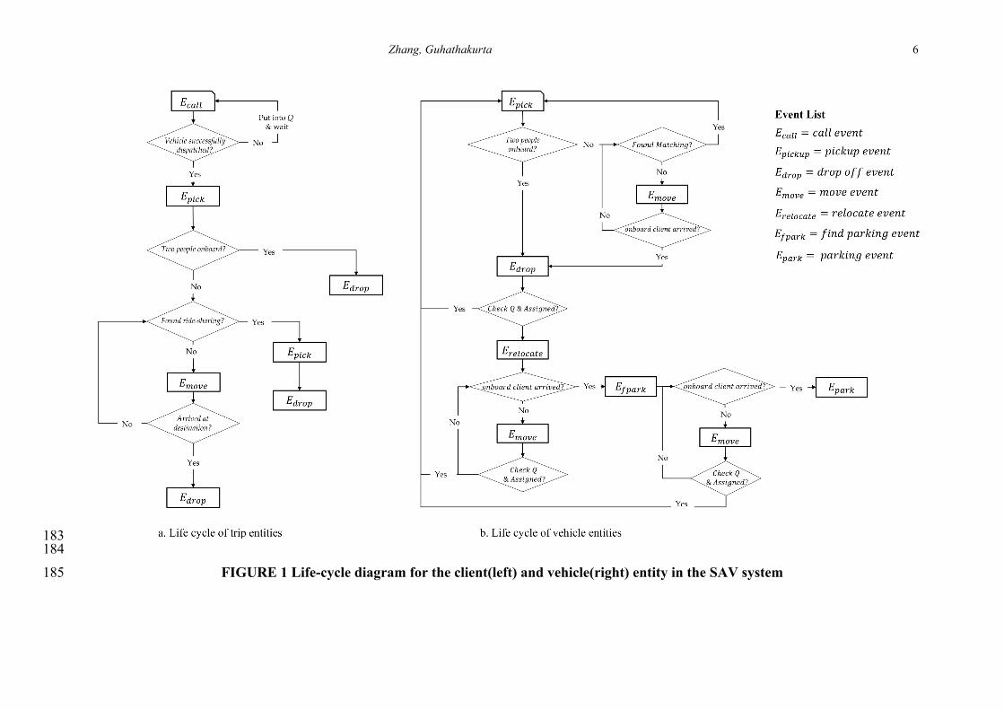
These are: 1) free parking, 2) entrance-based charged parking, and 3) time-based charged 137 parking. In the free parking scenario, the SAVs can enter all the existing parking 138 infrastructure as long as there is available space in the lot. In the entrance-based charging 139 scenario, the SAVs need to pay an entrance fee whenever they enter the parking lot, 140 regardless of the length of time parked. In the time-based parking scenario, the SAVs pay for 141 parking after leaving the parking lots based on the actual parking duration. The two charged 142 parking scenarios vary parking charges based on the variation in land values in different parts 143 of the city. 144 145 Model Entities and Activities 146 In the SAV system, there are four types of entities. These include: 1) the vehicle entity, 2) the 147 trip entity, 3) the queue entity and 4) the parking lot entity. All entities in the model will get 148 involved in a sequence of activities. For each trip entity, the model schedules a call event at 149 the trip departure time. When handling the call events, the system dispatches the vehicle with 150 the least trip cost and schedules a pickup event. If the vehicle assignment process fails, the 151 trip entity will be put on a waiting list, i.e. the queue entity. After picking up a client, the 152 vehicle either picks up a second client (if ride-sharing can be established) or schedule a drop-153 off event upon arrival at the trip destination. If a busy vehicle becomes empty, the system will 154 schedule a relocation event to balance vehicle distribution, if necessary. If a vehicle remains 155 idling after relocation (or after drop-off in case relocation was not triggered), the system 156 schedules find park event to identify a parking lot entity, which minimizes the total parking 157 cost, and eventually schedules a park event upon arrival. The move events are scheduled to 158 transfer the vehicles to another location or to a parking lot. The move events can be 159 interrupted if the moving vehicle is assigned to serve incoming trips. The life-cycle diagrams 160 in Figure 1 illustrate the sequence of events that trip and vehicle entities may go through in 161 the simulation. The design of the events will be elaborated in the following sections. 162 163 Call Event 164 At the beginning of each simulation day, the model generates trip entities based on the local 165 OD matrix and a recent travel survey. Assuming that the trip generation follows Poisson 166 Distribution [6], we simulate the total number of produced trips for each OD pair " and # by 167 generating a Poisson random number given the average trip number, $%,', from the local OD 168 matrix. 169 170

()*+,"-%' = /0123*. 53"66"31($%,') 171 172

For each generated trip 9, the trip departure time is assigned based on the formula 173 below. The Cumulative Density Function (CDF) for trip departure time is estimated based on 174 the weighted local travel survey. 175 176

:;-0,!),;+"*;< = =:>?@AB(,) 177 178 where, 179 ,, is uniformly distributed random number from 0 to 1. 180 =:>?@AB(,), is the inversed CDF for trip departure time. 181 182


183 184

FIGURE 1 Life-cycle diagram for the client(left) and vehicle(right) entity in the SAV system185


For each generated trip entity, the model schedules a call event at trip departure time 186 dt. Upon the occurrence of the call event, the system dispatches SAVs to fulfill the travel 187 demand. The system searches for SAVs whose status is not labelled as “busy” and assigns the 188 one that offers the lowest costs, including both time and fare costs to serve. 189 190

!""#$%&')!*+ = min+∈12

(4#5&67"4+ + 9:;&67"4+) 191 192 Where, 193 = is the index for vehicle; 194 >? is a set of indices for vehicles whose status is not “busy”; 195 4#5&67"4+ is the potential excessive travel time cost if jth vehicle was assigned; 196 9:;&67"4+is the anticipated fare cost if jth vehicle was assigned. 197 198

The time cost is calculated based on the assumption that the waiting time is valued as 199 half of people’s hourly wage [7]. In the ride-sharing process, the vehicle does not operate on 200 the first come first serve basis but optimize the route to minimize VMT. In return, each client 201 can benefit from 40% reduction in SAV fare. 202 203

4#5&67"4+ = 0.5CD. ":E:;F ∗ H#6I#%$JHK:#4#%$4#5&+ + '&47J;4#5&+ 204 205

9:;&67"4+ = $0.5 ∗ '&E#M&;4F4#5&+,%7;#'& − "ℎ:;#%$&"4:QE#"ℎ&'

$0.3 ∗ '&E#M&;4F4#5&+,#9;#'& − "ℎ:;#%$#"&"4:QE#"ℎ&' 206

207 Ride-sharing will only be established if the following criteria are satisfied. 208 1) The excessive time for both trips is equal or smaller than 15% of travel time without 209

ride-sharing; 210 2) For short intra-zonal trips, the acceptable maximum detour time is set as 3 minutes; 211 3) The ride-sharing induced detour time should be compensated by the decrease in SAV 212

fare for both clients. 213 214

If a vehicle is assigned, then the status of the vehicle will be updated to “busy”. A pickup 215 event will be scheduled at the estimated arrival time at the trip origin. Meanwhile, the system 216 frees up a parking space if the vehicle was parked. The trip will be put on a waiting list if the 217 system fails to arrange service. 218 219 Pickup Event 220 In the pickup event, the vehicle picks up the waiting client and then updates system states 221 based on the vehicle occupancy. If there is only one onboard client, then the status of the 222 vehicle becomes “one available”, the path will be updated to the shortest path to deliver the 223 client, and a move event will be scheduled to push vehicle towards the destination. If the 224 vehicle picks up a second ride-sharing client, then the status of the vehicle changes to “busy” 225 and the path will be updated to the shortest path to serve both clients. A drop-off event will 226 be scheduled for the client who should be dropped off first given the updated path. 227 228 Move Event 229 The system handles a move event based on the status of the vehicle. If the status of the 230 vehicle is “one available”, the system will try to find potential ride-sharing. For the other 231 types moves, such as relocating or parking vehicles, the system attempts to assign the vehicle 232 to serve the closest waiting trip. Once assigned for service, the vehicle become “busy” and a 233


pickup event will be scheduled. If the vehicle is not assigned for service and has not arrived 234 at its destination, the vehicle moves onto the next node in the network towards the 235 destination. If the vehicle has arrived at the destination, the system schedules drop-off, find 236 parking, or park event for “one available”, “relocating”, or “parking” vehicles separately. 237 238 Drop-off Event 239 In this event, the vehicle drops off the client who has arrived at the destination. After 240 dropping off the client, if the vehicle becomes empty, the status of the vehicle changes to 241 “available” and a relocation event will be scheduled. Otherwise, if there remains onboard 242 client, the system schedules another drop-off event. 243 244 Relocate Event 245 The primary goal of the relocation event for jth vehicle is to balance the spatial distribution of 246 available vehicles to reduce average waiting time. This event builds on the existing SAV 247 relocation algorithm [6] to relocate the vehicle from surplus zones to underserved areas. For 248 each zone the imbalance value is calculated using the formula below: 249 250

S5Q:E:%6&D = ()!*"D

)!*"TUVWX−

Y&5:%'D

Y&5:%'TUVWX)/

Y&5:%'D

Y&5:%'TUVWX 251

252 where, 253 i is the index for zones; 254 )!*"D/)!*"TUVWX is the share of available SAV in zone i 255 Y&5:%'D/Y&5:%'TUVWX is the share of travel demand in zone i. 256 257 If the vehicle is in a zone with imbalance value larger than 10%, then the system allocates the 258 vehicle to zone j where the imbalance value is the smallest in the service area, updates 259 relocating path, labels the vehicle as “relocating”, and schedules a move event. Otherwise, 260 the system directly schedules a find parking event. 261 262 Find Parking Event 263 In the find parking event, the status of the vehicle will be labeled as “parking”. The zone with 264 the lowest potential parking cost, calculated using the formula below, will be identified as the 265 parking destination for the vehicle. In the time-based charging scenario, the potential parking 266 cost is the product of expected parking time and the hourly parking price. The expected 267 parking time matrix is initiated using averages from free-parking scenario and is updated 268 every 10 minute. After determining the parking destination, the system updates the path for 269 the vehicle, reserves one parking space at the destination and schedules a move. 270 271

[T?\ = min]∈^2

(9J&E67"4D,] + H:;I#%$67"4]) 272

H:;I#%$67"4+ =

0, _;&&H:;I#%$"6&%:;#7

&%4;:%6&H;#6&], `%4;:%6& − Q:"&'6ℎ:;$#%$"6&%:;#7

ℎ7J;EFH;#6&] ∗ ℎ7J;],V, C#5& − Q:"&'6ℎ:;$#%$"6&%:;#7

273

274 Where, 275 # is the zone index for the current location of the vehicle; 276 I is an index from a set a? which contain all zones where parking space remain available; 277 ℎ7J;],V is the anticipated parking time at zone I and time 4. 278 279


Park Event 280 In the park event, the jth vehicle’s status will be changed to “parked”. There will be no other 281 changes to the states of the system, until the vehicle is assigned again to serve incoming calls. 282 283 Model Inputs and Outputs 284 There are several inputs for the model, including transportation infrastructures, local travel 285 demand, local income distribution, and SAV fleet size, among others, to assign values for 286 attributes of different entities. Local transportation infrastructure data provides information 287 about road network composition, link level travel speed by time of the day, and parking 288 inventory, including the number of spaces and prices. The local OD matrix, and travel survey 289 offers information regarding the trip origins, destinations and departure time. The primary 290 model outputs include the spatial and temporal patterns of parking demand, i.e., the number 291 of times that SAVs park, and parking space, i.e., the amount of parking land needed to 292 accommodate the parking demand, as well as other metrics for service quality. The parking 293 demand and space available are calculated using the formula below. The first simulation day 294 is excluded, as it is used to determine the SAV distribution at the beginning of the day [6]. 295 296

[:;I#%$Y&5:%'b,V = [:;I#%$Y&5:%'b,V,D

c

Dde

297

[:;I#%$Y&5:%'V = [:;I#%$Y&5:%'b,V

f

bdg

/(Y − 1) 298

299 [:;I#%$)H:6&D,b = max

klVlemmk[:;I#%$Y&5:%'D,b,V 300

[:;I#%$)H:6&D = [:;I#%$)H:6&D,b

f

bdg

/(Y − 1) 301

302 where, 303 # is the index for zones and n is the total number of zones in service area; 304 ' is the index for simulation day and Y is the total number of simulation days; 305 4 is the simulation time of the day (in the unit of minute). 306 307 Model Assumptions and Simplifications 308 There are several assumptions embedded in this model, listed as follows: 309

• 5% of the residents will give up their vehicles and use SAV system instead, which is 310 similar to the assumption used in other studies [5-7]; 311

• There will be no induced travel demand after the implementation of SAV system; 312 • These residents are willing to share rides with strangers; 313 • The cost of SAV is $0.5 per minute with no startup fees [5] and reduces to $0.3 for 314

ride-sharing client; 315 • The fuel cost for electric SAV is $0.04/mile [13]; 316 • The clients leave the system after waiting for more than 15 minutes. 317

For easier model implementation, we also make the following simplifications in the model: 318

• The trips start and end at TAZ centroids; 319 • The vehicle travel speed is fixed on a certain road segment and updated for AM peak, 320

mid-day, PM peak, and night time periods; 321 • The average intra-zonal travel time is modeled using the following formula: 322


#%4;: − o7%:E4;:M&E4#5& =:;&:VWp

2 ∗ 4;:M&E"H&&' 323

• Both loading and unloading times are set as 1.5 minutes; 324 • The clients will not cancel the trip after vehicle assignment (within a 15-minute 325

waiting time); 326 • The clients are first come first served during off-peak hours; 327 • Available vehicles will serve the closest trip on the waiting list to optimize use. 328

MODEL IMPLEMENTATION AND RESULTS 329 Model Environment Settings and Initialization 330 This study implements the simulation model suing empirical data from the City of Atlanta, 331 USA. Atlanta, the capital city of Georgia, had an estimated population of 447,841 in 2013 332 and an area of 134 square miles. The city is highly car-dependent, with more than 92.2% of 333 the commuting trips completed by automobiles [22]. The latest downtown parking survey 334 reveals there are 93,000 parking spaces in Atlanta Downtown [23]. 335

The spatial unit of the simulation is set at the Traffic Analysis Zone (TAZ) level, the 336 same as the resolution of the OD matrix prepared by Atlanta Regional Commission (ARC). 337 There are 208 TAZs in the City of Atlanta. At the market penetration of 5%, the system 338 serves around 32,365 trips, which both start and end in Atlanta, on a typical weekday. The 339 Atlanta road network with link level travel time for AM peak, midday, PM peak, and night 340 hours is also obtained from ARC. There are 3,708 nodes and 8,694 edges in the transportation 341 network. 342

The publicly accessible parking inventory is developed based on parking surface data 343 from the City of Atlanta and the Downtown parking inventory from Central Atlanta Progress 344 (CAP). According to CAP, the average parking area is approximately 300 square feet per 345 space. The number of parking lots for the rest of Atlanta is approximated by dividing the total 346 parking square feet in each TAZ with the average parking area per space. In this study, we 347 assumed that at a low market penetration rate, only 5% of the households will give up their 348 private vehicle and use SAVs to travel in the city. Therefore, only 5% of total parking space 349 in each TAZ is reserved for SAV uses, which provides the system with 25,000 parking spaces 350 throughout the city. The parking price is imputed based on the average land value from tax 351 assessor data. TAZ land values are rescaled from $0 to $20 per entrance or $0 to $10 per hour 352 as the final parking price. Figure 2 illustrates Atlanta parking inventory inputs for different 353 scenarios. 354


355 FIGURE 2 Parking Infrastructure Supply (left) and Parking Price Distribution (right) 356

Different fleet sizes are tested from 700 to 1200 with an increment of 100 vehicles, 357 and it is found that 1000 vehicles are sufficient to serve the population, with no client leaving 358 the system. The model is then set to run for 50 consecutive simulation days for each scenario. 359 The same string of random number is used in all scenarios to ensure that the differences in 360 outputs are not caused by noise rising from the random number generator. 361 362 Total Parking Demand and Parking Space 363 Simulation results from different scenarios suggest that the parking demand and parking 364 footprint of the SAV system peaks in the free parking scenario and is the lowest in the time-365 based charging scenario, when parking is most expensive. An SAV, on average, parks 20.6, 366 16.6, and 8.6 times in free, entrance-based charging, and time-based charging scenarios, 367 respectively. Meanwhile, the total parking space required ranges from 2,424 or 2.4 368 space/SAV in free scenario, to 2,144 in entrance-based charging scenario, and eventually to 369 1,895 in time-based charging scenario. Therefore, the occupancy rate of the 25,000 reserved 370 parking space is 7.6% to 9.7%. In other words, around 22,575 to 23,100 public parking space 371 will no longer be needed after the introduction of SAVs. Compared with the total parking 372 inventory (500,000) in the city, the SAV system can emancipate around 4.5% of the public 373 parking land at a low market penetration level of 5%. Such results indicate that one SAV can 374 remove more than 20 parking spaces via vehicle ownership reduction and vehicle occupancy 375 improvement. In this study, we didn’t incorporate the the potential reduction in parking space 376 at the home end, given the lack of residential parking garage inventory. The reduction rate 377 can be even higher if the residential parking land reduction is also included in the analysis. 378 379 Spatial Distribution of Parking Land Use 380 The results from different scenarios suggest that the more expensive it is to park, the more 381 parking land will be pushed into low-income neighborhoods, as illustrated in Figure 3. In the 382 free parking scenario (see Figure 3.a), parking demand is the highest in major trip attraction 383 zones, such as Atlanta Downtown, Midtown and Buckhead areas. In the entrance-based 384


parking charging scenario (see Figure 3.b), the parking spaces shift from highly developed 385 TAZs to west side communities, such as English Avenue, Bankhead, and Center Hill, where 386 land value is lower. In the time-based charged parking scenario (see Figure 3.c), the parking 387 spaces concentrates in southwestern and a few northern TAZs. These communities tend to 388 have lower median income, higher concentration of minority population, and a lower average 389 land value, as shown in Figure 3.d. Additionally, the results from both charged scenarios also 390 suggest that SAVs will not park in urban fringe areas, as the summation of parking and 391 vehicle travel costs is the lowest in TAZs that are adjacent to the urban cores rather than in 392 the urban fringe areas. Such phenomenon can be attributed to the fact that land value 393 decreases exponentially as the distance to employment centers increases, while the fuel costs 394 rise at a slower but constant rate. In short, the charged parking policies relocate parking space 395 into low-income communities, which may lead to equity issues, such as inefficient use of 396 valuable land parcels in these areas. However, it may also offer opportunities for new infill 397 development, as the SAVs will be more accessible to these neighborhoods, which indirectly 398 improves their mobility. 399 400

401 FIGURE 3 Spatial Distribution of Parking Spaces by Scenarios 402


Temporal Distribution of Parking Demand 403 Figure 4.a displays the total parking demand by time of the day from three scenarios, and the 404 results suggest that there is no significant difference among them. The parking demand peaks 405 during 1-3 AM when the travel demand is the lowest and bottoms during evening peak hours. 406 However, the temporal distribution of parking demand changes significantly in TAZs with 407 different land use types. To illustrate this phenomenon, the TAZs are coarsely reclassified 408 into four types based on employment and household density. These four types are CBD, 409 employment oriented, mixed use, and residential oriented TAZs (see Figure 4.b). 410 411

412 FIGURE 4 Temporal Distribution of Parking by TAZ Land Use Types 413

The parking demand in CBD areas declines dramatically in both charged parking 414 scenarios compared with free parking scenario, especially after the morning peak hours, see 415 Figure 4.c. The required parking lots in the downtown area are reduced by over 70% from 416

0

200

400

600

800

1000

12 AM

1 AM

2 AM

3 AM

4 AM

5 AM

6 AM

7 AM

8 AM

9 AM

10 AM

11 AM

12 PM1 PM2 PM3 PM4 PM5 PM6 PM7 PM8 PM9 PM10 PM11 PM

a. Total Parking Demand by Time of the Day

Free ScenarioEntrance-based ScenarioTime-based Scenario

0

50

100

150

200

250

300

350

400

12 AM

1 AM

2 AM

3 AM

4 AM

5 AM

6 AM

7 AM

8 AM

9 AM

10 AM

11 AM


c. CBD Parking Demand by Time of the Day


0

25

50

75

100

125

150

175

200

225

12 AM

1 AM

2 AM

3 AM

4 AM

5 AM

6 AM

7 AM

8 AM

9 AM

10 AM

11 AM



d. Employment Zone Parking Demand by Time of the Day

050

100150200250300350400450500550

12 AM

1 AM

2 AM

3 AM

4 AM

5 AM

6 AM

7 AM

8 AM

9 AM

10 AM

11 AM



e. Mixed-Use Zone Parking Demand by Time of the Day

050

100150200250300350400450500550600

12 AM

1 AM

2 AM

3 AM

4 AM

5 AM

6 AM

7 AM

8 AM

9 AM

10 AM

11 AM



f. Residential Zone Parking Demand by Time of the Day

b. Land Use Classification


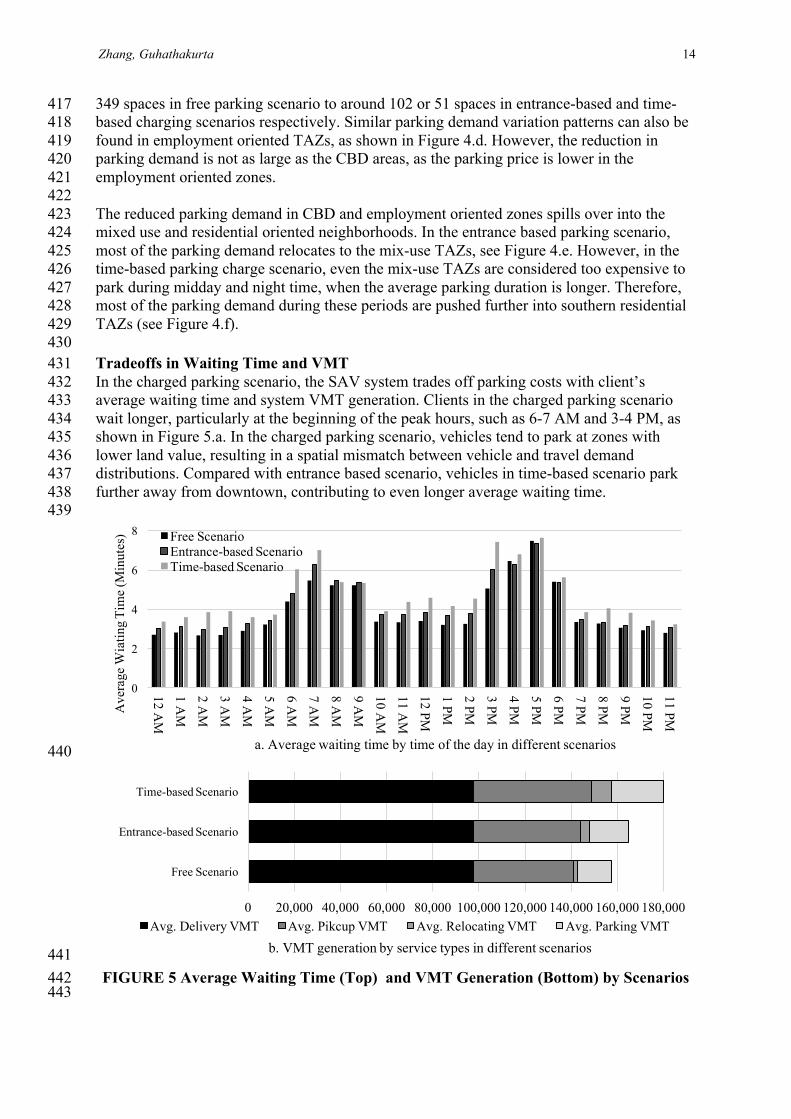
349 spaces in free parking scenario to around 102 or 51 spaces in entrance-based and time-417 based charging scenarios respectively. Similar parking demand variation patterns can also be 418 found in employment oriented TAZs, as shown in Figure 4.d. However, the reduction in 419 parking demand is not as large as the CBD areas, as the parking price is lower in the 420 employment oriented zones. 421 422 The reduced parking demand in CBD and employment oriented zones spills over into the 423 mixed use and residential oriented neighborhoods. In the entrance based parking scenario, 424 most of the parking demand relocates to the mix-use TAZs, see Figure 4.e. However, in the 425 time-based parking charge scenario, even the mix-use TAZs are considered too expensive to 426 park during midday and night time, when the average parking duration is longer. Therefore, 427 most of the parking demand during these periods are pushed further into southern residential 428 TAZs (see Figure 4.f). 429 430 Tradeoffs in Waiting Time and VMT 431 In the charged parking scenario, the SAV system trades off parking costs with client’s 432 average waiting time and system VMT generation. Clients in the charged parking scenario 433 wait longer, particularly at the beginning of the peak hours, such as 6-7 AM and 3-4 PM, as 434 shown in Figure 5.a. In the charged parking scenario, vehicles tend to park at zones with 435 lower land value, resulting in a spatial mismatch between vehicle and travel demand 436 distributions. Compared with entrance based scenario, vehicles in time-based scenario park 437 further away from downtown, contributing to even longer average waiting time. 438 439

440

441 FIGURE 5 Average Waiting Time (Top) and VMT Generation (Bottom) by Scenarios 442

443

0

2

4

6

8

12 AM

1 AM

2 AM

3 AM

4 AM

5 AM

6 AM

7 AM

8 AM

9 AM

10 AM

11 AM

12 PM

1 PM

2 PM

3 PM

4 PM

5 PM

6 PM

7 PM

8 PM

9 PM

10 PM

11 PMAve

rage

Wia

ting

Tim

e (M

inut

es)

a. Average waiting time by time of the day in different scenarios


0 20,000 40,000 60,000 80,000 100,000 120,000 140,000 160,000 180,000

Free Scenario

Entrance-based Scenario

Time-based Scenario

b. VMT generation by service types in different scenariosAvg. Delivery VMT Avg. Pikcup VMT Avg. Relocating VMT Avg. Parking VMT


The VMT generation is significantly higher in charged parking scenarios, see Figure 444 5.b. The SAV system generates 158,308 VMT per day in free parking scenario. The VMT 445 generation increases by 5% and 14%, respectively, in entrance-based and time-based 446 charging scenarios. In summary, the SAV system accounts for increases in parking costs by 447 increasing average waiting time and generating more VMT, both of which have negative 448 social externalities. Therefore, policy makers need to design policies that combine empty 449 VMT charges together with parking prices to reduce the negative environmental impacts, 450 such as energy consumption and pollutant emissions. 451 452

MODEL VERIFICATION AND VALIDATION 453 The trip generation process is validated by comparing the distributions of trip length and 454 departure time from the simulation results with Atlanta travel survey. The Chi-square 455 goodness of fit test results for trip length and departure time distributions are 0.96 and 0.98, 456 respectively, indicating that the simulated distributions are not significantly different from the 457 weighted Atlanta travel survey observations. 458

The vehicle movements are traced to verify the vehicle activities implementation 459 process. Figure 6 illustrates the travel path for a randomly selected vehicle in one simulation 460 day. The sequence of the visited nodes is labeled. The vehicle starts service at 5:31 AM and 461 ends service by 7:52 PM. 30 trips are fulfilled throughout the day. There are three ride-462 sharing trips, two of which involve intra-zonal travel and, therefore, are not reflected in 463 Figure 6. The vehicle spends approximately 7.2 hours serving clients, and 0.9 hours 464 relocating and navigating to parking lots. The vehicle checks into parking lot six times and is 465 parked for approximately 1.01 hours each time (excluding the last overnight parking). 466 467

468 FIGURE 6 Vehicle Travel Path Example 469


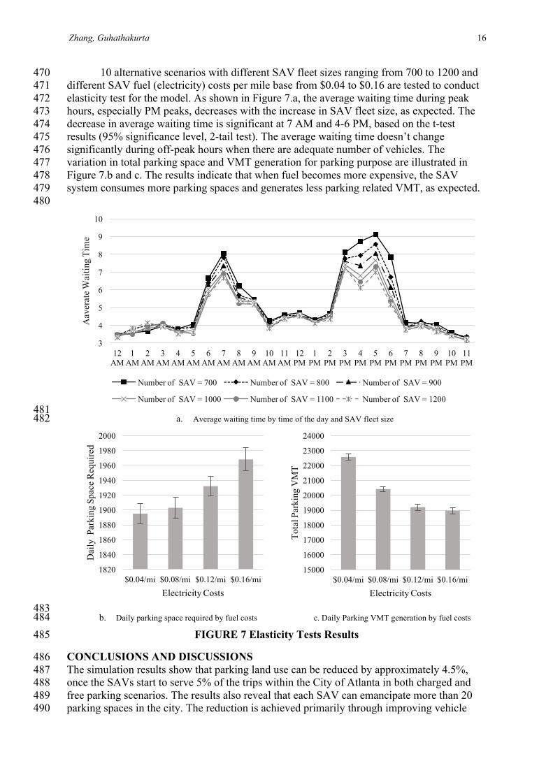
10 alternative scenarios with different SAV fleet sizes ranging from 700 to 1200 and 470 different SAV fuel (electricity) costs per mile base from $0.04 to $0.16 are tested to conduct 471 elasticity test for the model. As shown in Figure 7.a, the average waiting time during peak 472 hours, especially PM peaks, decreases with the increase in SAV fleet size, as expected. The 473 decrease in average waiting time is significant at 7 AM and 4-6 PM, based on the t-test 474 results (95% significance level, 2-tail test). The average waiting time doesn’t change 475 significantly during off-peak hours when there are adequate number of vehicles. The 476 variation in total parking space and VMT generation for parking purpose are illustrated in 477 Figure 7.b and c. The results indicate that when fuel becomes more expensive, the SAV 478 system consumes more parking spaces and generates less parking related VMT, as expected. 479 480

481 a. Average waiting time by time of the day and SAV fleet size 482

483 b. Daily parking space required by fuel costs c. Daily Parking VMT generation by fuel costs 484

FIGURE 7 Elasticity Tests Results 485

CONCLUSIONS AND DISCUSSIONS 486 The simulation results show that parking land use can be reduced by approximately 4.5%, 487 once the SAVs start to serve 5% of the trips within the City of Atlanta in both charged and 488 free parking scenarios. The results also reveal that each SAV can emancipate more than 20 489 parking spaces in the city. The reduction is achieved primarily through improving vehicle 490

3

4

5

6

7

8

9

10

12 AM

1 AM

2 AM

3 AM

4 AM

5 AM

6 AM

7 AM

8 AM

9 AM

10 AM

11 AM

12 PM

1 PM

2 PM

3 PM

4 PM

5 PM

6 PM

7 PM

8 PM

9 PM

10 PM

11 PM

Aav

erat

e Wai

ting

Tim

e

Number of SAV = 700 Number of SAV = 800 Number of SAV = 900

Number of SAV = 1000 Number of SAV = 1100 Number of SAV = 1200

1820

1840

1860

1880

1900

1920

1940

1960

1980

2000

$0.04/mi $0.08/mi $0.12/mi $0.16/mi

Dai

ly P

arki

ng S

pace

Req

uire

d

Electricity Costs

15000

16000

17000

18000

19000

20000

21000

22000

23000

24000

$0.04/mi $0.08/mi $0.12/mi $0.16/mi

Tota

l Par

king

VM

T

Electricity Costs


utilization intensity and reducing private automobile ownership. The results are consistent 491 with the parking demand model based on the hypothetical grid based setting [7] and the 492 Lisbon SAV simulation study [18]. 493

The simulation outcomes from charged and free parking scenarios suggest that 494 charged parking policies can effectively reduce the amount of parking in the CBD areas. 495 However, the demand for parking will be shifted to adjacent TAZs, resulting in larger VMT 496 generation more congestion and longer average waiting time. Furthermore, results from the 497 two charged parking scenarios suggest that when parking becomes more expensive; more 498 parking demand is pushed into low-income neighborhoods, which may lead to social 499 inequities. Therefore, policies to charge for parking need to be carefully considered to ensure 500 that such adverse effects are minimized. Examples of such policies may include 501 environmental impact fee for unoccupied VMT (i.e. relocation VMT and parking VMT) and 502 innovative congestion fee on SAVs to restrict excessive VMT generation. Furthermore, the 503 city may also propose smart parking policies, i.e. variable parking fee by time of day and by 504 location of parking lots to reduce parking land use by improving the occupancy rate of the 505 parking lots. 506

This study explores how the parking demand and parking land use may differ under 507 free and charged parking policies. There remain some limitations regarding the design of the 508 model, which deserves further explorations. To begin with, the parking destination choice is 509 made only based on total parking price, while other factors including travel demand and 510 vehicle distributions, are neglected. It will be ideal to design a parking lot searching 511 algorithm that combine vehicle relocation and parking step together to minimize the 512 operation costs of the system. Additionally, the model doesn’t offer an optimized solution for 513 urban parking land use design, which can be achieved by a centralized operation of SAV 514 system and will provide a more comprehensive picture for smart city development. More 515 studies should be devoted to examine how the SAV system can be integrated as part of the 516 sustainable urban growth by optimizing urban parking land use via smart parking pricing 517 policies. Finally, this model does not consider the environmental and social impacts of the 518 tradeoffs between VMT generation, congestion levels, and parking space reduction, which is 519 important for designing sustainable parking policies. Such tradeoffs can be examined with the 520 help of models that include a trip assignment function that dynamically updates congestion at 521 the road link level based on SAV travel patterns. 522 523

REFERENCES 524 525 1. CityMobil2 Project. (n.d.). CityMobil2 Project. Retrieved February 15, 2016, from 526

http://www.citymobil2.eu/en/About-CityMobil2/Overview/ 527 2. Markoff, J. (2014). Google’s next phase in driverless cars: No steering wheel or brake pedals. 528

New York Times. 529 3. Coyne, J. Here’s your first look at Uber’s test car. Retrieved February 15, 2016, from 530

http://www.bizjournals.com/pittsburgh/blog/techflash/2015/05/exclusive-heres-your-first-531 look-at-ubers-self.html 532

4. U.S. Department of Transportation. (2016). DOT actions revis existing guidance and clear 533 administrative hudles for new automotive technology. Retrieved April 17, 2016, from 534 http://www.nhtsa.gov/About+NHTSA/Press+Releases/dot-initiatives-accelerating-vehicle-535 safety-innovations-01142016 536

5. Burns, L. D., Jordan, W. C., & Scarborough, B. A. (2013). Transforming personal mobility. 537 Earth Island Institute, Columbia University. 538


6. Fagnant, D. J., & Kockelman, K. M. (2014). The travel and environmental implications of 539 shared autonomous vehicles, using agent-based model scenarios. Transportation Research 540 Part C: Emerging Technologies, 40, 1–13. 541

7. Zhang, W., Guhathakurta, S., Fang, J., & Zhang, G. (2015). Exploring the impact of shared 542 autonomous vehicles on urban parking demand: An agent-based simulation approach. 543 Sustainable Cities and Society, 19, 34–45. 544

8. Ford, H. J. (2012). Shared Autonomous Taxis: Implementing an Efficient Alternative to 545 Automobile Dependency. Princeton University. 546

9. Kornhauser, A. (2013). Uncongested mobility for all: New Jersey’s area-wide aTaxi system. 547 Princeton University. Operations Research and Financial Engineering. Retrieved September, 548 23, 2013. 549

10. Bridges, R. (2015). Driverless Car Revolution: Buy Mobility, Not Metal. Retrieved from 550 Amerzon.com 551

11. Albright, J., Bell, A., Schneider, J., & Nyce, C. (2016). Marketplace of change: Automobile 552 insurance in the era of autonomous vehicles. KPMG. 553

12. Barclays. (2016). Disruptive Mobility: A Scenario for 2040. Barclays Research. 554 13. Corwin, S., Vitale, J., Kelly, E., & Cathles, E. (2016). The Future of Mobility. Deloitte 555

University Press. 556 14. Fagnant, D. J., Kockelman, K. M., & Bansal, P. (2015). Operations of Shared Autonomous 557

Vehicle Fleet for Austin, Texas, Market. Transportation Research Record: Journal of the 558 Transportation Research Board, (2536), 98–106. 559

15. Zhang, W., Guhathakurta, S., Fang, J., & Zhang, G. (2015). The Performance and Benefits of 560 a Shared Autonomous Vehicles Based Dynamic Ridesharing System: An Agent-Based 561 Simulation Approach. In Transportation Research Board 94th Annual Meeting. 562

16. Greenblatt, J. B., & Saxena, S. (2015). Autonomous taxis could greatly reduce greenhouse-563 gas emissions of US light-duty vehicles. Nature Climate Change. 564

17. Chen, T. D., Kockelman, K. M., & Hanna, J. P. (2016). Operations of Shared Autonomous, 565 Electric Vehicle Fleet: Two Implications of Vehicle and Charging Infrastructure Decisions. 566

18. International Transport Forum. (2015). Urban Mobility System Upgrade: How shared self-567 driving cars could change city traffic. 568

19. Spieser, K., Treleaven, K., Zhang, R., Frazzoli, E., Morton, D., & Pavone, M. (2014). Toward 569 a systematic approach to the design and evaluation of automated mobility-on-demand 570 systems: A case study in Singapore. In Road Vehicle Automation (pp. 229–245). Springer. 571

20. Rigole, P.-J. (2014). Study of a Shared Autonomous Vehicles Based Mobility Solution in 572 Stockholm. 573

21. Shen, W., & Lopes, C. (2015). Managing Autonomous Mobility on Demand Systems for 574 Better Passenger Experience. In PRIMA 2015: Principles and Practice of Multi-Agent 575 Systems (pp. 20–35). Springer. 576

22. ARC. (2011). Household Travel Survey Final Report. Retrieved May 25, 2016, from 577 http://www.atlantaregional.com/transportation/modeling/household-travel-survey 578

23. CAP. (2014). Parking Today: Downtown Atlanta Parking Assessment Existing Conditions. 579 Retrieved from http://www.atlantadowntown.com/_files/docs/existing-conditions-580 download.pdf 581

582

parking spaces in the age of shared autonomous …docs.trb.org/prp/17-05399.pdf102 included parking...

Documents