PETTER LUNDBORG, ANTON NILSSON, DAN-OLOF ROOTH 2013:2

Parental Education and

Offspring Outcomes:

Evidence from the Swedish

Compulsory Schooling

Reform

i

Abstract

In this paper, we exploit the Swedish compulsory schooling reform in order to estimate

the causal effect of parental education on son's outcomes. We use data from the Swedish

enlistment register on the entire population of males and focus on outcomes such as

cognitive skills, non-cognitive skills, and various dimensions of health at the age of 18.

We find significant and positive effects of maternal education on sons' skills and health

status. Although the reform had equally strong effects on father’s education as on

mother’s education, we find little evidence that paternal education improves son’s

outcomes.

Contact information

Petter Lundborg, Lund University, Department of Economics

Anton Nilsson, Lund University, Department of Economics

Dan-Olof Rooth, Linneaus University, Linnaeus University Centre for Labour Market

and Discrimination Studies

0

1 Introduction An individual’s success in life is to an important extent determined by his or her abilities and

health capital, as formed in childhood and youth. In the literature on skill formation, cognitive

and non-cognitive skills during childhood and adolescence have been found to predict adult

outcomes, such as education, income, and engagement in criminal activities and risky

behaviors (Currie and Thomas 1999; Duckworth and Seligman 2005; Heckman et al. 2006;

Cunha and Heckman 2009; Lindqvist and Vestman 2011). Similarly, a recent literature,

spanning over medicine as well as economics, shows the importance of early life health for a

number of adult outcomes (see, for example, the recent surveys be Currie 2009 and Almond

and Currie 2011).

But what determines a person's abilities and health in childhood and adolescence? A key

factor is believed to be the human capital of one's parents. Children of more highly educated

parents tend to have better outcomes along a number of dimensions, such as health and

cognition, and, ultimately, labor market outcomes (see Currie 2009 for an overview). In

particular, maternal education is widely believed to be of great importance and numerous

studies across all types of countries have found a strong correlation between maternal

education and various child outcomes, such as health, mortality, and schooling (see for

instance Haveman and Wolfe 1995).

It is not clear, however, how one should interpret the correlation between maternal

education and children's outcomes. Is it that maternal education actually improves child

outcomes in a causal sense? In such a case, the returns to schooling would extend beyond the

individual himself to also include his offspring’s returns. Moreover, maternal education would

then be an important mechanism through which inequality is transmitted across generations.

Unfortunately, there is very little evidence on the causal effect of parental education on child

outcomes. There are a few studies in a developing context where a causal effect of mother's

education is implied but it is unclear to what extent these results generalize to developed

countries (Breiova and Duflo; Chou et al. 2007). For developed countries, the evidence to

date is also very limited and the few existing studies reach rather different conclusions about

the role of maternal education (Currie and Moretti 2003; McCrary and Royer 2011;

Lindeboom et al. 2009; Chevalier and Sullivan 2007; Carneiro et al. 2012).1 Clearly, the

limited evidence makes it difficult to conclude that the relationships between parental

education and child outcomes estimated in the literature are causal and we are left wondering

if the relationships mainly reflect the influence of hard-to-observe factors, such as genes,

environment , and family background.

In this paper, we contribute to the literature by providing new evidence on the causal

effect of mother's and father's schooling on their son's health and skills. We do so by

exploiting the Swedish compulsory schooling reform, which was rolled out over the country

during the 50s and 60s. An important feature of our identification strategy is that the timing of

1 We review these studies in more detail below.

1

the reform varied across municipalities, which gives as variation in reform exposure both

within and between cohorts. This provides us with plausibly exogenous variation in

schooling, which we exploit in order to estimate the causal effect of schooling on offspring

outcomes. The crucial assumption of our identification strategy is that conditional on birth

cohort fixed effects, municipality fixed effects, and municipality-specific linear trends,

exposure to the reform is as good as random. We provide a set of robustness checks, which

we argue show that this assumption is valid.

Our empirical strategy requires data on parental education and children's outcomes. For

this purpose, we use register-based data on the universe of individuals that were exposed to

the schooling reform, which includes information on education, place of residence, and date

of birth. By the use of personal identifiers, we have linked this data on the parental generation

to register-based data on their children, taken from the Swedish military enlistment register.

Since females are not obliged to enlist for the military in Sweden, this means that we are only

able to study outcomes among men. The benefit of the enlistment register, however, is that it

includes information on more or less the entire population of men, since enlisting for the

military was mandatory in Sweden during the time period considered. This gives us

considerable statistical power in our empirical analyses as well as an unusually high degree of

representativeness.

Another important feature of our data is that health and abilities are measured at age 18.

Many previous studies have focused on the effect of parental schooling on child outcomes

already at birth or at very early stages of life, although it is known that many personal

characteristics, such as cognitive and non-cognitive skills, are not yet fully developed at these

early ages (Cunha et al. 2006). We are aware of no previous study that considered the effect

of parental schooling on a wide range of offspring outcomes at age 18 and by doing so, our

study may thus be more suggestive of the more permanent consequences of parental education

on the outcomes of children.

Our results show that greater parental education improves outcomes in the next

generation along a number of dimensions, but that this effect is almost exclusively found for

mother's education. In particular, we find that maternal education improves cognitive and

non-cognitive skills, as well as overall health, and leads to greater stature. Interestingly, the

effects are of equal magnitude for both skills and health. We also provide some clues to

possible mechanisms behind these results; whereas greater maternal education leads to higher

income, higher quality spouses, reduced fertility, and an increased probability of continuing

schooling beyond elementary school, none of these effects are present among the fathers who

increase their schooling in response to the reform. Overall, our results provide new evidence

on the beneficial impact of maternal education across generations and shed light on one

possible mechanism through which inequality is transmitted across generations.

The paper is organized as follows. In Section II we discuss the literature on the topic

and the potential mechanisms through which education could affect child health. In Section

III, we outline of empirical strategy and provide details on the Swedish schooling reform.

2

Section IV discusses the data we use and in Section V we present the results. Section VI

concludes.

2 Background Why should parental education matter for child outcomes? Commonly discussed causal

pathways have been the improved knowledge and the greater economic resources that follow

with greater education. The latter pathway refers to the fact that higher education usually also

means higher income. To the extent that this also spills over to the child, this would be one

mechanism through which parental education affects child outcomes. Causal evidence for

such income effects were obtained in Dahl and Lochner (2012), where increases in maternal

income resulting from changes in the earned income tax credit showed a positive effect on

children's math and reading test scores. The gains were largest for children from

disadvantaged families.2 Similar findings were reported in Duncan et al. (2011) and Milligan

and Stabile (2011), using quasi-experimental variation in government income transfers, and in

Løken et al. (2011), exploiting regional variation in the income boom that followed the

discovery of oil in Norway.

Possible explanations for the positive income effects include greater affordability of

health care inputs (Currie 2009). This mechanism should perhaps not be overemphasized in a

country like Sweden, however, where health care coverage is universal and of low cost. Still,

income may be related to the quality of neighborhoods and schools, as well as to the

affordability of cognitively stimulating material and activities (e.g., Yeung et al. 2002), which

may all generate links between parental income and child outcomes.

An alternative mechanism is that higher income is related to lower fertility, since time-

intensive child caring becomes more costly as income rises. To the extent that there is a trade-

off between child quality and child quantity (Becker and Tomes 1976), this suggests an

alternative explanation for the effect of education on child outcomes.3 In our empirical

analysis, we will consider to what extent income and fertility effects could explain the link

between parental education and child outcomes.

Besides increasing economic resources, it has been argued that education improves

productive efficiency in health production (Grossman 1972). This line of reasoning could

easily be generalized to investments in cognitive and non-cognitive skills and to investments

over generations, where, for instance, more well-educated parents would be more

knowledgeable in how to use various health inputs and time inputs in the production of child

2 Increased maternal income may also increase the bargaining power of women, which shifts household spending

towards items that women value more. Since mothers are often found to value the family's health more than

fathers do, this is as additional route through which income may affect children's health and skills (see Behrman

1997 for a survey).

3 An offsetting effect would be if parents with a high value of time invest less time in child health and the

production of skills. In countries like Sweden, however, there may be high-quality and low-cost substitutes such

as child care, with highly trained personnel.

3

quality. Such an increase in “productive efficiency” implies that additional education allows

an individual to obtain greater child outcomes from a given set of inputs. Similar to

productive efficiency, it is also possible that education facilitates allocative efficiency in

health production, meaning that more educated parents are better able to choose a better mix

of health inputs in the production of child health and skills (e.g., Thomas 1994).

It should be noted that any effects of parental education that are generated through

improved knowledge or increased resources would be magnified under positive assortative

mating. Improved education would then also lead to higher-quality spouses, which boosts

total resources and knowledge in the household. Since we have data on the spouse's

characteristics, we are able to shed light on this issue in our empirical analysis.

While our discussion so far has focused on a possible causal relationship between

education and child outcomes, any positive empirical relationship could also be generated

through non-causal mechanisms. In particular, since parents and children share common

genes, any relationship between them may be generated through unobserved genetic

endowments. More generally, preferences and personality traits, whether genetically induced

or not, may be shared by parents and children, which, again, may cause a positive relationship

between parental education and children's outcomes. A related hypothesis was formulated by

Fuchs (1982), who suggested that education and health were related through an individual's

time preferences. The argument is that both investments in health and education are of long-

run character, since the benefits in both cases occur in the future, and that future-oriented

individuals will thus invest in both. Translated to the parent-child relationship, it would mean

that future-oriented parents invest both in their children's health and skills and in their own

education but there may exist no causal relationship between the two types of outcomes. If

this or other underlying factors are the reason why parental education and child outcomes are

correlated, it would mean that policies that increase parental education would have no effect

on child outcomes.

What does then the existing literature say about the existence of a causal effect of

parental education on child outcomes? Unfortunately, there are rather few studies on the topic

and the existing ones reach quite different conclusions. Regarding health outcomes, Currie

and Moretti (2003) found that maternal education improved birth weight (and reduced

smoking) in the US, whereas McCrary and Royer (2011) found no effect on birth weight and

other birth outcomes using US data. As noted by Royer and McCrary, this most likely reflects

that different identification strategies were used. Currie and Moretti (2003) exploited variation

in the access to colleges, whereas McCrary and Royer used birth date variation to get

exogenous variation in schooling. The subgroups affected by the instruments therefore likely

differed between the studies.

Yet another source of exogenous variation in schooling was used in two studies in a UK

context. Lindeboom et al. (2009) used the compulsory schooling reform in 1947 in Britain to

estimate the causal effect of schooling on child health. They found no evidence of a causal

effect of parental schooling on child health outcomes at birth or at ages 7, 11, and 16.

However, due to a small sample size, their estimates suffered from a relatively low precision.

4

Exploiting the same reform, Chevalier and Sullivan (2007), obtained evidence of

heterogeneous effects and found that the most impacted groups experienced larger changes in

infant birth weight. One disadvantage of the British schooling reform was that it affected

entire cohorts, which makes it difficult to separate out reform effects from cohort effects.

In the spirit of Currie and Moretti (2003), Carneiro et al. (2012) used U.S data and

instrumented mother's education with variation in schooling costs during the mother's

adolescence. They found a significant effect of maternal education on child test scores, but

also on measures of behavior problems.

Other studies have tried to get at the causal effect of parental education on child

outcomes with alternative research designs. Lundborg et al. (2011) used both a twin design

and an adoption design and applied these to data from the Swedish enlistment register. Under

both designs, parental education was significantly related to improved cognitive skills, non-

cognitive skills, and health. A twin design was also adopted by Bingley et al. (2009), who

related parental education to children's birth weight, finding a small but significant effect.4

The different results in the literature should come as no surprise, since different outcomes are

studied, different identification strategies are used, and since the contexts are different. But as

noted by Currie (2009), the contrasting results also makes it difficult to clearly state that the

relationship between parental background and children's health is a causal relationship. In this

paper, we expect the instrument to mostly impact low-educated persons, who would not have

gone through an additional year of schooling, had they not needed to. For policy purposes,

this is a group of special interest, since compulsory schooling reforms may have a big impact

on exactly this group. Moreover, to date, there is no evidence that increasing the education of

these women would affect child outcomes, which is somewhat surprising, since one may

argue that the returns to increased schooling would in general be greater for this group.

3 Method

A. The Schooling Reform

The Swedish compulsory schooling reform has been previously described by Holmlund

(2008), Meghir and Palme (2005), and, more extensively, by Marklund (1980, 1981). Here,

we provide a brief overview of the reform. In the 1940s, prior to the implementation of the

reform, children in Sweden went to a common school (“folkskolan”) up until either 4th or 6th

grade. Individuals with sufficient grades were then selected for the junior secondary school

(“realskolan”), where they stayed for three, four or five years; the exact arrangements differed

from municipality to municipality. Individuals that were not selected for junior secondary

school had to remain in the common school until compulsory schooling was completed.

4 The estimates in the twin studies are identified for the (parental) twin pairs that differ in schooling. If such

differences are found all over the education distribution, twin estimates may come closer to estimating an

average treatment effect. However, this requires twins not to differ in other respects that are related to their

education as well as offspring outcomes.

5

Compulsory schooling spanned seven years, or in some municipalities (mainly in the large

cities) eight years.5

There was a growing political pressure for a schooling reform during the entire 1940s,

however. In particular, the Swedish educational system was deemed insufficient in light of the

many other Western countries that had already introduced eight or nine years of compulsory

schooling, or were about to do so. In 1948, a parliamentary committee delivered their

proposal to introduce a new compulsory school, consisting of nine compulsory years. In the

new compulsory school, students would be kept together up until 8th grade and in 9th grade

follow different tracks; this streaming in 9th grade was later abandoned, however.6 The

reform also affected the curriculum somewhat, mainly by introducing English as a

compulsory subject.

Rather than being introduced in the entire country at the same time, the schooling

reform was set to be implemented gradually, with the aim to enable evaluations of the

appropriateness of the reform before deciding whether to implement it nationwide.7

Beginning in 1949, 14 municipalities introduced the school reform. More municipalities were

then added year by year; the reform was generally implemented by all school districts within

the municipality, with the exception of the three big city municipalities of Stockholm,

Göteborg, and Malmö, where the reform was implemented in different parts of the

municipalities at different times. In 1962, the Swedish parliament decided that the reform

should be implemented throughout the country and that all municipalities needed to have the

new system in place no later than in 1969.

This paper is not the first to exploit the Swedish compulsory schooling reform as a

source of exogenous variation in schooling. Meghir and Palme (2005) established that the

reform increased educational attainment and led to higher labor incomes. They were also able

to account for selective mobility, that is, whether their results would be biased by individuals

moving to or from reform municipalities to choose suitable schooling for their children. They

found no evidence of this being the case. A study by Holmlund et al. (2011) used the reform

as an instrument for parental schooling, and found evidence of a causal effect of parent's

educational attainment on child's educational attainment.

Regarding health outcomes, Spasojevic (2010) used Swedish survey data and found

some weak evidence that one year of additional schooling generated by the reform led to a

better self-reported health and a higher likelihood of having a BMI (body mass index) in the

5 As children in Sweden in general start school during the calendar year they turn seven, this means that

compulsory schooling normally lasted until the age of 13 or 14. 6 The reform may thus also have affected class composition, due to the changes in the timing in ability tracking.

In particular, some students may benefit from having more high-ability individuals in their class after the reform

(e.g., Ding and Lehrer 2006). Moreover, patterns of assortative mating may be affected. We discuss these issues

in more detail in the Methods subsection. The streaming in 9th grade was abandoned in 1969. 7 During the assessment period, only municipalities that had shown interest in the reform were selected to

implement it, meaning that reform implementation was not random. Meghir and Palme (2003) as well as

Holmlund (2008) document that there is no evidence that reform implementation would be associated with

various personal characteristics however, although Holmlund points at the importance of controlling for

municipality fixed effects, birth year fixed effects, and municipality trends when using the reform as an

instrument for schooling. We return to these issues in the Econometric Method subsection.

6

healthy range. Meghir et al. (2012) considered hospitalizations and mortality among

individuals exposed to the reform, but found little evidence that more schooling would

improve individuals’ health in these respects. No previous study has examined the effects on

health and skills among children of those who were exposed to the reform.

B. Econometric Method

Our empirical model is based on the following two equations.

(1) Hc = α0 + α1S

p + α2Y

p + α3M

p + α4Trend

p + ε,

(2) Sp = β0 + β1R

p + β2Y

p + β3M

p + β4Trend

p + υ.

In these equations, c denotes the child and p one of his parents. S refers to parental years of

schooling, M is a set of municipality fixed effects, Y is a set of birth year fixed effects, Trend

is a set of municipality-specific linear trends, and H is the outcome of interest. R is a dummy

variable indicating whether the individual was exposed to the reform or not.

In order to obtain some “baseline results” regarding the relationship between parental

education and the various child outcomes, we first estimate OLS regressions based on

equation (1). Given that schooling is likely to be correlated with various omitted factors such

as abilities and other personality traits, these results cannot be interpreted as causal effects of

parental schooling. We therefore apply Two Stage Least Squares (2SLS), using equation (2)

as the first stage, where schooling is instrumented by reform status. The identification of α1,

the coefficient of interest, then relies upon the part of variation in parental schooling that is

generated by the reform. Our empirical strategy is similar to the one used in previous reform-

based papers, such as Black et al. (2005). The first-stage is based on a difference-in-

differences approach (DiD), where individuals treated by the reform are compared to

individuals in the same municipality before treatment as well as to individuals in other

municipalities, while taking possible trends at the municipality level into account.

2SLS estimates can be interpreted as weighted averages of the causal responses of those

individuals whose treatment status is changed by the reform instrument, given that certain

conditions are fulfilled (e.g., Angrist and Imbens 1995; Imbens and Angrist 1994). First of all,

the independence assumption requires that reform exposure is as good as random, conditional

upon the controls included. As we expect reform implementation to be correlated with both

municipality and time specific effects, these need to be controlled for. Reform implementation

may, however, also be correlated with factors that change both within municipalities and over

time. In our main specification, we account for this by including municipality-specific trends.

As an alternative way to pick up such characteristics that may change both over time and in

space, we explore specifications using interactions between home county and birth year.

In order for the independence assumption to hold, it is also important that individuals do not

choose their reform status. This could be the case if individuals moved to or from reform

municipalities in some systematic way. We are not able to investigate this issue in detail, but

7

rely on Meghir and Palme (2005), who had access to data on municipality of birth as well as

municipality at school age, and, as mentioned, obtained no evidence of selective mobility

being an issue.8

A second assumption required for 2SLS to reflect an average of causal responses is the

exclusion restriction, saying that the reform should only affect child outcomes through its

effect on years of parental schooling. This assumption could be violated if the reform also

affected the quality of the education provided. In particular, it is probable that some schools

hired a number of teachers in advance and started re-organizing already some time before the

introduction of the reform, and that for some schools there was a shortage of teachers and a

lower organizational quality right after the reform was implemented. In order to avoid such

short-run adjustment effects, we will not consider individuals born in the first reform cohort

and in the cohorts immediately following and preceding it.9

Moreover and as already mentioned, class composition was influenced by the reform

since ability tracking was postponed. This can affect peer group composition as well as

patterns of assortative mating. Additionally, a more highly educated population in general

may have indirect effects on individuals’ outcomes through better (or worse) labor market

opportunities. It is unclear to what extent such general equilibrium effects would be present

and we note that most studies exploiting schooling reforms would be subject to this risk.

As a third condition, the reform must, on average, affect educational attainment in order for it

to be used as a source of exogenous variation in schooling. It is also important that the effect

on educational attainment is rather strong. In the Results section, we show that this is indeed

the case, both among mothers and fathers.

Fourth and finally, the monotonicity assumption requires that the sign of the response to

the reform is homogenous in the study population. In our case, that is to say that no

individuals reduced their investments in schooling as a result of the reform. In principle, one

could imagine that some individuals who would have continued to higher education when not

affected by the reform instead choose to stop at nine years of schooling when forced to do at

least nine – for example due to changing preferences or institutional arrangements. While

such possibilities cannot be ruled out, we document that the reform rather had a positive

impact on the share of individuals obtaining more than nine years of education in our samples

of mothers as well as fathers.

8 They used two different approaches to investigate this. First, they re-estimated their regressions only including

individuals who did not change reform status as a result of moving to another municipality between birth and

school age. Second, they instrumented reform status using as instruments the reform status in the municipality of

birth (when this was available) as well as an indicator for whether the reform status in the municipality of birth

was known. 9 In line with adjustment effects, but also with the possibility that some individuals may not have been in the

right cohort according to their age or that the reform coding may be subject to some measurement errors,

Holmlund et al. (2008) documented that the Swedish compulsory schooling reform had a substantial impact on

educational attainment even in the cohort one year prior to the first reform cohort, as well as evidence of the

reform having a different effect on schooling in the first reform cohort and in the cohort right after it compared to

later cohorts. We tried to replicate this finding and obtained similar results, which is not surprising as the

datasets are similar.

8

4 Data Our dataset is constructed by integrating registers from Statistics Sweden (SCB) and the

Swedish National Service Administration. The former includes the Census of the population

and housing (“Folk- och bostadsräkningen”) from 1960, virtually covering the entire Swedish

population alive in this year, and the Multi-generation register (“Flergenerationsregistret”),

allowing us to link parent individuals to children born during later years. There is also data on

educational attainment as of 1999, which is expressed in terms of the highest degree attained.

Based on this, a standard number of years of schooling has been assigned. Our data include

parents with information on educational attainment that are born between 1940 and 1957;

these are essentially the birth cohorts for which there is variation in whether the reform has

been implemented or not.

Data on home municipality is obtained from the Census of the population and housing;

there are 1,029 municipalities in our data. During the study period of time, Sweden was

divided into 25 counties. We obtain data on home county based on our data on home

municipality in 1960.

The reform assignment is based on an algorithm provided by Helena Holmlund, which

was described in Holmlund (2008).10

The algorithm uses historical evidence on reform

implementation and assigns the reform exposure variable to individuals depending on his or

her year of birth and home municipality in 1960. Individuals need to be in the correct grade

according to their age in order for the algorithm to correctly classify them with respect to

reform status.

As noted earlier, the reform was implemented for all school districts at the same time in

entire municipalities, with the exception of the three big city municipalities in Sweden, where

implementation was more gradual. Applying the algorithm provided by Holmlund, the

implementation cohort in these three cities is only set to one when the entire municipality has

transferred to the new system; parishes within these municipalities that are known to have

implemented the reform in the first years are dropped. Still, it is possible that measurement

errors are larger in these three city municipalities compared to the rest of the country

(Holmlund 2008). In one of our sensitivity checks, we therefore drop these cities.

Data on offspring health and skills are obtained from the military enlistment records,

covering individuals born between 1950 and 1979, although no individuals from the earlier

cohorts will be used as parents must have been born no earlier than in 1940.11

At the time

under study, the military enlistment was mandatory for men in Sweden, with exemptions only

granted for institutionalized individuals, prisoners, individuals that had been convicted for

heavy crimes (which mostly concerns violence-related and abuse-related crimes) and

individuals living abroad. Individuals usually underwent the military enlistment procedure at

10

We are grateful to Helena for generously sharing the reform coding with us.

11 Also, the children had to live in Sweden during 1999 since the enlistment information was initially collected

for the 1999 population data.

9

the age of 18 or 19.12

Refusal to enlist lead to a fine, and eventually to imprisonment,

implying that the attrition in our data is very low; only about 3 percent of each cohort of

males didn’t enlist.

A. Outcome Variables

Our analysis uses several different measures of individuals’ overall health status which are

available in the military enlistment data. First, based on the conscript's health conditions and

the severeness of these, the National Service Administration has assigned each conscript a

letter between A to M (except “I”), or “U,” ”Y,” or “Z”. The assignment is based on both

physical and mental conditions, and we will refer to this measure as “global health”. The

closer to the start of the alphabet the letter assigned to the individual is, the better his general

health status is considered to be. ”A” thus represents more or less perfect health, which is

necessary for ”high mobility positions” (for example light infantry or pilot) and has been

assigned to about two-thirds of all individuals for which there is non-missing data. For combat

positions, individuals must have been assigned at least a “D”; individuals with a “G” or lower

are only allowed to function in “shielded positions” such as meteorology or shoe repairing.

Individuals assigned a “Y” or “Z” (in total 6 percent of all individuals in our full sample) are

not allowed to undergo education within the military. ”U” indicates that global health status

has not been decided, and we treat this as missing. As our first measure of overall health, we

transform ”A” into 0, ”B” into -1, “C” into -2 etc., ”Y” into -12 and ”Z” into -13, and then

normalize this variable to have standard deviation one. For the ease of interpretation and

comparison, all the non-binary outcome variables used in our analysis will also be normalized

to have standard deviation one.

The determination of individuals’ health that underlies the assignment of the global

health variable is based on a health declaration form that the individual has filled in at home

and has to bring with him, combined with a general assessment of the individual’s health

lasting for about 20 minutes, performed by a physician. Before meeting the physician, the

individual has undergone a number of physical capacity tests and has met with a psychologist

who, if necessary, can provide the physician with notes regarding the individual’s mental

status. The individual is expected to bring any doctor’s certificate, health record, drug

prescription or similar proving that he actually suffers from the conditions he has reported in

his health declaration, making “cheating” difficult. Moreover, the incentives to cheat may be

low since almost everyone was required to undergo military service during the study period of

time. It is an important advantage of our data that health status is not simply self-reported, but

also based on obligatory assessments. Consequently, measurement errors for example

originating from differences in health-seeking behaviors or in health awareness, which may be

present in sources like hospital and insurance records or standard self-evaluations, should be

less of an issue.

12

According to our data, 80 percent of all individuals enlisted during the year they turned 18, whereas 18 percent

did so during the year they turned 19. Virtually no individuals enlisted before the age of 18.

10

As an alternative measure of overall health, we use height, as determined at military

enlistment. An adult’s height relates to many aspects of their childhood health status (see, e.g.,

Bozzoli et al. 2009) and has been referred to as “probably the best single indicator of his or

her dietary and infectious disease history during childhood” (Elo and Preston 1992). It has

been documented that children of parents with more years of education tend to be taller (e.g.,

Thomas 1994), although it is not clear if this relationship reflects a causal effect.

In addition to height, we make use of three different “physical test variables” from the

military enlistment records, which relate to certain dimensions of individuals’ health and

capacities. First of all, we make use of physical work capacity, measured as the maximum

number of watts attained when riding on a stationary bike (for about five minutes). Measures

of this type are often referred to as Maximum Working Capacity and have consistently been

associated with lowered risk of premature deaths from mainly cardiovascular diseases and to a

lesser extent with lowered risk of cancer-related mortality (Ekelund et al. 1988; Slattery and

Jacobs 1988; Blair et al. 1989; Sandvik et al. 1993).13

The measure is closely related to

maximum oxygen uptake (VO2 max), which has been labeled as “the single best measure of

cardiovascular fitness and maximal aerobic power” (Hyde and Gengenbach 2007). A large

number of studies have found a positive relationship between parents’ schooling and child or

adolescent physical activity (Stalsberg and Pedersen 2010), which, if causal, would also

suggest that more parental education may lead to a higher physical capacity of their children.

Second and third, we include indicators of obesity and hypertension. Using standard

definitions, we classify individuals as obese if their BMI (kg/m2) is higher than or equal to 30

and as hypertensive if either their systolic blood pressure is higher than or equal to 140 mmHg

or their diastolic blood pressure is higher than or equal to 90 mmHg. Both obesity and

hypertension are well-known risk factors of diseases such as cardiovascular diseases and

diabetes (e.g., Poirier et al. 2006; Sowers et al. 2001). Obesity can also lead to discrimination

in the labor market (e.g., Lundborg et al. 2010). It has been documented that children of

parents with more years of education tend to have lower incidences of obesity and higher

incidences of hypertension (e.g., Lamerz et al. 2005; Coto et al. 1987).

We also include measures of cognitive and noncognitive ability. Cognitive ability is

measured through written tests of logical, verbal, spatial and technical skills. Based on his

results on these tests, the individual has been assigned a number on a nine-point scale,

approximating a normal distribution.

Noncognitive ability is also measured on a scale between 1 and 9 which approximates a

normal distribution. The assignment of this number is done by a psychologist, based on a

semi-structured interview lasting for about 25 minutes, whose objective is “to assess the

conscript’s ability to cope with the psychological requirements of the military service and, in

extreme case, war” (Lindqvist and Vestman 2011). This in particular implies an assessment of

13

Moreover, in a field experiment, Rooth (2011) found that physical capacity (as measured at the Swedish

military enlistment) has positive effects on subsequent labor market outcomes in terms of a higher probability to

receive a callback for a job interview. Individuals with higher physical capacity were also found to have higher

earnings.

11

personal characteristics such as willingness to assume responsibility, independence, outgoing

character, persistence, emotional stability and power of initiative. In addition, an important

objective of the interview is to identify individuals who are considered particularly unsuited

for military service, which includes individuals with antisocial personality disorders,

individuals with difficulty accepting authority, individuals with difficulties adjusting to new

environments and individuals with violent and aggressive behavior (Andersson and Carlstedt

2003; Lindqvist and Vestman 2011).

B. Sample Construction

Our estimation sample is constructed by imposing the following restrictions. For the child

generation, we exclude the small number of women (0.25 percent) volunteering for the

military. Next, for the parent generation, we exclude all individuals for which no male child is

observed in our data (39 percent). Parents with missing data on home municipality are then

excluded (1 percent), and of the remaining parents, individuals in municipalities for which the

algorithm has not been able to assign reform status are also excluded (11 percent). Moreover,

in order to avoid short-run adjustment effects of the reform as well as misclassification of

individuals right around the implementations, we exclude individuals belonging to the first

reform cohort, and the cohorts immediately preceding and following it (14 percent). Finally,

considering only children for which at least one parent is observed in the sample, our

estimation sample includes 503,768 individuals in the child generation. For 405,845 of these,

their mother is observed in the estimation sample, and for 326,600 their father is observed.

The reason why the number of children for which a father is observed is smaller than the

number of children for which a mother is observed is that fathers are generally older and are

thus more likely to have been born before the start of our sample period.

In Table 1A, we provide descriptive statistics for the estimation sample.14

Regarding the

child generation, the average birth year is 1971. Both hypertension and respiratory conditions

are quite common health problems in this population as they affect 19 and 17 percent of the

individuals, respectively. Suffering from obesity or being diagnosed with a mental condition

is much less common; these affect only 2 and 4 percent of the individuals, respectively.

5 Results

A. OLS Relationships

In Table 2, we present OLS results on the relationship between parental education and son's

outcomes, based on equation (1). All estimates of parental schooling are statistically

significant and are in general similar between mother’s and father’s years of schooling. The

strongest effects are found for cognitive and non-cognitive ability, where one year of maternal

education is associated with about 0.12 standard deviations higher cognitive ability and 0.07

14

Table 1B shows descriptive statistics for the subsamples being exposed or not exposed to the reform.

12

standard deviations higher non-cognitive ability. For fathers, one additional year of schooling

is associated with 0.11 standard deviations higher cognitive ability and 0.06 standard

deviations higher non-cognitive ability.

While the coefficients for our health and physical test variables are smaller in

magnitude compared to the ones obtained for cognitive and non-cognitive abilities, our results

in most cases suggest better outcomes for sons with higher educated parents. In particular, one

additional year of parental education implies between 0.01 and 0.02 standard deviations better

global health, about 0.03 standard deviations taller height, and about 0.05 standard deviations

better physical capacity. Individuals with more highly educated parents are also significantly

less likely to suffer from obesity, where one year of parental schooling is associated with 0.24

percentage points lower probability of being obese. Contrastingly, and perhaps more

unexpectedly, our data suggest a positive relationship between parental schooling and the

incidence of hypertension.

B. First Stage Results

Next, we turn to our instrumental variables estimates. In order for the reform instrument to be

valid, it must have a strong effect on parental years of schooling. We first investigate this by

considering the regression results for equation (2), which are presented in Table 3. In

specification (A), we only include birth cohort fixed effects, whereas specification (B) also

controls for municipality fixed effects. In addition to these controls, specification (C) adds

controls for county-by-year effects, whereas specification (D) instead adds controls for

municipality-specific linear trends.

The simplest specification in column A shows a very strong relationship between the

reform and average years of schooling, with coefficients around 0.6 and F-values of about

2000 and 5000 for women and men, respectively. Both the coefficients and the F-statistics

drop heavily when taking municipality factors into account, however, as shown in column B,

where coefficients are around 0.2 and F-values about 10. These are less convincing results as

the rule of thumb (e.g., Staiger and Stock 1997) suggests that F-values should be at least 10

(and preferably higher) for the IV method to be valid.

In (C), we then add interactions between home county and year of birth. This

specification is more flexible in that it allows for any kind of time-varying behavior in

schooling enrollment decisions, given that these behaviors are the same within each county.

This may be reasonable, for example, if preferences, demographics or labor market conditions

are similar within counties. F-statistics now increase to 30 and 40 and the coefficients on

reform status have increased somewhat in magnitude.

It is still possible that some unobserved factors vary also between municipalities within

a county as well as over time. In specification (D), we therefore instead include municipality-

specific linear trends. This implies a very large set of controls as there are more than one

thousand municipalities in our data. The coefficients obtained are very similar to those in

column C, and the results suggest that the reform on average increased mother’s educational

attainment by 0.25 years and father’s educational attainment by 0.35 years. Both F-statistics

13

are about 45, showing a strong effect of the reform. It is important to note that the reform

predicts mother’s and father’s education almost equally strongly, because this means that, for

a given relationship between parental schooling and child’s outcomes, significant effects on

child’s outcomes are equally likely to show up for both parents’ education.15

C. Results

Having established that our first-stage is strong, we next turn to our 2SLS estimates, shown in

Table 4. We again consider four sets of models, corresponding to those for which the first

stage was investigated above. First, in panel A, we report results from regressions where we

only control for birth year fixed effects, whereas in the models in panel B we then also control

for municipality fixed effects. As can be seen, there are a large number of significant effects,

particularly in panel A. For example, our estimates in both panel A and B suggest that

parental education leads to a higher physical capacity and a higher cognitive ability, both for

maternal and paternal education. Some coefficients have unexpected signs; for example, the

results in panel A suggest negative effects on global health. Moreover, all the coefficient

estimates in these panels suggest positive effects on the incidence of hypertension.

We then turn to our results in the models including larger sets of controls, which we

expect to produce more reliable results, given that reform implementation may be correlated

with factors that change over time within geographical regions or municipalities, and given

that these models have stronger first stages than those in panel B. Beginning with the results

in panel C, where county-by-year effects have been included, mother’s education is found to

significantly influence three out of our seven outcome variables. First of all, the results

suggest that mother’s education has strong beneficial effects on the child’s general health

status, as measured by global health and height. In terms of standard deviations, the effect of

maternal schooling on global health is just somewhat higher than the effect on cognitive

ability, whereas the effect on height is somewhat lower; both these estimates are much higher

than the corresponding estimates in the OLS case and somewhat stronger than those obtained

in panel B. The effects on more specific health outcomes, that is, physical capacity, obesity,

and hypertension are now all insignificant and smaller in magnitudes. Cognitive ability is

positively affected by mother’s schooling, with an estimate that is almost identical to its OLS

counterpart, but also to the result in panel B; one year of maternal schooling is associated with

an 0.11 standard deviations higher cognitive ability. There is no evidence that mother’s

schooling would significantly influence non-cognitive ability.

Our results for mothers schooling in panel D, our preferred specification where instead

municipality-specific trends have been included, are very similar to those in panel C. This is

reassuring as quite different methods to deal with time- and municipality-varying factors have

been used. The effect on cognitive ability is even identical up until four decimal places in

15

Our first stage results are similar to those obtained by other studies using the Swedish compulsory schooling

reform. For example, Holmlund (2008) finds coefficients of 0.20 and 0.28, and Holmlund et al. (2008) find

coefficients of 0.26 and 0.33, for women and men respectively. Moreover, Meghir and Palme (2005) find

coefficients of 0.34 and 0.25. Their study is somewhat different, however, in that only two birth cohorts (1948

and 1953) were used, and consequently municipality-specific trends have not been included.

14

panel D compared as compared to column C, whereas the effect on global height is somewhat

lower in panel D and the one on height just somewhat higher. The effect on noncognitive

ability has now become significant at the 10 percent level in panel D, suggesting that mother’s

schooling may play a role in shaping individual characteristics such as willingness to assume

responsibility, independence and outgoing character. All the significant effects are in fact very

similar in magnitudes and amount to about 0.1 standard deviations. Again, effects on more

specific health outcomes are all insignificant as well as small.

Compared to mother’s education, there is much less evidence that father’s education

influences the outcomes of the child in panel C as well as in panel D. In particular, the

coefficients on global health, height, cognitive ability and noncognitive ability are all

substantially closer to zero compared to the results for mother’s schooling, and statistically

insignificant. Not only point estimates, but also the standard errors are in general smaller on

the coefficients for father’s education compared to mother’s, showing that our insignificant

results for father’s education are not simply due to lack of power. Could it be simply that

different LATEs are estimated in the group of mothers and fathers and that the estimates

therefore are not strictly comparable? Most likely not, since the average number of years of

schooling were evenly distributed among mothers and fathers, instead suggesting that the

LATEs estimated for mothers and fathers are in fact rather similar. In one case, do our results

suggest that father’s schooling is associated with better outcomes; in terms of physical

capacity. This result is consistent with a paternal influence on physical activity. Just like our

results for maternal schooling, the effect of one year of paternal schooling on this outcome is

about 0.1 standard deviations.16

While having in mind that our results may only be viewed as capturing causal effects on

offspring individuals with low educated parents, it should be noted that our results for global

health, in the models with larger sets of controls, are much in line with those reported in

Lundborg et al. (2011), where father's education was insignificant whereas mother's education

had a significant coefficient of 0.05 and 0.17 when applying the adoption and twin design,

respectively. Our estimate for mother’s education thus falls right in between these estimates.

Contrastingly, however, our results for cognitive skills suggest a much stronger influence of

mother's schooling compared to the ones reported by Lundborg et al. (2011) as our

coefficients are more than twice as large. This may reflect the fact that our instrument affected

parents with low levels of education. Moreover, our findings that cognitive abilities,

noncognitive abilities, and height are not significantly related to father's schooling stand in

stark contrast to the results in Lundborg et al. who even find that father's education is more

important than mother's education.

Although the outcomes studied are somewhat different, we can also compare our results

with those of Carneiro et al. (2012), who found that one additional year of maternal schooling

increases (white) children’s performance at a math test at age 7-8 by about 0.10 standard

16

Instead of using municipality-specific trends, one may also include year-of-implementation-specific trends to

deal with the possibility of differential trends in treatment and control municipalities. Doing this yields almost

identical results.

15

deviations and decreases their “behavioral problems index” (BPI) by 0.09 standard deviations.

The results when only including girls were even stronger, whereas no statistically significant

effects for these outcomes were found when only including boys. While this may be due to

the relatively small sample size, the coefficients were, in general, also smaller in magnitudes

for boys than for girls. Note, however, that the group affect by the instrument in their study

most likely differ from the group affected by our instrument, which may explain the

difference in findings.

Our results stand somewhat in contrast to the findings of Meghir et al (2011), who find

no effect of the Swedish schooling reform on mortality and hospitalizations. Although they do

not focus on the children's outcomes, one may wonder why the reform would affect one's

children's health but not one's own health?17

Mortality and hospitalization are rather crude

outcomes, however, and it could very well be that although quantity of life is not affected by

the reform, quality of life may be affected.18

Some evidence for this was obtained by

Spasojevic (2010), who found that the reform affected self-reported health positively.

Moreover, Lundborg et al. (2011) found, using an adoption and twin design, that children's

health and skills were affected by parental education.

D. Mechanisms

In this subsection, we shed light on whether our findings in the previous subsection may be

driven by mediators such as parental income, assortative mating, or fertility. While a full

analysis of the role played by these potential mediators would require one instrument for each

of them, we can at least investigate how these are affected by parental schooling. This will

provide some hint as to whether they are important mechanisms behind our results.

Our IV results for the potentially mediating outcomes are shown in Table 5, where

again parental schooling has been instrumented by reform status.19

First, in Model A, we run

regressions where the outcome variable is the parents’ number of children.20

We find that

schooling has a significant and negative effect on the number of children among mothers, but

not among fathers. The effect of mother’s schooling, however, is quite small and amounts to

less than 0.1 children per additional year of schooling. This small effect on family size

suggests that the quantity-quality hypothesis of children is unlikely to explain our estimated

effects of maternal schooling on the various child outcomes. In particular, an increase in

mother’s fertility by one child would need to be associated with one standard deviation

17

It should be noted that Meghir et al. (2011) focus on mortality at relatively young ages and most deaths are

censored. It is possible that the casual effect of the reform on mortality show up first at more advanced ages.

18 One may also think about a model in which altruistic parents invest more heavily in their children's health and

skills than in their own health.

19 From now on, we focus on specifications including, birth cohort fixed effects, municipality fixed effects, and

municipality-specific linear trends. Using interactions between county and year of birth or year-of-introduction-

specific trends yields similar results, however. 20

This variable reflects the individual’s total number of biological children as of 1999, and thus not only the ones

included in our sample.

16

deterioration in child global health, height or abilities to explain our findings regarding these

outcomes.

Next, in Model B, we investigate the possibility that more highly educated individuals

may have children later (or earlier). Due to the perfect multicollinearity between parental year

of birth, child’s year of birth, and parental age when the child is born, these issues cannot be

investigated separately. Using a linear indicator for the child’s year of birth, our results

suggests that there is no evidence in favor of the hypothesis that more educated parents would

have children later or earlier. We thus rule out the timing of having children, in terms of

parental age or in terms of calendar year, as a potential mediator of the relationship between

parental education and child outcomes.

In Model C, we then examine the possibility that positive assortative mating is reflected

in our estimates. Our results suggest that one additional year of maternal education, induced

by the reform, led to a statistically significant positive effect on the spouse's education,

amounting to about 0.5 years. It is thus possible that some of the positive effects on child’s

outcomes found for mother’s education may be driven by positive assortative mating. Note,

however, that if the full effects of maternal education were to be attributed to assortative

mating, the effects of their partners’ education would have to be twice as large as the

estimates previously reported for mothers in our main results. Moreover, as fathers’ reform-

induced schooling were not affecting those child outcomes that mothers’ schooling were

found to affect, there is little reason to believe that the education of fathers would play an

important role in mediating our results. For fathers exposed to the reform, we find that

increased schooling is negatively related to their spouse’s education but the estimate is close

to zero and is not statistically significant.

Next, in Model D and E, we investigate potential effects of parents’ education on their

incomes and labor supply. Our income data come from the 1980 tax records and are based on

earnings from work and self-employment. We report results both using the logarithm of

income and the incidence of having a positive income as outcome variables. While precision

is rather low, our findings suggest that one additional year of schooling leads to 13.9 percent

higher income in the population of mothers. For fathers, the estimate is much smaller and

statistically insignificant. These findings are in line with Palme and Meghir (2005), who also

found smaller and non-significant effects on incomes in the population of males.

In order to shed some more light on the magnitude of the potentially important income

effects, and to make our results comparable to estimated income effects in previous studies,

we also estimated the returns to schooling on income in terms of units of currency, rather than

in percent. In Model F, this is done for the parent’s own income, whereas in Model G we

examine effects on the sum of both parents’ incomes. Again, our findings suggest no

significant effect of father’s schooling on his own income, nor on family income. On the other

hand, one year of maternal schooling is found to increase her own income by on average SEK

17

2,638 and the family’s income by SEK 3,791, the latter being an equivalent of $1,026 in year

2000 US dollars.21

We may relate this finding for family income to Dahl and Lochner (2012), Duncan et al.

(2011) and Milligan and Stabile (2011), who investigated the effects of family income on

child achievement. Dahl and Lochner (2012) found that a $1,000 (year 2000 US dollars)

increase in family income raised combined math and reading scores by 0.06 standard

deviations on average. They also documented evidence of somewhat stronger effects on boys,

and that their results were mostly concentrated to children for which the mother had no more

education than high school. Duncan et al. (2011) reported similar results. Milligan and Stabile

(2011) found that $1,000 (year 2004 Canadian dollars) had no significant effect on math or

vocabulary test scores in the full sample, but effects of about 0.07 standard deviations in the

sample where the mother had no more education than high school, with even twice as large

effects for boys. They also investigated a range of other outcomes. In the sample of lower

educated mothers, they found significant effects on height of 0.02 standard deviations for both

sexes and of 0.05 standard deviations for boys, as well as some evidence of reduced physical

aggression and, more surprisingly, less pro-social behaviors. These results, together with ours,

suggest that the income gains that followed from the increase in mother's schooling may be an

important explanation for the effect of mothers’ schooling on their sons’ height, cognitive

ability, and noncognitive ability.

Did the increase in education that followed from the reform also increase labor supply?

If so, the effect of increased education would theoretically be more ambiguous, since any

positive effects from greater economic resources and improved knowledge may be offset by

less time spent at home by better educated parents. Since we do not have access to data on

hours worked, we are restricted to examining the probability of having larger than zero

incomes. We are thus investigating parents who decided to enter the labor market as a result

of their increased education. The results provide some evidence that maternal labor supply

increased by 1.4 percentage points for mothers but the estimate is not significant. The

estimate for fathers is also insignificant and very close to zero. This is less surprising given

the higher labor market attachment of males.22

Finally, we investigate whether the reform affected the incidence of having more than

nine years of schooling. While the reform certainly did not force individuals to stay in school

for more than nine years, getting nine years of education may, for example, affect the

individual’s preferences for schooling and thus the decision to invest even more in one’s

education. Or, as noted by Holmlund (2008), the pre-reform tracking system may have put

some talented children at a disadvantage, whereas the reform instead pushed these children

further in the education system. We investigate such “spill-over effects” by estimating

equation (2) with dummies indicating more than nine years of schooling, that is, education

21

This was calculated by multiplying SEK 3,791 by the consumer price index provided by Statistics Sweden and

then dividing by the PPP exchange rate for private consumption, provided by the OECD. 22

For fathers, the incidence of having positive earnings is 99 percent, whereas for mothers the corresponding

figure is about 91 percent.

18

beyond the compulsory level. For comparison, we also estimate the same equation with

dummies indicating at least nine years of education, that is, the legal minimum level of

schooling after the reform has been introduced. The results are shown in Table 6. We find that

the reform led to an increased attendance in post-compulsory levels of education among

mothers by about two percentage points. For fathers, this effect was weaker and amounted to

about one percentage point. Still, these are substantial spill-over effects for both mothers and

fathers given the relatively small share of individuals that were affected by the reforms to any

extent at all; we find that the reform increased the incidence of obtaining at least nine years of

education by about ten percentage points for mothers and 16 percentage points for fathers.23,24

Summing up, our analyses in this section reveal an interesting pattern; for men, the

increase in schooling that was generated through the reforms seems to affect their lives to a

much smaller extent than the corresponding increase among women. For women, the increase

in schooling raised incomes, reduced fertility and led to higher quality of the spouse as well as

to investments in further education beyond elementary school. For men, the effects were

limited to obtaining somewhat more schooling beyond the compulsory level. In light of this, it

seems less surprising that the children of these men also were unaffected by their father's

schooling. One interpretation is that most of those males who were actually able to benefit

from the increase in schooling were continuing beyond the compulsory level already before

the reform was implemented. For mothers, our results may suggest that the pre-reform system

held back some high-ability women, who after the reform was able realize their full potential

to a greater extent.

E. Sensitivity Analysis

In order to assess the robustness of our results in Subsection C, a number of alternative

specifications are explored in this subsection. We begin by dropping all parents in the

potentially problematic city municipalities of Stockholm, Göteborg and Malmö, for which

compulsory schooling often amounted to eight years rather than seven before the reform was

implemented, and for which measurement errors may be larger since the reform was

introduced in different school districts at different times. As shown in Table 7, the results do

not change much. Compared to our main specification, the effect of mother’s education on

noncognitive ability and the effect of father’s education on physical capacity are somewhat

less in magnitude and less precisely estimated.

23

Some previous studies that also exploited reforms where compulsory schooling was raised to nine years, such

as Black et al. (2005), restricted the sample to individuals with at most nine years of schooling, with the aim to

increase the precision of the IV estimates. The idea is that the reform had the strongest bite on those at the lower

end of the education distribution. This sample restriction assumes, however, that while some people increased

their level of schooling from 7 or 8 to 9 years of schooling as a consequence of being exposed to the reform,

none of the individuals who in the pre-reform period would have stayed for only 7 years decided to stay for more

than 9 years after the reform. However, as our results suggest exactly the existence of spill-over effects and as we

already have sufficient precision in our IV estimates, we prefer not to impose such a restriction. 24

We have also tried indicators for even higher levels of education, such as “extensive high school” (12 years of

schooling or more) or university levels, but failed to find significant effects in these cases, suggesting that the

spill-over effects of the reforms may have been limited to shorter programs, which is the Swedish context

typically means less academic ones.

19

Second, we consider what happens when only including parents born in 1943 or later.

We impose this restriction, since home municipality in 1960, which we use to assign reform

exposure, is likely to be a better indicator of the municipality where the individual went to

school if only individuals that are less than 18 years old in 1960 are included. The results,

displayed in panel A in Table 8, show little differences from our main results, however.

Finally, we note that there is a small group of children in our data who belonged to birth

cohorts not yet exposed to the reform in their municipalities. In principle, assuming a positive

relationship between parental and child reform exposure, our previous results may thus have

been driven by a direct effect of the reform on the child. To avoid this risk, we drop child

individuals that are born up until 1959. The results are reported in panel B in Table 8. Again,

results are virtually unchanged.

6 Conclusion Based on a comprehensive dataset of Swedish males, this study contributed to the small

literature on the effects of parental education on offspring's health and skills, using the

Swedish compulsory schooling reform as a source of exogenous variation in parental

schooling. Our preferred estimates suggest that mothers’ schooling improves their children’s

general health status, as measured by height and global health, as well as their cognitive and

non-cognitive ability. In terms of standard deviations, the effects on height and global health

are both of about the same magnitude as the one on cognitive ability.

While the reform had equally strong effects on mother’s and father’s schooling, there is

less evidence that father’s schooling would improve children's health or abilities. This result

was obtained although the reform affected father' schooling to the same degree as mother's

schooling. Our results are in line with earlier studies, such as Currie and Moretti (2003) and

Carneiro et al. (2012), who also found evidence of a greater effect of mother's schooling.

Only in the case of the son's physical capacity do we find a significant effect of father’s

schooling. Possibly, this reflects that more highly educated fathers encourage their sons to

participate in fitness-enhancing sports.

Our findings are robust to a number of sensitivity checks, and there is little evidence

that our results would be driven by mechanisms such as changes in fertility patterns or the

timing of having children. Instead, our results points to the importance of the gain in income

that followed from the increase in maternal schooling. These large income gains were

obtained for the mothers who increased their schooling in response to the reform but no such

gain was obtained among the fathers. This pattern may thus explain some of the large

differences between mothers and fathers in the effect of their schooling on their son's

outcomes. The difference in income gains across genders also opens up the possibility that an

increase in the bargaining power of women explain part of the effect of maternal education

on child outcomes. There is plenty of evidence, although mostly from developing countries,

that women value outcomes such as child health greater than men (Behrman 1997).

20

Returning to the question asked in the beginning of the paper; what determines a

person’s abilities and health early in life? We have shown that maternal education plays an

important role and that increasing the level of women’s education is likely to be an attractive

option to improve outcomes of their children. While our results can only be generalized to

women who were affected by the reform, it may be exactly those women that policy-makers

care about. Like in any compulsory schooling reform, the one in Sweden mostly affected

women at the lower end of the education distribution who before the reform would have

dropped out after reaching the mandatory number of years of schooling.

While our results for fathers do not provide any evidence that their education matters for

their offspring outcomes, it should be noted that this conclusion is only valid for the fathers

being affected by the reform. On the other hand, this result seem to be consistent with many

previous findings, where different identification strategies are used, casting some doubt about

the role of father's education for children's outcomes.

Our results also sheds some light on the mechanisms involved in the intergenerational

transmission of schooling. In particular, our results show that part of the effect of maternal

schooling on children's schooling, for instance as estimated by Holmlund et al. (2011) and

Black et al. (2005) may work through increasing the children's health and schooling. This may

be viewed as more desirable than if the effect only worked through improving schooling

outcomes in narrow sense. The reason is that skills and health most likely have positive

effects for the child that stretches way beyond increased educational attainment. Furthermore,

this means that the value of educational policies are even greater and stretches both across

generations and across a wider range of outcomes than those observed on the labour market.

1

2

References

Almond, Douglas, and Janet Currie. 2011. “Human Capital Development before Age

Five.” In Handbook of Labor Economics, Vol. 4, Part B, ed. Orley Ashenfelter and

David Card, North Holland, Amsterdam.

Angrist, Joshua D., and Guido W. Imbens. 1995. “Two-Stage Least Squares Estimation

of Average Causal Effects in Models With Variable Treatment Intensity.” Journal of the

American Statistical Association, 90(430): 431-42.

Andersson, Jens, and Berit Carlstedt. 2003. Urval till Plikttjänst, Försvarshögskolan,

Karlstad.

Becker, Gary S., and Nigel Tomes. 1976. “Child Endowments, and the Quantity and

Quality of Children.” Journal of Political Economy, 84(4): 143-62.

Behrman, Jere R., 1997. "Intrahousehold Distribution And The Family". Handbook of

Population and Family Economics. Edited by M.R. Rosenzweig and O. Stark. Elsevier

Science.

Black, Sandra E., Paul J. Devereux, and Kjell G. Salvanes. 2005. “Why the Apple

Doesn’t Fall Far: Understanding Intergenerational Transmission of Human Capital.”

American Economic Review, 95(1): 437-49.

Blair, Stephen N., Harold W. Kohl, Ralph S. Paffenberger, Jr., Debra G. Clark, Kenneth

H. Cooper, and Larry W. Gibbons. 1989. “Physical Fitness and All-Cause Mortality. A

Prospective Study of Healthy Men and Women.” JAMA, 262(17): 2395-401.

Bingley, Paul, Kaare Christensen, and Vibeke Myrup Jensen. 2009. “Parental Schooling

and Child Development: Learning from Twin Parents.” Danish National Centre for

Social Research, Working Paper 07:2009.

Bozzoli, Carlos G., Angus S. Deaton, and Climent Quintana-Domeque. 2009. “Adult

Height and Childhood Disease.” Demography 46(4): 647-69.

Carneiro, Pedro, Costas Meghir, and Matthias Parey. 2007. “Maternal Education, Home

Environments and the Development of Children and Adolescents.” Forthcoming in

Journal of the European Economic Association.

Chevalier, Arnaud, and Vincent O’Sullivan. 2007. “Mother’s Education and Birth

Weight.” Geary Institute, Working Paper 200725.

Coto, Vincenzo, Antonio Luciariello, Manlio Cocozza, Ugo Oliveriero, and Luigi

Cacciatore. 1987. “Socioeconomic Status and Hypertension in Children of Two State

3

Schools in Naples, Italy: Preliminary Findings.” European Journal of Epidemiology,

3(3): 288-94.

Cunha, Flavio, and James J. Heckman. 2009. “The Economics and Psychology of

Inequality and Human Capital Development.” Journal of the European Economic

Association, 7(2-3), 320-64.

Cunha, Flavio, James J. Heckman and Lance Lochner. 2006. “Interpreting the Evidence

on Life-Cycle Skill Formation.” In Handbook of the Economics of Education, Vol. 1,

ed. Erik Hanusheck and Finis Welch, North Holland, Amsterdam.

Currie, Janet. 2009. “Healthy, Wealthy, and Wise: Socioeconomic Status, Poor Health

in Childhood, and Human Capital Development.” Journal of Economic Literature,

47(1), 87-122.

Currie, Janet, and Enrico Moretti. 2003. “Mother’s Education and the Intergenerational

Transmission of Human Capital. Evidence from College Openings.” Quarterly Journal

of Economics, 118(4): 1495-1532.

Currie, Janet, and Duncan Thomas. 1999. “Early Test Scores, Socioeconomic Status and

Future Outcomes.” National Bureau of Economic Research, Working Paper 6943.

Dahl, Gordon B., and Lance Lochner. 2012. “The Impact of Family Income on Child

Achievement: Evidence from Changes in the Earned Income Tax Credit.” Forthcoming

in American Economic Review.

Ding, Weili, and Steven Lehrer. 2006. “Do Peers Affect Student Achievement in China’s

Secondary Schools?” National Bureau of Economic Research, Working Paper 12305.

Duncan, Greg J., Pamela Morris, and Chris Rodrigues. 2011. “Does Money Really

Matter? Estimating Impacts of Family Income on Young Children’s Achievement with

Data from Random-Assignment Experiments.” Developmental Psychology, 47(5),

1263-79.

Duckworth, Angela L., and Martin E.P. Seligman. 2005. Self-Discipline Outdoes IQ in

Predicting Academic Performance of Adolescents.” Psychological Science, 16(12), 939-

44.

Ekelund, Lars-Göran, William L. Haskell, Jeffrey L. Johnson, Fredrick S. Whaley,

Michael H. Criqui, David S. Sheps. 1988. “Physical Fitness as a Predictor of

Cardiovascular Mortality in Asymptomatic North American Men: The Lipid Research

Clinics Mortality Follow-up Study.” New England Journal of Medicine, 319(21): 1379-

84.

4

Fuchs, Victor R. 1982. Economic Aspects of Health, National Bureau of Economic

Research, Cambridge, Massachusetts.

Grossman, Michael. 1972. “On the Concept of Health Capital and the Demand for

Health.” Journal of Political Economy, 80(2): 223-55.

Havemann, Robert and Barbara Wolfe (1995), “The Determinants of Children

Attainments: A Review of Methods and Findings”, Journal of Economic Literature,

33:4, pp.1829-1878.

Heckman, James J., and Sergio Urzua. 2006. “The Effects of Cognitive and

Noncognitive Abilities on Labor Market Outcomes and Social Behavior.” Journal of

Labor Economics, 24(3), 411-82.

Holmlund, Helena. 2008. “A Researcher’s Guide to the Swedish Compulsory School

Reform.” Centre for the Economics of Education, Discussion Paper 087.

Holmlund, Helena, Mikael Lindahl, and Erik Plug. 2008. “The Causal Effect of Parent's

Schooling on Children's Schooling: A Comparison of Estimation Methods.” Institute for

the Study of Labor, Discussion Paper 3640.

Holmlund, Helena, Mikael Lindahl, and Erik Plug. 2011. “The Causal Effect of Parent's

Schooling on Children's Schooling: A Comparison of Estimation Methods.” Journal of

Economic Literature, 49(3), 615-51.

Hyde, Thomas E., and Marianne S. Gengenbach. 2007. Conservative Management of

Sports Injuries, Jones and Bartless Publishers, Sudbury, Massachusetts.

Imbens, Guido W., and Joshua D. Angrist. 1994. ”Identification and Estimation of

Local Average Treatment Effects.” Econometrica, 62(2): 467-75.

Lamerz, Andreas, Jutta Kuepper-Nybelen, Christine Wehle, Nicole Bruning, Gabriele

Trost-Brinkhues, Hermann Brenner, Johannes Hebebrand, and Beate Herpertz-

Dahlmann. 2005. “Social Class, Parental Education, and Obesity Prevalence in a Study

of Six-Year-Old Children in Germany.” International Journal of Obesity, 29(4): 373-

80.

Lindeboom, Maarten, Ana Llena Nozal, and Bas van der Klaauw. 2009. “Parental

Education and Child Health: Evidence from a Schooling Reform.” Journal of Health

Economics, 28(1): 109-31.

Lindqvist, Erik, and Roine Vestman. 2011. “The Labor Market Returns to Cognitive

and Noncognitive Ability: Evidence from the Swedish Enlistment.” American

Economic Journal: Applied Economics, 3(1), 101-28.

5

Lundborg, Petter, Martin Nordin, and Dan-Olof Rooth. 2011. “The Intergenerational

Transmission of Human Capital: Exploring the Role of Skills and Health Using Data on

Adoptees and Twins.” Institute for the Study of Labor, Discussion Paper 6099.

Lundborg, Petter, Paul Nystedt, and Dan-Olof Rooth. 2010. “No Country for Fat Men?

Obesity, Earnings, Skills, and Health among 450,000 Swedish Men.” Institute for the

Study of Labor, Discussion Paper 4775.

Løken, Katrine V., Magne Mogstad, and Matthew Wiswall. 2012. “What Linear

Estimators Miss: Re-Examining the Effects of Family Income on Child Outcomes.”

American Economic Journal: Applied Economics, 4(2): 1-35.

Marklund, Sixten. 1980. Från reform till reform: Skolsverige 1950-1975, Del 1, 1950

års reformbeslut, Stockholm: Skolöverstyrelsen och UtbildningsFörlaget

Marklund, Sixten. 1981. Från reform till reform: Skolsverige 1950-1975, Del 2,

Försöksverksamheten, Stockholm: Skolöverstyrelsen och UtbildningsFörlaget.

McCrary, Justin, and Heather Royer. 2011. “The Effect of Female Education on

Fertility and Infant Health: Evidence from School Entry Policies Using Exact Date of

Birth.” American Economic Review, 101(1), 158-95.

Meghir, Costas, and Mårten Palme. 2003. “Ability, Parental Background and

Educational Policy: Empirical Evidence from a Social Experiment.” Institute for Fiscal

Studies, Working Paper W03/05.

Meghir, Costas, and Mårten Palme. 2005. “Educational Reform, Ability, and Family

Background.” American Economic Review, 95(1), 414-24.

Meghir, Costas, Mårten Palme, and Emilia Simeonova. 2012. “Education, Health and

Mortality: Evidence from a Social Experiment.” National Bureau of Economic

Research, Working Paper 17932.

Milligan, Kevin, and Mark Stabile. 2011. “Do Child Tax Benefits Affect the Wellbeing

of Children? Evidence from Canadian Child Benefit Expansions.” American Economic

Journal: Economic Policy, 3(3), 175-205.

Poirer, Paul, Thomas D. Giles, George A. Bray, Yuling Hong, Judith S. Stern, F. Xavier

Pi-Sunyer, Robert H. Eckel. 2006. “Obesity and Cardiovascular Disease:

Pathophysiology, Evaluation, and Effect of Weight Loss.” Circulation, 113(6): 898-

918.

Rooth, Dan-Olof. 2011. “Work Out or Out of Work – The Labor Market Return to

Physical Fitness and Leisure Sports Activities.” Labour Economics, 18(3), 399-409.

6

Sandvik, Leiv, Jan Erikssen, Erik Thaulow, Gunnar Erikssen, Reidar Mundal, and

Kaare Rodahl. 1993. “Physical Fitness as a Predictor of Mortality Among Healthy,

Middle-Aged Norwegian Men.” New England Journal of Medicine, 328(8): 533-7.

Schaffer, Mark E. 2010. “xtivreg2: Stata module to perform extended IV/2SLS, GMM

and AC/HAC, LIML and k-class regression for panel data models.” Research Papers in

Economics, November 22, 2011. http://ideas.repec.org/c/boc/bocode/s456501.html.

Sowers, James R., Murray Epstein, and Edward D. Frohlich. 2001. “Diabetes,

Hypertension, and Cardiovascular Disease: An Update.” Hypertension, 37(4): 1053-59.

Stalsberg, Ragna, and Are V. Pedersen. 2010. “Effects of Socioeconomic Status on the

Physical Activity in Adolescents: A Systematic Review of the Evidence”. Scandinavian

Journal of Medicine & Science in Sports, 20(3), 368-83.

Spasojevic, Jasmina. 2010. “Effects of Education on Adult Health in Sweden: Results

from a Natural Experiment.” In Contributions to Economic Analysis, 290. Bingley:

Emerald.

Staiger, Douglas, and James H. Stock. 1997. “Instrumental Variables Regression with

Weak Instruments.”.Econometrica, 65(3), 557-86.

Thomas, Duncan. 1994. “Like Father, Like Son; Like Mother, Like Daughter: Parental

Resources and Child Height.” Journal of Human Resources, 29(4): 950-88.

Slattery, Martha L., and David R. Jacobs, Jr. 1988. “Physical Fitness and

Cardiovascular Disease Mortality: The US Railroad Study.” American Journal of

Epidemiology, 127(3): 571-80.

Socialstyrelsen. 2008. Dödsorsaker 2008. Stockholm.

Yeung, W. Jean, Mirium R. Linver, and Jeanne Brooks-Gunn. 2002. “How Money

Matters for Young Children’s Development: Parental Investment and Family

Processes.” Child Development, 73(6): 1861-79.

I

Appendices

TABLE 1A: DESCRIPTIVE STATISTICS

Observations

Mean Std. dev.

Year of birth 503,768 1971.37

4.70

Global health 501,883 -3.06 4.42

Physical capacity 449,893 296.02 51.98

Height 483,148 179.45 6.48

Obesity 482,123 0.02 -

Hypertension 475,694 0.19 -

Cognitive ability 485,320 5.09 1.90

Noncognitive ability 461,390 5.11 1.69

Mother’s education 405,845 10.85 2.66

Mother’s year of birth 405,845 1946.12

4.28

Mother exposed to reform 405,845 0.25 -

Father’s education 326,600 10.80 2.96

Father’s year of birth 326,600 1945.27

3.79

Father exposed to reform 326,600 0.14 -

Note: The table shows summary statistics before the normalization of non-binary outcome

variables.

I

TABLE 1B: DESCRIPTIVE STATISTICS BEFORE AND AFTER REFORM IMPLEMENTATION Mother not exposed to reform Mother expoised to reform

A. Child characteristics Observations Mean Std. dev. Observations Mean Std. dev.

Year of birth 325,455 1970.26 4.70 80,390 1974.40 3.32

Global health 324,495 -2.80 4.25 79,886 -3.79 4.79

Height 313,229 179.49 6.49 76,397 179.30 6.45

Physical capacity 299,592 293.94 52.38 65,415 301.65 50.33

Obesity 313,208 0.02 - 76,396 0.03 -

Hypertension 309,112 0.19 - 74,927 0.20 -

Cognitive ability 314,834 5.15 1.90 76,565 4.88 1.88

Noncognitive ability 301,933 5.16 1.66 70,835 4.95 1.76

Father not exposed to reform Father exposed to reform

B. Child characteristics Observations Mean Std. dev. Observations Mean Std. dev.

Year of birth 280,227 1971.67 4.23 46,373 1974.87 3.12

Global health 279,326 -2.99 4.36 46,087 -3.83 4.82

Height 268,992 179.55 6.48 44,016 179.38 6.40

Physical capacity 252,188 299.00 51.77 36,645 303.87 50.45

Obesity 268,982 0.02 - 44,016 0.03 -

Hypertension 264,713 0.19 - 43,238 0.20 -

Cognitive ability 270,225 5.15 1.89 44,114 4.89 1.88

Noncognitive ability 257,278 5.18 1.67 40,626 4.98 1.77

Parent not exposed to reform Parent exposed to reform

C. Parental characteristics Observations Mean Std. dev. Observations Mean Std. dev.

Mother’s education 325,455 10.76 2.78 80,390 11.19 2.08

Mother’s year of birth 325,455 1944.74 3.20 80,390 1951.70 3.52

Father’s education 280,227 10.74 3.06 46,373 11.17 3.04

Father’s year of birth 280,227 1944.40 3.04 46,373 1950.54 3.65

Notes: The table shows summary statistics before the normalization of non-binary outcome variables. In panel A, only children for which their mother belongs to the estimation

sample are included, whereas in panel B, only children for which their father belongs to the estimation sample are included. In panel C, “Parent exposed to reform” and “Parent

not exposed to reform” refer to mothers on the first two lines and to fathers on the following two lines.

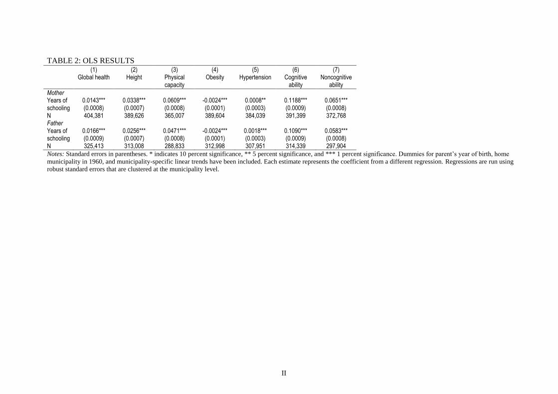
II

TABLE 2: OLS RESULTS (1) (2) (3) (4) (5) (6) (7) Global health Height Physical

capacity Obesity

Hypertension

Cognitive

ability Noncognitive

ability

Mother Years of 0.0143*** 0.0338*** 0.0609*** -0.0024*** 0.0008** 0.1188*** 0.0651*** schooling (0.0008) (0.0007) (0.0008) (0.0001) (0.0003) (0.0009) (0.0008) N 404,381 389,626 365,007 389,604 384,039 391,399 372,768 Father Years of 0.0166*** 0.0256*** 0.0471*** -0.0024*** 0.0018*** 0.1090*** 0.0583*** schooling (0.0009) (0.0007) (0.0008) (0.0001) (0.0003) (0.0009) (0.0008) N 325,413 313,008 288,833 312,998 307,951 314,339 297,904

Notes: Standard errors in parentheses. * indicates 10 percent significance, ** 5 percent significance, and *** 1 percent significance. Dummies for parent’s year of birth, home

municipality in 1960, and municipality-specific linear trends have been included. Each estimate represents the coefficient from a different regression. Regressions are run using

robust standard errors that are clustered at the municipality level.

III

TABLE 3: FIRST STAGE Dependent variable: Education

(A) (B) (C) (D)

Mother Exposed to 0.5557***

(0.0131) 1793.7

405,845

0.2030*** 0.2211*** 0.2528***

reform F-statistic

(0.0586) 12.0

(0.0344) 41.3

(0.0380) 44.2

N 405,845 405,845 405,845 Father Exposed to 0.6645***

(0.0096) 4761.0

326,600

0.2372*** 0.2541*** 0.3539***

reform F-statistic

(0.0795) 8.9

(0.0477) 28.4

(0.0517) 46.8

N 326,600 326,600 326,600 Birth cohort fixed effects

YES YES YES YES

Municipality fixed effects

NO YES YES YES

County-by-year fixed effects

NO NO YES NO

Municipality-specific trends

NO NO NO YES

Notes: Standard errors in parentheses. * indicates 10 percent significance, ** 5 percent significance, and *** 1 percent significance. Each estimate represents the coefficient from

a different regression. Regressions are run using robust standard errors, which in Model B-D are clustered at the municipality level

IV

TABLE 4: IV RESULTS (1) (2) (3) (4) (5) (6) (7) Global

health Height Physical

capacity Obesity

Hypertension

Cognitive

ability Noncognitive

ability

A. Only controlling for birth year fixed effects Mother’s years -0.0294*** 0.0131 0.1047*** -0.0020 0.0270*** 0.0484*** 0.0234** of schooling (0.0105) (0.0104) (0.0107) (0.0016) (0.0042) (0.0100) (0.0107) Father’s years -0.0366*** 0.0171* 0.1119*** -0.0011 0.0199*** 0.0184* 0.0050 of schooling (0.0106) (0.0100) (0.0108) (0.0016) (0.0041) (0.0100) (0.0107)

B. Only controlling for birth year and municipality fixed effects Mother’s years 0.0831* 0.0475 0.1508** -0.0067 0.0956** 0.0893** -0.0138 of schooling (0.0481) (0.0402) (0.0660) (0.0072) (0.0443) (0.0439) (0.0503) Father’s years 0.0016 -0.0252 0.1846** -0.0049 0.0584* -0.0221 -0.0506 of schooling (0.0466) (0.0447) (0.0783) (0.0074) (0.0334) (0.0520) (0.0555) C. Controlling for birth year fixed effects and municipality fixed effects, and interactions between birth year and home county Mother’s years 0.1385*** 0.0796* 0.0164 -0.0103 -0.0023 0.1060** 0.0482 of schooling (0.0507) (0.0454) (0.0476) (0.0072) (0.0182) (0.0416) (0.0471) Father’s years 0.0081 -0.0335 0.0964** -0.0012 0.0259 0.0015 0.0156 of schooling (0.0440) (0.0444) (0.0441) (0.0064) (0.0164) (0.0441) (0.0472) D. Controlling for birth year fixed effects and municipality fixed effects, and municipality-specific trends Mother’s years 0.1031** 0.0888** 0.0182 -0.0071 0.0231 0.1060*** 0.0758* of schooling (0.0464) (0.0424) (0.0437) (0.0068) (0.0176) (0.0384) (0.0450) Father’s years 0.0249 -0.0553 0.0831* -0.0024 0.0177 -0.0372 0.0323 of schooling (0.0407) (0.0365) (0.0429) (0.0059) (0.0143) (0.0419) (0.0429) N (mothers) 404,381 389,626 365,007 389,604 384,039 391,399 372,768 N (fathers) 325,413 313,008 288,833 312,998 307,951 314,339 297,904

Notes: Standard errors in parentheses. * indicates 10 percent significance, ** 5 percent significance, and *** 1 percent significance. Each estimate represents the coefficient from

a different regression. Regressions are run in STATA 12 using the ivregress command and the xtivreg2 command (Schaffer 2010). Regressions are run using robust standard

errors, which in the models in panel B-D are clustered at the municipality level.

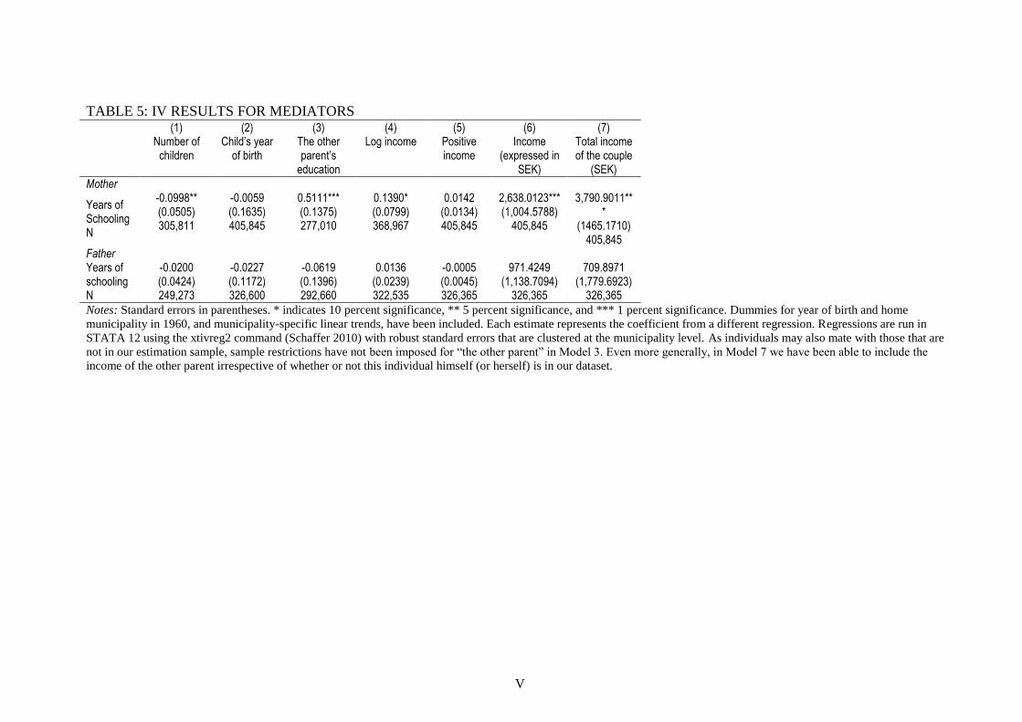
V

TABLE 5: IV RESULTS FOR MEDIATORS (1) (2) (3) (4) (5) (6) (7) Number of

children Child’s year

of birth The other parent’s

education

Log income Positive income

Income (expressed in

SEK)

Total income of the couple

(SEK)

Mother

Years of Schooling N

-0.0998** (0.0505) 305,811

-0.0059 (0.1635) 405,845

0.5111*** (0.1375) 277,010

0.1390* (0.0799) 368,967

0.0142 (0.0134) 405,845

2,638.0123*** (1,004.5788)

405,845

3,790.9011***

(1465.1710) 405,845

Father Years of -0.0200

(0.0424) 249,273

-0.0227 -0.0619 0.0136 -0.0005 971.4249 709.8971 schooling (0.1172) (0.1396) (0.0239) (0.0045) (1,138.7094) (1,779.6923) N 326,600 292,660 322,535 326,365 326,365 326,365

Notes: Standard errors in parentheses. * indicates 10 percent significance, ** 5 percent significance, and *** 1 percent significance. Dummies for year of birth and home

municipality in 1960, and municipality-specific linear trends, have been included. Each estimate represents the coefficient from a different regression. Regressions are run in

STATA 12 using the xtivreg2 command (Schaffer 2010) with robust standard errors that are clustered at the municipality level. As individuals may also mate with those that are

not in our estimation sample, sample restrictions have not been imposed for “the other parent” in Model 3. Even more generally, in Model 7 we have been able to include the

income of the other parent irrespective of whether or not this individual himself (or herself) is in our dataset.

VI

TABLE 6: NINE YEARS OF SCHOOLING AND “SPILL-OVER” EFFECTS At least 9

years of schooling

More than 9 years of schooling

Mother Exposed to reform

0.1048*** (0.0038)

0.0185*** (0.0064)

N 405,845 405,845 Father Exposed to reform

0.1585*** (0.0055)

0.0139* (0.0074)

N 326,600 326,600

Notes: Standard errors in parentheses. * indicates 10 percent significance, ** 5 percent significance, and *** 1 percent significance. Dummies for year of birth and home

municipality in 1960, and municipality-specific linear trends, have been included. Each estimate represents the coefficient from a different regression. Regressions are run using

robust standard errors that are clustered at the municipality level.

VII

TABLE 7: IV RESULTS WHEN EXCLUDING THE MUNICIPALITIES OF STOCKHOLM, GÖTEBORG, AND MALMÖ (1) (2) (3) (4) (5) (6) (7) Global

health Height Physical

capacity Obesity

Hypertension

Cognitive

ability Noncognitive

ability

Mother Years of 0.0853** 0.0872** 0.0345 -0.0079 0.0210 0.1086*** 0.0609 schooling (0.0400) (0.0386) (0.0401) (0.0062) (0.0158) (0.0361) (0.0393) N 362,763 349,407 327,134 349,385 344,819 351,007 333,730 Father Years of 0.0335 -0.0584* 0.0598 -0.0027 0.0181 -0.0134 0.0304 schooling (0.0369) (0.0334) (0.0367) (0.0053) (0.0130) (0.0351) (0.0365) N 292,701 281,415 259,406 281,405 277,281 282,678 267,364

Notes: Standard errors in parentheses. * indicates 10 percent significance, ** 5 percent significance, and *** 1 percent significance. Dummies for parent’s year of birth and home

municipality in 1960, and municipality-specific linear trends have been included. Each estimate represents the coefficient from a different regression. Regressions are run in

STATA 12 using the xtivreg2 command (Schaffer 2010) with robust standard errors that are clustered at the municipality level. The first stage produced a coefficient of 0.2929

and an F-value of 73.8 for mothers and a coefficient of 0.4244 and an F-value of 94.5 for fathers.

VIII

TABLE 8: IV RESULTS WITH COHORT RESTRICTIONS (1) (2) (3) (4) (5) (6) (7) Global

health Height Physical

capacity Obesity

Hypertension

Cognitive

ability Noncognitive

ability

A. Excluding parent individuals born prior to 1943 Mother Years of 0.0901* 0.0899* -0.0065 -0.0049 0.0346 0.1027** 0.0930* schooling (0.0539) (0.0512) (0.0527) (0.0081) (0.0218) (0.0440) (0.0517) N 311,800 299,685 276,710 299,677 294,911 301,029 285,035 Father Years of 0.0112 -0.0365 0.0908* -0.0006 0.0203 -0.0070 0.0247 schooling (0.0511) (0.0484) (0.0550) (0.0077) (0.0169) (0.0437) (0.0478) N 237,336 227,811 206,213 227,808 223,843 228,733 215,381 B. Excluding child individuals born up until 1959 Mother Years of 0.0996** 0.0896** 0.0176 -0.0074 0.0247 0.1061*** 0.0732 schooling (0.0463) (0.0426) (0.0439) (0.0069) (0.0177) (0.0388) (0.0453) N 400,379 385,673 361,055 385,655 380,090 387,440 368,854 Father Years of -0.0263 -0.0550 0.0842** -0.0023 0.0179 -0.0371 0.0334 schooling (0.0407) (0.0365) (0.0423) (0.0059) (0.0142) (0.0417) (0.0426) N 324,846 312,448 288,273 312,438 307,391 313,779 297,351

Notes: Standard errors in parentheses. * indicates 10 percent significance, ** 5 percent significance, and *** 1 percent significance. Dummies for parent’s year of birth and home

municipality in 1960, and municipality-specific linear trends have been included. Each estimate represents the coefficient from a different regression. Regressions are run in

STATA 12 using the xtivreg2 command (Schaffer 2010) with robust standard errors that are clustered at the municipality level. The first stage in panel A produced a coefficient

of 0.2482 and an F-value of 38.9 for mothers and a coefficient of 0.3368 and an F-value of 39.0 for fathers. The first stage in panel B produced a coefficient of 0.2522 and an F-

value of 44.3 for mothers and a coefficient of 0.3545 and an F-value of 47.3 for fathers.