parametric sensitivity and uncertainty analysis of ... · 1506 d. d. lucas and r. g. prinn:...

HAL Id: hal-00295675https://hal.archives-ouvertes.fr/hal-00295675

Submitted on 17 Jun 2005

HAL is a multi-disciplinary open accessarchive for the deposit and dissemination of sci-entific research documents, whether they are pub-lished or not. The documents may come fromteaching and research institutions in France orabroad, or from public or private research centers.

L’archive ouverte pluridisciplinaire HAL, estdestinée au dépôt et à la diffusion de documentsscientifiques de niveau recherche, publiés ou non,émanant des établissements d’enseignement et derecherche français ou étrangers, des laboratoirespublics ou privés.

Parametric sensitivity and uncertainty analysis ofdimethylsulfide oxidation in the clear-sky remote marine

boundary layerD. D. Lucas, R. G. Prinn

To cite this version:D. D. Lucas, R. G. Prinn. Parametric sensitivity and uncertainty analysis of dimethylsulfide oxida-tion in the clear-sky remote marine boundary layer. Atmospheric Chemistry and Physics, EuropeanGeosciences Union, 2005, 5 (6), pp.1505-1525. �hal-00295675�

https://hal.archives-ouvertes.fr/hal-00295675

https://hal.archives-ouvertes.fr

Atmos. Chem. Phys., 5, 1505–1525, 2005www.atmos-chem-phys.org/acp/5/1505/SRef-ID: 1680-7324/acp/2005-5-1505European Geosciences Union

AtmosphericChemistry

and Physics

Parametric sensitivity and uncertainty analysis of dimethylsulfideoxidation in the clear-sky remote marine boundary layer

D. D. Lucas1,* and R. G. Prinn1

1Department of Earth, Atmospheric, and Planetary Sciences, MIT, Cambridge, MA 02139, USA* present address: Frontier Research Center for Global Change, Japan Agency for Marine-Earth Science and Technology,Yokohama, Japan

Received: 18 August 2004 – Published in Atmos. Chem. Phys. Discuss.: 7 October 2004Revised: 2 May 2005 – Accepted: 18 May 2005 – Published: 17 June 2005

Abstract. Local and global sensitivity and uncertainty meth-ods are applied to a box model of the dimethylsulfide (DMS)oxidation cycle in the remote marine boundary layer in orderto determine the key physical and chemical parameters andsources of uncertainty. The model considers 58 uncertain pa-rameters, and simulates the diurnal gas-phase cycles of DMS,SO2, methanesulfonic acid (MSA), and H2SO4 for clear-skysummertime conditions observed over the Southern Ocean.The results of this study depend on many underlying assump-tions, including the DMS mechanism, simulation conditions,and probability distribution functions of the uncertain param-eters. A local direct integration method is used to calculatefirst-order local sensitivity coefficients for infinitesimal per-turbations about the parameter means. Key parameters iden-tified by this analysis are related to DMS emissions, verticalmixing, heterogeneous removal, and the DMS+OH abstrac-tion and addition reactions. MSA and H2SO4 are also sen-sitive to numerous rate constants, which limits the ability ofusing parameterized mechanisms to predict their concentra-tions. Of the chemistry, H2SO4 is highly sensitive to the rateconstants for a set of nighttime reactions that lead to its pro-duction through a non-SO2 path initiated by the oxidation ofDMS by NO3. For the global analysis, the probabilistic col-location method is used to propagate the uncertain parame-ters through the model. The concentrations of DMS and SO2are uncertain (1-σ ) by factors of 3.5 and 2.5, respectively,while MSA and H2SO4 have uncertainty factors that rangebetween 4.1 and 8.6. The main sources of uncertainty inthe four species are from DMS emissions and heterogeneousscavenging, but the uncertain rate constants collectively ac-count for up to 59% of the total uncertainty in MSA and 43%in H2SO4. Of the uncertain DMS chemistry, reactions thatform and destroy CH3S(O)OO and CH3SO3 are identified asimportant targets for reducing the uncertainties.

Correspondence to:D. D. Lucas([email protected])

1 Introduction

The production of dimethylsulfide (CH3SCH3, DMS) by ma-rine phytoplankton (Keller et al., 1989) is believed to bethe largest source of natural sulfur to the global atmosphere(Bates et al., 1992). In the atmosphere DMS is photochemi-cally oxidized to a multitude of sulfur-bearing species, manyof which have an affinity for interacting with existing, or cre-ating new, aerosols. These connections form part of a pro-posed feedback whereby DMS may influence climate andradiation on a planetary scale (Shaw, 1983; Charlson et al.,1987). Although the proposed DMS-climate link has sparkedextensive research (Restelli and Angeletti, 1993; Andreaeand Crutzen, 1997), many large sources of uncertainty stillremain. Two widely used sea-air transfer velocities, for in-stance, yield DMS fluxes that differ by a factor of two (Lissand Merlivat, 1986; Wanninkhof, 1992). As another exam-ple, the formation rates of new sulfate aerosols differ byan order of magnitude between two recent studies (Kulmalaet al., 1998; Verheggen and Mozurkewich, 2002).

Another recognized, but not well quantified, source of un-certainty arises from the gas-phase oxidation of DMS. Theoxidation steps involve many species, competing reactions,and multiple branch points (Yin et al., 1990; Turnipseed andRavishankara, 1993; Urbanski and Wine, 1999; Lucas andPrinn, 2002). Only a small number of the DMS-related rateconstants have been measured in the laboratory, so the ma-jority are estimated (i.e. they are highly uncertain). Quan-tifying the effects of these uncertain chemical reactions onpredictions of the sulfur-containing species is therefore vital.Moreover, it is critical to rank the uncertain DMS chemistryrelative to uncertain non-photochemical processes (e.g. DMSemissions and heterogeneous scavenging). By applying para-metric sensitivity and uncertainty techniques, a quantitativecomparison of these uncertainties is reported here, with thegoal of stimulating further research into the relevant areas.

© 2005 Author(s). This work is licensed under a Creative Commons License.

1506 D. D. Lucas and R. G. Prinn: Sensitivities and uncertainties of DMS oxidation in the RMBL

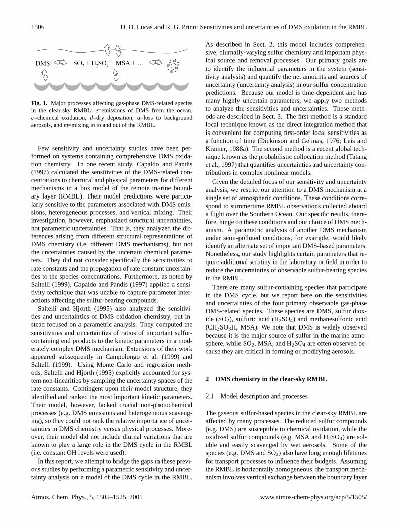
Fig. 1. Major processes affecting gas-phase DMS-related speciesin the clear-sky RMBL:e=emissions of DMS from the ocean,c=chemical oxidation,d=dry deposition,a=loss to backgroundaerosols, andm=mixing in to and out of the RMBL.

Few sensitivity and uncertainty studies have been per-formed on systems containing comprehensive DMS oxida-tion chemistry. In one recent study,Capaldo and Pandis(1997) calculated the sensitivities of the DMS-related con-centrations to chemical and physical parameters for differentmechanisms in a box model of the remote marine bound-ary layer (RMBL). Their model predictions were particu-larly sensitive to the parameters associated with DMS emis-sions, heterogeneous processes, and vertical mixing. Theirinvestigation, however, emphasized structural uncertainties,not parametric uncertainties. That is, they analyzed the dif-ferences arising from different structural representations ofDMS chemistry (i.e. different DMS mechanisms), but notthe uncertainties caused by the uncertain chemical parame-ters. They did not consider specifically the sensitivities torate constants and the propagation of rate constant uncertain-ties to the species concentrations. Furthermore, as noted bySaltelli (1999), Capaldo and Pandis(1997) applied a sensi-tivity technique that was unable to capture parameter inter-actions affecting the sulfur-bearing compounds.

Saltelli and Hjorth (1995) also analyzed the sensitivi-ties and uncertainties of DMS oxidation chemistry, but in-stead focused on a parametric analysis. They computed thesensitivities and uncertainties of ratios of important sulfur-containing end products to the kinetic parameters in a mod-erately complex DMS mechanism. Extensions of their workappeared subsequently inCampolongo et al.(1999) andSaltelli (1999). Using Monte Carlo and regression meth-ods,Saltelli and Hjorth(1995) explicitly accounted for sys-tem non-linearities by sampling the uncertainty spaces of therate constants. Contingent upon their model structure, theyidentified and ranked the most important kinetic parameters.Their model, however, lacked crucial non-photochemicalprocesses (e.g. DMS emissions and heterogeneous scaveng-ing), so they could not rank the relative importance of uncer-tainties in DMS chemistry versus physical processes. More-over, their model did not include diurnal variations that areknown to play a large role in the DMS cycle in the RMBL(i.e. constant OH levels were used).

In this report, we attempt to bridge the gaps in these previ-ous studies by performing a parametric sensitivity and uncer-tainty analysis on a model of the DMS cycle in the RMBL.

As described in Sect.2, this model includes comprehen-sive, diurnally-varying sulfur chemistry and important phys-ical source and removal processes. Our primary goals areto identify the influential parameters in the system (sensi-tivity analysis) and quantify the net amounts and sources ofuncertainty (uncertainty analysis) in our sulfur concentrationpredictions. Because our model is time-dependent and hasmany highly uncertain parameters, we apply two methodsto analyze the sensitivities and uncertainties. These meth-ods are described in Sect.3. The first method is a standardlocal technique known as the direct integration method thatis convenient for computing first-order local sensitivities asa function of time (Dickinson and Gelinas, 1976; Leis andKramer, 1988a). The second method is a recent global tech-nique known as the probabilistic collocation method (Tatanget al., 1997) that quantifies uncertainties and uncertainty con-tributions in complex nonlinear models.

Given the detailed focus of our sensitivity and uncertaintyanalysis, we restrict our attention to a DMS mechanism at asingle set of atmospheric conditions. These conditions corre-spond to summertime RMBL observations collected aboarda flight over the Southern Ocean. Our specific results, there-fore, hinge on these conditions and our choice of DMS mech-anism. A parametric analysis of another DMS mechanismunder semi-polluted conditions, for example, would likelyidentify an alternate set of important DMS-based parameters.Nonetheless, our study highlights certain parameters that re-quire additional scrutiny in the laboratory or field in order toreduce the uncertainties of observable sulfur-bearing speciesin the RMBL.

There are many sulfur-containing species that participatein the DMS cycle, but we report here on the sensitivitiesand uncertainties of the four primary observable gas-phaseDMS-related species. These species are DMS, sulfur diox-ide (SO2), sulfuric acid (H2SO4) and methanesulfonic acid(CH3SO3H, MSA). We note that DMS is widely observedbecause it is the major source of sulfur in the marine atmo-sphere, while SO2, MSA, and H2SO4 are often observed be-cause they are critical in forming or modifying aerosols.

2 DMS chemistry in the clear-sky RMBL

2.1 Model description and processes

The gaseous sulfur-based species in the clear-sky RMBL areaffected by many processes. The reduced sulfur compounds(e.g. DMS) are susceptible to chemical oxidation, while theoxidized sulfur compounds (e.g. MSA and H2SO4) are sol-uble and easily scavenged by wet aerosols. Some of thespecies (e.g. DMS and SO2) also have long enough lifetimesfor transport processes to influence their budgets. Assumingthe RMBL is horizontally homogeneous, the transport mech-anism involves vertical exchange between the boundary layer

Atmos. Chem. Phys., 5, 1505–1525, 2005 www.atmos-chem-phys.org/acp/5/1505/

D. D. Lucas and R. G. Prinn: Sensitivities and uncertainties of DMS oxidation in the RMBL 1507

and overlying free troposphere. Figure1 illustrates these pro-cesses.

The effects of these processes on the sulfur-containingspecies are described by coupled ordinary differential equa-tions (ODEs) of the form

dni

dt= fi(n, pc) − ph,ini + pm(nf,i − ni) + pe,i,

(1)

whereni andnf,i are the gas-phase number concentrationsof sulfur-based speciesi in the RMBL and free troposphere,respectively,f is the net chemical production function, andthe p’s are the process parameters. Specifically,pc repre-sents the set of gas-phase chemical reaction rate constants,ph is the first-order heterogeneous removal parameter,pm

is associated with the parameterized mixing, andpe is theoceanic emissions source. As shown in Table1, our DMSmodel includes 25 sulfur-based species and 58 uncertain pa-rameters (49 gas phase and 9 non-gas phase). The coupledODEs for these 25 species are solved simultaneously usinga stiff ODE solver (i.e. no steady-state approximations areassumed).

As given by Eq. (1), our DMS model is structurally simplebecause it has only four general types of processes (emis-sions, chemistry, heterogeneous removal, and vertical mix-ing). Though structurally simple, we have confidence thatour model adequately describes the essential processes oc-curing in the DMS cycle in the clear-sky RMBL for two rea-sons. First, this model reproduces the general features ofthe boundary layer observations of DMS, SO2, MSA, andH2SO4 analyzed inLucas and Prinn(2002). Second, simi-lar box models have been used to examine field observationsof DMS-related species in the tropical Pacific and SouthernOceans (Davis et al., 1999; Chen et al., 2000; Shon et al.,2001).

The major limitations in Eq. (1) are the lack of cloud pro-cesses and aqueous-phase chemistry. This restricts our studyto clear-sky conditions, but still leaves a rich set of uncer-tainties associated with gas-phase DMS oxidation chemistryand additional non-gas-phase processes. The set of uncer-tainties pertaining to aqueous-phase chemistry and cloud mi-crophysics will require attention in future studies. Anotherlimitation in Eq. (1) involves the use of simple parameters,instead of complex dynamical representations, for the physi-cal processes. We assign reasonable values for these param-eters, however, as described in Sects.2.1.2to 2.1.4. We rec-ognize the shortcomings of this approach, so we also assignlarge uncertainties to these physical parameters.

2.1.1 Gas-phase DMS chemistry

The gas-phase oxidation of DMS is calculated using a mech-anism containing 49 sulfur-containing reactions. In additionto DMS, SO2, MSA, and H2SO4, this mechanism includesdimethylsulfoxide (CH3S(O)CH3, DMSO), dimethylsulfone

(CH3S(O)2CH3, DMSO2), methanesulfenic acid (CH3SOH,MSEA), and methanesulfinic acid (CH3S(O)OH, MSIA).Except for the changes noted later in this section, the reac-tions and rate constants are from the DMS mechanism inLucas and Prinn(2002). The rate constants from that studyhave been set for the conditions of this current study (see Ta-ble 2). This DMS mechanism is ultimately derived from theYin et al. (1990) scheme, but minimized for RMBL condi-tions (e.g. low NOx concentrations and no sulfur-sulfur re-actions). As detailed inLucas and Prinn(2002), the orig-inal Yin et al. (1990) rate constants were updated primar-ily using the recommended values inDeMore et al.(1997),though values were also taken fromAtkinson et al.(1997)and other direct sources. Additional descriptions of this spe-cific DMS mechanism are inLucas(2003) and Lucas andPrinn (2003), while broader reviews of DMS chemistry ingeneral are found inTurnipseed and Ravishankara(1993),Berresheim et al.(1995), andUrbanski and Wine(1999).

Briefly, the DMS oxidation scheme is initialized by reac-tions with OH and NO3, where the former occurs throughtwo independent branches and the latter is potentially impor-tant at night (e.g.Allan et al., 1999). Initialization by halo-gens may also be important (e.g.von Glasow et al., 2002;von Glasow and Crutzen, 2004), but is neglected here dueto poorly-constrained reactive halogen concentrations in theRMBL. Oxidation by OH tends to dominate the net photo-chemical loss of DMS in the RMBL because of the relativelyabundant OH levels and large OH-related rate constants. Tocalculate the nighttime oxidation of DMS by NO3, we in-clude the DMS+NO3 reaction using the rate constant fromDeMore et al.(1997). After the initial oxidation of DMS byOH and NO3, the main oxidants in the mechanism are HOxand O3 because NOx levels are relatively low in the RMBL.Rather than predicting these oxidants directly in our model,we use measurement-based values to enable a specific focuson the sulfur-based chemistry.

As previously mentioned, DMS is oxidized by OH throughtwo independent branches. These are the H-abstraction andOH-addition channels shown below:

CH3SCH3 + OH-add CH3S(OH)CH3

-abs CH3SCH2 + H2O.

The H-abstraction branch is favored at higher temperaturesand leads to the CH3SOx radicals (x=0 to 3), which subse-quently react to form MSA, SO2 and H2SO4 through the gen-eral sequence:

. . . - CH3SO2- CH3SO3

- CH3SO3H

? ?SO2

- SO3- H2SO4.

The key branching points in the above sequence involve theCH3SOx reactions leading to MSA versus the CH3SOx dis-sociations leading to SO2 and H2SO4. The above sequence

www.atmos-chem-phys.org/acp/5/1505/ Atmos. Chem. Phys., 5, 1505–1525, 2005


Table 1. Processes and parameters in the box model of DMS chemistry in the RMBL. The mean values (p) and uncertainty factors (φ) ofthe parameters are listed for the specific conditions of this study (see Table2). For parameter values at other conditions refer toLucas andPrinn(2002). The parameter units are: first-order chemistry, s−1; second-order chemistry, cm3 molecule−1 s−1; heterogeneous loss, s−1;DMS surface emission, molecules cm−3 s−1; and RMBL mixing coefficient, s−1.

Process p φ

Gas-Phase DMS Chemistry

1 CH3SCH3 + OH → CH3SCH2 + H2O 4.85E-12 1.22 CH3SCH3 + NO3 → CH3SCH2 + HNO3 1.1E-12 1.23 CH3SCH3 + OH → CH3S(OH)CH3 3.1E-12 2.04 CH3S(OH)CH3 → CH3SCH3 + OH 2.2E6 2.05 CH3S(OH)CH3 + O2 → CH3S(O)CH3 + HO2 5.0E-13 1.56 CH3S(OH)CH3 → CH3SOH + CH3 5.0E5 3.57 CH3S(O)CH3 + OH → CH3S(O)(OH)CH3 1.0E-10 1.38 CH3S(O)(OH)CH3 + O2 → CH3S(O)2CH3 + HO2 1.0E-13 3.59 CH3S(O)(OH)CH3 → CH3S(O)OH + CH3 2.0E6 3.510 CH3S(O)OH + OH→ CH3SO2 + H2O 9.0E-11 3.511 CH3SCH2 + O2 → CH3SCH2OO 5.7E-12 1.112 CH3SCH2OO + NO→ CH3SCH2O + NO2 1.2E-11 3.513 CH3SCH2O → CH3S + CH2O 3.3E4 3.514 CH3SOH + OH→ CH3SO + H2O 5.0E-11 3.515 CH3SOH + HO2 → CH3SO + H2O2 8.5E-13 3.516 CH3SOH + CH3O2 → CH3SO + CH3O2H 8.5E-13 3.517 CH3S + NO2 → CH3SO + NO 6.4E-11 1.218 CH3S + O3 → CH3SO + O2 5.5E-12 1.219 CH3S + O2 → CH3SOO 3.1E-14 2.020 CH3SOO→ CH3S + O2 1.8E5 2.021 CH3SOO + NO→ CH3SO + NO2 1.1E-11 2.022 CH3SOO + NO2 → CH3SOONO2 2.2E-11 2.023 CH3SOONO2 → CH3SOO + NO2 4.0E-3 3.524 CH3SO + NO2 → CH3SO2 + NO 1.2E-11 1.525 CH3SO + O3 → CH3SO2 + O2 6.0E-13 1.526 CH3SO + O2 → CH3S(O)OO 8.1E-14 3.527 CH3S(O)OO→ CH3SO + O2 4.7E5 3.528 CH3S(O)OO + NO→ CH3SO2 + NO2 8.0E-12 3.529 CH3S(O)OO + NO2 → CH3S(O)OONO2 1.0E-12 3.530 CH3S(O)OONO2 → CH3S(O)OO + NO2 4.2E-3 3.531 CH3SO2 + NO2 → CH3SO3 + NO 2.2E-12 1.532 CH3SO2 + O3 → CH3SO3 + O2 5.0E-15 3.533 CH3SO2 + OH → CH3SO3H 5.0E-11 3.534 CH3SO2 + O2 → CH3S(O)2OO 2.7E-14 3.535 CH3S(O)2OO→ CH3SO2 + O2 1.6E5 3.536 CH3S(O)2OO + NO→ CH3SO3 + NO2 1.0E-11 3.537 CH3S(O)2OO + CH3O2 → CH3SO3 + CH2O + HO2 5.5E-12 3.538 CH3S(O)2OO + NO2 → CH3S(O)2OONO2 1.0E-12 3.539 CH3S(O)2OONO2 → CH3S(O)2OO + NO2 4.2E-3 3.540 CH3SO2 → CH3 + SO2 164 3.541 CH3SO3 → CH3 + SO3 0.16 3.542 CH3SO3 + HO2 → CH3SO3H + O2 5.0E-11 3.543 SO2 + OH → HOSO2 9.2E-13 1.544 HOSO2 + O2 → SO3 + HO2 4.1E-13 1.245 SO3 + H2O → H2SO4 1.6E-13 2.046 CH3SOO→ CH3SO2 1.0 3.547 CH3S(O)OO→ CH3SO3 4.0E-2 3.548 CH3S(O)OH99K CH3SO3H 1.0E-6 3.549 CH3SOH99K CH3SO3H 3.5E-5 3.5Non-Gas-Phase Processes

50 CH3S(O)CH3 → heterogeneous loss 2.0E-4 3.551 CH3S(O)2CH3 → heterogeneous loss 2.0E-4 3.552 CH3SOH→ heterogeneous loss 2.0E-5 3.553 CH3SO2H → heterogeneous loss 2.0E-5 3.554 CH3SO3H → heterogeneous loss 2.5E-4 3.555 SO2 → heterogeneous loss 5.0E-5 3.556 H2SO4 → heterogeneous loss 1.0E-3 3.557 DMS surface emission 9.5E4 3.558 RMBL mixing coefficient 2.5E-5 1.5



also includes a pathway that produces H2SO4 without involv-ing SO2. This pathway has been noted before (Bandy et al.,1992; Lin and Chameides, 1993), but is often assumed to beinefficient due to the relatively fast dissociation of CH3SO2(Kukui et al., 2000) and low levels of CH3SO3. The mech-anism in Table1, however, includes the following reactionsthat enhance CH3SO3 while bypassing CH3SO2:

CH3SO+ O2 CH3S(O)OO - CH3SO3.

The isomerization step above is unique to our mechanism(seeLucas and Prinn, 2002). The net effects of the abovepathway are increases in the levels of MSA and H2SO4 and aslight decrease in the concentration of SO2. The above path-way also increases the production of H2SO4 in the absenceof OH at night after DMS reacts with NO3.

The OH-addition branch of the DMS+OH reaction has anegative temperature-dependence, and is the dominant pathat temperatures below about 275 K. The key branching pointsalong this path occur at OH addition adducts that either re-act with O2 to form DMSO and DMSO2 or dissociate intoMSEA and MSIA. These reactions are summarized below(for x=0 and 1):

CH3S(O)x(OH)CH3

-+O2 CH3S(O)x+1CH3 + HO2

- CH3S(O)xOH + CH3.

The MSEA and MSIA formed in the dissociation branchare rapidly attacked by OH to produce CH3SOx radicals asshown by the following reaction (forx=0 and 1):

CH3S(O)xOH + OH - CH3SOx+1 + H2O.

The resulting CH3SOx radicals can then react or dissociateto form MSA, SO2 and H2SO4 as previously described. Theabove reaction, therefore, serves as a cross-over point fromthe OH-addition branch to the H-abstraction branch. Giventhe potential importance of these reactions, we have updatedthe rate constant for the above MSIA+OH reaction based onnew experimental evidence byKukui et al.(2003). We havealso added two similar reactions (see reactions 15 and 16 inTable1) that convert MSEA to CH3SO by HO2 and CH3O2using the rate constants inYin et al. (1990).

Lastly, we note that the production of MSA is highly un-certain and believed to occur through both the H-abstractionand OH-addition channels. In this model, MSA is explicitlyproduced through the H-abstraction branch by:

CH3SO3 + HO2- CH3SO3H + O2.

In Lucas and Prinn(2002) it was shown that the above re-action alone is not sufficient to produce the levels of MSAobserved in the RMBL, and it was argued that produc-tion through the OH-addition path involving MSEA and/orMSIA is likely. Other studies have suggested similar pro-duction routes (seeHatakeyama and Akimoto, 1983; Koga

and Tanaka, 1993), but the details of these pathways are cur-rently not known. We therefore use the following parameter-ized first-order conversions (represented by dashed arrows)to produce MSA from MSEA and MSIA:

CH3SOH99K 99K CH3SO3H

CH3S(O)OH 99K 99K CH3SO3H.

The paths tested inLucas and Prinn(2002) were used to es-timate the rates of the above first-order, parameterized con-versions.

2.1.2 Heterogeneous removal

Heterogeneous removal is formally estimated usingph=pa+pd , wherepa and pd are loss frequencies due toscavenging by aerosols and dry deposition at the oceansurface, respectively. Scavenging by aerosols dominates thenet heterogeneous removal for most of the DMS oxidationproducts (i.e.ph≈pa). For SO2, however, both losses areimportant. The aerosol loss frequencies (pa) are averagesover the boundary layer portions of the observationally-based vertical scavenging profiles inLucas and Prinn(2002),while the dry deposition losses (pd ) are set using typical drydeposition velocities for a stable RMBL. Theph for SO2 istaken as the empirically-derived removal frequency notedin Lucas and Prinn(2002). The netph values are listed inTable1.

2.1.3 RMBL mixing

Transport into or out of the RMBL is parameterized as theproduct of a first-order mixing coefficient (pm) and the ver-tical concentration difference between the boundary layerand free troposphere (1n). We estimate the mixing co-efficient from the scaling∂/∂z(Kz∂n/∂z)∼pm1n, whereKz is the vertical eddy-diffusion coefficient. This leads topm≈Kz/(1z)2 for a mixing depth scale of1z. The spe-cific mean value ofpm=2.5×10−5 s−1 is estimated fromKz=6.25 m2 s−1 and 1z=500 m, which are representa-tive values for the stable marine atmosphere. The RMBLmixing approximation is applied to DMS, SO2 and MSAbecause these species had large observed vertical gradientsduring the measurement campaign used to define the back-ground conditions in the model (see Sect.2.2). The remain-ing sulfur-containing species are assumed to have no verti-cal concentration gradients. For simplicity and consistency,the free tropospheric concentrations of DMS, SO2 and MSAare fixed in time and based on the observed or modeled val-ues at the interface between the “buffer layer” and free tro-posphere inLucas and Prinn(2002). These values are setas 5.0×107, 2.2×109, and 4.5×106 molecules cm−3, respec-tively, for DMS, SO2 and MSA.



Table 2. Background conditions used in the DMS chemistry model.Each condition is “fixed” or “varies” with time as noted. The valuesare either based on measurements from ACE-1 Flight 24, diagnosedfrom the measurements, or assumed.

Value Time Source

mixed layer depth 500 m fixed measuredtemperature 287 K fixed measuredpressure 980 hPa fixed measuredrelative humidity 75% fixed measuredO3 20 ppb fixed measuredOH see Fig.2 varies measuredHO2, CH3O2, NO2, NO3 see Fig.2 varies diagnosedNO 1 ppt fixed assumed

2.1.4 DMS emissions

DMS emissions are usually calculated using surface windspeeds and DMS sea surface concentrations. For the sakeof simplicity, however, we assume a mean value for theoceanic emission rate ofpe=9.5×104 molecules cm−3 s−1.This emission rate is based on our previous estimate in theRMBL of the Southern Ocean (Lucas and Prinn, 2002). For amixed layer depth of 500 m, the corresponding DMS surfaceflux is comparable to the flux values ofBates et al.(1998b),Mari et al. (1999), andShon et al.(2001). Note that the 2-σ uncertainty range for the DMS emissions parameter ex-tends from 7.8×103 to 1.2×106 molecules cm−3 s−1, whichis larger than the range considered inCapaldo and Pandis(1997) (i.e. 1.0×104 to 1.4×105 molecules cm−3 s−1).

2.2 Background conditions in the RMBL

The background meteorological and oxidizing conditionsused in the box model are given in Table2. These condi-tions are taken from the midpoint of the boundary layer inthe 1-D model ofLucas and Prinn(2002), and are originallybased on the observations from Flight 24 of the First AerosolCharacterization Experiment (ACE-1) (Bates et al., 1998a).The flight occurred during the austral summer in the clear skyover the Southern Ocean southwest of Tasmania. Five-dayback trajectories indicated that the surface air masses wereof a remote marine origin, and the region was characterizedby relatively high DMS concentrations. The measurementswere made between about 05:30 and 14:30 local time (LT),and sunrise and sunset occurred at 04:24 and 19:36 LT, re-spectively.

The important oxidizing-related species OH, O3, H2O2and CH3OOH were measured during the flight. As describedin Lucas and Prinn(2002), the OH and peroxide measure-ments varied with time and were fit to time-dependent “forc-ing” functions. We use the OH forcing function and RMBL-average O3 directly in the model to oxidize the sulfur-basedspecies. The functional fits of the peroxides are used to di-

0 6 12 18 24local time �hours�

108

107

106

105

104

conc

entr

atio

n�m

olec

ules

cm�

3�

�

��

�

�

�

��

�

��

�

�

�

�

�

�

�

�

�

�

�

�

�

�

� OH

� HO2

� CH3O2

� NO2

� NO3

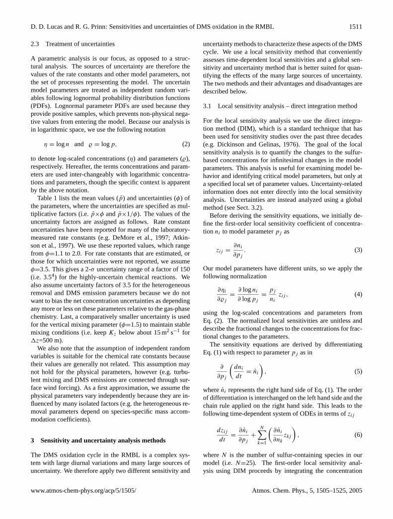
Fig. 2. Diurnal cycles of the radicals used to drive the DMS chem-istry. The OH cycle is based on a fit to measurements and the otherradicals are calculated diagnostically.

agnose the time-dependent concentrations of NO2, HO2, andCH3O2 assuming steady state chemistry.

Two additional oxidants (i.e. NO and NO3) are also re-quired, but were not directly measured during the flight.NO was below the instrument detection limit of 1 ppt, soa constant mole fraction of 1 ppt is assumed. For NO3,Allan et al. (1999) showed that its reaction with DMS isthe primary sink in the summertime RMBL. Therefore, weestimate the time-dependent concentration of NO3 using asteady state balance between production from the NO2+O3reaction and loss by photolysis during the day and by the re-action with DMS at night. These assumptions lead to approx-imate midday and nighttime NO3 concentrations of 6.3×103

and 1.6×106 molecules cm−3, respectively. By comparison,the nighttime NO3 levels used to oxidize DMS byChen et al.(2000) for the remote equatorial Pacific are about three timeslower. The resulting diurnal cycles of OH, HO2, NO2, NO3and CH3O2 are shown in Fig.2.

We emphasize again that our focus is on a detailed sen-sitivity and uncertainty analysis at this single set of RMBLconditions. The conditions within the RMBL are highly vari-able, however, so an analysis at other conditions may yielddifferent results.Capaldo and Pandis(1997), for instance,found important DMS chemistry variations across nine setsof RMBL conditions associated with different locations andseasons. Over their nine scenarios, temperature, O3 and themixing height ranged between 283–300 K, 9–18 ppb, and500–1800 meters, respectively. As an attempt to cover theselarge ranges, we assign relatively large uncertainties to manyof the model parameters. For example, the majority of therate constants have 2-σ uncertainty ranges that are broaderthan their ranges across temperatures of 283 to 300 K. More-over, the 2-σ uncertainty range for DMS emissions is widerthan the emission rates across the nine scenarios inCapaldoand Pandis(1997).



2.3 Treatment of uncertainties

A parametric analysis is our focus, as opposed to a struc-tural analysis. The sources of uncertainty are therefore thevalues of the rate constants and other model parameters, notthe set of processes representing the model. The uncertainmodel parameters are treated as independent random vari-ables following lognormal probability distribution functions(PDFs). Lognormal parameter PDFs are used because theyprovide positive samples, which prevents non-physical nega-tive values from entering the model. Because our analysis isin logarithmic space, we use the following notation

η = logn and % = logp, (2)

to denote log-scaled concentrations (η) and parameters (%),respectively. Hereafter, the terms concentrations and param-eters are used inter-changeably with logarithmic concentra-tions and parameters, though the specific context is apparentby the above notation.

Table1 lists the mean values (p) and uncertainties (φ) ofthe parameters, where the uncertainties are specified as mul-tiplicative factors (i.e.p×φ andp×1/φ). The values of theuncertainty factors are assigned as follows. Rate constantuncertainties have been reported for many of the laboratory-measured rate constants (e.g.DeMore et al., 1997; Atkin-son et al., 1997). We use these reported values, which rangefrom φ=1.1 to 2.0. For rate constants that are estimated, orthose for which uncertainties were not reported, we assumeφ=3.5. This gives a 2-σ uncertainty range of a factor of 150(i.e. 3.54) for the highly-uncertain chemical reactions. Wealso assume uncertainty factors of 3.5 for the heterogeneousremoval and DMS emission parameters because we do notwant to bias the net concentration uncertainties as dependingany more or less on these parameters relative to the gas-phasechemistry. Last, a comparatively smaller uncertainty is usedfor the vertical mixing parameter (φ=1.5) to maintain stablemixing conditions (i.e. keepKz below about 15 m2 s−1 for1z=500 m).

We also note that the assumption of independent randomvariables is suitable for the chemical rate constants becausetheir values are generally not related. This assumption maynot hold for the physical parameters, however (e.g. turbu-lent mixing and DMS emissions are connected through sur-face wind forcing). As a first approximation, we assume thephysical parameters vary independently because they are in-fluenced by many isolated factors (e.g. the heterogeneous re-moval parameters depend on species-specific mass accom-modation coefficients).

3 Sensitivity and uncertainty analysis methods

The DMS oxidation cycle in the RMBL is a complex sys-tem with large diurnal variations and many large sources ofuncertainty. We therefore apply two different sensitivity and

uncertainty methods to characterize these aspects of the DMScycle. We use a local sensitivity method that convenientlyassesses time-dependent local sensitivities and a global sen-sitivity and uncertainty method that is better suited for quan-tifying the effects of the many large sources of uncertainty.The two methods and their advantages and disadvantages aredescribed below.

3.1 Local sensitivity analysis – direct integration method

For the local sensitivity analysis we use the direct integra-tion method (DIM), which is a standard technique that hasbeen used for sensitivity studies over the past three decades(e.g. Dickinson and Gelinas, 1976). The goal of the localsensitivity analysis is to quantify the changes to the sulfur-based concentrations for infinitesimal changes in the modelparameters. This analysis is useful for examining model be-havior and identifying critical model parameters, but only ata specified local set of parameter values. Uncertainty-relatedinformation does not enter directly into the local sensitivityanalysis. Uncertainties are instead analyzed using a globalmethod (see Sect.3.2).

Before deriving the sensitivity equations, we initially de-fine the first-order local sensitivity coefficient of concentra-tion ni to model parameterpj as

zij =∂ni

∂pj

. (3)

Our model parameters have different units, so we apply thefollowing normalization

∂ηi

∂%j

=∂ logni

∂ logpj

=pj

ni

zij , (4)

using the log-scaled concentrations and parameters fromEq. (2). The normalized local sensitivities are unitless anddescribe the fractional changes to the concentrations for frac-tional changes to the parameters.

The sensitivity equations are derived by differentiatingEq. (1) with respect to parameterpj as in

∂

∂pj

(dni

dt= ni

), (5)

whereni represents the right hand side of Eq. (1). The orderof differentiation is interchanged on the left hand side and thechain rule applied on the right hand side. This leads to thefollowing time-dependent system of ODEs in terms ofzij

dzij

dt=

∂ni

∂pj

+

N∑k=1

(∂ni

∂nk

zkj

), (6)

whereN is the number of sulfur-containing species in ourmodel (i.e.N=25). The first-order local sensitivity anal-ysis using DIM proceeds by integrating the concentration



ODEs in Eq. (1) and first-order local sensitivity ODEs inEq. (6). Combined, the first-order local analysis solves for1475 ODEs.

For sensitivity and uncertainty analyses, DIM has twodrawbacks. First, DIM is a local method because a singleDIM run produces sensitivity information at only one set ofpoints in the uncertainty space of the model parameters. Lo-cal sensitivities often vary significantly within the parameteruncertainty space, however, as noted bySaltelli (1999). Thislimits DIM’s effectiveness for estimating model output un-certainties. For example, uncertainties inηi are often extrap-olated from first-order local sensitivities using

σ 2ηi

≈

M∑j=1

(∂ηi

∂%j

)2

σ 2j , (7)

whereσ 2ηi

andσ 2j are the variances ofηi and%j , respectively,

and the summation is overM parameters. We show later inSect.4.2.3that some of the∂ηi/∂%j in our DMS model varyby more than a factor of 2 across the 1-σ uncertainty rangeof parameter%j . For this reason, we do not use DIM in theuncertainty analysis.

As another drawback, DIM is typically restricted to first-order sensitivity studies because higher-order sensitivities,acquired by further differentiation of Eq. (6), lead to largesystems of equations. The second-order sensitivity systemfor our DMS model, for example, has 44 250 ODEs. Becauseinteractions between parameters and other higher-order ef-fects are important in the DMS cycle, higher-order sensitiv-ity coefficients are instead calculated using the global methoddescribed in Sect.3.2.

In spite of these drawbacks, DIM is convenient for analyz-ing local sensitivities as a function of time because Eq. (6)has the same structure as Eq. (1). The same algorithm istherefore used to simultaneously advance the numerical so-lutions to the concentration ODEs and first-order local sen-sitivity ODEs. For this study, we use the Ordinary Differen-tial Equation Solver With Explicit Simultaneous SensitivityAnalysis algorithm fromLeis and Kramer(1988a,b). Thealgorithm is a stiff ODE solver appropriate for models con-taining atmospheric chemistry and it has a built-in capabilityfor performing a first-order local sensitivity analysis.

3.2 Global analysis – probabilistic collocation method

In contrast to the local sensitivity analysis, the global sen-sitivity and uncertainty analysis covers the full uncertaintyranges of the parameters. The primary goals of the globalanalysis are to quantify the net uncertainties in the sulfur-based concentration predictions and to identify and rank theparameter-based contributions to the net uncertainties. To-wards these goals, we utilize the probabilistic collocationmethod (PCM) (Tatang et al., 1997).

PCM is one of many available global methods that quan-tifies and decomposes uncertainties in complex models (e.g.

seeSaltelli et al., 2000). For some models, PCM offers thebenefits of a full Monte Carlo analysis, but at highly-reducedcomputational costs. A detailed description of PCM and itscomparison to the Monte Carlo method are given inTatanget al.(1997). For applications, PCM has been used in uncer-tainty analyses of highly non-linear models of direct and in-direct aerosol radiative forcing (Pan et al., 1997, 1998). PCMhas also been used to create numerically-efficient parameter-izations of non-linear chemical processing in an urban-scalemodel (Calbo et al., 1998; Mayer et al., 2000).

As a brief outline of the methodology, PCM approximatesthe outputs of a model using expansions of orthogonal poly-nomials of the model inputs. The model inputs are cast asrandom variables, where each input parameter is defined bya PDF. The input PDFs serve as weighting functions in re-cursive relationships used to generate the orthogonal poly-nomials, the roots of which are also used to define sets ofcollocation points. The coefficients of the expansions are de-termined by running the model at these sets of collocationpoints. The resulting model output expansions are polyno-mial chaos expansions (PCEs) fit to the true model outputsurface and weighting the high probability regions of themodel inputs. We use the Deterministic Equivalent Mod-eling Method Using Collocation and Monte Carlo package(Tatang, 1995) to construct the orthogonal polynomials, de-termine the collocation points, and perform the numericalfits.

As applied to sensitivity and uncertainty studies, PCM hasnumerous advantages and two disadvantages worth noting.The major advantage is that PCM characterizes the sensitiv-ities and uncertainties throughout the uncertainty domain ofthe model parameters. PCM is thus a global method thatquantifies the contributions of uncertain inputs to the un-certain outputs. Three other advantages are related to thepolynomial representation used by PCM. First, the PCEs arestructured so that the squares of the coefficients are directlyproportional to the variance of the outputs, which makes itstraightforward to identify and rank the sources of uncer-tainty. Second, provided they correlate well with the originalmodel, the PCEs are computationally very efficient versionsof the true model because evaluating polynomials is far moreefficient than, for example, solving ODEs. Third, higher-order analyses, including parameter interactions, are readilyassessable through the coefficients of the higher-order termsin the PCEs (at no additional computational costs).

The following two disadvantages should also be keep inmind in a PCM analysis. PCM can be even more expen-sive than brute-force Monte Carlo for highly non-linear mod-els with many uncertain inputs. Using the DMS model asan example, a full third-order PCE for 58 inputs requires35 990 model runs to fit the coefficients, while a full second-order PCE requires only 1770. Also, to analyze time-varyingmodel outputs, either PCEs must be generated at each time ofinterest or an input random variable for “time” must be intro-duced (e.g. using a uniform PDF). These methods, however,



are cumbersome or difficult for models with very large timevariations.

3.2.1 Application of PCM to the DMS model

The inputs to PCM are the 58 uncertain model parameterslisted in Table1. We use the log-scaled forms of the pa-rameters (i.e.%) and treat them as Gaussian random vari-ables. These are transformed to standard Gaussian randomvariablesξ with a mean of zero and variance of one using

ξk = (%k − %k)/σk, (8)

where%k is thek-th model parameter, and%k andσk are itsmean value and standard deviation. The PDFs ofξk serveas weight functions to generate the orthogonal polynomialbasis for the polynomial chaos expansions. For standard nor-mal PDFs, the corresponding orthogonal polynomials are theHermite polynomials in Table3. As detailed inXiu and Kar-niadakis(2003), different random variables lead to differentorthogonal polynomials used in PCEs (e.g. uniformly dis-tributed random variables correspond with Legendre polyno-mials).

The log-scaled sulfur-containing concentrations are thenexpressed by polynomial chaos expansions of the Hermitepolynomials in terms ofξ . To maintain reasonably-sizedexpansions, the PCEs calculated here include homogeneous(pure) terms up to cubic order and all possible 2nd-orderheterogeneous (cross) terms. The resulting expansions have1828 coefficients. Separate PCEs were generated for DMS,SO2, MSA, and H2SO4. Each PCE has the form (M = 58)

η = α0 +

3∑j=1

M∑k=1

αj,k Hj (ξk)

+

M−1∑k=1

M∑`=k+1

βk,` H1(ξk) H1(ξ`), (9)

whereη approximates the concentration from the true model(i.e. η ≈ η), α0 is the zeroth-order coefficient,αj,k is thej -th order coefficient of thek-th parameter,βk,` is the coef-ficient of the 2nd-order cross term between input parametersk and`, andHj (ξk) is thej -th order Hermite polynomial forthe standard random input parameterξk. The coefficients inEq. (9) are computed from 1828 runs of Eq. (1) at the in-put parameter collocation points, which are chosen from theroots of the Hermite polynomials.

We fit to log-scaled concentrations above for two reasons.First, the solutions to chemical ODEs involve exponentialfunctions, so log-scaling removes much of the exponentialbehavior and allows for better fits with lower-order poly-nomials. Second, lognormally distributed random variablesnaturally result from products of random variables, which arerepresented by the higher-order terms in the PCEs.

Table 3. Hermite polynomials in terms of a standard Gaussian ran-dom variableξ . The expected values of the Hermite polynomialsare also given (see Eq.13 in Sect.3.2.3).

Order Hermite Polynomial E[Hj ] E[H2j] E[H3

j]

0 H0=1 1 1 11 H1=ξ 0 1 02 H2=ξ2

−1 0 2 83 H3=ξ3

−3 ξ 0 6 04 H4=ξ4

−6 ξ2+3 0 24 1728

3.2.2 Local sensitivities using PCM

PCM is a global method, but by differentiating the PCEs withrespect to the model parameters PCM also provides localsensitivity information. This technique is useful for compar-ing the results between PCM and DIM, and for illustratingcertain deficiencies in DIM.

The first-order local sensitivity coefficients using PCM areobtained by differentiating Eq. (9) with respect to%q . Thisyields

∂η

∂%q

σq = α1,q + 2 α2,q ξq + 3 α3,q (ξ2q − 1) +

M∑k=1k 6=q

βk,q ξk,

(10)

whereσq is the standard deviation of%q . We use this ex-pression in two ways. First, we setξ to zero, which givesthe first-order local sensitivities at the parameter means andprovides a way to directly compare to the DIM-based val-ues from Eq. (6). Second, we evaluate Eq. (10) over |ξ |≤1.This analysis shows that many of the first-order local sensi-tivities in the DMS cycle vary dramatically in the parameteruncertainty spaces, and thus using Eq. (7) to extrapolate con-centration uncertainties can lead to large errors.

It is straightforward to derive higher-order local sensitivitycoefficients by further differentiation of Eq. (10). Doing so,the second- and third-order local sensitivity coefficients are

∂2η

∂%2q

σ 2q = 2 α2,q + 6 α3,q ξq ,

∂2η

∂%q∂%r

σqσr = βq,r , and

∂3η

∂%3q

σ 3q = 6 α3,q . (11)

These higher-order local sensitivities are evaluated to gaugethe importance of interactions between model processes andother non-linearities. The presence of large higher-order sen-sitivities signals additional shortcomings in Eq. (7), whichuses only first-order terms to extrapolate concentration un-certainties.

Lastly, the local sensitivities in Eqs. (10) and (11) areweighted by the standard deviations of the parameters. This



implies a relationship between concentrations uncertaintieson the left hand side and the PCE coefficients on the righthand side. This relationship is formally derived in the nextsection by taking the expected values of the PCEs.

3.2.3 Global sensitivities and uncertainties using PCM

The global analysis propagates the uncertain parametersthrough the model and characterizes the statistical propertiesof the uncertain sulfur-containing concentrations. We use thePCEs in Eq. (9) for this analysis. The PCEs could be eval-uated over many random samples of the inputs (i.e.ξ ), thusgenerating concentration PDFs that could then be assessedusing standard statistical methods.

Instead, we extract important statistical properties ofη di-rectly from the PCEs by taking expected values of Eq. (9).The mean value

⟨η⟩, varianceσ 2

η, and skewnessγη, for in-

stance, are determined from⟨η⟩= E[η], σ 2

η= E[(η −

⟨η⟩)2

], and

γη = E[(η −⟨η⟩)3

]/σ 3η, (12)

whereE[ ] denotes an expected value. For multivariaterandom variables, as inη(ξ1, ξ2, . . . ), expected values gen-erally require multidimensional integrations. The expectedvalues ofη, however, are decomposed usingE[aX]=aE[X],E[X+Y ]=E[X]+E[Y ], andE[X Y ]=E[X] E[Y ] for ran-dom variablesX andY and constanta, where the last prop-erty holds for independent variables. The expected values ofEq. (9) therefore simplify into sums and products of

E[Hmj ] =

1√

2π

∫∞

−∞

Hmj (ξ) e−ξ2/2 dξ, (13)

which is the expected value of thej -th order univariate Her-mite polynomial raised to them-th power for a standardGaussian PDF. The relevant values of Eq. (13) are given inTable3.

The mean values of the sulfur-containing concentrationsare derived fromE[η]. Referring to Table3, all of theE[Hj ]

are zero except forE[H0], and so the mean values are simplythe leading coefficients of the PCEs, i.e.⟨

η⟩= α0. (14)

The concentration variances are calculated by taking theexpected value of(η−α0)

2. Using Table3, it is easy toshow that the only non-zero expected values occur for theH 2

j terms. Thus, the variance of Eq. (9) is

σ 2η

=

M∑j=1

(α2

1,j + 2 α22,j + 6 α2

3,j

)+

M−1∑j=1

M∑k=j+1

β2j,k.

(15)

This expression is a quantitative measure of the net uncer-tainties in the sulfur-based concentrations resulting from the

uncertain model parameters. As shown, the net concentrationuncertainties are directly proportional to the squares of thePCE coefficients. This measure also covers the full proba-bilistic space of the uncertain parameters (i.e. Eq.13) and in-cludes higher-order and cross-term contributions. Moreover,the above summations are over parameter indices. Eq. (15)thus provides a quantitative way to allocate the contributionsof the parameter-based sources of uncertainty (i.e. the globalsensitivities). Of the total uncertainty, the uncertainty contri-bution (UC) of parameterq is given by

UCq = α21,q + 2 α2

2,q + 6 α23,q +

M∑k=1k 6=q

β2k,q

2. (16)

Note that the cross term contributionsβ2k,q are divided by two

to evenly split the contribution between the two parametersbecauseξk andξq have the same variance.

Higher-order expected values ofη can also be calculatedusing the same technique, but are increasingly more compli-cated. To illustrate, the skewness of Eq. (9) is obtained fromthe expected value of(η−α0)

3, which results in

γη =1

σ 3η

{M∑

j=1

α2,j

[3 α2

1,j + 8 α22,j + 3

(α1,j + 6 α3,j

)2]

+ 6M−1∑j=1

M∑k=j+1

[βj,k α1,j α1,k + β2

j,k

(α2,j + α2,k

)]

+ 6M−2∑j=1

M−1∑k=j+1

M∑`=k+1

βj,k βj,`βk,`

}. (17)

We use this expression to compute the asymmetries in theconcentrations about their mean values.

4 Results and discussion

The concentrations of the sulfur-containing species aresolved by integrating Eq. (1) for ten days using the stiff ODEsolver. By the final day, repetitive diurnal cycles are achievedfor all of the species. The following analysis is for the finalday of this integration. To provide contrast between periodsof inactive and active chemistry, the global sensitivity anduncertainty analysis using PCM is carried out at 04:00 LT(pre-sunrise) and 12:00 LT (midday).

4.1 Concentrations

4.1.1 Diurnal concentration cycles

The diurnal cycles of DMS, SO2, MSA, and H2SO4 are dis-played in Fig.3 for the mean values of the parameters. Thesesimulated cycles follow the boundary layer observations an-alyzed inLucas and Prinn(2002). The DMS and SO2 cycleshave small amplitudes with peaks shifted away from noon



because they are strongly influenced by non-photochemicalprocesses. The MSA and H2SO4 cycles, on the other hand,have large amplitudes and peak near local noon because theirnet daytime sources are dominated by chemistry. The indi-vidual source and sink terms affecting these concentrationcycles are shown later in Sect.4.2.1.

Also note that the DMS and SO2 cycles are strongly anti-correlated. This anti-correlation has been both observed andmodeled in the RMBL (Davis et al., 1999; Chen et al., 2000),and serves as primary evidence that SO2 in the marine envi-ronment is photochemically produced from DMS oxidation.The phases of the DMS and SO2 cycles in Fig.3 match thecycles modeled for tropical Pacific conditions byDavis et al.(1999) andChen et al.(2000); in particular their maxima andminima occur at roughly the same times. Our diurnal ampli-tudes for DMS and SO2, however, are smaller than inDaviset al. (1999) andChen et al.(2000), due in part to differingstrengths of the OH cycle.

4.1.2 Concentration correlations

PCM is a useful global sensitivity and uncertainty methodonly if the polynomial chaos expansions of the model out-puts are good representations of the true model outputs. Wetest the quality of the PCEs by comparing the concentrationsfrom Eq. (9) with those from Eq. (1) for 103 common setsof randomly sampled parameters. These concentration cor-relations are shown in Fig.4 at 04:00 LT and 12:00 LT. Alsoshown are the 1:1 lines, indices of agreement (d) and coeffi-cients of determination (R2), where theR2 terms denote theamount of variance of the true model captured by the PCEs.

As indicated in the figure, the concentrations from the truemodel and PCEs are highly correlated for the four species.The correlations for MSA and H2SO4 even hold over four tofive orders of magnitude. For a given species, the correlationsare also similar at the two times, except for MSA, which has astronger correlation at 04:00 LT. We are confident, therefore,that the PCEs are good approximations of the true modelbecause they explain essentially all of the variance of DMSand SO2 (97–100%), and significant amounts of the varianceof H2SO4 and MSA (84–91%). The slightly poorer fit forthe PCE of MSA at 12:00 LT, however, impacts some of thesubsequent analysis. This poorer fit is attributed to missingthird-order cross terms involving chemical rate constants inthe PCE.

4.1.3 Concentration polynomial chaos expansions

It is useful to display the polynomial chaos expansions ofthe concentrations directly because much of the subsequentanalysis follows by taking the derivatives and expected val-ues of these PCEs. Table4 shows truncated forms of theconcentration PCEs for DMS, SO2, MSA, and H2SO4. Theleading terms of the expansions in the table are the concen-trations at the mean values of the parameters (i.e. atξ=0).

0 6 12 18 24local time �hours�

107

106

� �

��

��

� �

�

�

�

�

�MSA

�H2 SO4

0 6 12 18 24

109

� ��

��

� ��

��

�

�DMS

�SO2

conc

entr

atio

n�m

olec

ules

cm�

3�

Fig. 3. Diurnal cycles of the concentrations (molecules cm−3) ofDMS, SO2, MSA, and H2SO4 at the mean values of the parameters.

The signs of the PCE coefficients (+/−) indicate whether theconcentrations increase (+) or decrease (−) for increases inthe magnitude of the specified parameter away from its meanvalue. The presence of non-linear terms also signals the po-tential for generating non-symmetric (i.e. skewed) concen-tration PDFs from the PCEs. Even in their truncated forms,the PCEs in Table4 indicate that higher-order terms play animportant role in determining the concentrations. The con-centration of SO2, for instance, depends on non-linear com-binations of heterogeneous removal (ξ55), DMS emissions(ξ57), and RMBL mixing (ξ58). These higher-order termslead to differences in the uncertainties calculated from DIMand PCM.

4.2 Local sensitivity analysis

4.2.1 Diurnal first-order local sensitivity cycles

Figure5 shows the diurnal cycles of the first-order local sen-sitivity coefficients for DMS, SO2, MSA, and H2SO4 derivedfrom Eq. (6) and normalized by Eq. (4). We stress that thesetime-dependent sensitivity cycles are calculated only at themean values of the parameters and do not contain any param-eter uncertainty information. As shown in Sect.4.2.3, thesecycles will change if calculated at other parameter values,and hence are not appropriate for extrapolating concentra-tion uncertainties. Nonetheless, these local sensitivity cyclesare useful for determining the influential source and sink pro-cesses (i.e. positive and negative sensitivities) as a functionof time at the assigned parameter values.



1.3 2.3 3.3 4.3 5.3 6.3 7.3 8.3 9.3

2.5

3.5

4.5

5.5

6.5

7.5

8.5

9.5

10.5

3.7 4.7 5.7 6.7 7.7 8.7 9.7 10.7 11.7

2.5

3.5

4.5

5.5

6.5

7.5

8.5

9.5

10.5log10 �MSA�

R2�0.917d�0.978

R2�0.844d�0.943

0. 1. 2. 3. 4. 5. 6. 7. 8. 9. 10.

1.5

2.5

3.5

4.5

5.5

6.5

7.5

8.5

9.5

10.5

11.5

3. 4. 5. 6. 7. 8. 9. 10. 11. 12. 13.

1.5

2.5

3.5

4.5

5.5

6.5

7.5

8.5

9.5

10.5

11.5log10 �H2 SO4 �

R2�0.906d�0.975

R2�0.904d�0.975

6.75 7.75 8.75 9.75 10.75 11.75

7.5

8.5

9.5

10.5

11.5

12.5

8.25 9.25 10.25 11.25 12.25 13.25

7.5

8.5

9.5

10.5

11.5

12.5log10 �DMS�

R2�1.0d�1.0

R2�1.0d�1.0

6.75 7.75 8.75 9.75 10.75

7.5

8.5

9.5

10.5

11.5

8.25 9.25 10.25 11.25 12.25

7.5

8.5

9.5

10.5

11.5log10 �SO2 �

R2�0.984d�0.996

R2�0.971d�0.992

true model �12:00 LT�

poly

nom

ialc

haos

expa

nsio

ns�0

4:00

LT�

true model �04:00 LT�

poly

nom

ialc

haos

expa

nsio

ns�1

2:00

LT�

Fig. 4. Correlations of the concentrations (log10molecules cm−3) from the true model (Eq.1) and polynomial chaos expansions (Eq.9).Correlations are displayed at 04:00 LT (diamonds, upper/left axes) and 12:00 LT (squares, lower/right axes) using 103 common sets ofparameters sampled randomly from the parameter PDFs. Also shown are the 1:1 lines, coefficients of determination (R2), and indices ofagreement (d).

Table 4. Polynomial chaos expansions of the DMS-related species. The PCEs give the logarithmic concentrations (log10 molecules cm−3)in terms of the standard normal random variablesξk , wherek denotes the parameter number listed in Table1. PCEs are ordered by themagnitudes of the coefficients and are truncated after the seventh largest coefficient.

Time Species Polynomial chaos expansion (log10 molecules cm−3)

04:00 DMS 9.51+0.537ξ57−0.134ξ58+0.010ξ257−0.008ξ3−0.008ξ2

58−0.006ξ1+ . . .

SO2 8.92−0.387ξ55+0.073ξ55 ξ58+0.062ξ57−0.061ξ255+0.060ξ58−0.037ξ57 ξ58+ . . .

MSA 5.77−0.507ξ54+0.145ξ57+0.108ξ58+0.107ξ6−0.086ξ57 ξ58+0.083ξ57 ξ6+ . . .

H2SO4 5.87−0.539ξ56−0.413ξ27+0.405ξ57+0.287ξ47+0.287ξ26−0.134ξ46+ . . .

12:00 DMS 9.45+0.537ξ57−0.138ξ58−0.021ξ3−0.015ξ1+0.010ξ257+0.010ξ4+ . . .

SO2 9.03−0.293ξ55+0.168ξ57−0.086ξ57 ξ58+0.060ξ257−0.059ξ2

55+0.034ξ55 ξ57+ . . .

MSA 6.14−0.407ξ54+0.402ξ57+0.240ξ42+0.217ξ47+0.217ξ26+0.194ξ49+ . . .

H2SO4 6.94−0.516ξ56+0.297ξ57−0.197ξ55−0.189ξ27+0.136ξ47+0.135ξ26+ . . .

As shown, the majority of the local sensitivity coefficientsare extremely time dependent, undergoing rapid changesnear midday and some changes in sign. Though complex,these cycles have the following general features related tothe four types of model processes: (1) The sensitivities to thechemical production and loss rate constants are positive and

negative, respectively, with magnitudes that tend to followphotochemical activity. (2) The sensitivities to the heteroge-neous loss parameters are negative and have their smallestmagnitudes between morning and noon when photochem-istry dominates the concentration changes. (3) The sensitiv-ities to the oceanic DMS source term are positive, but linear



0 6 12 18 24�0.8

�0.6

�0.4

�0.2

0.

0.2

0.4

0.6

0.8

1.DMS

��

��

� � � �

� � � �

� ��

�1

�3

�57

�58

0 6 12 18 24

�0.6

�0.4

�0.2

0.

0.2

0.4

SO2

�

� �

�

�

��

�

�

�

�

�

�

�

�

��1

�55

�57

�58

0 6 12 18 24

�1.

�0.8

�0.6

�0.4

�0.2

0.

0.2

0.4

0.6

0.8MSA

�

� �

�

�

� �

�

�

� �

��

� �

��

� �

�

�

�

� �

�

�

�

�

�

�

�

�

�3

�6

�41

�42

�49

�54

�57

�58

0 6 12 18 24�1.2

�1.

�0.8

�0.6

�0.4

�0.2

0.

0.2

0.4

0.6

0.8

H2 SO4

�

��

�

�

� �

�

�

�

�

�

�

��

�

�

� �

�

�

� �

�

�

� �

�

�

�

��

�

�

�

�

�

�

�

�

�1

�2

�12

�25

�26

�27

�43

47

�56

�57

�58

local time �hours�

�Η��

Fig. 5. Diurnal cycles of the first-order local sensitivity coefficients for the DMS-related species calculated using Eq. (6) and normalizedusing Eq. (4). The “most important” sensitivity coefficients are shown by the dark solid lines with individually labeled symbols and parameternumbers on the right. The most important sensitivities are those with magnitudes within a given threshold of the largest overall value (5%,35%, 28%, and 35% for DMS, SO2, MSA, and H2SO4, respectively). Filled symbols are used for chemical parameters, and empty symbolsare used for heterogeneous removal (empty triangle), DMS emissions (empty square), and RMBL mixing (empty circle). Local sensitivitiesbelow the thresholds are shown using gray-dashed lines. Refer to Table1 for the processes corresponding to the parameter numbers.

for DMS and time varying for the other species. This oc-curs because a change in DMS emissions yields a propor-tional change in the DMS concentration, which then under-goes photochemical oxidation. (4) The sensitivities to thevertical mixing coefficient depend on the sign and magnitudeof the concentration difference between the free troposphereand boundary layer.

In addition to the general features noted above, specificconclusions from Fig.5 for the four species are:

(1) DMS is sensitive to very few parameters. These areprimarily the parameters for oceanic emissions and verticalmixing, although DMS is also moderately sensitive to theDMS+OH abstraction and addition rate constants. The sen-sitivity to the vertical mixing parameter is always negativebecause the concentration of DMS decreases with height.From mid-morning to late afternoon, DMS becomes rela-tively more sensitive to chemistry, due to changes in pho-tochemical activity, and less sensitive to vertical mixing, be-cause of a reduction in the concentration difference betweenthe free troposphere and boundary layer. Interestingly, DMSis not appreciably sensitive to the NO3 oxidation rate con-stant at night, even though the nighttime NO3 concentrationis only 2.2 times lower than the maximum daytime OH con-centration.

(2) SO2 is also sensitive to relatively few parameters.These are the parameters for DMS emissions, vertical mix-ing, heterogeneous removal, and the DMS+OH abstractionrate constant. The sensitivity to the mixing parameter is al-ways positive because SO2 has a larger concentration in thefree troposphere than boundary layer. With time, the sensi-tivity to mixing decreases from its peak value at 08:00 LTto a near-zero value at about 15:00 LT, which coincides with

the lowest and highest SO2 concentrations in Fig.3. Thesedynamical mixing changes are caused by temporal variationsin the SO2 concentration difference between the free tropo-sphere and boundary layer. This difference is large in themorning, because rapid heterogeneous removal and ineffi-cient chemistry reduce the boundary layer levels, and smallin the afternoon, because DMS is chemically oxidized toSO2. Also note that SO2 is always more sensitive to the phys-ical parameters than the rate constants throughout the cycle.Moreover, SO2 is essentially sensitive to only one chemicalrate constant, even though many reactions link SO2 to DMS.

(3) MSA is sensitive to many parameters. The largestsensitivities are associated with DMS emissions, verticalmixing, heterogeneous removal, and the rate constants forDMS+OH addition, MSEA formation, the conversion ofMSEA to MSA, and reactions producing and destroyingCH3SO3. The sensitivity to the vertical mixing parameteris notable in that it is positive at night and negative duringthe day. This change in sign indicates that vertical mixing isa source of boundary layer MSA at night and sink during theday, as driven by changes in the concentration in the bound-ary layer relative to the free troposphere. The sensitivities tothe chemical rate constants also show complex behavior withtime. During the day, MSA is sensitive to the rate constantsfor reactions involving MSEA along the OH-addition chan-nel and CH3SO3 along the H-abstraction channel. At night,MSA retains the sensitivity to the rate constants of some OH-addition reactions, but not any of the H-abstraction reactions.There is also a shift in the relative importance of the OH-addition reactions, which are secondary to DMS emissionsduring the day, but are among the largest positive sensitivi-ties at night.



1 3 6 25 26 27 41 42 47 49 54 57 58�1

�0.5

0

0.5

1

MSA

1 2 19 25 26 27 43 47 55 56 57 58�1

�0.5

0

0.5

1

H2 SO4

1 2 3 4 5 57 58�1

�0.5

0

0.5

1

DMS

1 2 3 12 26 47 55 57 58�0.8�0.6�0.4�0.2

00.20.40.6

SO2

parameter

�Η��

�Η��

DIM �04:00 LT� PCM �04:00 LT� DIM �12:00 LT� PCM �12:00 LT�

Fig. 6. Comparison of the first-order normalized local sensitivity coefficients using DIM (Eqs.6 and4) and PCM (ξ=0 in Eq.10). The localsensitivities are compared at 04:00 LT (DIM gray, PCM white) and 12:00 LT (DIM red, PCM yellow). Refer to Table1 for the parameterlabels.

(4) H2SO4 is sensitive to numerous parameters, includingthose for DMS emissions, heterogeneous removal, and therate constants of many reactions. H2SO4 is also negativelysensitive to the vertical mixing coefficient, even though itsRMBL and free tropospheric concentrations are equal. Asdeduced from the signs of the DMS and SO2 sensitivity coef-ficients to mixing, H2SO4 is affected mainly by the mixing ofDMS, whereby an increase in vertical mixing reduces DMSin the boundary layer and causes a decrease in H2SO4. Thissuggests an important, direct link between DMS and H2SO4that is independent of SO2. This link is more evident in com-paring the sensitivities to the chemical rate constants at dayand night. During the day, H2SO4 is sensitive to the rate con-stants for DMS+OH abstraction, the SO2+OH reaction, andreactions that influence CH3SO and CH3S(O)OO. At night,the OH concentration is low, so the two OH-related sensitivi-ties (i.e. DMS+OH abstraction and SO2+OH) are negligible.The oxidation of DMS by NO3, however, is efficient at night,which leads to CH3SO in the absence of OH. This then ini-tiates the path CH3SO → CH3S(O)OO→ CH3SO3 that isnoted in Sect.2.1.1. The concentration of H2SO4 is thushighly sensitive to these rate constants at night.

Figure5 also shows another interesting feature. Highly-parameterized DMS mechanisms, such as the four reactionschemes inChin et al.(1996) andGondwe et al.(2003), arecommonly used in global models. From the figure, the con-centrations of DMS and SO2 are sensitive to just a few rateconstants, while MSA and H2SO4 are sensitive to many. Thisimplies that highly-parameterized DMS mechanisms are suf-ficient only for oxidizing DMS and forming SO2, not for pro-ducing MSA and H2SO4.

4.2.2 Comparison of first-order local sensitivities

Although PCM is a global method, it still provides local sen-sitivity information at fixed points in the uncertainty spacesof the parameters. Here, we compare the first-order local

sensitivities calculated at the mean values of the parametersusing DIM (Eq.6) and PCM (ξ=0 in Eq.10). The main util-ity in this comparison is to confirm that, at the mean valuesof the parameters, PCM identifies the same set of controllingparameters as identified by DIM. This comparison is shownin Fig. 6 for the largest sensitivities.

As shown in the figure, the DIM and PCM local sensitivitycoefficients are similar in sign and magnitude. This similar-ity even holds over time, as exemplified by the sensitivity ofMSA to the vertical mixing parameter (parameter 58), whichis positive at 04:00 LT and negative at 12:00 LT. The twomethods therefore derive the same general set of critical pa-rameters that influence the chemical concentrations.

Though the overall similarity between DIM and PCM isgood, there are some differences, particularly for H2SO4 andMSA. These differences may result partially from the imper-fect fits between the true model and polynomial chaos expan-sions. However, the concentration correlations in Fig.4 donot show any significant biases towards DIM or PCM. Fur-thermore, some of the local sensitivity differences in Fig.6are larger than the variance differences between the PCEsand true model (i.e. fromR2 in Fig. 4). This suggests thatthe differences are also likely due to the local nature of DIMversus the global/higher-order nature of PCM.

4.2.3 Variations of first-order local sensitivities

The first-order local sensitivity coefficients from DIM pro-vide a reasonable basis for extrapolating uncertainties (seeEq. 7) only if the sensitivities do not vary greatly in the un-certainty spaces of the parameters. This criterion is testedby evaluating Eq. (10). The equation is a multi-dimensionalpolynomial in terms of the model parameters, so we vary theparameters one at a time across their 1-σ uncertainty ranges(i.e. |ξq |≤1), while setting all of the other parameters to theirmean values (i.e.ξk=0 for all k 6=q). Figure7 shows the re-sulting variations at 12:00 LT.



�1 �0.5 0 0.5 10

0.2

0.4

0.6

0.8

1

� � � �

� � ��

��

��

��

�1

�3

�57

�58

DMS

�1 �0.5 0 0.5 10

0.2

0.4

0.6

� � � �

�

�

�

�

�

�

�

�

�

�

�

�

�1

�55

�57

�58

SO2

�1 �0.5 0 0.5 10

0.2

0.4

0.6

0.8

� � � �

�

�

��

�

�

��

��

��

��

�

�

��

��

�

�

�

��

�

�

�

�

�

�

�

��

�1

�3

�6

�26

�42

�47

�49

�54

�57

�58

MSA

�1 �0.5 0 0.5 10

0.2

0.4

0.6

0.8

1

� � � �

�

��

��

��

� � � �

�

�

�

�

�1

�27

�43

�55

56

�57

H2 SO4

��Η� ��

parameter value �Ξ�

Fig. 7. Magnitudes of the first-order normalized local concentration sensitivities at 12:00 LT as the model parameters are varied across their1-σ uncertainty range (−1≤ξ≤1). Only the labeled parameter is varied (ξq ) using Eq. (10) with all other parameters set to their mean values(ξk=0). The sensitivities are displayed and labeled as described in Fig.5 (threshold values of 7%, 20%, 30%, and 30% are used for DMS,SO2, MSA, and H2SO4, respectively).

1st 2nd 2nd�C 3rd 1st 2nd 2nd�C 3rd

0.2

0.4

0.6

0.8

1 54

58

57

58

3 57

57 3 6585858

58

4957

5457

58

54 3 57

57 1 358 3 6

58

2541

MSA


0.2

0.4

0.6

0.8

1 56

2757

182019192518202720

2 5826

56

43

57

574356

574326584743

58

1 25

H2 SO4


0.2

0.4

0.6

0.8

1 57

58

1

58

2 57

13 4585858 58 2 57

57

58

1 58 13

13 35858 4

58 13

DMS


0.2

0.4

0.6

0.8

1

55

58

57

58

552

552 57

585858

58

2 57

55

571

58

5755

57

11

58

5857

58

1 57

SO2

��qΗ� ��

q�

04:00 LT 12:00 LT 04:00 LT 12:00 LT

Fig. 8. Magnitudes of the first-, second-, and third-order normalized local sensitivity coefficients using PCM at 04:00 LT (gray) and 12:00 LT(white). Second-order cross sensitivities are denoted by 2nd-C. Only the three largest magnitudes of each order are shown. The parameternumbers are noted at the top of each bar, andξ is set to zero where applicable. Refer to Table1 for the parameter labels.

From the slopes of the plots in the figure, the magnitudesof many of the local sensitivity coefficients change dramati-cally as the paramters are varied. The sensitivity of SO2 toheterogeneous removal, for example, changes by a factor of2.3 over the 1-σ range of parameter 55. Many of the sensi-tivities for MSA and H2SO4 also experience very large vari-ations. Except for maybe DMS, which has small slopes inFig. 7, we conclude that the local sensitivity coefficients arenot appropriate for estimating the concentration uncertain-ties. The incorrect extrapolation of uncertainties from first-order local sensitivities has been commented on in detail bySaltelli (1999).

There is another interesting feature in Fig.7 pertaining tothe controlling parameters in the DMS cycle. The majorityof the plots in the figure have positive slopes, and the largestslopes are generally related to the physical parameters. Fig-ure 7 therefore shows that the parameters associated withDMS chemistry are relatively more important under condi-

tions of low DMS emissions, weak mixing in the RMBL,and low rates of scavenging by aerosols.

4.2.4 Higher-order local sensitivities

Higher-order local sensitivity coefficients provide a measureof non-linearities and parameter interactions in the DMS sys-tem. Higher-order sensitivities are thus another critical testof the potential for a first-order local analysis using DIM toneglect important and relevant features in sensitivity and un-certainty studies. Figure8 displays the magnitudes of thethree largest first-, second-, and third-order local sensitivitycoefficients using Eqs. (10) and (11).

As shown in the figure, the first-order local sensitivi-ties tend to be larger than the higher-order terms becausethe concentration PCEs are mainly linear in the parame-ters. There are, however, many extremely large second-and third-order sensitivities, particularly for SO2 and MSA.



109108107106105104

0

0.2

0.4

0.6

� �

�

�

�

�

��

�

�

�

�

�

� � � ��

�

�

�

�

�

��

�

�

�

�

�

�

��

�MSA�

109108107106105104103

0

0.1

0.2

0.3

0.4

0.5

0.6

� �

�

�

��

�

�

� ��

�

��

�

�

� � ��

�

�

� �

�

��

�

�

�

�

�

�

� �

�H2 SO4 �

10111010109108

0

0.2

0.4

0.6

0.8

� �

�

�

� �

�

�

� ��

�

�

�

�

�

�

��

�

�

�

�

�

�

��

�

�

�

��

�

�

� �

�DMS�

1010109108107

0

0.2

0.4

0.6

0.8

1

1.2

� � ��

�

�

� �

��

�

�

�

�

�

� ��

�

�

�

�

��

�

�

� �

��

�SO2 �

prob

abili

tyde

nsity

prob

abili

tyde

nsity

04:00 LT � true model � PCEs 12:00 LT � true model � PCEs

Fig. 9. Probability density functions of the DMS-related concentrations (molecules cm−3) using Monte Carlo sampling on the polynomialchaos expansions (PCEs, filled symbols) and true model (empty symbols) at 04:00 LT (diamonds) and 12:00 LT (squares). Sample sizes of104 were used and the PDFs were normalized over 30 equally-spaced bins between the minimum and maximum concentrations.

Upon inspection, the most significant higher-order local sen-sitivities are related to the RMBL mixing parameter. To illus-trate a higher-order effect involving mixing, consider an in-crease in the mixing parameter. This increase reduces DMSin the RMBL, which reduces the amount of SO2 producedfrom the oxidation of DMS, but it also increases the influxof SO2 into the RMBL. Figure8 therefore shows that higher-order processes are important in our DMS model. Becausethe uncertainty estimates from DIM (i.e. Eq.7) neglect thesehigher-order terms, the uncertainty analysis in the next sec-tion uses only PCM.

4.3 Global sensitivity and uncertainty analysis

4.3.1 Statistical properties

Propagating the uncertain parameters through the modelleads to the concentration PDFs of DMS, SO2, MSA, andH2SO4 shown in Fig.9. Two sets of PDFs are comparedin the figure. One set is from Monte Carlo sampling on thetrue model (Eq.1) and the other from sampling the polyno-mial chaos expansions (Eq.9). As shown in the figure, thetwo sets of concentration PDFs have similar characteristics(i.e. shapes and positions). This good comparison thereforesupplies additional support (i.e. in addition to the correla-tions in Sect.4.1.2) that the PCEs adequately represent thetrue model and gives us confidence in using PCM for theglobal analysis. There is a noticeable difference for MSA at12:00 LT, however, in which the PDF from the true model isslightly narrower and shifted to higher concentrations. The

Table 5. Statistical properties of the DMS-related logarithmic con-centrations calculated from the expected values of the polynomialchaos expansions. The values are in units of log10molecules cm−3.

Time Species Mean Variance Skewness

04:00 DMS 9.51 0.30 0.11SO2 8.90 0.17 −0.82MSA 5.84 0.38 0.07H2SO4 5.78 0.87 −0.02

12:00 DMS 9.45 0.30 0.11SO2 9.03 0.16 −0.47MSA 6.25 0.78 0.45H2SO4 6.93 0.51 0.12

slightly poorer fit for MSA at noon is also evident by therelatively lowerR2 value in Fig.4.

Qualitatively from Fig.9, the concentrations of DMS andSO2 are moderately uncertain, while the concentrations ofMSA and H2SO4 are highly uncertain. With time, the mostprobable values for DMS and SO2 are largely invariant, butfor MSA and H2SO4 they shift from lower to higher con-centrations between 04:00 LT and noon. These shifts are re-lated to the amplitudes of the diurnal cycles in Fig.3 relativeto the concentration uncertainties. SO2, for instance, has alarger uncertainty than diurnal amplitude, so the PDFs forSO2 nearly overlap in time.



3 6 26 27 41 42 47 49 54 57 580

102030405060 MSA

19 25 26 27 43 46 47 55 56 57 580

10

20

30

40 H2 SO4

1 3 4 57 580

20

40

60

80 DMS

12 26 27 47 55 57 580

20

40

60

80 SO2

parameter parameter

unce

rtai

nty

cont

ribu

tions�%�

04:00 LT

12:00 LT

Fig. 10. Parameter-based uncertainty contributions (%) for the DMS-related species at 04:00 LT (gray) and 12:00 LT (white). Only thecontributions greater than 0.01%, 0.5%, 1%, and 1% are displayed for DMS, SO2, MSA, and H2SO4, respectively. Refer to Table1 for theparameter labels.

Quantitatively, the mean values of the log-scaled concen-trations using Eq. (14) are listed in Table5. The mean con-centrations using PCM are essentially identical to those oftrue model (not shown in the table) except for MSA at noon(i.e. true model≈6.38). This implies that theα0 coefficientsof the PCEs are excellent estimators of the mean values. Itis also useful to compare the mean values in Table5 with theleading coefficients in Table4, where the latter equal the log-scaled concentrations at the mean values of the parameters(i.e. ξ=0). Of the two sets of values, there is good corre-spondence only for DMS. This indicates a sufficient degreeof nonlinearity such that running the model at the mean val-ues of the parameters does not give good estimates for themean values of the concentrations.

An important part of the global analysis is to quantify thenet uncertainties in the sulfur-bearing concentrations. Thenet uncertainties are associated with the variances, which arecalculated by Eq. (15) and listed in Table5. As with themean values, the variances of the PCEs are nearly equal tothose of the true model (not shown), except for MSA at noon(i.e. true model≈0.52). To quantify the concentration uncer-tainties, the variances are converted to uncertainty factors (φ)using log10φ=ση. This conversion shows that the concentra-tions of DMS and SO2 are uncertain by factors of approxi-mately 3.5 and 2.5, respectively, while MSA and H2SO4 areuncertain by factors ranging between about 4.1 to 8.6. Inter-estingly, SO2 is less uncertain than DMS, even though SO2 isproduced by an extensive set of uncertain chemical reactions.This occurs because SO2 is also less sensitive to the modelparameters (e.g. see Fig.6). Another interesting feature isthat the uncertainty of H2SO4 is larger at night than midday,even though the overall chemical activity is lower. This re-sults from the enhanced sensitivity of H2SO4 to productionthrough the highly-uncertain non-SO2 pathway at night (e.g.see Fig.5).

The concentration skewness values using Eq. (17) are alsolisted in Table5. These values are listed mainly for qualita-tive reasons because skewness estimates are less robust thanestimates of lower-order statistical moments. The skewnessvalues nonetheless confirm that the SO2 concentration PDFsshown in Fig.9 have long tails to the left of the mean val-ues. Using PCM, the sources of SO2 asymmetry can be as-certained from the magnitudes of the higher-order terms inthe PCEs because, from the central limit theorem, sums andproducts of independent random variables tend towards nor-mal (symmetric) and lognormal (asymmetric) distributions,respectively. Referring to Table4, the PDFs of SO2 areasymmetric primarily because of combinations of the pa-rameters for heterogeneous removal, DMS emissions, andRMBL mixing.

4.3.2 Uncertainty contributions

The second major goal of the global analysis is to partitionthe net concentration uncertainties into contributions fromthe uncertain parameters. This is done on a per parameterbasis using Eq. (16), which includes contributions from pairsof uncertain parameters. The results are displayed in Fig.10.First note the contrast between Figs.6 and10, which high-lights the important distinction between the local sensitiv-ity analysis and global uncertainty analysis. Fig.6 showsthat SO2 is locally sensitive to the DMS+OH abstraction rateconstant, yet Fig.10 indicates that this parameter makes anegligible contribution to the uncertainty in SO2.

Fig. 10serves as a useful guide for reducing the uncertain-ties in the concentrations of DMS, SO2, MSA, and H2SO4.It is clear from the figure that better constraints on the pa-rameters associated with DMS emissions (parameter 57) andheterogeneous removal (parameters 50–56) will go a longway towards reducing the overall concentration uncertain-ties. Other important general conclusions from the figure areas follows:



Table 6. Percent contributions to the concentration variances fromchemical and physical parameters and cross terms.

Time Species Parameters Cross terms

Chemical Physical

04:00 DMS 0 100 0SO2 1 99 4MSA 14 86 14

H2SO4 43 57 5

12:00 DMS 0 100 0SO2 4 96 8MSA 59 41 23

H2SO4 25 75 14

– The uncertainty in DMS emissions contributes morethan 90% to the uncertainty in DMS, but only 5–30%to the other species. Better knowledge of DMS emis-sions alone, therefore, will only reduce the uncertaintiesof the oxidized sulfur compounds by moderate levels.

– The uncertainties in DMS and SO2 are caused by just afew physical parameters. MSA and H2SO4, in contrast,have uncertainty contributions from many chemical andphysical parameters. This implies that it should be rel-atively easier to reduce the uncertainties in DMS andSO2, than in MSA and H2SO4.

– The uncertain heterogeneous removal parameters arethe primary sources of uncertainty in SO2 and H2SO4at night and day, and in MSA at night.

– The initial DMS oxidation rate constants involving OHand NO3 do not contribute significantly to the concen-tration uncertainties because they are relatively well un-derstood (i.e. have low parameter uncertainties).

– Although chemical parameters are not the dominantsources of uncertainty, the rate constants associatedwith the formation and loss of CH3S(O)OO make siz-able contributions to the uncertainties in H2SO4 at nightand MSA during the day.

– For H2SO4, there are uncertainty contributions from therate constants for the isomerization of CH3SOO at nightand SO2+OH reaction at noon. For MSA, notable rateconstant contributions originate from midday reactionsinvolving MSEA and CH3SO3.

– The uncertainty contributions change in time for thenon-DMS species, with the most dramatic changes oc-curing for MSA. At night MSA has essentially no un-certainty contributions from chemical parameters, butat noon nearly 50% of the net uncertainty in MSA is

attributed to eight rate constants. Many of these tem-poral changes are related to the diurnal local sensitivityprofiles in Fig.5.

– In contrast toSaltelli and Hjorth(1995), the uncer-tainty contributions from the dissociation rate constantof CH3SO2 are insignificant, even though this pathwaydirectly forms SO2 and H2SO4. This discrepancy arisesbecause our DMS model contains non-photochemicalprocesses and additional chemical pathways formingSO2 and H2SO4.

It is difficult to gauge from Fig.10 the net impact of theuncertain chemistry because the chemical contributions arespread over a large number of parameters. Using Eq. (16),the contributions from the chemical parameters (1–49) andphysical parameters (50–58) are summed up separately anddisplayed in Table6. As noted in the table, uncertain physi-cal parameters account for practically all of the uncertainty inDMS and SO2. The aggregated chemical parameters, how-ever, comprise up to 43% and 59% of the total uncertainty inH2SO4 and MSA, respectively. This implies that to achievesignificant reductions in the net uncertainties of the oxidizedDMS products, a better understanding of many reactions inthe DMS mechanism is required. Moreover, the total contri-bution from pairs of uncertain parameters (i.e. theβ2 terms inEq.15) are summed up and displayed in Table6. This analy-sis indicates that pairs of parameters account for up to 8% ofthe total uncertainty in SO2, up to 23% in MSA, and as muchas 14% in H2SO4. As a result, efforts to reduce the uncer-tainties in the DMS-related concentrations should also seekto gain a better understanding of the interactions between thevarious processes.

5 Conclusions

A box model of the diurnal cycle of DMS in the clear-skyremote marine boundary layer is applied to a set of sum-mertime, mid-latitude conditions observed over the SouthernOcean. The rate constants and physical parameters in themodel are treated as sources of uncertainty, and the sensi-tivities and uncertainties of the gas-phase concentrations ofDMS, SO2, MSA, and H2SO4 are analyzed.

A direct integration method is used to calculate the diur-nal cycles of the first-order local sensitivity coefficients forinfinitesimal perturbations about the mean values of the pa-rameters. From this local analysis, the sulfur-bearing com-pounds are found to be especially sensitive to the parame-ters associated with DMS emissions, mixing with the freetroposphere, heterogeneous removal, and the DMS+OH ad-dition and abstraction reactions. The largest overall localsensitivity coefficients are related to the physical parame-ters, not the chemical rate constants. The concentrationsof MSA and H2SO4, however, are appreciably sensitive tonumerous rate constants beyond the initial reactions in the



DMS oxidation mechanism. This implies that many of thehighly-parameterized DMS mechanisms employed in large-scale models are likely missing key features of DMS chem-istry. Large temporal variations are also observed for thecomputed first-order local sensitivity coefficients, particu-larly for H2SO4. At night, sulfuric acid is much more sensi-tive to the rate constants for a sequence of reactions initiatedby DMS+NO3 and leading to CH3SO3. These reactions de-serve future attention because, for sufficient levels of NO3,they enhance the nighttime production of H2SO4 in the ab-sence of SO2 and OH.

The probabilistic collocation method is used to propagatethe uncertain rate constants and physical parameters throughthe DMS model. PCM is a global sensitivity and uncertaintymethod that quantifies the net amounts and sources of un-certainty. From this analysis, the concentrations of DMSand SO2 are uncertain (1-σ ) by factors of roughly 3.5 and2.5, respectively. SO2 is less uncertain than DMS becauseit is also less sensitive to the model parameters. MSA andH2SO4 have concentration uncertainties that vary with timeand range between factors of 4.1 to 8.6. MSA is found to bemore uncertain at midday due to additional production pathsthat are active during the day. H2SO4, however, is moreuncertain at night because of heightened sensitivities to thenighttime production through a non-SO2 pathway.

The global PCM analysis also identifies the parameter-based sources of uncertainty in the DMS-related compounds.Although all of the compounds are locally sensitive to theDMS+OH abstraction rate constant, this parameter does notmake significant uncertainty contributions because it is rela-tively well known. We instead find that the uncertainties inthe concentrations are caused predominantly by the uncertainparameters for DMS emissions and heterogeneous scaveng-ing. We recommend that field studies of the DMS cycle inthe remote marine boundary layer attempt to quantify theseprocesses so as to reduce the overall uncertainties.

For MSA and H2SO4, however, we also find that many in-dividual uncertain rate constants contribute at a 5% or higherlevel. Collectively, the uncertain rate constants account forup to 59% and 43% of the total uncertainty in MSA andH2SO4, respectively. To achieve substantial reductions inthe uncertainties of these two species will therefore requirebetter knowledge of many reactions in the DMS oxidationmechanism. Of the many reactions, our uncertainty analy-sis suggests initially targeting those reactions associated withthe formation and loss of CH3S(O)OO and CH3SO3, whichmay help to reduce the uncertainties in H2SO4 at night andMSA during the day.

Acknowledgements.We are grateful to A. Saltelli and the fouranonymous reviewers for their many helpful comments. This workwas supported by NASA grant NAG5-12099 and the federal andindustrial sponsors of the MIT Joint Program on the Science andPolicy of Global Change.

Edited by: N. Mihalopoulos

References

Allan, B. J., Carslaw, N., Coe, H., Burgess, R. A., and Plane,J. M. C.: Observations of the Nitrate Radical in the MarineBoundary Layer, J. Atmos. Chem., 33, 129–154, 1999.

Andreae, M. and Crutzen, P.: Atmospheric Aerosols: Biogeochem-ical Sources and Role in Atmospheric Chemistry, Science, 276,1052–1058, 1997.

Atkinson, R., Baulch, D. L., Cox, R. A., Hampson, R., Kerr, J. A.,Rossi, M. J., and Troe, J.: Evaluated Kinetic and Photochemi-cal Data for Atmospheric Chemistry: Supplement VI, J. Phys.Chem. Ref. Data, 26, 1329–1499, 1997.

Bandy, A. R., Scott, D. L., Blomquist, B. W., Chen, S. M., andThorton, D. C.: Low Yields of SO2 from Dimethyl Sulfide Ox-idation in the Marine Boundary Layer, Geophys. Res. Lett., 19,1125–1127, 1992.

Bates, T. S., Lamb, B. K., Guenther, A., Dignon, J., and Stoiber,R. E.: Sulfur Emissions to the Atmosphere from Natural Sources,J. Atmos. Chem., 14, 315–337, 1992.

Bates, T. S., Huebert, B., Gras, J., Griffiths, F., and Durkee, P.: TheInternational Global Atmospheric Chemistry (IGAC) Project’sFirst Aerosol Characterization Experiment (ACE 1): Overview,J. Geophys. Res., 103, 16 297–16 318, 1998a.

Bates, T. S., Kapustin, V. N., Quinn, P. K., Covert, D. S., Coffman,D. J., Mari, C., Durkee, P. A., De Bruyn, W. J., and Saltzman,E. S.: Processes controlling the distribution of aerosol particles inthe lower marine boundary layer during the First Aerosol Char-acterization Experiment (ACE 1), J. Geophys. Res., 103, 16 369–16 383, 1998b.

Berresheim, H., Wine, P. H., and Davis, D. D.: Sulfur in the At-mosphere, in: Composition, Chemistry, and Climate of the At-mosphere, edited by: Singh, H. B., pp. 251–307, Van NostrandReinhold, New York, 1995.

Calbo, J., Pan, W., Webster, M., Prinn, R., and McRae, G.: Param-eterization of Urban Sub-Grid Scale Processes in Global Atmo-spheric Chemistry Models, J. Geophys. Res., 103, 3437–3452,1998.

Campolongo, F., Saltelli, A., Jensen, N. R., Wilson, J., and Hjorth,J.: The Role of Multiphase Chemistry in the Oxidation ofDimethylsulphide (DMS), A Latitude Dependent Study, J. At-mos. Chem., 32, 327–356, 1999.

Capaldo, K. P. and Pandis, S. N.: Dimethylsulfide Chemistry in theRemote Marine Atmosphere: Evaluation and Sensitivity Anal-ysis of Available Mechanisms, J. Geophys. Res., 102, 23 251–23 267, 1997.

Charlson, R., Lovelock, J., Andreae, M., and Warren, S.: OceanicPhytoplankton, Atmospheric Sulphur, Cloud Albedo, and Cli-mate, Nature, 326, 655–661, 1987.

Chen, G., Davis, D. D., Kasibhatla, P., Bandy, A. R., Thornton,D. C., Huebert, B. J., Clarke, A. D., and Blomquist, B. W.: AStudy of DMS Oxidation in the Tropics: Comparison of Christ-mas Island Field Observations of DMS, SO2, and DMSO withModel Simulations, J. Atmos. Chem., 37, 137–160, 2000.

Chin, M., Jacob, D. J., Gardner, G. M., Foreman-Fowler, M. S.,Spiro, P. A., and Savoie, D. L.: A Global Three-DimensionalModel of Tropospheric Sulfate, J. Geophys. Res., 101, 18 667–18 690, 1996.

Davis, D., Chen, G., Bandy, A., Thornton, D., Eisele, F., Mauldin,L., Tanner, D., Lenschow, D., Fuelberg, H., Huebert, B., Heath,J., Clarke, A., and Blake, D.: Dimethyl Sulfide Oxidation in the



Equatorial Pacific: Comparison of Model Simulations with FieldObservations for DMS, SO2, H2SO4(g), MSA(g), MS, and NSS,J. Geophys. Res., 104, 5765–5784, 1999.

DeMore, W., Sander, S., Golden, D., Hampson, R., Howard, C.,Ravishankara, A., Kolb, C., and Molina, M.: Chemical Kinet-ics and Photochemical Data for Use in Stratospheric Modeling,Tech. Rep. Evaluation No. 12, Jet Propulsion Laboratory, NASA,Pasadena, CA, 1997.

Dickinson, R. P. and Gelinas, R. J.: Sensitivity Analysis of Ordi-nary Differential Equation Systems – A Direct Method, J. Comp.Phys., 21, 123–143, 1976.

Gondwe, M., Krol, M., Gieskes, W., Klaassen, W., and de Baar, H.:The Contribution of Ocean-Leaving DMS to the Global Atmo-spheric Burdens of DMS, MSA, SO2, and NSS SO=4 , GlobalBiogeochem. Cycles, 17, 1056, doi:10.1029/2002GB001937,2003.

Hatakeyama, S. and Akimoto, H.: Reactions of OH radicals withmethanethiol, dimethyl sulfide, and dimethyl disulfide in air, J.Phys. Chem., 87, 2387–2395, 1983.

Keller, M., Bellows, W., and Guillard, R.: Dimethylsulfide Produc-tion in Marine Phytoplankton, in: Biogenic Sulfur in the Envi-ronment, edited by: Saltzman, E. and Cooper, W., pp. 167–182,American Chemical Society, Washington, D.C., 1989.

Koga, S. and Tanaka, H.: Numerical study of the oxidation processof dimethylsulfide in the marine atmosphere, J. Atmos. Chem.,17, 201–228, 1993.

Kukui, A., Bossoutrot, V., Laverdet, G., and Le Bras, G.: Mecha-nism of the Reaction of CH3SO With NO2 in Relation to Atmo-spheric Oxidation of Dimethyl Sulfide: Experimental and Theo-retical Study, J. Phys. Chem. A, 104, 935–946, 2000.

Kukui, A., Borissenko, D., Laverdet, G., and Le Bras, G.: Gas-Phase Reactions of OH Radicals with Dimethyl Sulfoxide andMethane Sulfinic Acid Using Turbulent Flow Reactor and Chem-ical Ionization Mass Spectrometry, J. Phys. Chem. A, 107, 5732–5742, 2003.

Kulmala, M., Laaksonen, A., and Pirjola, L.: Parameterizations forSulfuric Acid/Water Nucleation Rates, J. Geophys. Res., 103,8301–8307, 1998.

Leis, J. R. and Kramer, M. A.: The Simultaneous Solution and Sen-sitivity Analysis of Systems Described by Ordinary DifferentialEquations, ACM Trans. Math. Software, 14, 45–60, 1988a.

Leis, J. R. and Kramer, M. A.: Algorithm 658: ODESSA – An Or-dinary Differential Equation Solver With Explicit SimultaneousSensitivity Analysis, ACM Trans. Math. Software, 14, 61–67,1988b.

Lin, X. and Chameides, W. L.: CCN Formation From DMS Ox-idation Without SO2 Acting as an Intermediate, Geophys. Res.Lett., 20, 579–582, 1993.

Liss, P. S. and Merlivat, L.: Air-sea gas exchange rates: Introductionand synthesis, in: The Role of Air-Sea Exchange in GeochemicalCycling, edited by: Buat-Menard, P. and Reidel, D., pp. 113-127,Norwell, Mass, 1986.

Lucas, D. D.: Mechanistic, Sensitivity, and Uncertainty Studiesof the Atmospheric Oxidation of Dimethylsulfide, Ph.D. thesis,Massachusetts Institute of Technology, Cambridge, MA, Centerfor Global Change Science Report 71,http://web.mit.edu/cgcs/www/MIT CGCSRpt71.html, 2003.

Lucas, D. D. and Prinn, R. G.: Mechanistic Studies ofDimethylsulfide Oxidation Products Using an Observation-

ally Constrained Model, J. Geophys. Res., 107, 4201,doi:10.1029/2001JD000843, 2002.

Lucas, D. D. and Prinn, R. G.: Tropospheric distributionsof sulfuric acid-water vapor aerosol nucleation rates fromdimethylsulfide oxidation, Geophys. Res. Lett., 30, 2136,doi:10.1029/2003GL018370, 2003.

Mari, C., Suhre, K., Rosset, R., Bates, T. S., Huebert, B. J., Bandy,A. R., Thorton, D. C., and Businger, S.: One-Dimensional Mod-eling of Sulfur Species During the First Aerosol Characteriza-tion Experiment (ACE 1) Lagrangian B, J. Geophys. Res., 104,21 733–21 749, 1999.

Mayer, M., Wang, C., Webster, M., and Prinn, R. G.: Linking LocalAir Pollution to Global Chemistry and Climate, J. Geophys. Res.,105, 22 869–22 896, 2000.

Pan, W., Tatang, M., McRae, G., and Prinn, R.: UncertaintyAnalysis of Direct Radiative Forcing by Anthropogenic SulfateAerosols, J. Geophys. Res., 102, 21 915–21 924, 1997.

Pan, W., Tatang, M., McRae, G., and Prinn, R.: UncertaintyAnalysis of Indirect Radiative Forcing by Anthropogenic SulfateAerosols, J. Geophys. Res., 103, 3815–3824, 1998.

Restelli, G. and Angeletti, G. (Eds.): Dimethylsulphide: Oceans,Atmosphere, and Climate, Kluwer, Dordrecht, Netherlands,1993.

Saltelli, A.: Sensitivity Analysis: Could Better Methods Be Used?,J. Geophys. Res., 104, 3789–3793, 1999.

Saltelli, A., Chan, K., and Scott, E. M. (Eds.): Sensitivity Analysis,John Wiley and Sons, New York, 2000.

Saltelli, A. and Hjorth, J.: Uncertainty and Sensitivity Analyses ofOH-Initiated Dimethyl Sulphide (DMS) Oxidation Kinetics, J.Atmos. Chem., 21, 187–221, 1995.

Shaw, G.: Bio-Controlled Thermostasis Involving the Sulfur Cycle,Climatic Change, 5, 297–303, 1983.

Shon, Z., Davis, D., Chen, G., Grodzinsky, G., Bandy, A., Thor-ton, D., Sandholm, S., Bradshaw, J., Stickel, R., Chameides, W.,Kok, G., Russell, L., Mauldin, L., Tanner, D., and Eisele, F.:Evaluation of the DMS Flux and its Conversion to SO2 over theSouthern Ocean, Atmos. Environ., 35, 159–172, 2001.

Tatang, M.: Direct Incorporation of Uncertainty in Chemical andEnvironmental Engineering Systems, Ph.D. thesis, MIT, Cam-bridge, MA, 1995.

Tatang, M., Pan, W., Prinn, R., and McRae, G.: An Efficient Methodfor Parametric Uncertainty Analysis of Numerical GeophysicalModels, J. Geophys. Res., 102, 21 925–21 932, 1997.

Turnipseed, A. A. and Ravishankara, A. R.: The Atmospheric Ox-idation of Dimethyl Sulfide: Elementary Steps in a ComplexMechanism, in: Dimethylsulphide: Oceans, Atmospheres, andClimate, edited by: Restelli, G. and Angeletti, G., pp. 185–195,Kluwer, Dordrecht, 1993.

Urbanski, S. P. and Wine, P. H.: Chemistry of Gas Phase OrganicSulfur-Centered Radicals, in: S-Centered Radicals, edited by:Alfassi, Z. B., pp. 97–140, Wiley, Chichester, 1999.

Verheggen, B. and Mozurkewich, M.: Determination of Nucle-ation and Growth Rates from Observations of a SO2 InducedAtmospheric Nucleation Event, J. Geophys. Res., 107, 4123,doi:10.1029/2001JD000683, 2002.

von Glasow, R., Sander, R., Bott, A., and Crutzen, P. J.: ModelingHalogen Chemistry in the Marine Boudary Layer 2. InteractionsWith Sulfur and the Cloud-Covered MBL, J. Geophys. Res., 107,4323, doi:10.1029/2001JD000943, 2002.


http://web.mit.edu/cgcs/www/MIT_CGCS_Rpt71.html

http://web.mit.edu/cgcs/www/MIT_CGCS_Rpt71.html


von Glasow, R. and Crutzen, P. J.: Model Study of Multiphase DMSOxidation With a Focus on Halogens, Atmos. Chem. Phys., 4,589–608, 2004,SRef-ID: 1680-7324/acp/2004-4-589.

Wanninkhof, R.: Relationship Between Wind Speed and Gas Ex-change over the Ocean, J. Geophys. Res., 97, 7373–7382, 1992.

Xiu, D. and Karniadakis, G. E.: Modeling uncertainty in flow simu-lations via generalized polynomial chaos, J. Comput. Phys., 187,137–167, doi:10.1016/S0021-9991(03)00092-5, 2003.

Yin, F., Grosjean, D., and Seinfeld, J.: Photooxidation of DimethylSulfide and Dimethyl Disulfide. I. Mechanism Development, J.Atmos. Chem., 11, 309–364, 1990.


http://direct.sref.org/1680-7324/acp/2004-4-589

parametric sensitivity and uncertainty analysis of ... · 1506 d. d. lucas and r. g. prinn:...

Documents