parametric image alignment using enhanced correlation coefficient maximization

Short Papers__________________________________________________________________________________________________

Parametric Image Alignment Using EnhancedCorrelation Coefficient Maximization

Georgios D. Evangelidis andEmmanouil Z. Psarakis

Abstract—In this work, we propose the use of a modified version of the

correlation coefficient as a performance criterion for the image alignment problem.

The proposed modification has the desirable characteristic of being invariant with

respect to photometric distortions. Since the resulting similarity measure is a

nonlinear function of the warp parameters, we develop two iterative schemes for

its maximization, one based on the forward additive approach and the second on

the inverse compositional method. As is customary in iterative optimization, in

each iteration, the nonlinear objective function is approximated by an alternative

expression for which the corresponding optimization is simple. In our case, we

propose an efficient approximation that leads to a closed-form solution (per

iteration) which is of low computational complexity, the latter property being

particularly strong in our inverse version. The proposed schemes are tested

against the Forward Additive Lucas-Kanade and the Simultaneous Inverse

Compositional (SIC) algorithm through simulations. Under noisy conditions and

photometric distortions, our forward version achieves more accurate alignments

and exhibits faster convergence, whereas our inverse version has similar

performance as the SIC algorithm but at a lower computational complexity.

Index Terms—Image registration, motion estimation, gradient methods,

parametric motion, correlation coefficient.

Ç

1 INTRODUCTION

THE parametric image alignment problem consists of finding atransformation which aligns two image profiles. The profiles caneither be entire images, as in the image registration problem [1],[2], or subimages, as in the region tracking [3], [4], [5], motionestimation [6], [7], [8], [9], and stereo correspondence [10], [11]problems. In image registration, the alignment problem needs tobe solved only once, whereas, in region tracking, a template imagehas to be matched over a sequence of images. Finally, in motionestimation and stereo correspondences, the goal is to find thecorrespondence for all image points in a pair of images.

The alignment problem can be seen as a mapping between thecoordinate systems of two images; therefore, the first step towardits solution is the suitable selection of a geometric transformationthat adequately models this mapping. Existing models arebasically parametric [12] and their exact form heavily dependson the specific application and the strategy selected to solve thealignment problem [3], [13]. The class of affine transformationsand, in particular, several special cases (as pure translation) havebeen the center of attention in many applications [1], [2], [3], [4],[6], [10], [11], [13]. Alternative approaches rely on projectivetransformations (homography) and, more generally, on nonlineartransformations [5], [13], [14], [15].

Once the geometric parametric transformation has been defined,

the alignment problem reduces itself to a parameter estimation

problem. Therefore, the second step toward its solution consists of

coming up with an appropriate performance measure, that is, an

objective function. The latter, when optimized, will yield theoptimum parameter estimates. Most existing approaches adopt

measures that rely on lp norms of the error between either the whole

image profiles (pixel-based techniques) or a specific feature of the

image profiles (feature-based techniques) [12]. Clearly, the l2 norm is

by far the most popular selection so far [1], [3], [6], [7], [9], [10], [13],

[15], [16]. The l2-based objective function is usually referred to as theSum-Squared-Differences (SSD) measure and the corresponding

optimization problem is known as the SSD technique [5], [9].

Variations on this approach have been proposed for the important

problem of optical flow determination [5], [7], [17], and robust

versions that can combat outliers were developed in [18].For the optimum parameter estimation, all existing objective

functions require nonlinear optimization techniques. Depending

on the adopted solution strategy, the corresponding techniquescan be broadly classified into two categories. The first includes

gradient-based or differential approaches and the second includes

direct search techniques [12]. Gradient-based schemes, because of

their low computational cost, are regarded as more well fitted to

CV applications [13], [19]. They are, however, characterized by

noticeable convergence failure whenever homogeneous areasand/or single slanted edges (aperture problem [20]) are present.

Meaningless estimates may also arise whenever we have strong

displacement values. Direct search techniques, on the other hand,

do not suffer the latter drawback. Indeed, these approaches can

easily accommodate large motions since they rely on global image

searches. Unfortunately, the latter require an exceedingly highcomputational cost, which becomes more intense in the cases of

fine quantization needed in the case of accurate estimates [6].

Efforts to reduce complexity by adopting interpolation instead of

fine quantization or hybrid techniques that combine the two

classes can be found in [9], [15].A common assumption encountered in most existing techniques

is the brightness constancy of corresponding points or regions in the

two profiles [20]. However, this assumption is valid only in specificcases and it is obviously violated under varying illumination

conditions. There, it becomes clear that, in a practical situation, it is

important that the alignment algorithm be able to take into account

illumination changes. Alignment techniques that compensate for

photometric distortions in contrast and brightness have been

proposed in [1], [6], [8], [10], [16]. Alternative schemes make useof a set of basis images for handling arbitrary lighting conditions [3],

[21] or use spatially dependent photometric models [7].In this paper, we adopt a recently proposed similarity measure

[11], the enhanced correlation coefficient, as our objective function for

the alignment problem. Our measure is characterized by two very

desirable properties. First, it is invariant to photometric distortions

in contrast and brightness. Second, although it is a nonlinear

function of the parameters, the iterative scheme we are going todevelop for the optimization problem will turn out to be linear,

thus requiring reduced computational complexity. Despite the

resemblance of our final algorithm to well-known variants of the

Lucas-Kanade alignment method which take lighting changes into

account [10], [19], its performance, as we are going to see, is

notably superior. We would like to mention that the enhancedcorrelation coefficient criterion was successfully applied to the

problem of 1D translation estimation in stereo correspondence [11]

and 2D translation estimation in registration [2].

1858 IEEE TRANSACTIONS ON PATTERN ANALYSIS AND MACHINE INTELLIGENCE, VOL. 30, NO. 10, OCTOBER 2008

. The authors are with the Signal Processing and Communications Lab,Department of Computer Engineering and Informatics, University ofPatras, 26504 Rio-Patras, Greece.E-mail: {evagelid, psarakis}@ceid.upatras.gr.

Manuscript received 17 Jan. 2007; revised 12 Feb. 2008; accepted 7 Apr. 2008;published online 2 May 2008.Recommended for acceptance by F. Dellaert.For information on obtaining reprints of this article, please send e-mail to:[email protected], and reference IEEECS Log NumberTPAMI-0026-0107.Digital Object Identifier no. 10.1109/TPAMI.2008.113.

0162-8828/08/$25.00 � 2008 IEEE Published by the IEEE Computer Society

The remainder of this paper is organized as follows: InSection 2, we formulate the parametric image alignment problem.Section 3 contains our main analytic results, namely, the definitionof our objective function, the development of a forward and aninverse compositional iterative scheme for its optimization, andthe relation of the proposed schemes to existing SSD techniques. InSection 4, our schemes are tested in a number of experimentsagainst the currently most popular algorithms, namely, the Lucas-Kanade and Simultaneous Inverse Compositional (SIC) methods.Finally, Section 5 contains our conclusions.

2 PROBLEM FORMULATION

Suppose we are given a pair of image profiles (intensities) IrðxÞ,IwðyÞ, where the first is the reference or template image and thesecond is the warped and x ¼ ½x1; x2�t, y ¼ ½y1; y2�t denote coordi-nates. Suppose also that we are given a set of coordinates T ¼fxk; k ¼ 1; . . . ; Kg in the reference image, which is called the target

area. The alignment problem consists of finding the correspondingcoordinate set in the warped image. Of course, we are notinterested in arbitrary correspondences but, rather, in those thatare structured and can be modeled with a well-defined vectormapping y ¼ ��ðx; pÞ, where p ¼ ½p1; � � � ; pN �t is a vector ofunknown parameters. Such correspondence problems often arisein practice, with the most common case being motion estimation ina sequence of images. In this application, due to the relativemotion between scene and camera, whole (target) areas appeardifferently in time.

Assuming that a transformation model is given (and under thevalidity of the brightness constancy assumption), the alignmentproblem is simply reduced to the problem of estimating theparameters p such that

IrðxÞ ¼ Iw ��ðx; pÞð Þ; 8 x 2 T : ð1Þ

In order to have a chance of obtaining a unique solution, it isnecessary that the number N of unknown parameters does notexceed the number K of target coordinates. Of course, in practice,we usually have N � K, which suggests that (1) is an over-determined system of (nonlinear) equations.

Most existing algorithms attempt to compute the parametervector p by minimizing the difference or the dissimilarity of the twoprofiles. Dissimilarity is expressed through an objective functionEðpÞ which involves the lp norm of the intensity difference of thetwo images. Since, in real applications, due to different viewingdirections and/or different illumination conditions, the brightnessconstancy assumption is violated, it is necessary to include anadditional photometric transformation �ðI; ��Þ that accounts forthe photometric changes and which is parameterized by a vector ofunknown parameters ��. A typical optimization problem has thefollowing form:

minp;��

Eðp; ��Þ ¼ minp;��

Xx2T

IrðxÞ �� Iw ��ðx; pÞð Þ; ��ð Þj jp: ð2Þ

We must mention that optimization problems of the form of (2) areoften ill-posed and it is usually necessary to impose extraregularity (smoothness) conditions in order to obtain an acceptablesolution [17].

Solving the optimization problem is clearly not a simple taskbecause of the nonlinearity involved in the correspondence part.The computational complexity and estimation quality of theexisting schemes depends on the specific lp norm and the modelsused for warping and photometric distortion. As far as the normpower p is concerned, most methods use p ¼ 2 (euclidean norm).This will also be the case in our approach, which we detail in thenext section.

3 PROPOSED CRITERION AND MAIN RESULTS

Under the warping transformation ��ðx; pÞ, the coordinates xk,k ¼ 1; . . . ; K of the target area T are mapped into thecoordinates ykðpÞ ¼ ��ðxk; pÞ, k ¼ 1; . . . ; K. Let us define thereference vector ir and the corresponding warped vector iwðpÞ as

ir ¼ ½Irðx1Þ Irðx2Þ � � � IrðxKÞ�t;iwðpÞ ¼ ½Iwðy1ðpÞÞ Iwðy2ðpÞÞ � � � IwðyKðpÞÞ�t;

ð3Þ

and denote with �ir and �iwðpÞ their zero-mean versions, which areobtained by subtracting from each vector its correspondingarithmetic mean. We then propose the following criterion toquantify the performance of the warping transformation withparameters p:

EECCðpÞ ¼�ir

k�irk�

�iwðpÞk�iwðpÞk

��

2

; ð4Þ

where k � k denotes the usual euclidean norm.It is apparent from (4) that our criterion is invariant to bias and

gain changes. This also suggests that our measure is going to beinvariant to any photometric distortions in brightness and/or incontrast. Consequently, to a first approximation, we can completelydisregard the photometric transformation and concentrate solely onthe geometric. It is also interesting to mention that our measureexhibits statistical robustness against outliers, as is reported in [22].All of these positive characteristics clearly support our expectationthat the proposed criterion will turn out to be a suitable objectivefunction for the parametric image alignment problem.

3.1 Performance Measure Optimization

Once the performance measure is specified, we then continue withits minimization in order to compute the optimum parametervalues. It is straightforward to prove that minimizing EECCðpÞ isequivalent to maximizing the following enhanced correlation coeffi-

cient [11]:

�ðpÞ ¼�itr

�iwðpÞk�irk �iwðpÞ

�� ¼ itr�iwðpÞ�iwðpÞ�� ; ð5Þ

where, for simplicity, we denote with ir ¼ �ir=k�irk the normalizedversion of the zero-mean reference vector, which is constant. Noticethat, even if �iwðpÞ depends linearly on the parameter vector p, theresulting objective function is still nonlinear with respect to p dueto the normalization of the warped vector. This, of course, suggeststhat its maximization requires nonlinear optimization techniques.

As was mentioned in Section 1, maximizing �ðpÞ can beperformed either by using direct search or by gradient-basedapproaches. Here, we are going to use the latter. As is customaryin iterative techniques, we are going to replace the originaloptimization problem with a sequence of secondary optimizations.Each secondary optimization relies on the outcome of itspredecessor, thus generating a chain of parameter estimates whichhopefully converges to the desired optimizing vector. At eachiteration, we do not have to optimize the objective function but anapproximation to this function. Of course, the approximation mustbe selected so that the resulting optimizers are simple to compute.Next, let us introduce the approximation we are going to apply forour objective function and derive the solution that maximizes it.

Assume that p is “close” to some nominal parameter vector ~p

and write p ¼ ~pþ�p, where �p denotes a vector of perturbations.Let ~y ¼ ��ðx; ~pÞ be the warped coordinates under the nominalparameter vector and y ¼ ��ðx; pÞ under the perturbed ones.Considering the intensity of the warped image at coordinates y

and applying a first-order Taylor expansion with respect to theparameters, then we can write

IEEE TRANSACTIONS ON PATTERN ANALYSIS AND MACHINE INTELLIGENCE, VOL. 30, NO. 10, OCTOBER 2008 1859

IwðyÞ � Iwð~yÞ þ ryIwð~yÞ� �t@��ðx; ~pÞ

@p�p; ð6Þ

where ryIwð~yÞ denotes the gradient vector of length 2 of the

intensity function IwðyÞ of the warped image, evaluated at the

nominal warped coordinates ~y. Since ��ðx; pÞ is a vector

transformation of length 2 (in order to yield the warped

coordinates), then @��ðx;~pÞ@p

denotes the size 2�N Jacobian matrix

of the transform with respect to the parameters, evaluated at the

nominal parameter values. Note that we have silently assumed

that the intensity function Iw and the warping transformation �� are

of sufficient smoothness to allow for the existence of the required

partial derivatives.

We can now apply (6) for all coordinates xk, k ¼ 1; . . . ;K, of the

target area T . This will yield the following linearized version of the

warped vector with parameters p:

iwðpÞ � iwð~pÞ þGð~pÞ�p; ð7Þ

where Gð~pÞ denotes the size K �N Jacobian matrix of the warped

intensity vector with respect to the parameters, evaluated at the

nominal parameter values ~p. In order to specify exactly this

matrix, let us assume that the warping transformation is of the

form

��ðx; pÞ ¼ ½�1ðx; pÞ; �2ðx; pÞ�t; ð8Þ

where �1, �2 are scalar functions. Then, the ðk; nÞ element of thematrix G can be written as

Gð~pÞk;n ¼X2

i¼1

@IwðyÞ@yi

��y¼ykð~pÞ

� @�iðxk; pÞ@pn

��p¼~p

!; ð9Þ

where k ¼ 1; . . . ;K; n ¼ 1; . . . ; N , and we recall that y ¼ ½y1; y2�t

are the coordinates in the warped image.

We now need to compute the zero-mean version of the warped

vector. With the help of (7), we obtain the following approximation

of the objective function �ðpÞ defined in (5):

�ðpÞ � �ð�pj~pÞ ¼ itr�iwð~pÞ þ �Gð~pÞ�p�iwð~pÞ þ �Gð~pÞ�p�� ; ð10Þ

where �Gð~pÞ and �iwð~pÞ are the column-zero-mean versions of Gð~pÞand iwð~pÞ, respectively.

From now on, let us, for notational simplicity, drop the

dependence of the warped vectors on p; we can then write our

previous approximation as follows:

�ð�pj~pÞ ¼ itr�iw þ itr

�G�pffiffiffiffiffiffiffiffiffiffiffiffiffiffiffiffiffiffiffiffiffiffiffiffiffiffiffiffiffiffiffiffiffiffiffiffiffiffiffiffiffiffiffiffiffiffiffiffiffiffiffiffiffiffiffiffiffiffiffiffiffiffiffiffiffik�iwk2 þ 2�itw

�G�pþ�pt �Gt �G�pq : ð11Þ

Although �ð�pj~pÞ is nonlinear in �p, its maximization is

simple and results in a closed-form expression. This is a

consequence of the next theorem, which provides the necessary

result.

Theorem 1. Consider the scalar function

fðxÞ ¼ uþ utxffiffiffiffiffiffiffiffiffiffiffiffiffiffiffiffiffiffiffiffiffiffiffiffiffiffiffiffiffiffiffiffiffiffiffivþ 2vtxþ xtQx

p ; ð12Þ

where u; v are scalars; u;v are vectors of length N ; Q is a square,

symmetric, and positive definite matrix of size N ; and v, v, Q are

such that

v > vtQ�1v; ð13Þ

then, as far as the maximal value of fðxÞ is concerned, we distinguish

the following two cases:Case u > utQ�1v: Here, we have a maximum, specifically

maxx

fðxÞ ¼

ffiffiffiffiffiffiffiffiffiffiffiffiffiffiffiffiffiffiffiffiffiffiffiffiffiffiffiffiffiffiffiffiffiffiffiffiffiffiffiffiffiffiffiffiffiffiffiffiffiffiffiffiðu� utQ�1vÞ2

v� vtQ�1vþ utQ�1u

s; ð14Þ

which is attainable for

x ¼ Q�1 v� vtQ�1v

u� utQ�1vu� v

� �: ð15Þ

Case u � utQ�1v: Here, we have a supremum which is equal to

supxfðxÞ ¼

ffiffiffiffiffiffiffiffiffiffiffiffiffiffiffiffiutQ�1u

pð16Þ

and can be approached arbitrarily close by selecting

x ¼ Q�1 �u� vf g; ð17Þ

with � positive scalar and of sufficiently large value.1

Proof. The proof makes repeated use of the Schwartz inequality.

All details are presented in the Appendix. tu

Let us now examine whether we can apply Theorem 1 for the

maximization of �ð�pj~pÞ defined in (11). For this, we need to

verify the validity of (13). For the problem of interest, this

translates into the following inequality: k�iwk2 > �itwPG�iw, where

PG ¼ �Gð �Gt �GÞ�1 �Gt. This relation is trivially satisfied because PG is

an orthogonal projection operator (i.e., P 2G ¼ PG and Pt

G ¼ PG)

and, therefore, we can write

k�iwk2 ¼ kPG�iwk2 þ k½I � PG��iwk2 kPG�iwk2 ¼ �itwPG�iw; ð18Þ

where I denotes the identity matrix. We have equality if and only

if ½I � PG��iw ¼ 0, which is true whenever �iw is a linear combination

of the columns of �G. Clearly, the probability of this happening is

zero, especially under the presence of noise. Consequently, the

desired inequality, for all practical purposes, is strict.Since we can apply Theorem 1, according to (15), the

optimizing perturbation is equal to

�p ¼ ð �Gt �GÞ�1 �Gt k�iwk2 ��itwPG

�iw

itr�iw � itrPG

�iwir ��iw

( ); ð19Þ

when itr�iw > itrPG

�iw; or, according to (17),

�p ¼ ð �Gt �GÞ�1 �Gtf�ir ��iwg; ð20Þ

when itr�iw � itrPG

�iw, where � must be selected so that the resulting

�ð�pj~pÞ satisfies �ð�pj~pÞ > �ð0j~pÞ. In other words, we would like

to select a perturbation that will increase the correlation and will

make it nonnegative. The following lemma provides possible

values for �.

Lemma 1. Let itr�iw � itrPG

�iw and define the following two values for �:

�1 ¼ffiffiffiffiffiffiffiffiffiffiffiffiffiffiffi�itwPG

�iw

itrPG ir

s; �2 ¼

itrPG�iw � itr

�iw

itrPG ir: ð21Þ

Then, for � �1, we have that �ð�pj~pÞ > �ð0j~pÞ; for � �2, that

�ð�pj~pÞ 0; finally, for � maxf�1; �2g, we have both inequalities

valid.


1. More precisely, we mean that, for every � > 0, there exists asufficiently large scalar �� such that the resulting fðxÞ is � close to theupper bound.

Proof. By substituting the value of �p from (20) in (11), the

objective function becomes the following function of �:

fð�Þ ¼itr

�iw � itrPG�iw

þ �itrPG irffiffiffiffiffiffiffiffiffiffiffiffiffiffiffiffiffiffiffiffiffiffiffiffiffiffiffiffiffiffiffiffiffiffiffiffiffiffiffiffiffiffiffiffiffiffiffiffiffiffiffiffiffiffiffiffiffiffiffiffi

k�iwk2 ��itwPG�iw

þ �2 itrPG ir

r : ð22Þ

It is easy to verify that the derivative of fð�Þ is nonnegative;

therefore, fð�Þ is increasing in �. This suggests that, for � �2,

we have fð�Þ 0. Notice now that, for � ¼ �1, we can write

fð�1Þ ¼itr

�iw � itrPG�iw þ

ffiffiffiffiffiffiffiffiffiffiffiffiffiffiffiffiffiffiffiffiffiffiffiffiffiffiffiffiffiffiffiffiffiffiffiffiffi�itwPG

�iw� �

itrPG ir

rk�iwk

�ð0j~pÞ; ð23Þ

with the last inequality being a consequence of applying the

Schwartz inequality on itrPG�iw and recalling that PG is an

orthogonal projection operator. tuRemarks. One should expect, as �iw approaches �ir, to use mostly

(19) since, for �iw � �ir, we have itr�iw � itr

�ir > itrPG�ir � itrPG

�iw. It is

interesting, however, to note that, if one insists on using (19) at

all times, then, whenever itr�iw � itrPG

�iw holds, we end up with a

negative correlation �ð�pj~pÞ (this being true even if �ð0j~pÞ > 0Þwhich is always smaller than �ð0j~pÞ. In other words, instead of

increasing the correlation coefficient (as is the desired goal), in

this case, we decrease it. This clearly suggests that it is preferable

to use (20) with a value of �, as indicated in Lemma 1, (21).

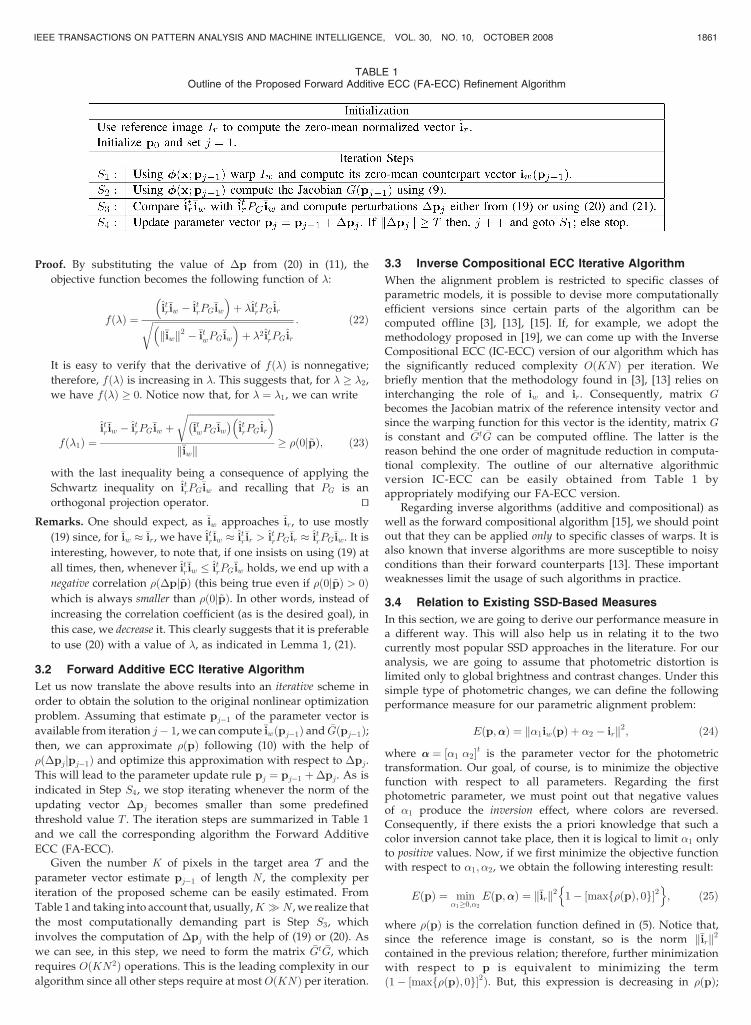
3.2 Forward Additive ECC Iterative Algorithm

Let us now translate the above results into an iterative scheme in

order to obtain the solution to the original nonlinear optimization

problem. Assuming that estimate pj�1 of the parameter vector is

available from iteration j� 1, we can compute�iwðpj�1Þ and �Gðpj�1Þ;then, we can approximate �ðpÞ following (10) with the help of

�ð�pjjpj�1Þ and optimize this approximation with respect to �pj.

This will lead to the parameter update rule pj ¼ pj�1 þ�pj. As is

indicated in Step S4, we stop iterating whenever the norm of the

updating vector �pj becomes smaller than some predefined

threshold value T . The iteration steps are summarized in Table 1

and we call the corresponding algorithm the Forward Additive

ECC (FA-ECC).Given the number K of pixels in the target area T and the

parameter vector estimate pj�1 of length N , the complexity per

iteration of the proposed scheme can be easily estimated. From

Table 1 and taking into account that, usually,K N , we realize that

the most computationally demanding part is Step S3, which

involves the computation of �pj with the help of (19) or (20). As

we can see, in this step, we need to form the matrix �Gt �G, which

requires OðKN2Þ operations. This is the leading complexity in our

algorithm since all other steps require at most OðKNÞ per iteration.

3.3 Inverse Compositional ECC Iterative Algorithm

When the alignment problem is restricted to specific classes ofparametric models, it is possible to devise more computationallyefficient versions since certain parts of the algorithm can becomputed offline [3], [13], [15]. If, for example, we adopt themethodology proposed in [19], we can come up with the InverseCompositional ECC (IC-ECC) version of our algorithm which hasthe significantly reduced complexity OðKNÞ per iteration. Webriefly mention that the methodology found in [3], [13] relies oninterchanging the role of iw and ir. Consequently, matrix G

becomes the Jacobian matrix of the reference intensity vector andsince the warping function for this vector is the identity, matrix Gis constant and �Gt �G can be computed offline. The latter is thereason behind the one order of magnitude reduction in computa-tional complexity. The outline of our alternative algorithmicversion IC-ECC can be easily obtained from Table 1 byappropriately modifying our FA-ECC version.

Regarding inverse algorithms (additive and compositional) aswell as the forward compositional algorithm [15], we should pointout that they can be applied only to specific classes of warps. It isalso known that inverse algorithms are more susceptible to noisyconditions than their forward counterparts [13]. These importantweaknesses limit the usage of such algorithms in practice.

3.4 Relation to Existing SSD-Based Measures

In this section, we are going to derive our performance measure ina different way. This will also help us in relating it to the twocurrently most popular SSD approaches in the literature. For ouranalysis, we are going to assume that photometric distortion islimited only to global brightness and contrast changes. Under thissimple type of photometric changes, we can define the followingperformance measure for our parametric alignment problem:

Eðp; ��Þ ¼ �1iwðpÞ þ �2 � irk k2; ð24Þ

where �� ¼ ½�1 �2�t is the parameter vector for the photometrictransformation. Our goal, of course, is to minimize the objectivefunction with respect to all parameters. Regarding the firstphotometric parameter, we must point out that negative valuesof �1 produce the inversion effect, where colors are reversed.Consequently, if there exists the a priori knowledge that such acolor inversion cannot take place, then it is logical to limit �1 onlyto positive values. Now, if we first minimize the objective functionwith respect to �1; �2, we obtain the following interesting result:

EðpÞ ¼ min�10;�2

Eðp; ��Þ ¼ k�irk2 1� max �ðpÞ; 0f g½ �2n o

; ð25Þ

where �ðpÞ is the correlation function defined in (5). Notice that,since the reference image is constant, so is the norm k�irk2

contained in the previous relation; therefore, further minimizationwith respect to p is equivalent to minimizing the termð1� ½maxf�ðpÞ; 0g�2Þ. But, this expression is decreasing in �ðpÞ;


TABLE 1Outline of the Proposed Forward Additive ECC (FA-ECC) Refinement Algorithm

consequently, we can equivalently maximize the correlationfunction �ðpÞ, thus recovering our criterion. The final optimizationproblem makes a lot of sense. Indeed, notice that, since �ðpÞ is freeof photometric distortions (the simple type we consider here) andunder the knowledge that there is no color inversion, it is quiteplausible to look for the most positive correlation.

If we drop the constraint �1 0, then the minimization of theobjective function in (25) is the optimization problem proposed byFuh and Maragos [6]. By optimizing first with respect to �1, �2

yields

EFMðpÞ ¼ min�1 ;�2

Eðp; ��Þ ¼ k�irk2 1� �2ðpÞ �

: ð26Þ

Notice that the resulting measure is now a decreasing function ofj�ðpÞj; therefore, any further minimization with respect to p isequivalent to maximizing the absolute value j�ðpÞj of thecorrelation function. It is clear that this optimization problemdoes not take into account the prior knowledge that there is nocolor inversion. In [6], maximization was achieved by adopting anexhaustive search approach in the N-D quantized parameterspace. Clearly, in a noncolor-inversion situation, such a search willgive rise to the correct maximum positive correlation (provided, ofcourse, that the warped image does not contain parts that are thenegative of the target area). However, as we mentioned inSection 1, exhaustive search approaches are characterized by highcomputational complexity, which becomes exceedingly demand-ing when we are interested in fine subpixel accuracy.

Although not proposed in [6], alternatively, we could adopt aniterative approach similar to the one suggested for our measure. If,however, we attempt to maximize j�ðpÞj using the same approx-imation as in (10), then one can show that the optimumperturbation �p is always given by (19). As was indicated inour remarks (after Lemma 1), adopting this strategy may result innegative correlations corresponding to local minima for �ðpÞinstead of the desired maxima. In other words, there are morechances for the iterative algorithm to be locked in erroneous localextrema than is the case with our approach.

An alternative measure arises if, in (24), we interchange theroles of iw and ir, that is,

Eðp; ��Þ ¼ �1ir þ �2 � iwðpÞk k2: ð27Þ

This is the approach adopted by Lucas and Kanade [10] and it isknown to generate, along with its variants, the most widely usedalgorithms in practice. Following similar steps as in the previoustwo cases, let us first minimize with respect to the two photometricparameters. This yields

ELKðpÞ ¼ min�1 ;�2

Eðp; ��Þ ¼ �iwðpÞ�� 2

1� �2ðpÞ �

: ð28Þ

We observe in the current outcome that the resulting criterion hastwo terms that depend on the parameters p, namely, the familiarpart f1� �2ðpÞg and the magnitude of the warped image k�iwðpÞk2

(which is not constant). Therefore, minimizing ELKðpÞwith respectto the parameters involves the minimization of the combination ofthe two terms. The first observation is that this criterion will notnecessarily produce the same solution as our measure. Second,due to the term k�iwðpÞk2, it is clear that an iterative algorithm canlock in solutions which result in k�iwðpÞk2 � 0 (for example, areaswith uniform intensity). And, third, because of the term �2ðpÞ, thealgorithm can lock in negative correlations.

Despite the previous observations, the Lucas-Kanade perfor-mance measure gives rise to the most popular iterative algo-rithms for the image alignment problem. For this reason, we aregoing to use it as a point of reference and compare it against ourscheme. Consequently, let us present its Forward Additive LK(FA-LK) updating version in more detail. Substituting the linear

approximation of �iwðpÞ in (28), then minimizing with respect to�p, we obtain the following optimum updating perturbation:

�pLK ¼ ð �Gt �GÞ�1 �Gt itr�iw � itrPG

�iw

1� itrPG irir ��iw

( ); ð29Þ

which is applicable at all times. Comparing (19) with (29), werealize that the difference is only in the scalar quantity thatprecedes the vector ir. As we are going to see, this seemingly slightvariation, in combination with (20), will result in significantperformance improvements.

For the Lucas-Kanade approach, it is possible to define a specialSSD-based measure that can handle arbitrary linear appearancevariations. For its minimization, an iterative algorithm that makesuse of the inverse additive update rule was proposed in [3] byHager and Belhumeur. Based on the same SSD measure, Bakeret al. [19], by adopting the inverse compositional approach,proposed several variants of the Hager-Belhumeur algorithm.Among these alternative algorithmic schemes, the SIC algorithm isreported to have the best performance [19]. Therefore, thisalgorithm will also be tested in the next section.

4 SIMULATION RESULTS

In this section, we perform a number of simulations in order toevaluate our FA-ECC and IC-ECC algorithmic version. As wementioned above, we will also simulate the FA-LK algorithmicversion that copes with photometric distortions and the SICalgorithm, which is considered to be the most effective inverseLK scheme. For all aspects affecting the simulation experiments,we made an effort to stay exactly within the framework specifiedin [13], [19]. To model the warping process, we are going to use theclass of affine transformations. We know that the 2D rigid body orsimilarity transformation are members of this class. Furthermore,the Jacobian of the affine model is a constant matrix, meaning thatit can be computed offline. Before proceeding with the presenta-tion of our simulation results, let us first briefly present theexperimental setup and the figures of merit we are going to adopt.

4.1 Experimental Setup and Figures of Merit

In order to create a reference and a warped image, we follow theprocedure proposed in [13]. In brief, let IðxÞ be a given image andxi, i ¼ 1; 2; 3, the coordinates of three points which define theboundaries of the desired target area. We perturb these points byadding Gaussian noise Nð0; �2

pÞ (�p captures the strength of thegeometric deformation), select a vector x0 such that the pointsx0 þ xi, i ¼ 1; 2; 3, lie in the interior of the support of the givenimage, and define the parameter vector pr of the affinetransformation that maps the original points to the translatednoisy ones. We apply this transformation to all points of the targetarea to warp it. With the help of bilinear interpolation, we computethe new intensities. This process defines the reference profile IrðxÞ.For the warped image, we use the given one.

All algorithms are initialized in the same way, namely,p0 ¼ ½1 0 0 1 xt0�

t. At iteration j, each algorithm provides theparameter estimates pj. In order to measure the quality of thisestimate, we use the following quantity:

eðjÞ ¼ 1

6

X3

i¼1

��ðxi; prÞ � ��ðxi; pjÞ�� 2

; ð30Þ

which quantifies the existing squared error between the exactwarped version of the points xi, i ¼ 1; 2; 3, and their estimatedcounterparts.

By averaging this error over many realizations that differ in thepoint noise realization, we can compute the Mean Square Distance


(MSD) value. Obviously, by computing this value in each iterationof an algorithm, we form a sequence that captures its learning

ability. Of course, it is unrealistic to expect that any of thealgorithms will converge at all times. This is particularly apparentfor high values of �p. For this reason, in order to quantify thealgorithmic performance in a meaningful way and have the rightpicture of this convergence characteristic, we adopt the ideafollowed in [13], namely, to define the MSD but conditioned on theevent that all of the competing algorithms have converged. By“convergence,” we mean that eðjmaxÞ � TMSD. In other words, weconsider that an algorithm has converged when its squared erroreðjÞ at a prescribed maximal iteration jmax is below a certainthreshold level TMSD.

The second quantity which is of importance is clearly thepercentage of converging (PoC) runs. Therefore, we define thisquantity as being the percentage of algorithms that converge up toa predefined maximal iteration jmax. PoC will be depicted as afunction of the point standard deviation �p, which is the mostimportant factor that affects the performance of all algorithms.

Since it is only natural to prefer an algorithm that convergesquickly with high probability, we propose a third figure of merit thatcaptures exactly this aspect. Specifically, for characteristic valuesof �p and thresholds TMSD, we apply the algorithms for a maximalnumber of iterations jMAX . Then, we compute the cumulative PoCachieved by each algorithm as jmax increases from 0 to jMAX . Thisthird figure of merit is proposed here for the first time.

In all of the experiments, we use the “Takeo” image as thewarped profile and generate a reference image as was previouslydescribed. We make 5,000 realizations of image pairs and we addindependent and identically distributed, zero-mean Gaussianintensity noise of standard deviation �i before running thecompeting algorithms. Although in [13], [19] we find threedifferent scenarios, here, due to lack of space, we only focus inthe one where we add noise to both image profiles (since this is themost interesting from a practical viewpoint).

4.2 First Experiment

In this experiment, for the intensity noise, we use a standarddeviation �i, which corresponds to eight gray levels, and comparethe convergency characteristics of the competing algorithms for amaximum number of iterations2 jmax ¼ 15 and TMSD ¼ 1 pixel2.Figs. 1a, 1b, and 1c depict the convergence profiles of thealgorithms for different values of �p. We observe the appearanceof an MSD floor value in each algorithm which is due to thepresence of the intensity noise. Fig. 1d presents the correspondingPoC as a function of �p.

As we can see, each algorithm attains a different MSD floorvalue with our FA-ECC version converging to the lowest one and

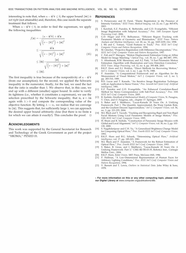
with a rate which can be significantly better. Specifically, for weakgeometric deformations, all algorithms reach almost comparablefloor values and have comparable convergence rates, with FA-ECCbeing slightly faster than its rivals. However, in the case ofmedium to strong deformations, FA-ECC reaches an MSD floorvalue which is 3 dB lower than the inverse versions and slightlylower than the FA-LK algorithm. On the other hand, theconvergency rate of FA-ECC is significantly superior comparedto all other algorithms. Regarding our IC-ECC version, as we cansee, it has performance comparable to the SIC algorithm. The samecharacteristics also apply to PoC, where FA-ECC exhibits a largerpercentage of successful convergences while IC-ECC matches theperformance of SIC. Regarding the third figure of merit, weapplied the algorithms for a maximal number of iterationsjMAX ¼ 100. In order to test the accuracy of the alignment, weselected a threshold value TMSD ¼ ð1=18 pixelÞ2 (i.e., �25 dB),assuring that TMSD is higher than the MSD floor value of allcompeting algorithms. Fig. 3a depicts the corresponding curves forthree values of �p. As we can see, for weak deformations, allalgorithms are almost completely successful after the10th iteration. When, however, the geometric deformation be-comes stronger, FA-ECC outperforms its competitors significantly.Again, IC-ECC is comparable to SIC.

4.3 Second Experiment

In this simulation, we consider the realistic case of photometricallydistorted images under noisy conditions. We consider twodifferent scenarios. We impose the photometric distortion 1) onthe reference image and 2) on the warped one. Since all competingalgorithms perfectly compensate for linear photometric distor-tions, we consider a nonlinear transformation of the formIðxÞ ðIðxÞ þ 20Þ0:9, which is applied to the intensity of eachimage pixel. We repeat the same set of simulations as in the firstexperiment, only now we impose the photometric distortion beforeadding intensity noise.

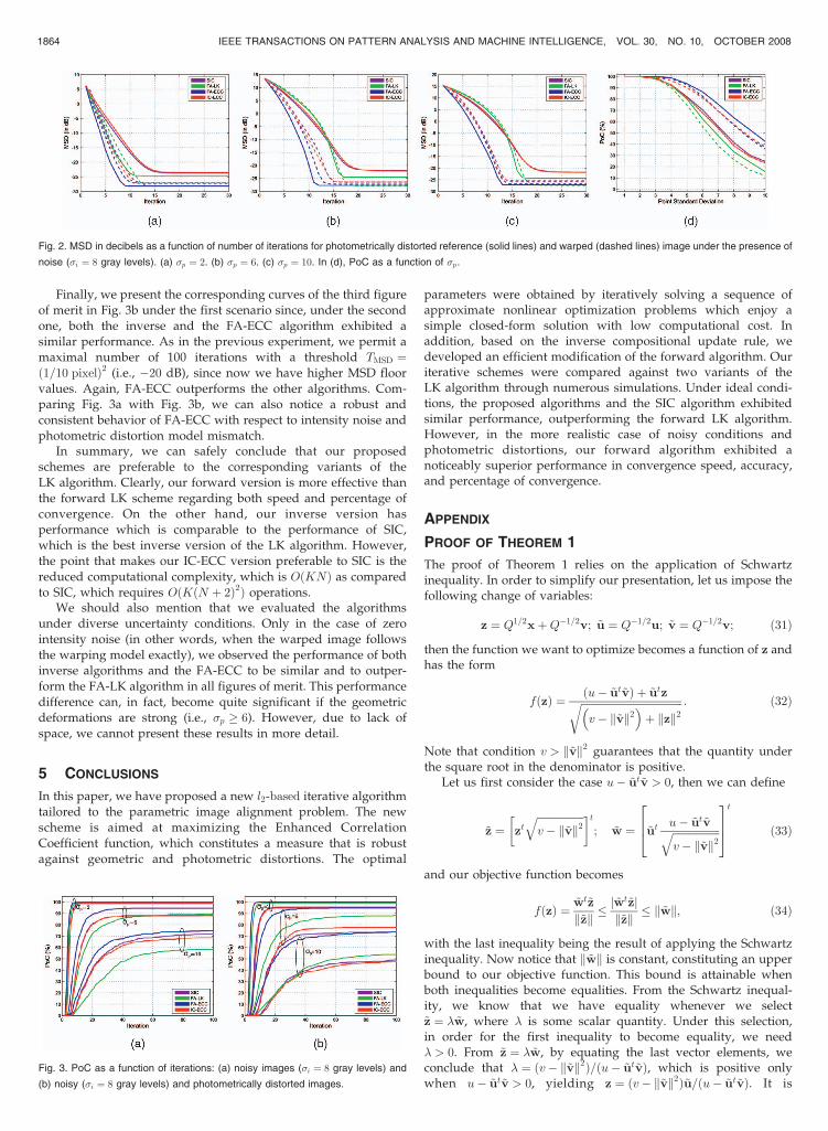
The results we obtained are shown in Fig. 2. As we can see, theperformance of our forward algorithm seems to be almostunaffected, achieving, under both scenarios, almost the same andthe lowest MSD floor value. On the other hand, the performance ofboth inverse algorithms and FA-LK scheme seems to be vitallyaffected. Comparing Fig. 2 with Fig. 1, we observe that, under thefirst scenario, FA-ECC performs even better than before. In fact,the MSD floor value is now 3 and 5 dB lower than the valueattained by the FA-LK algorithm and the inverse algorithms,respectively. We should note here that the MSD floor is due notonly to the intensity noise but also to the photometric modelmismatch. Under the second scenario, all algorithms achieve thesame MSD floor value. As far as PoC is concerned, we observe arather steady and robust behavior for the forward algorithmsunder both scenarios while inverse schemes, under the firstscenario, exhibit a significant performance reduction as comparedto the second one.


2. In order to make the different MSD floor values achieved by thecompeting algorithms in Figs. 1a, 1b, and 1c and Figs. 2a, 2b, and 2c visible,30 iterations are shown.

Fig. 1. MSD in decibels as a function of number of iterations under the presence of noise (�i ¼ 8 gray levels). (a) �p ¼ 2. (b) �p ¼ 6. (c) �p ¼ 10. In (d), PoC as a function

of �p.

Finally, we present the corresponding curves of the third figureof merit in Fig. 3b under the first scenario since, under the secondone, both the inverse and the FA-ECC algorithm exhibited asimilar performance. As in the previous experiment, we permit amaximal number of 100 iterations with a threshold TMSD ¼ð1=10 pixelÞ2 (i.e., �20 dB), since now we have higher MSD floorvalues. Again, FA-ECC outperforms the other algorithms. Com-paring Fig. 3a with Fig. 3b, we can also notice a robust andconsistent behavior of FA-ECC with respect to intensity noise andphotometric distortion model mismatch.

In summary, we can safely conclude that our proposedschemes are preferable to the corresponding variants of theLK algorithm. Clearly, our forward version is more effective thanthe forward LK scheme regarding both speed and percentage ofconvergence. On the other hand, our inverse version hasperformance which is comparable to the performance of SIC,which is the best inverse version of the LK algorithm. However,the point that makes our IC-ECC version preferable to SIC is thereduced computational complexity, which is OðKNÞ as comparedto SIC, which requires OðKðN þ 2Þ2Þ operations.

We should also mention that we evaluated the algorithmsunder diverse uncertainty conditions. Only in the case of zerointensity noise (in other words, when the warped image followsthe warping model exactly), we observed the performance of bothinverse algorithms and the FA-ECC to be similar and to outper-form the FA-LK algorithm in all figures of merit. This performancedifference can, in fact, become quite significant if the geometricdeformations are strong (i.e., �p 6). However, due to lack ofspace, we cannot present these results in more detail.

5 CONCLUSIONS

In this paper, we have proposed a new l2-based iterative algorithmtailored to the parametric image alignment problem. The newscheme is aimed at maximizing the Enhanced CorrelationCoefficient function, which constitutes a measure that is robustagainst geometric and photometric distortions. The optimal

parameters were obtained by iteratively solving a sequence ofapproximate nonlinear optimization problems which enjoy asimple closed-form solution with low computational cost. Inaddition, based on the inverse compositional update rule, wedeveloped an efficient modification of the forward algorithm. Ouriterative schemes were compared against two variants of theLK algorithm through numerous simulations. Under ideal condi-tions, the proposed algorithms and the SIC algorithm exhibitedsimilar performance, outperforming the forward LK algorithm.However, in the more realistic case of noisy conditions andphotometric distortions, our forward algorithm exhibited anoticeably superior performance in convergence speed, accuracy,and percentage of convergence.

APPENDIX

PROOF OF THEOREM 1

The proof of Theorem 1 relies on the application of Schwartzinequality. In order to simplify our presentation, let us impose thefollowing change of variables:

z ¼ Q1=2xþQ�1=2v; ~u ¼ Q�1=2u; ~v ¼ Q�1=2v; ð31Þ

then the function we want to optimize becomes a function of z andhas the form

fðzÞ ¼ ðu� ~ut~vÞ þ ~utzffiffiffiffiffiffiffiffiffiffiffiffiffiffiffiffiffiffiffiffiffiffiffiffiffiffiffiffiffiffiffiffiffiffiffiffiffiffiffiv� k~vk2

þ kzk2

r : ð32Þ

Note that condition v > k~vk2 guarantees that the quantity underthe square root in the denominator is positive.

Let us first consider the case u� ~ut~v > 0, then we can define

~z ¼ ztffiffiffiffiffiffiffiffiffiffiffiffiffiffiffiffiffiffiv� k~vk2

q� �t; ~w ¼ ~ut

u� ~ut~vffiffiffiffiffiffiffiffiffiffiffiffiffiffiffiffiffiffiv� k~vk2

q264

375t

ð33Þ

and our objective function becomes

fðzÞ ¼ ~wt~z

k~zk �j ~wt~zjk~zk � k ~wk; ð34Þ

with the last inequality being the result of applying the Schwartzinequality. Now notice that k ~wk is constant, constituting an upperbound to our objective function. This bound is attainable whenboth inequalities become equalities. From the Schwartz inequal-ity, we know that we have equality whenever we select~z ¼ � ~w, where � is some scalar quantity. Under this selection,in order for the first inequality to become equality, we need� > 0. From ~z ¼ � ~w, by equating the last vector elements, weconclude that � ¼ ðv� k~vk2Þ=ðu� ~ut~vÞ, which is positive onlywhen u� ~ut~v > 0, yielding z ¼ ðv� k~vk2Þ~u=ðu� ~ut~vÞ. It is


Fig. 2. MSD in decibels as a function of number of iterations for photometrically distorted reference (solid lines) and warped (dashed lines) image under the presence of

noise (�i ¼ 8 gray levels). (a) �p ¼ 2. (b) �p ¼ 6. (c) �p ¼ 10. In (d), PoC as a function of �p.

Fig. 3. PoC as a function of iterations: (a) noisy images (�i ¼ 8 gray levels) and

(b) noisy (�i ¼ 8 gray levels) and photometrically distorted images.

interesting to note that, when u� ~ut~v � 0, the upper bound k ~wk isnot tight (not attainable) and, therefore, this case needs the separatetreatment that follows.

When u� ~ut~v � 0, in order to find the supremum, we applythe following inequalities:

fðzÞ ¼ ðu� ~ut~vÞ þ ~utzffiffiffiffiffiffiffiffiffiffiffiffiffiffiffiffiffiffiffiffiffiffiffiffiffiffiffiffiffiffiffiffiffiffiffiffiffiffiffiv� k~vk2

þ kzk2

r

� ~utzffiffiffiffiffiffiffiffiffiffiffiffiffiffiffiffiffiffiffiffiffiffiffiffiffiffiffiffiffiffiffiffiffiffiffiffiffiffiffiv� k~vk2

þ kzk2

r

� k~uk kzkffiffiffiffiffiffiffiffiffiffiffiffiffiffiffiffiffiffiffiffiffiffiffiffiffiffiffiffiffiffiffiffiffiffiffiffiffiffiffiv� k~vk2

þ kzk2

r� k~uk:

ð35Þ

The first inequality is true because of the nonpositivity of u� ~ut~v(from our assumption); for the second, we applied the Schwartzinequality in the numerator; finally, for the last, we used the factthat the ratio is smaller than 1. We observe that, in this case, weend up with a different (smaller) upper bound. In order to verifyits tightness (i.e., whether it constitutes a supremum), we use theselection prescribed by the Schwartz inequality, that is, z ¼ �~uagain with � > 0 and compute the corresponding value of theobjective function. By letting �!1, we realize that we convergeto k~uk. This suggests that, for sufficiently large �, we can approachthe desired upper bound arbitrarily close (but there is no finite zfor which we can attain it exactly!). This concludes the proof. tu

ACKNOWLEDGMENTS

This work was supported by the General Secretariat for Researchand Technology of the Greek Government as part of the project“XROMA,” PENED 01.

REFERENCES

[1] S. Periaswamy and H. Farid, “Elastic Registration in the Presence ofIntensity Variation,” IEEE Trans. Medical Imaging, vol. 22, no. 7, pp. 865-874,2003.

[2] I. Karybali, E.Z. Psarakis, K. Berberidis, and G.D. Evangelidis, “EfficientImage Registration with Subpixel Accuracy,” Proc. 14th European SignalProcessing Conf., 2006.

[3] G.D. Hager and P.N. Belhumeur, “Efficient Region Tracking withParametric Models of Geometry and Illumination,” IEEE Trans. PatternAnalysis and Machine Intelligence, vol. 20, no. 10, pp. 1025-1039, Oct. 1998.

[4] J. Shi and C. Tomasi, “Good Features to Track,” Proc. IEEE Int’l Conf.Computer Vision and Pattern Recognition, 1994.

[5] M. Gleicher, “Projective Registration with Difference Decomposition,” Proc.IEEE Int’l Conf. Computer Vision and Pattern Recognition, 1997.

[6] C. Fuh and P. Maragos, “Motion Displacement Estimation Using an AffineModel for Image Matching,” Optical Eng., vol. 30, no. 7, pp. 881-887, 1991.

[7] Y. Altunbasak, R.M. Mersereau, and A.J. Patti, “A Fast Parametric MotionEstimation Algorithm with Illumination and Lens Distortion Correction,”IEEE Trans. Image Processing, vol. 12, no. 4, pp. 395-408, 2003.

[8] B.K.P. Horn and E.J. Weldon, “Direct Methods for Recovering Motion,”Int’l J. Computer Vision, vol. 2, no. 1, pp. 51-76, 1988.

[9] P. Anandan, “A Computational Framework and an Algorithm for theMeasurement of Visual Motion,” Int’l J. Computer Vision, vol. 2, no. 3,pp. 283-310, 1989.

[10] B.D. Lucas and T. Kanade, “An Iterative Image Registration Techniquewith an Application to Stereo Vision,” Proc. Seventh Int’l Joint Conf. ArtificialIntelligence, 1981.

[11] E.Z. Psarakis and G.D. Evangelidis, “An Enhanced Correlation-BasedMethod for Stereo Correspondence with Sub-Pixel Accuracy,” Proc. 10thIEEE Int’l Conf. Computer Vision, 2005.

[12] R. Szeliski, Handbook of Mathematical Models of Computer Vision, N. Paragios,Y. Chen, and O. Faugeras, eds., chapter 17. Springer, 2005.

[13] S. Baker and I. Matthews, “Lucas-Kanade 20 Years On: A UnifyingFramework: Part 1. The Quantity Approximated, the Warp Update Rule,and the Gradient Descent Approximation,” Int’l J. Computer Vision, vol. 56,no. 3, pp. 221-255, 2004.

[14] M.J. Black and Y. Yacoob, “Tracking and Recognizing Rigid and Non-RigidFacial Motions Using Local Parametric Models of Image Motion,” Proc.Fifth IEEE Int’l Conf. Computer Vision, 1995.

[15] H. Shum and R. Szeliski, “Construction of Panoramic Image Mosaics withGlobal and Local Alignment,” Int’l J. Computer Vision, vol. 36, no. 2, pp. 101-130, 2000.

[16] S. Nagahdaripour and C.H. Yu, “A Generalized Brightness Change Modelfor Computing Optical Flow,” Proc. Fourth IEEE Int’l Conf. Computer Vision,1993.

[17] B.K.P. Horn and B.G. Schunk, “Determining Optical Flow,” ArtificialIntelligence, vol. 17, pp. 185-203, 1981.

[18] M.J. Black and P. Anandan, “A Framework for the Robust Estimation ofOptical Flow,” Proc. Fourth IEEE Int’l Conf. Computer Vision, 1993.

[19] S. Baker, R. Gross, and I. Matthews, “Lucas-Kanade 20 Years On: AUnifying Framework: Part 3,” CMU-RI-TR-03-35, Robotics Inst., CarnegieMellon Univ., 2004.

[20] B.K.P. Horn, Robot Vision. MIT Press, McGraw-Hill, 1986.[21] P. Hallinan, “A Low-Dimensional Representation of Human Faces for

Arbitrary Lighting Conditions,” Proc. IEEE Int’l Conf. Computer Vision andPattern Recognition, 1994.

[22] V. Barnett and T. Lewis, Outliers in Statistical Data. John Wiley & Sons,1978.

. For more information on this or any other computing topic, please visitour Digital Library at www.computer.org/publications/dlib.


parametric image alignment using enhanced correlation coefficient maximization

Documents