Journal of Hydrology 380 (2010) 82–93

Contents lists available at ScienceDirect

Journal of Hydrology

journal homepage: www.elsevier .com/locate / jhydrol

Parameter optimization and uncertainty analysis for plot-scale continuousmodeling of runoff using a formal Bayesian approach

E. Laloy *, D. Fasbender, C.L. BieldersDepartment of Environmental Sciences and Land Use Planning, Université catholique de Louvain (UCL), Croix du Sud, 2 Bte 2, B-1348 Louvain-la-Neuve, Belgium

a r t i c l e i n f o s u m m a r y

Article history:Received 26 June 2009Received in revised form 23 October 2009Accepted 25 October 2009

This manuscript was handled byA. Bardossy, Editor-in-Chief, with theassistance of John W. Nicklow,Associate Editor

Keywords:Continuous runoff modelParameter optimizationParameter uncertaintyMarkov Chain Monte CarloDREAMResiduals autocorrelation

0022-1694/$ - see front matter � 2009 Elsevier B.V. Adoi:10.1016/j.jhydrol.2009.10.025

* Corresponding author. Tel.: +32 10 47 37 27; fax:E-mail address: eric.laloy@uclouvain.be (E. Laloy).

This study reports on the use the recently developed Differential Evolution Adaptative Metropolis algo-rithm (DREAM) to calibrate in a Bayesian framework the continuous, spatially distributed, process-basedand plot-scale runoff model described by Laloy and Bielders (2008). The calibration procedure, relying on2 years of daily runoff measurements, accounted for heteroscedasticity and autocorrelation. This resultedin a realistic estimation of parameter uncertainty and its impact on model predictions. The calibratedmodel reproduced the observed hydrograph satisfactorily during calibration. The model validation onan independent 1-year series of measurements showed reasonable values for the Nash–Sutcliffe effi-ciency criterion. This was equal to 0.76 and 0.78 for, respectively, the upper and lower bounds of the95% uncertainty interval associated with parameter uncertainty. However, the fact that this intervalwas always very narrow but often did not bracket the observations during the validation period indicatesthat, assuming observational errors to be negligible, model structure has to be improved in order toachieve more accurate predictions. Overall the methodology allowed to efficiently discriminate betweenparameter and total predictive uncertainty and to highlight scope for model improvement.

� 2009 Elsevier B.V. All rights reserved.

Introduction

The parameterization of rainfall–runoff models is an importantbut difficult task because many of the parameters in these modelsare not directly measurable in the field and therefore can only beobtained through calibration against a historical record of data.Model calibration consists of tuning the values of unknown or par-tially known model parameters, such that the model predictions fitas closely and consistently as possible to the observations. This canbe done by visual adjustment but the subjective and time-consum-ing nature of the trial-and-error method makes this approach dif-ficult for models with a large number of parameters. In this widelyencountered case, an automatic calibration procedure is necessary.

Automatic parameter optimization techniques have been widelyused in the area of surface water hydrology for several decades(Sorooshian and Dracup, 1980; Kuczera, 1983; Duan et al., 1992;Vrugt et al., 2003; Cooper et al., 2007; Feyen et al., 2007; Vrugtand Robinson, 2007). The main difficulties preventing the determi-nation of the best parameter set by any automatic calibration algo-rithm are the presence of multiple local optima, nonlinearinteraction between model parameters and the complex shape of

ll rights reserved.

+32 10 47 38 33.

the response surface defined by the objective function (Feyenet al., 2007). To overcome these problems, global optimization tech-niques were developed such as the Shuffled Complex Evolutionmethod (Duan et al., 1992) or simulated annealing (Sumner et al.,1997). These methods seek to determine unique global solutionsbut do not provide any information regarding the confidence thatcan be attributed to the parameter estimates. However, since pro-cess-based hydrological models consist, at least partially, of anempirical combination of mathematical relationships describingsome observable features of idealized hydrological processes (Kucz-era and Parent, 1998), parameter estimates are subject to uncer-tainty, which leads to uncertainty in model predictions. In manyapplications this uncertainty needs to be quantified to providemeaningful model results. In the area of surface water hydrology,the parameter uncertainty must be assessed in order to regionalizeor relate model parameters to measurable soil or catchment charac-teristics or to evaluate confidence limits on model response.

Many approaches have been developed to assess parameteruncertainty and its effects on model predictions. These includethe use of multinormal approximations (Kuczera and Mroczkow-ski, 1998), multimodel ensembles (Georgakakos et al., 2004) andMonte Carlo-based methods like uniform sampling over an hyper-cube (Beven and Binley, 1992; Uhlenbrook et al., 1999; Iorgulescuet al., 2005) and Markov Chain Monte Carlo (MCMC) methods

E. Laloy et al. / Journal of Hydrology 380 (2010) 82–93 83

(Kuczera and Parent, 1998; Vrugt et al., 2003), just to name a few.As opposed to Monte Carlo methods, approaches based on first-or-der approximations and multinormal distributions are typicallyunable to cope with the nonlinearity of complex hydrological mod-els (Kuczera and Parent, 1998; Vrugt and Boutem, 2002; Gallagherand Doherty, 2007). On the other hand, uniform Monte Carlo sam-pling is computationally inefficient and cannot maintain an ade-quate sampling density as the number of parameters increases,which is likely to lead to unreliable results. For continuous mul-ti-variable problems, the MCMC sampler approach is therefore anattractive method to assess model parameter uncertainty.

The aim of the present paper is to assess, within a formal Bayes-ian framework, the parameter uncertainty and its effects on modelpredictions, for the continuous, plot-scale, rainfall–runoff model ofLaloy and Bielders (2008). This model constitutes the hydrologicalcomponent of the CREHDYS erosion model Laloy and Bielders(2009a,b). This is done using a new Monte Carlo Markov Chainsampler called the Differential Evolution Adaptative Metropolisalgorithm (DREAM), recently developed by Vrugt et al. (2009a).The DREAM scheme is a follow-up of the Shuffled Complex Evolu-tion Metropolis global optimization method (SCEM-UA: Vrugtet al., 2003) that has the advantage of maintaining detailed balanceand ergodicity while showing good efficiency for complex, highlynonlinear and multimodal target distributions (Vrugt et al.,2009a). Runoff data from a 3-year continuous maize croppingsystem was selected as a case study.

Methodology

Parameter estimation within the Bayesian framework

The n sized vector of simulated outputs Y ¼ fy1; . . . ; yng of anyrainfall–runoff model / can be written as:

Y ¼ /ðb; xÞ ð1Þ

where b is the vector of model parameters and x represents themeasured input values, i.e. boundary (forcing) conditions and initialconditions. A very common way to assess the model’s ability to sim-ulate the underlying system is to compare the vector of model out-puts Y with a vector of n observed data bY ¼ fy1; . . . ; yng bycomputing:

eiðb; bY; xÞ ¼ yiðb; xÞ � yi ð2Þ

where the ei are the elements of e, the vector of residuals. The closerto zero are the residuals, the better the model simulates the ob-served data. Classically in rainfall–runoff model parameter single-objective estimation, the parameter vector b that results in the bestmodel behavior is found by tuning the values in b so as to minimizethe Sum of Squared Residuals (SSR):

SSRðb; bY; xÞ ¼Xn

i¼1

eiðb; bY; xÞ2h ið3Þ

However, estimates of hydrological model parameters are nevererror-free, because the calibration data contain measurement er-rors, different parameter combinations may have similar influenceon model output and the model never perfectly simulates the sys-tem. Consequently, it is often impossible to derive a unique bestparameter set and the parameter uncertainty resulting from thecalibration process must be assessed if we want to evaluate confi-dence limits on model response. It is therefore desirable to esti-mate not only the optimal values of the parameter set b but alsothe probability density function (pdf) of b; pðbjbY; xÞ. The pdf of brepresents the probabilistic information about the parameter setb given the measurements bY, the initial and forcing conditions x

and any a priori knowledge about b. Bayesian statistics coupledwith Monte Carlo sampling is one possible approach to estimatepðbjbY; xÞ.

According to the Bayes theorem, the posterior pdf pðbjbY; xÞ isproportional to the product of the likelihood function and the priorpdf. The prior pdf with probability density function pðbÞ summa-rizes the a priori knowledge about b. It often consists in realisticlower and upper bounds on each of the parameters, which definethe expected parameter space, and imposing a uniform prior distri-bution on this hyper rectangle (Vrugt et al., 2003). Assuming thatmeasurement errors in Eq. (2) are normally distributed, homosce-dastic and uncorrelated in time, the likelihood function of param-eter set b is given by (Box and Tiao, 1973):

Lðb;re; bY; xÞ / exp �12

Xn

i¼1

eiðb; bY; xÞre

" #20@ 1A ð4Þ

where r2e is the measurement error variance. In hydrological mod-

eling, re is usually unknown and, when needed, estimated a poste-riori from the quality of the fit by computing the root mean squareerror associated with the considered model run. This implicitly as-sumes a zero model error (see Vrugt and Boutem (2002) for anextensive discussion).

To handle a violation of the homoscedasticity assumption, aBox–Cox transformation (Box and Cox, 1964) with parameter kcan be applied to measured bY and simulated Y data:

bY� ¼ ðbYk � 1Þ=k if k – 0

lnðbYÞ if k ¼ 0

(ð5Þ

and

Y� ¼ ðYk � 1Þ=k if k – 0lnðYÞ if k ¼ 0

(ð6Þ

The elements e�i of the vector of transformed residuals e� aretherefore given by:

e�i ðb; k; bY�; xÞ ¼ y�i ðb; k; xÞ � y�i ð7Þ

One must note that this way of handling heteroscedasticityimplicitly assumes that the posterior parameter pdf obtained inthe transformed output space also holds for the untransformedoutput space despite the nonlinearity in the Box–Coxtransformation.

Residuals of rainfall–runoff models are often autocorrelatedbecause of uncertainties inherent in the observed data and struc-tural inadequacies in the mathematical model representation ofthe hydrological processes (Sorooshian and Dracup, 1980; Feyenet al., 2007; Schaefli et al., 2007) as well as of natural process auto-correlation. To account, at least partially, for time dependence ofthe residuals, a first-order autoregressive time series model (AR1)can be applied to the residuals. AR1 models are the most widelyused type of autoregressive moving average time series model(ARMA, see Box and Jenkins (1976), for details) in the hydrologicalliterature to account for time correlated error (Sorooshian and Dra-cup, 1980; Kuczera, 1983; Yang et al., 2007; Schaefli et al., 2007;Vrugt et al., 2009b). The general AR1 scheme of the transformedresiduals is given by:

e�i ¼ qe�i�1 þ di i ¼ 1; . . . ;n ð8Þ

where q is a first-order autoregressive parameter, i is the position ofthe considered residual in the transformed residuals vector of sizen; e�0 ¼ 0 and d � N 0;r2

d

� �is the remaining (unexplained) error

with zero mean and constant variance r2d . Correcting the time series

of the transformed residuals e� by the AR1 scheme gives then(Sorooshian and Dracup, 1980):

84 E. Laloy et al. / Journal of Hydrology 380 (2010) 82–93

diðb; k;q; bY�; xÞ ¼ e�i ðb; k; bY�; xÞ � qe�i�1ðb; k; bY�; xÞ i ¼ 1; . . . ;n

ð9Þ

In order to allow interaction between the model parametersand the AR1 corrected transformed residuals, the k parameterand q coefficient can be added to the optimization problem. Doingso, incorporating the AR1 model into the likelihood function ofb; k; q; Y�; x and r2

d (see Sorooshian and Dracup (1980), for a de-tailed derivation of the right hand side term) gives:

L b; k;q;rd; bY�; x;� �/ exp �1

2e�1ðb; k; bY�; xÞ2ð1� q2Þ þ

Pni¼2diðb; k;q; bY�; xÞ2

r2d

" # !ð10Þ

Note that for q ¼ 0 and untransformed residuals (no Box–Coxtransformation), Eq. (10) reduces to Eq. (4). Assuming that b, k; qand r2

d are independent, the joint posterior pdf of b, k, q and rd

is then given by:

pðb; k;q;rdjbY�; xÞ / Lðb; k;q;rd; bY�; xÞpðbÞpðkÞpðqÞpðrdÞ ð11Þ

where pðkÞ; pðqÞ and pðrdÞ are the prior pdfs of k; q and rd, respec-tively. Assuming a non-informative prior pdf of the form pðrdÞ /r�1

d for rd and uniform prior pdfs for b; k and q, the joint posteriorpdf of b; k; q and rd may therefore be written as:

pðb;k;q;rdjbY�;x;Þ/exp �1

2

e�1 b;k; bY�;x� �2ð1�q2Þþ

Pni¼2diðb;k;q;bY�;xÞ2

r2d

264375

0B@1CApðrdÞ

ð12Þ

Finally, the influence of rd can be integrated out leading to thejoint posterior pdf of vector b; k parameter and q coefficient:

pðb; k;qjbY; xÞ ¼ Z p b; k;q;rdjbY; x� �drd ð13aÞ

pðb; k;qjbY; xÞ ¼ C�1 e�1 b; k; bY�; x� �2ð1� q2Þ

�

þXn

i¼2

diðb; k;q; bY�; xÞ2#�n

2

ð13bÞ

where C ¼R

e�1ðb; k; bY�; xÞ2ð1� q2Þ þPn

i¼2diðb; k;q; bY�; xÞ2h i�n2dbdk

dq is the normalising constant. Note that Eq. (13b) explicitly treatsthe effect of model structural error through autocorrelation of theresiduals, but does not account for potential errors in initial andforcing conditions. Consequently, x is an approximation of x.

Rainfall forcing errors typically dominate other input errors atthe catchment scale because of the significant spatial and temporalvariability of rainfall fields. However, given that our field context isa plot-scale situation (see section ‘‘Case study”) where the plots arerelatively small ð90 m2Þ and the rainfall measurement device (acalibrated tipping bucket rain gauge) is located in the very closevicinity of the plots, the rainfall forcing uncertainty was consideredas negligible. Furthermore, the mechanical error associated withtipping bucket rain gauges does not exceed 5% for rainfall intensi-ties lower than 200 mm h�1 (Fankhauser, 1997; Molini et al., 2005;Stransky et al., 2007).

In addition, the uncertainty on the measured 1-min runoff rateaggregated into daily volumes (see explanation in section ‘‘Thehydrological model”) was also considered negligible, given thatthe outflow measurement device was experimentally precisely cal-ibrated with a small error. This led to a constrained eight-variable

optimization problem for which the posterior parameter pdf is gi-ven by Eq. (13b).

Sampling a posterior distribution using the DREAM algorithm

The Monte Carlo Markov Chain (MCMC) schemes constitute ageneral approach for sampling from a posterior probability densityfunction pðbY�; xÞ. The main feature behind this approach is to builda Markov Chain that generates a random walk through the param-eter space with stable frequency stemming from a fixed probabilitydistribution (Vrugt et al., 2003). A Markov Chain is generated bysampling bðtþ1Þ � zðbjbðtÞÞ; t being the iteration number. The zfunction, called the proposal distribution of the Markov Chain, gen-erates bðtþ1Þ only from bðtÞ and not from bð0Þ;bð1Þ; . . . ;bðt�1Þ. The ear-liest and most general MCMC method is the random walkMetropolis–Hastings (RWMH) algorithm (Metropolis et al., 1953;Hastings, 1970) which is fully described in e.g., Gelman et al.(1995), Vrugt et al. (2003) and Schaefli et al. (2007). It has beenproven that this algorithm will generate a sequence of parametersets that converges to the posterior pdf pðbjbY�; xÞ for sufficientlylarge t (Gelman et al., 1995). However, this convergence dependson the shape and the size of the proposal distribution z().

In practice, an inappropriate z will lead to an impractically slowconvergence rate (Vrugt et al., 2009a). Ways to increase the searchefficiency of MCMC methods are to run several chains in parallelwith different starting points to best explore the parameter spaceas well as to continuously update the proposal distribution z() ineach chain, using information from past states. Theses ideas haveled to the development of the Shuffled Complex Evolution Metrop-olis method (SCEM-UA: see Vrugt et al., 2003). However, there isno formal proof of convergence of the procedure used in SCEM-UA for updating the proposal distribution. Moreover, the use of acovariance matrix in the proposal distribution (see Vrugt et al.,2003) may make it difficult to sample a multimodal distributionwith disconnected modes. These reasons have recently led to thedevelopment of the DiffeRential Evolution Adaptative Metropolisalgorithm (DREAM: Vrugt et al., 2009a) for which convergenceproperties are proven and which is used in this study.

The algorithm is detailed in Vrugt et al. (2009a,c). Therefore,this paper provides only a brief description regarding the way inwhich the convergence of the algorithm is controlled. When a pre-specified number of draws is reached, the search convergence to astable distribution is monitored with the R criterion of Gelman andRubin (1992) based on the within and between chain variance ofeach parameter (see also Vrugt and Boutem, 2002). This criterionmust be calculated by merging the chain elements generated aftera so-called burn-in period necessary for the algorithm to becomeindependent of its initial values. An R factor value of less than1.2 for each parameter is required to declare convergence to a sta-tionary distribution.

Quantifying the effect of parameter and total errors on modelpredictions

To understand how the uncertainty in model parameters trans-lates into predictive uncertainty, 95% prediction uncertaintybounds associated with parameter uncertainty were constructedby sampling i ¼ 1; . . . ;2500 posterior combinations of all the opti-mization variables (model parameters bi, Box–Cox coefficient ki

and first-order autoregressive coefficient qi) and running the mod-el to obtain an ensemble of 2500 different hydrographs Yi. Then, a95% confidence interval on model prediction was built by calculat-ing the 2.5% and 97.5% percentiles, respectively.

However, besides the effect of parameter uncertainty, a notexplicitly assessed error term � is likely to remain associated witheach model prediction generated from the posterior pdf of model

E. Laloy et al. / Journal of Hydrology 380 (2010) 82–93 85

parameters. A 95% total predictive uncertainty interval shouldintegrate this remaining unexplained error that is presumablydue to model structural inadequacies that are not covered by theinferred AR1 model and, to a much lesser extent in the presentcase, to untreated observational errors. Assuming � to be additive,Vrugt et al. (2009b) proposed the following equation to determine�i associated with each model prediction ðY�Þi in the transformedoutput space:

�i � N 0; r2d

� �i

�½1� ðq2Þi�

� �ð14Þ

Following Sorooshian and Dracup (1980), r2d may be approxi-

mated by the mean square error of the transformed, AR1 correctederror model:

r2d ¼

1n

e�1� �2ð1� q2Þ þ

Xn

j¼2

d2j

" #ð15Þ

whereas Vrugt et al. (2009b) computed r2d by multiplying the out-

come of Eq. (15) by n=z where z is drawn from a chi-squared distri-bution with n degrees of freedom. This approach is slightly moreefficient. Indeed, if the d residuals follow a zero-mean Gaussian dis-tribution with constant variance r2

d , then their sum of squares di-vided by r2

d follows a chi-squared distribution with n degrees offreedom.

Doing so allows to compute ðZ�Þi ¼ ðY�Þi þ �i for each draw i

sampled from the posterior pdf of b; k and q. After back-trans-forming the i ¼ 1; . . . ;2500 ðZ�Þi output time series to the originaloutput space (leading to i ¼ 1; . . . ;2500 ðZÞi vectors), a 95% totalpredictive uncertainty interval can again be constructed by calcu-lating the 2.5% and 97.5% percentiles.

The hydrological model

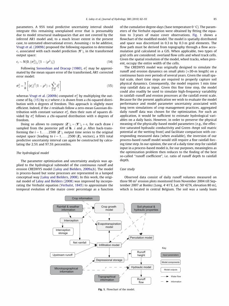
The parameter optimization and uncertainty analysis was ap-plied to the hydrological submodel of the continuous runoff anderosion CREDHYS model (Laloy and Bielders, 2009a,b). The modelis process-based but some processes are represented in a lumpedconceptual way (Laloy and Bielders, 2008). In this work, the origi-nal model of Laloy and Bielders (2008) was improved by incorpo-rating the Verhulst equation (Verhulst, 1845) to approximate thetemporal evolution of the maize cover percentage as a function

Fig. 1. Flowchart

of the cumulative degree-days (base temperature 0 �C). The param-eters of the Verhulst equation were obtained by fitting the equa-tion to 3 years of maize cover observations. Fig. 1 shows aflowchart of the modified model. The model is spatially distributedand space was discretized in 0.3 m by 0.3 m grid elements. Theflow path must be derived from topography through a flow accu-mulation grid calculated in a GIS. When applicable, two types ofgrid cells are considered: overland flow cells and wheel track cells.Given the spatial resolution of the model, wheel tracks, when pres-ent, occupy the entire width of the cells.

The CREDHYS model was originally designed to simulate therunoff and erosion dynamics on small plots (�30-m length) on acontinuous basis over periods of several years. Given the small spa-tial scale, short time steps are required to properly capture soilphysical dynamics. Consequently, the model requires 1 min timestep rainfall data as input. Given this fine time step, the modelcould also readily be used to simulate high-frequency variabilityin rainfall–runoff and erosion processes at the rainfall event scale.Because for the present application we wish to evaluate the modelperformance and model parameter uncertainty associated withlong term simulations of crop management practices, aggregateddaily runoff data was chosen for the optimization. For such anapplication, it would be sufficient to estimate hydrological vari-ables on a daily basis. However, in order to preserve the physicalmeaning of the physically-based model parameters (e.g., the effec-tive saturated hydraulic conductivity and Green–Ampt soil matricpotential at the wetting front) and facilitate comparison with cor-responding measured data (when available), the inversion of ourprocess-based runoff model would still require a fine rainfall forc-ing time step. In our opinion, the use of a daily time step for rainfallinput in a process-based model is, for our purposes, meaningless asthe optimization problem then reduces to the finding of the bestso-called ‘‘runoff coefficient”, i.e. ratio of runoff depth to rainfalldepth.

Case study

Observed data consist of daily runoff volumes measured onthree 90 m2 erosion plots monitored from November 2004 till Sep-tember 2007 at Bonlez (Long. 4�410E, Lat. 50�420N, elevation 80 m),which is located in central Belgium. The soil was a sandy loam

of the model.

0 1 2 3 4 5x 104

1

2

3

4

5

6

7

8

9

10

Number of model evaluations

KfOFKWIKWMΨCKCRRλρ

Fig. 2. Evolution of the Gelman and Rubin R statistic for the optimization variables.The black line corresponds to the R ¼ 2 threshold value used to indicateconvergence.

Table 1Parameters of the CREHDYS hydrological submodel, Box–Cox transformation coeffi-cient and first-order autocorrelation coefficient used in the calibration procedure,with their upper and lower bounds.

Parameter Units Lower bound Upper bound

KfOF mm h�1 0.1 5

KWI mm h�1 0 1

KWM mm h�1 0 2

W mm 20 600CK m2 J�1 1e�5 1e�2

CRR m2 J�1 1e�5 1e�2

k – 0 1q – –1 1

86 E. Laloy et al. / Journal of Hydrology 380 (2010) 82–93

(Cambisol according to the FAO taxonomy) with a slope of about12%. Detailed soil characteristics of the site as well as the experi-mental setup description can be found in Laloy and Bielders(2008). All plots were planted to maize in May of each year, whichwas cropped under reduced tillage conditions (cultivator, 0–15 cmdepth), planted at a density of 100;000 plants ha�1 and harvestedin October. During the October–April intercropping periods of2004–2005 and 2006–2007 the soil was not tilled after harvest ofthe previous maize crop. The soil therefore remained heavilycrusted with two marked wheel tracks per plot throughout theintercropping period. On the contrary, the soil was tilled with acultivator (0–15 cm) at the start of the 2005–2006 intercroppingperiod, leaving a rough surface. Maize sowing was performed un-der dry conditions in May 2005, leaving no pronounced wheeltracks, as opposed to the 2006 and 2007 maize sowings that gen-erated two marked wheel tracks per plot. Data from the 2004 to2006 period, consisting of two successive intercropping and maizeperiods, were used as calibration dataset whereas data from the2006 to 2007 period, consisting of one intercropping period fol-lowed by one maize season, was used as validation dataset.

Model parametrization

Out of a total of 18 model parameters, five parameters influenc-ing the infiltration dynamics and one parameter influencing sur-face water storage dynamics were found to be the most sensitiveregarding the total daily runoff volume prediction (see Laloy andBielders, 2008). KfOF is the final, fully crusted, effective saturatedhydraulic conductivity of overland flow cell. KWI and KWM are theeffective saturated hydraulic conductivity of wheel track cells forthe intercropping and maize periods, respectively, considered con-stant in time. W is the absolute value of the Green–Ampt soil mat-ric potential at the wetting front (Green and Ampt, 1911; Chu,1978; Chow et al., 1988). The soil structural stability factor CK isan empirical parameter that controls the decrease of the effectivesaturated hydraulic conductivity ðKOFÞ of overland flow cells overtime as a result of soil consolidation and surface crusting. The soilstructural stability factor CRR is another empirical parameter thatcontrols the temporal decrease of the random roughness ofoverland flow cells ðRROFÞ as a function of the cumulative rainfall

Table 2Summarizing statistics of the marginal posterior parameter (P: model parameters, first-ordeset (OPT), posterior mean (M), posterior standard deviation (STD) and correlation coefficie

P OPT M STD KfOF KWI KWM

KfOF 0.17 0.23 0.056 1 0.41 0.99KWI 1.6e�5 2.4e�5 1.05e�5 1 0.39KWM 0.16 0.19 0.045 1W 566 457 96.4CK 9.84e�4 9.33e�4 0.054e�4CRR 7.77e�3 6.86e�3 1.857e�3q 0.21 0.21 0.038k 1.0 1.0 0.00

kinetic energy. CK and CRR apply only to the three maize croppingseasons and the 2005–2006 intercropping season. Indeed, for the2004–2005 and 2006–2007 intercropping periods, the soil washeavily crusted right from the start of the season such that nodynamics of hydraulic conductivity or surface storage was ob-served. During these two periods, the soil was characterised byconstant values of KfOF and RROF . Despite the fact that all of theseparameters could in principle be directly ðKfOF ; KWI; KWM; WÞ orindirectly ðCK ; CRRÞ obtained from field measurements, their deter-mination is typically difficult. For instance, direct field or labora-tory measurements of hydraulic conductivity are burdensomeand highly spatially variable. The determination of CK and CRR fur-thermore requires numerous repeated measurements over time.Consequently, these parameters, listed in Table 1 with their upperand lower bound values, were estimated by calibration against 700hundred records of daily runoff rates. The lower and upper boundswere chosen on the basis of measurements or literature review (La-loy and Bielders, 2008). The values of the 12 other parameters,amongst which are the initial values of seasonal random roughnessand saturated hydraulic conductivity dynamics, can be found in La-loy and Bielders (2008). Furthermore, initial soil moisture contentsassociated with calibration and validation periods were measured.

Results and discussion

Optimization strategy

Rainfall on day 184 was excluded from the analysis because itwas so intense (measured 1-min rainfall peak intensity of156 mm h�1 and return period of 35 years for the whole event) that

r autocorrelation coefficient and rainfall multipliers) distributions: optimal parameternts between the 21,000 generated samples.

W CK CRR k q

�0.97 �0.97 �0.01 0.02 0.10�0.61 �0.41 �0.02 �0.09 0.06�0.98 �0.97 0.01 0.05 0.01

1 0.98 0.00 �0.01 �0.121 0.01 �0.02 �0.11

1 0.09 �0.021 0.12

1

0.1 0.15 0.2 0.25 0.3 0.35 0.40

0.05

0.1

0.15

0.2

0.25

KfOF

Mar

gina

l pdf

0 0.2 0.4 0.6 0.8 1x 10−4

0

0.05

0.1

0.15

0.2

0.25

K WI

Mar

gina

l pdf

0.1 0.15 0.2 0.25 0.3 0.35 0.40

0.05

0.1

0.15

0.2

0.25

K WM

Mar

gina

l pdf

200 300 400 500 6000

0.02

0.04

0.06

0.08

0.1

0.12

0.14

Ψ

Mar

gina

l pdf

7 8 9 10 11x 10−4

0

0.05

0.1

0.15

0.2

CK

Mar

gina

l pdf

2 4 6 8 10x 10−3

0

0.02

0.04

0.06

0.08

0.1

0.12

CRR

Mar

gina

l pdf

0.9 0.92 0.94 0.96 0.98 10

0.05

0.1

0.15

0.2

0.25

0.3

0.35

λ

Mar

gina

l pdf

0 0.1 0.2 0.3 0.40

0.05

0.1

0.15

0.2

0.25

ρ

Mar

gina

l pdf

Fig. 3. Marginal pdfs of the six model parameters, Box–Cox transformation coefficient k and first-order autocorrelation coefficient q. Parameter units are listed in Table 1.

E. Laloy et al. / Journal of Hydrology 380 (2010) 82–93 87

the capacity of the experimental setup was exceeded and leakageoccurred.

For the DREAM algorithm parameterization, we selectedeight chains and 7000 parameter set evaluations for each

one of them, leading to 56,000 model evaluations. Givenour computer resources (one Intel Core2 Quad 158 CPU2.40 GHz processor), an optimization run lasted around9 days.

0.2 0.25 0.3 0.35 0.41

2

3

4

5

6

7

8x 10−5

Kf OF

KW

I

0.2 0.25 0.3 0.35 0.40.1

0.15

0.2

0.25

0.3

0.35

Kf OF

KW

M

0.2 0.25 0.3 0.35 0.4200

250

300

350

400

450

500

550

600

Kf OF

Ψ

0.2 0.25 0.3 0.35 0.47.5

8

8.5

9

9.5

10

10.5

11x 10−4

Kf OF

CK

0.2 0.25 0.3 0.35 0.42

3

4

5

6

7

8

9

10x 10−3

Kf OF

CR

R

0.2 0.25 0.3 0.35 0.40

0.2

0.4

0.6

0.8

1

Kf OF

λ

0.2 0.25 0.3 0.35 0.40.05

0.1

0.15

0.2

0.25

0.3

0.35

0.4

Kf OF

ρ

Fig. 4. Scatter plots in two dimensions of the parameter space of the generated parameter sets, once the R convergence criterion is satisfied, for all optimization variablecombinations that include Kf OF.

88 E. Laloy et al. / Journal of Hydrology 380 (2010) 82–93

0 5 10 15 20−0.2

0

0.2

0.4

0.6

0.8

Lag (d)

ACF

of th

e e

* i

0 5 10 15 20−0.2

0

0.2

0.4

0.6

0.8

Lag (d)

ACF

of th

eδ i

Fig. 5. Autocorrelation function plot of the mean transformed residuals after Box–Cox transformation (e�i , left graph) and autocorrelation function of the mean transformedresiduals after Box–Cox and AR1 transformation (di , right graph). The dashed lines depict the 95% confidence intervals about zero.

−2 0 2 4 6−2

−1.5

−1

−0.5

0

0.5

1

1.5

2

Transformed predicted runoff

Mea

n tra

nsfo

rmed

resi

dual

sδ i

Fig. 6. Plot of the mean residuals against the predicted runoff obtained with themost likely parameter set in the transformed output space (Box–Cox and AR1transformations), for the calibration period.

E. Laloy et al. / Journal of Hydrology 380 (2010) 82–93 89

Parameter identification

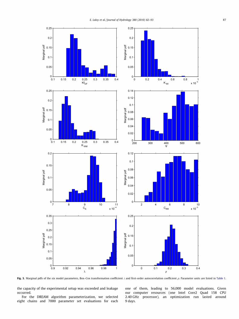
Fig. 2 shows the evolution of the R convergence criterion for thesix calibrated model parameters, k and q. It can be seen that 35,000objective function evaluations were necessary to ensure conver-gence within the chains to a stable distribution of pðb; k;qjbY; xÞðR < 1:2Þ. Given the selected number of chains (8) and modelevaluations (56,000), 21,000 parameter sets were sampled fromthe stable posterior parameter distribution.

Histograms of Fig. 3 are marginal posterior pdfs of the six modelparameters, k and q. Table 2 summarises the basic statistics ofthese marginal posterior pdfs together with the most likely param-eter value for each model parameter, k and q. Marginal posteriordistributions of hydraulic conductivity parameters KfOF ; KfWI andKfWM show a log-normal, slightly bimodal, shape and their poster-ior mean consequently does not match either their most likely va-lue or the optimal parameter value. However, given that the peakof their posterior pdf around the most likely value is sharp, theseparameters are well defined for the studied area. The most likelyvalue of the CK soil stability parameter is well defined but its pos-terior distribution is also slightly bimodal. The optimized distribu-tions of W and CRR have relatively irregular shapes indicating alarge uncertainty on their most likely value. Moreover, W and CRR

posterior distributions still have a large probability at their upperbounds despite the fact that the latter represent reasonable phys-ical limits. Indeed, the upper limit for W is typical of sandy loamsoils (Rawls et al., 1983). Furthermore, a value of CRR in excess ofthe upper limit would result in an unrealistically sharp decreaseof soil roughness as a function of cumulative rainfall kinetic en-ergy. One must also note that for all parameters, the range of thex-axes are narrower than the intervals between the lower andupper bounds selected for the optimization process (Table 1).

Table 2 indicates that moderate to strong linear correlations ex-ist between model parameters except CRR. Some of the correlationsbetween parameters are directly explained by their effect on modelresponse. Indeed, a decrease of KfOF ; KWI; KWM and W will have thesame global effect on model response than an increase of CRR andCK : a greater runoff production. For this reason, the hydraulic con-ductivity parameters KfOF (Fig. 4), KWI and KfWM (not shown) arenegatively correlated with W, and W and CK are positively corre-lated. In some cases, positive or negative correlations betweenparameters that have the same impact on model runoff productionare indirectly due to the existence of another strong correlation be-tween, on the one hand, the two considered parameters and, on theother hand, another parameter. KfOF , for example, is bound to CK

with a negative correlation coefficient of 0.97 (Fig. 4) despite thefact that an increase of KfOF or a decrease of CK will, in both cases,

reduce model runoff production. This is due to the fact that KfOF isalso strongly negatively correlated to W (correlation coefficient of�0.97) whereas W is positively correlated with CK (correlationcoefficient of 0.98). Given that the hydraulic conductivity parame-ters and W are both used to compute infiltration through theGreen–Ampt equation (see Laloy and Bielders, 2008), their strongnegative correlations suggest that W could be fixed based on theliterature.

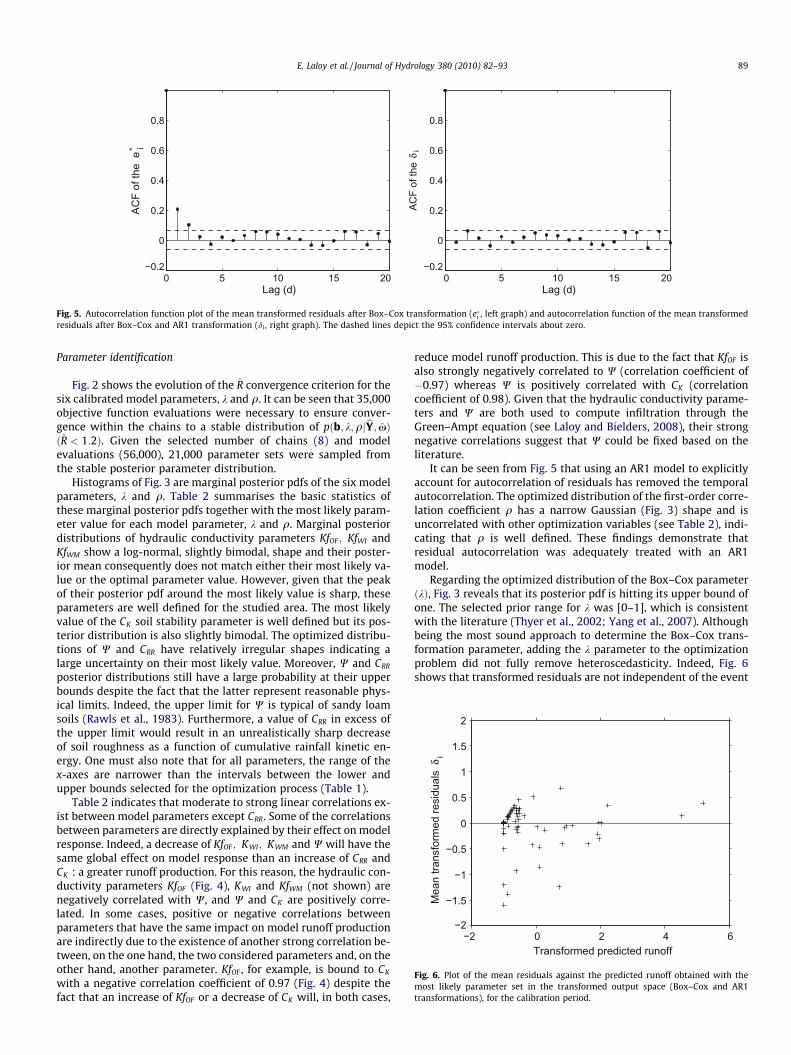
It can be seen from Fig. 5 that using an AR1 model to explicitlyaccount for autocorrelation of residuals has removed the temporalautocorrelation. The optimized distribution of the first-order corre-lation coefficient q has a narrow Gaussian (Fig. 3) shape and isuncorrelated with other optimization variables (see Table 2), indi-cating that q is well defined. These findings demonstrate thatresidual autocorrelation was adequately treated with an AR1model.

Regarding the optimized distribution of the Box–Cox parameterðkÞ, Fig. 3 reveals that its posterior pdf is hitting its upper bound ofone. The selected prior range for k was [0–1], which is consistentwith the literature (Thyer et al., 2002; Yang et al., 2007). Althoughbeing the most sound approach to determine the Box–Cox trans-formation parameter, adding the k parameter to the optimizationproblem did not fully remove heteroscedasticity. Indeed, Fig. 6shows that transformed residuals are not independent of the event

50 100 150 200 250 3000

50R

ainf

all (

mm

d−1

)

50 100 150 200 250 3000

2

4

6

8

Run

off (

mm

d−1

)

50 100 150 200 250 3000

2

4

6

8

Run

off (

mm

d−1

)

Time in the simulation (d)

Fig. 7. Hydrograph prediction uncertainty for the first year (2004–2005) of the calibration period (days 1–199 = intercropping subperiod, days 199–349 = maize subperiod).Observed daily runoff data are represented by a black dot. The light shaded area in the middle graph denotes the 95% total predictive uncertainty. The dark shaded area in thelower graph denotes the 95% prediction uncertainty that results from parameter uncertainty. The very light shaded rectangle cover a fraction of the period for which theexperimental setup was not operational (maize planting) and data are consequently unavailable.

90 E. Laloy et al. / Journal of Hydrology 380 (2010) 82–93

magnitude. In the most likely transformed output space, the cali-brated model tends to underpredict small to moderate runoffevents and slightly overestimate high runoff events. Assuming thatobservational input and output errors are negligible, this modelbehavior can be fully attributed to model structural inadequacyand suggest the need for model improvement. As discussed further,these runoff volume underestimations are often associated withthe beginnings of maize subseasons.

Uncertainty on predictions for the calibration and validation periods

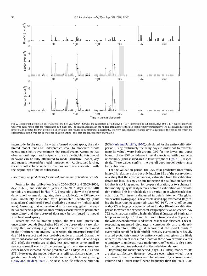
Results for the calibration (years 2004–2005 and 2005–2006,days 1–699) and validation (years 2006–2007, days 710–1040)periods are presented in Figs. 7–9. These plots show the observeddaily runoff volume during rainy days (black dots), the 95% predic-tion uncertainty associated with parameter uncertainty (darkshaded area) and the 95% total predictive uncertainty (light shadedarea). Assuming that observational errors are negligible, the gapsbetween the 95% prediction uncertainty associated with parameteruncertainty and the observed data may be attributed to modelstructural inadequacy.

Regarding the calibration period, the 95% total predictionuncertainty bounds (bracketing 96% of the observations) are rela-tively thin, indicating a good model performance. As mentionedin the ‘‘Optimization strategy” subsection, the measured runoff ofday 184 is suspect and very probably underestimated. During themaize subseasons of the calibration period (days 210–349 and days572–699), the results are slightly less accurate as some small tomoderate runoff events of the beginning of the maize season areeither underestimated, or not predicted at all (days 241, 573 and575). However, the model behavior is still satisfactory given thegreater complexity of such periods for which plants are growing(Laloy and Bielders, 2008). The Nash–Sutcliffe efficiency criterion

(NS) (Nash and Sutcliffe, 1970), calculated for the entire calibrationperiod (using exclusively the rainy days in order not to overesti-mate its value), were both around 0.92 for the lower and upperbounds of the 95% confidence interval associated with parameteruncertainty (dark shaded area in lower graphs of Figs. 7–9), respec-tively. These values confirm the overall good model performancefor calibration.

For the validation period, the 95% total predictive uncertaintyinterval is relatively thin but only brackets 83% of the observations,revealing that the error variance r2

d estimated from the calibrationdata is too low. This may be due to the use of a calibration data per-iod that is not long enough for proper calibration, or to a change inthe underlying system dynamics between calibration and valida-tion periods. This is probably due to a variation in wheel track char-acteristics. This issue is discussed in details later on. The globalshape of the hydrograph is nevertheless well approximated. Regard-ing the intecropping subperiod (days 700–917), the runoff volumeof day 722 is largely overpredicted. As for day 184 of the calibrationperiod for which the experimental setup capacity was exceeded, day722 was characterised by a high rainfall peak (measured 1-min rain-fall peak intensity of 108 mm h�1 and return period of 9 years forthe whole event duration) and water leakage was observed. The cor-responding measured discharge is consequently also underesti-mated. Therefore, although it seems that the model tends tooverpredict runoff for high rainfall intensity events on bare heavilycrusted plots, this cannot be entirely confirmed, given the likelyunderestimation of measured runoff for these two extreme events.A tendency to underestimate moderate runoff events is also notedfor the intecropping subperiod of the validation dataset.

Regarding the maize subperiod (days 943–1040), model resultsare also satisfactory. However, because even when wheel tracksare present, maize seasons are characterised by a lower runoffvolume and a lower runoff event frequency than the 2004–2005

400 450 500 550 600 6500

50R

ainf

all (

mm

d−1

)

400 450 500 550 600 6500

2

4

6

8

Run

off (

mm

d−1

)

400 450 500 550 600 6500

2

4

6

8

Run

off (

mm

d−1

)

Time in the simulation (d)

Fig. 8. Hydrograph prediction uncertainty for the second year (2005–2006) of the calibration period (days 366–563 = intercropping period, days 572–699 = maize period).Observed daily runoff data are represented by a black dot. The light shaded area in the middle graph denotes the 95% total predictive uncertainty. The dark area in the lowergraph denotes the 95% prediction uncertainty that results from parameter uncertainty. The very light shaded rectangle covers a fraction of the period for which theexperimental setup was not operational (maize planting) and data are consequently unavailable.

750 800 850 900 950 10000

50

Rai

nfal

l (m

m d

−1)

750 800 850 900 950 10000

2

4

6

8

Run

off (

mm

d−1

)

750 800 850 900 950 10000

2

4

6

8

Run

off (

mm

d−1

)

Time in the simulation (d)

Fig. 9. Hydrograph prediction uncertainty for the validation period (years 2006–2007, days 710–917 = intercropping period, days 943–1040 = maize period). Observed dailyrunoff data are represented by a black dot. The light shaded area in the middle graph denotes the 95% total predictive uncertainty. The dark shaded area in the lower graphdenotes the 95% prediction uncertainty that results from parameter uncertainty. The very light shaded rectangle covers a fraction of the period for which the experimentalsetup was not operational (maize planting) and data are consequently unavailable.

E. Laloy et al. / Journal of Hydrology 380 (2010) 82–93 91

92 E. Laloy et al. / Journal of Hydrology 380 (2010) 82–93

and 2006–2007 intercropping periods with heavily crusted soil andwheel tracks, more data would be needed to confirm the adequacyof model behavior during the maize cropping season. For the entirevalidation period, the NS criterion (computed by using exclusivelythe rainy days in order not to overestimate its value) associatedwith lower and upper bounds of the 95% confidence interval corre-sponding to parameter uncertainty were 0.76 and 0.78, respec-tively. These results show that the calibrated model may be usedwith a certain confidence for plot-scale, mid term and probablylong term (e.g., a few decades) simulation of the hydrological im-pact of different management practices in continuous maize crop-ping systems. The optimized model parameters (i.e., the mostsensitive ones on a daily basis, see Laloy et al., 2008) do not dependon the plant species but only on soil and tillage properties. To-gether with the satisfactory model performance, this leads us tobelieve that the model could relatively easily be extended to themid or long term evaluation of the hydrological impact of croppingpractices for other crops than maize. There is also no theoreticalreason that would prevent the upscaling of the model from plotto hillslope or even small catchment scale but, given that each typeof grid element requires an appropriate parameter set, this woulddramatically increase the number of parameters to be optimized.

When wheel tracks are present on the plot, their characteristicsare considered invariant throughout the entire simulation period(intercropping or maize period). This could partly explain the gapsbetween observations and predictions during the validation period(Fig. 9). Indeed, wheel track properties (width, random roughnessand hydraulic conductivity) may change depending, amongst oth-ers, on the wetness state of the soil at the time of wheel track cre-ation: maize harvest (wheel tracks of the bare 2004–2005 and2006–2007 intercropping periods) or maize planting (wheel tracksof the 2006 and 2007 maize seasons). Another source of discrep-ancy between observations and predictions could also be theintra-plot heterogeneity of the model parameters that the optimi-zation process lump into optimized parameter pdfs. Indeed, soilhydraulic conductivity parameters ðKfOF ; KfWI and KfWMÞ andGreen–Ampt soil matric potential ðWÞ are known to be highly spa-tially variable (Karssenberg, 2006), even at a 90 m2 scale.

Finally, Figs. 7–9 show that parameter uncertainty (dark shadedarea) accounts for a relatively minor part of total predictive uncer-tainty (light shaded area). The fact that the region associated withparameter uncertainty is relatively narrow but often does notbracket the observed data in the validation dataset indicates thatmodel structure and, probably to a lesser extent, observation mea-surements, are in need of further improvement.

Summary and conclusions

An efficient MCMC sampler, the Differential Evolution Adapta-tive Metropolis algorithm (DREAM: Vrugt et al., 2009a) has beensuccessfully used to calibrate in a Bayesian framework the contin-uous, spatially distributed, process-based and plot-scale runoffmodel described by Laloy and Bielders (2008). The calibration pro-cedure was corrected for heteroscedasticity (Box–Cox transforma-tion) and autocorrelation (AR1 model) of the residuals. Theoptimized value of the Box–Cox parameter did not fully removeheteroscedasticity but autocorrelation was adequately treatedwith the AR1 model. The method therefore resulted in a realisticestimation of parameter uncertainty and allowed, assuming thatobservational errors are negligible in our plot-scale context, to dif-ferentiate the impact of parameter uncertainty from the effect oftotal model error on model predictions.

Model results of the calibration period are very satisfactory forthe intercropping subperiods: the 95% total predictive uncertaintybounds are narrow. For the maize subperiods, results are slightly

less accurate. The Nash–Sutcliffe efficiency criterion associatedwith lower and upper bounds of the 95% confidence interval corre-sponding to parameter uncertainty only were both around 0.92 forthe entire calibration period. For the validation period, 17% of thepredictions are outside the 95% total predictive uncertaintybounds, possibly because the calibration period was too short tobe representative or because of a change of wheel track propertiesbetween calibration et validation periods.

Overall, the global shape of the hydrograph was reasonably wellapproximated. Furthermore, predictions relative to the maize sub-season seem satisfactory but more data are needed to confirm it.For the entire validation period, the Nash–Sutcliffe efficiency crite-rion associated with the lower and upper bounds of the 95% confi-dence interval corresponding to parameter uncertainty were 0.76and 0.78, respectively. These results show that the calibrated mod-el may be used with a certain confidence for plot-scale, mid termand probabily long term simulation of the hydrological impact ofdifferent management practices in continuous maize croppingsystems.

More generally, the 95% predictive uncertainty associated withparameter uncertainty was always very narrow. However, it oftendid not bracket the observations during the validation period, indi-cating that, assuming that observation errors are negligible, modelstructure has to be improved in order to achieve more accuratepredictions. In the future, an adequate explicit evaluation andtreatment of input and output measurement errors could allowfor a more precise evaluation of model structural errors whereasparallel computing could significantly reduce the currently highcalculation time.

Acknowledgements

This work was funded by the Direction générale de l’agriculture(DGA) of the Service Public de Wallonie (Belgium). The authors arethankful to Jasper Vrugt for his support when using the DREAMalgorithm. We also wish to thank three anonymous reviewers fortheir helpful comments.

References

Beven, K., Binley, A., 1992. The future of distributed models: model calibration andpredictive uncertainty. Hydrological Processes 6, 279–298.

Box, G., Cox, D., 1964. An analysis of transformations. Journal of the Royal StatisticalSociety Series B 26 (2), 211–252.

Box, G., Jenkins, G., 1976. Time Series Analysis: Forecasting and Control. Holden-Day, San Francisco, USA.

Box, G., Tiao, G., 1973. Bayesian Inference in Statistical Analysis. Addison-Wesley,Reading, MA, USA.

Chow, V.T., Maidment, D.R., Mays, L.W., 1988. Applied Hydrology. McGraw-Hill,New York, USA.

Chu, S.T., 1978. Infiltration during an unsteady rain. Water Resources Research 14(3), 461–466.

Cooper, V., Nguyen, V.-T.-V., Nicell, J., 2007. Calibration of conceptual rainfall–runoffmodels using global optimization methods with hydrologic process-basedparameter constraints. Journal of Hydrology 334, 455–466.

Duan, Q., Sorooshian, S., Gupta, V., 1992. Effective and efficient global optimizationfor conceptual rainfall–runoff models. Water Resources Research 28 (4), 1015–1031.

Fankhauser, R., 1997. Measurement properties of tipping bucket recording raingages and their influence on urban runoff simulation. Water Science andTechnology 36 (8), 7–12.

Feyen, L., Vrugt, J., Ó Nualláin, B., van der Knijff, J., De Roo, A., 2007. Parameteroptimization and uncertainty assessment for large scale streamflow simulationwith the LISFLOOD model. Journal of Hydrology 332, 276–289.

Gallagher, M., Doherty, J., 2007. Parameter estimation and uncertainty analysis for awatershed model. Environmental Modelling & Software 22, 1000–1020.

Gelman, A., Rubin, D.B., 1992. Inference from iterative simulation using multiplesequences. Statistical Science 7, 457–472.

Gelman, A., Carlin, J.B., Stren, H.S., 1995. Bayesian Data Analysis. Chapmann andHall, New YorkUSA.

Georgakakos, K.P., Seo, D.-J., Gupta, H., Schaake, J., Butts, M.B., 2004. Towards thecharacterization of streamflow simulation uncertainty through multimodelensembles. Journal of Hydrology 298, 222–241.

E. Laloy et al. / Journal of Hydrology 380 (2010) 82–93 93

Green, W., Ampt, G., 1911. Studies on soil physics: 1, flow of air and water throughsoils. Journal of Agricultural Science 4, 1–24.

Hastings, W.K., 1970. Monte Carlo sampling methods using Markov Chains andtheir applications. Biometrika 57, 97–109.

Iorgulescu, I., Beven, K.J., Musy, A., 2005. Data-based modelling of runoff andchemical tracer concentrations in the Haute–Mentue research catchment(Switzerland). Hydrological Processes 19 (13), 2557–2573.

Karssenberg, D., 2006. Upscaling of saturated conductivity for Hortonian runoffmodelling. Advances in Water Resources 14 (3), 461–466.

Kuczera, G., 1983. Improved parameter inference in catchment models. 1.Evaluating parameter uncertainty. Water Resources Research 19 (5), 1151–1162.

Kuczera, G., Mroczkowski, M., 1998. Assessment of hydrologic parameteruncertainty and the worth of multi-response data. Water Resources Research34 (6), 1481–1490.

Kuczera, G., Parent, E., 1998. Monte Carlo assessment of parameter uncertainty inconceptual catchment models: the Metropolis algorithm. Journal of Hydrology211, 69–85.

Laloy, E., Bielders, C., 2008. Plot scale continuous modelling of runoff in a maizecropping system with dynamic soil surface properties. Journal of Hydrology349, 455–469.

Laloy, E., Bielders, C.L., 2009a. Modelling intercrop management impact on runoffand erosion in a continuous maize cropping system: part I. Model description,global sensitivity analysis and Bayesian estimation of parameter identifiability.European Journal of Soil Science 60, 1005–1021.

Laloy, E., Bielders, C.L., 2009b. Modelling intercrop management impact onrunoff and erosion in a continuous maize cropping system: part II.Model Pareto multiobjective calibration and long term scenario analysisusing disaggregated rainfall. European Journal of Soil Science 60, 1022–1037.

Metropolis, N., Rosenbluth, A.W., Rosenbluth, M.N., Teller, A.H., 1953. Equations ofstate calculations by fast computing machines. Journal of Chemical Physics 21,1087–1091.

Molini, A., Lanza, L.G., La Barbera, P., 2005. Improving the accuracy of tipping-bucketrain records using disaggregation techniques. Atmospheric Research 77, 203–207.

Nash, J., Sutcliffe, J., 1970. River flow forecasting through conceptual models, 1, adiscussion of principles. Journal of Hydrology 10 (1), 282–290.

Rawls, W., Brakensiek, D., Miller, N., 1983. Green–Ampt infiltration parameters fromsoil data. Journal of Hydraulic Engineering – ASCE 109 (1), 62–70.

Schaefli, B., Talamba, B.D., Musy, A., 2007. Quantifying hydrological modeling errorsthrough a mixture of normal distributions. Journal of Hydrology 332, 303–315.

Sorooshian, S., Dracup, J., 1980. Stochastic parameter estimation procedures forhydrological rainfall–runoff models: correlated and heteroscedastic errors.Water Resources Research 16 (2), 430–442.

Stransky, D., Bares, V., Fatka, P., 2007. The effect of rainfall measurementuncertainties on rainfall–runoff processes modelling. Water Science andTechnology 55 (4), 103–111.

Sumner, N., Fleming, P., Bates, B., 1997. Calibration of a modified SFB model fortwenty-five Australian catchments using simulated annealing algorithms.Journal of Hydrology 197, 166–188.

Thyer, M., Kuczera, G., Wang, Q.J., 2002. Quantifying parameter uncertainty instochastic models using the Box–Cox transformation. Journal of Hydrology 265,246–257.

Uhlenbrook, S., Seibert, J., Leibundgut, C., Rhode, A., 1999. Prediction uncertainty ofconceptual rainfall–runoff models caused by problems in identifying modelparameters and structure. Hydrological Sciences Journal 44, 779–797.

Verhulst, P.F., 1845. Mathematical researches into the law of population growthincrease. Nouveaux Mémoires de l’Académie Royale des Sciences et Belles-Lettres de Bruxelles 18, 1–45.

Vrugt, J., Boutem, W., 2002. Validity of first-order approximations to describeparameter uncertainty in soil hydrologic models. Soil Science Society ofAmerica Journal 66, 1740–1751.

Vrugt, J.A., Robinson, B.A., 2007. Improved evolutionary optimization fromgenetically adaptative multimethod search. Proceedings of the NationalAcademy of Sciences of the United States of America 104, 708–711.

Vrugt, J., Gupta, H., Bouten, W., Sorooshian, S., 2003. A shuffled complex evolutionmetropolis algorithm for optimization and uncertainty assessment ofhydrologic parameter estimation. Water Resources Research 39 (8), 1201.doi:10.1029/2002WR001642.

Vrugt, J., Ter Braak, C., Clarke, M., Hyman, J., Robinson, B., 2009a. Treatment of inputuncertainty in hydrologic modeling: doing hydrology backwards with MarkovChain Monte Carlo simulation. Water Resources Research 44, W00B09.doi:10.1029/2007WR006720.

Vrugt, J., Ter Braak, C., Gupta, H., Robinson, B., 2009b. Equifinality of formal(DREAM) and informal (GLUE) Bayesian approaches in hydrologic modeling.Stochastic Environmental Research and Risk Assessment, 1–3. doi:10.1007/s00477-008-0284-9.

Vrugt, J., Ter Braak, C., Diks, C., Robinson, B., Hyman, J., Higdon, D., 2009c.Accelerating Markov Chain Monte Carlo simulation using self-adaptativedifferential evolution with randomized subspace sampling. InternationalJournal of Nonlinear Sciences and Numerical Simulation 10 (3), 1–12.

Yang, J., Reichert, P., Abbaspour, K.C., Yang, H., 2007. Hydrological modelling of theChaohe Basin in China: statistical model formulation and Bayesian inference.Journal of Hydrology 340, 167–182.