parameter estimation methods for ordinary di …...parameter estimation methods for ordinary di...
TRANSCRIPT

Parameter Estimation Methods for Ordinary Differential Equation
Models with Applications to Microbiology
Justin M. Krueger
Dissertation submitted to the Faculty of the
Virginia Polytechnic Institute and State University
in partial fulfillment of the requirements for the degree of
Doctor of Philosophy
in
Mathematics
Matthias Chung, Chair
Julianne Chung
Serkan Gugercin
Mihai Pop
July 21, 2017
Blacksburg, Virginia
Keywords: Parameter Estimation, Ordinary Differential Equations, Microbiota,
Least-Squares Finite Element Method
Copyright 2017, Justin M. Krueger

Parameter Estimation Methods for Ordinary Differential Equation
Models with Applications to Microbiology
Justin M. Krueger
(ABSTRACT)
The compositions of in-host microbial communities (microbiota) play a significant role in
host health, and a better understanding of the microbiota’s role in a host’s transition from
health to disease or vice versa could lead to novel medical treatments. One of the first steps
toward this understanding is modeling interaction dynamics of the microbiota, which can be
exceedingly challenging given the complexity of the dynamics and difficulties in collecting
sufficient data. Methods such as principal differential analysis, dynamic flux estimation, and
others have been developed to overcome these challenges for ordinary differential equation
models. Despite their advantages, these methods are still vastly underutilized in math-
ematical biology, and one potential reason for this is their sophisticated implementation.
While this work focuses on applying principal differential analysis to microbiota data, we
also provide comprehensive details regarding the derivation and numerics of this method.
For further validation of the method, we demonstrate the feasibility of principal differential
analysis using simulation studies and then apply the method to intestinal and vaginal mi-
crobiota data. In working with these data, we capture experimentally confirmed dynamics
while also revealing potential new insights into those dynamics. We also explore how we find
the forward solution of the model differential equation in the context of principal differential
analysis, which amounts to a least-squares finite element method. We provide alternative
ideas for how to use the least-squares finite element method to find the forward solution and
share the insights we gain from highlighting this piece of the larger parameter estimation
problem.
Parameter Estimation Methods for Ordinary Differential Equation
Models with Applications to Microbiology
Justin M. Krueger
(GENERAL AUDIENCE ABSTRACT)
In this age of “big data,” scientists increasingly rely on mathematical models for analyzing
the data and drawing insights from them. One particular area where this is especially true
is in medicine where researchers have found that the naturally occurring bacteria within
individuals play a significant role in their health and well-being. Understanding the bacteria’s
role requires that we understand their interactions with each other and with their hosts so
that we can predict how changes in bacterial populations will affect individuals’ health. Given
the number and complexity of these interactions, creating good models for them is a difficult
task that traditional methods often fail to complete. The goal of this work is to promote the
awareness of alternatives to the traditional modeling methods and to present a particular
alternative in a way that is accessible to readers to encourage its and other methods’ use.
With this goal and the medical application as the focus of our work, we discuss some of
the traditional methods for constructing such models, discuss some of the more modern
alternatives, and describe in detail the method we use. We explain the derivation of the
method and apply it to both an example problem and two separate experimental studies to
demonstrate its usefulness, and in the case of the experimental studies, we gain interesting
insights into the bacterial interactions captured by the data. We then focus on some of
the method’s numerical details to further highlight its strengths and to identify how we can
improve its application.

Dedicated to my family and friends.
iv

Acknowledgments
I do not think I can adequately express how much of a collective group effort completing
this dissertation was, but I hope that I can properly express my gratitude to everyone who
played a role.
I would first like to thank the National Institute Of General Medical Sciences of the National
Institutes of Health for their funding of this work under award number R21GM107683-01.
Your support gave me the time and resources to complete much of this research.
I also want to acknowledge the Virginia Tech Department of Mathematics. I always enjoyed
the familial atmosphere you, the faculty and staff, fostered, and the kindness you consistently
showed me never went unnoticed.
Within the department, I would specifically like to mention my adviser, Dr. Matthias Chung.
I am so grateful for the guidance, insights, and opportunities you provided me, and I feel
incredibly privileged because I know not all graduate students are so lucky.
I would also like to thank my committee, Drs. Julianne Chung, Serkan Gugercin, and Mihai
Pop. Learning from you through seminars, classes, and collaborations was an invaluable
experience, and I appreciate the feedback and support you gave me.
I must recognize my classmates, especially Sam Erwin, Kasie Farlow, Holly Grant, Kelli
Karcher, and George Kuster. Your camaraderie throughout the daily grind of graduate
v

school influenced my experience for the better, and I hope I did the same for you.
I additionally want to thank my friends from the Newman community, specifically Katelyn
Catalfamo, Darien and Clara Clark, Zach and Lauren DeSmit, Patrick and Emily Good, Jon
and Julianna Hellmann, Eric Johannigmeier, John and Mary Beth Keenan, and Mark and
Katelyn Mazzochette. You brought me joy in the times when I needed it the most, and you
added purpose to my time at Virginia Tech.
I would also like to express my gratitude to my family. Mom and Dad, you never let me
settle for anything short of my best, and when my own expectations of graduate school
overwhelmed me, you were always there to help me see it through to the end. Laura and
Sara, your relentless pursuit of your own aspirations challenged me to be better, yet you
were always able to keep me grounded in ways only you could. Thank you to all of you for
being there every step of the way.
Finally, I must express my love and appreciation to Jilian, my wife and best friend. The last
seven years were not just about this dissertation but about building the foundations of our
own story. You were by my side for the entirety of this work, and I could not have done it
without you. As we close this chapter of our life, I cannot wait to see what new adventures
life brings next, and I look forward to sharing them all with you.
vi

Contents
List of Figures xi
1 Introduction 1
1.1 Motivation . . . . . . . . . . . . . . . . . . . . . . . . . . . . . . . . . . . . . 1
1.2 Outline . . . . . . . . . . . . . . . . . . . . . . . . . . . . . . . . . . . . . . . 2
2 Background 4
2.1 Ordinary Differential Equations . . . . . . . . . . . . . . . . . . . . . . . . . 4
2.2 Numerical Methods for Ordinary Differential Equations . . . . . . . . . . . . 6
2.3 Applications of Ordinary Differential Equations . . . . . . . . . . . . . . . . 8
2.4 Parameter Estimation for Ordinary Differential Equations . . . . . . . . . . 9
3 Parameter Estimation for Microbiota Models 11
3.1 Introduction . . . . . . . . . . . . . . . . . . . . . . . . . . . . . . . . . . . . 11
3.1.1 Biology of Microbiota . . . . . . . . . . . . . . . . . . . . . . . . . . . 11
3.1.2 Lotka-Volterra Model . . . . . . . . . . . . . . . . . . . . . . . . . . . 13
vii
3.1.3 Model Assumptions . . . . . . . . . . . . . . . . . . . . . . . . . . . . 14
3.2 Methods . . . . . . . . . . . . . . . . . . . . . . . . . . . . . . . . . . . . . . 16
3.2.1 Problem Statement . . . . . . . . . . . . . . . . . . . . . . . . . . . . 16
3.2.2 Single Shooting Methods . . . . . . . . . . . . . . . . . . . . . . . . . 17
3.2.3 Alternative Methods . . . . . . . . . . . . . . . . . . . . . . . . . . . 18
3.2.4 Principal Differential Analysis . . . . . . . . . . . . . . . . . . . . . . 20
3.2.5 Computational Details . . . . . . . . . . . . . . . . . . . . . . . . . . 22
3.3 Results and Discussion . . . . . . . . . . . . . . . . . . . . . . . . . . . . . . 26
3.3.1 Simulation Studies . . . . . . . . . . . . . . . . . . . . . . . . . . . . 26
3.3.2 Intestinal Microbiota Dynamics . . . . . . . . . . . . . . . . . . . . . 30
3.3.3 Vaginal Microbiota Dynamics . . . . . . . . . . . . . . . . . . . . . . 34
3.4 Conclusions . . . . . . . . . . . . . . . . . . . . . . . . . . . . . . . . . . . . 38
4 Least-Squares Finite Element Method 41
4.1 Introduction . . . . . . . . . . . . . . . . . . . . . . . . . . . . . . . . . . . . 41
4.2 Methods . . . . . . . . . . . . . . . . . . . . . . . . . . . . . . . . . . . . . . 42
4.2.1 Problem Statement . . . . . . . . . . . . . . . . . . . . . . . . . . . . 42
4.2.2 Function Approximation . . . . . . . . . . . . . . . . . . . . . . . . . 44
4.2.3 Integral Norm Discretization . . . . . . . . . . . . . . . . . . . . . . . 45
4.2.4 Adaptive Schemes . . . . . . . . . . . . . . . . . . . . . . . . . . . . . 46
viii

4.3 Results and Discussion . . . . . . . . . . . . . . . . . . . . . . . . . . . . . . 47
4.3.1 Linear Initial Value Problem . . . . . . . . . . . . . . . . . . . . . . . 48
4.3.2 Two State Linear Initial Value Problem . . . . . . . . . . . . . . . . . 49
4.3.3 Nonlinear Initial Value Problem . . . . . . . . . . . . . . . . . . . . . 51
4.3.4 Piecewise Linear Initial Value Problem . . . . . . . . . . . . . . . . . 52
4.3.5 Six State Linear Initial Value Problem . . . . . . . . . . . . . . . . . 55
4.4 Conclusions . . . . . . . . . . . . . . . . . . . . . . . . . . . . . . . . . . . . 56
5 Conclusions and Future Research 58
5.1 Conclusions . . . . . . . . . . . . . . . . . . . . . . . . . . . . . . . . . . . . 58
5.2 Future Work . . . . . . . . . . . . . . . . . . . . . . . . . . . . . . . . . . . . 59
Bibliography 60
Appendices 71
Appendix A Parameter Estimation Details 72
A.1 Lotka-Volterra Model and Sparsity Constraint . . . . . . . . . . . . . . . . . 72
A.2 Simulation Studies . . . . . . . . . . . . . . . . . . . . . . . . . . . . . . . . 74
A.3 Intestinal Microbiota . . . . . . . . . . . . . . . . . . . . . . . . . . . . . . . 75
A.4 Vaginal Microbiota . . . . . . . . . . . . . . . . . . . . . . . . . . . . . . . . 76
Appendix B Approximating Function Details 78
ix

B.1 Quadratic Splines . . . . . . . . . . . . . . . . . . . . . . . . . . . . . . . . . 78
B.1.1 Quadratic Spline Definition . . . . . . . . . . . . . . . . . . . . . . . 78
B.1.2 Quadratic Spline Derivatives . . . . . . . . . . . . . . . . . . . . . . . 81
B.2 Cubic Splines . . . . . . . . . . . . . . . . . . . . . . . . . . . . . . . . . . . 82
B.2.1 Cubic Spline Definition . . . . . . . . . . . . . . . . . . . . . . . . . . 82
B.2.2 Cubic Spline Derivatives . . . . . . . . . . . . . . . . . . . . . . . . . 85
B.3 Exponential Splines . . . . . . . . . . . . . . . . . . . . . . . . . . . . . . . . 86
B.3.1 Exponential Spline Definition . . . . . . . . . . . . . . . . . . . . . . 86
B.3.2 Exponential Spline Derivatives . . . . . . . . . . . . . . . . . . . . . . 90
B.4 Hermite Cubic Splines . . . . . . . . . . . . . . . . . . . . . . . . . . . . . . 91
B.4.1 Hermite Cubic Spline Definition . . . . . . . . . . . . . . . . . . . . . 91
B.4.2 Hermite Cubic Spline Derivatives . . . . . . . . . . . . . . . . . . . . 92
x
List of Figures
3.1 Numerical solution of a Lotka-Volterra system from t = 0 to t = 200. . . . . 27
3.2 Simulated data points from the numerical solution of a Lotka-Volterra system. 27
3.3 Absolute errors of optimal model parameters and initial conditions for simu-
lation studies. . . . . . . . . . . . . . . . . . . . . . . . . . . . . . . . . . . . 28
3.4 Relative error between spline approximations and numerical solutions for sim-
ulation studies. . . . . . . . . . . . . . . . . . . . . . . . . . . . . . . . . . . 29
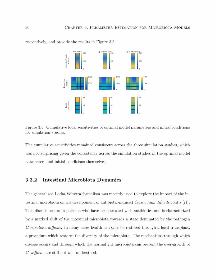
3.5 Cumulative local sensitivities of optimal model parameters and initial condi-
tions for simulation studies. . . . . . . . . . . . . . . . . . . . . . . . . . . . 30
3.6 Relative error between spline approximations and numerical solutions for in-
testinal microbiota model. . . . . . . . . . . . . . . . . . . . . . . . . . . . . 32
3.7 Comparison of numerical solutions for intestinal microbiota model. . . . . . . 32
3.8 Comparison of interaction matrices for intestinal microbiota model. . . . . . 33
3.9 Cumulative local sensitivities of optimal model parameters and initial condi-
tions for intestinal microbiota model. . . . . . . . . . . . . . . . . . . . . . . 34
xi

3.10 Relative error between spline approximations and numerical solutions for vagi-
nal microbiota model. . . . . . . . . . . . . . . . . . . . . . . . . . . . . . . . 35
3.11 Comparison of numerial solutions to data for vaginal microbiota model. . . . 36
3.12 Optimal interaction matrix for vaginal microbiota model. . . . . . . . . . . . 37
3.13 Cumulative local sensitivities of optimal model parameters and initial condi-
tions for vaginal microbiota model. . . . . . . . . . . . . . . . . . . . . . . . 38
3.14 Numerical solutions from day 0 to day 500 for vaginal microbiota model. . . 38
4.1 Solutions of linear initial value problem. . . . . . . . . . . . . . . . . . . . . 48
4.2 Solutions of two state linear initial value problem. . . . . . . . . . . . . . . . 49
4.3 Solutions of two state linear boundary value problem. . . . . . . . . . . . . . 51
4.4 Solutions of nonlinear initial value problem. . . . . . . . . . . . . . . . . . . 52
4.5 Solutions of piecewise linear initial value problem. . . . . . . . . . . . . . . . 53
4.6 Adaptive solutions of piecewise linear initial value problem. . . . . . . . . . . 54
4.7 Solutions of six state linear initial value problem. . . . . . . . . . . . . . . . 56
xii
Chapter 1
Introduction
1.1 Motivation
In a 2009 publishing of an internal memo [66], then Google senior vice president Jeff Rosen-
berg said, “Data is the sword of the 21st century, those who wield it well, the Samurai.” In
the eight years since, the collection, analysis, and exchange of data have exploded as a means
of profit for company’s like Google but have also become an invaluable tool in the pursuit of
knowledge. As the size and efficiency of data collection improves though, our ability to use
and analyze data increases in importance.
Constructing and fitting mathematical models via parameter estimation are two particular
areas where data analysis are important because these models allow us to study and exper-
iment without expending the limited material resources used to collect the data. Many of
these models rely on systems of ordinary differential equations to represent the dynamics
the data capture, and the model equations have the potential to be both large in scale and
chaotic in behavior. This means the traditional solution methods on which we often rely fail,
1

2 Chapter 1. Introduction
so we require robust methods that address the shortcomings of these traditional approaches.
With this as motivation, our work focuses on providing a viable alternative to these tradi-
tional methods. We first identify a method for ordinary differential equation models that
simultaneously estimates model parameters and solves the differential equation. This ap-
proach is a specific instance of a method called principal differential analysis, which is un-
derutilized in application, so we demonstrate its usefulness through simulation studies and
interesting insights when the method is applied to collected and published data on microbial
communities.
We then attempt to improve on this method by focusing on the piece that solves the differ-
ential equation. This focus amounts to working with least-squares finite element methods,
which are a popular tool for solving partial differential equations but are underutilized when
solving ordinary differential equations. We demonstrate that this approach can provide accu-
rate numerical solutions where other numerical methods fail, and we show that the approach
can compete with traditional methods when comparing computational efficiency.
Our contribution to this field is the detailed derivations and explanations in the chapters and
appendices that follow. Our hope is that this work will make these alternative, underutilized
computational methods more accessible and create a few more “Samurai” in the process.
1.2 Outline
In Chapter 2 we introduce the basic ideas necessary to contextualize our work. We start with
an overview of ordinary differential equations and the basic numerical methods used to solve
them. We then further discuss the application of ordinary differential equations to math-
ematical models, and we close the chapter by formulating the basic parameter estimation

1.2. Outline 3
problem.
Chapter 3 focuses on parameter estimation for biological systems. We discuss various param-
eter estimation methods that use finite element or finite difference techniques and compare
them to a version of principal differential analysis, which is our method of choice. We validate
our approach using simulation studies and then use two experimental data sets to further
demonstrate the benefits of our method. The majority of this chapter is also available as a
preprint [23], and we have submitted the entire chapter for publication [24].
Chapter 4 analyzes the part of principal differential analysis that solves the model differential
equation, which is a least-squares finite element method. We compare the least-squares finite
element method to finite difference methods and other finite element methods and provide
examples to highlight the competitive speed and robustness of the least-squares finite element
method compared to these other methods. We also discuss how we could apply some of the
insights from this chapter to the larger parameter estimation problem discussed in Chapter 3.
Chapter 5 then provides a conclusion to this work. We include a summary in which we
identify the points of emphasis and key insights of our work and a section on the relevant
questions and ideas we would like to pursue next.
Chapter 2
Background
2.1 Ordinary Differential Equations
A differential equation is a mathematical expression that relates a quantity of interest and
its derivatives. If the quantity of interest y is a function of a single independent variable t, we
call the differential equation ordinary, which is the type of differential equation we focus on
here. If the the relationship between y and its derivatives depends on the first r derivatives,
we call the differential equation rth order [46] and can express it as
y(r)(t) = f(t, y(t), y′(t), . . . , y(r−1)(t)).
The expression as it is written assumes that y is one-dimensional, but we can extend this
to the case where y is multi-dimensional. Regardless of the dimension of y or the order of
the differential equation, we can rewrite the expression as a system of first-order differential
equations
y′ = f(t,y) (2.1)
4
2.1. Ordinary Differential Equations 5
by changing the variable and dropping the explicit dependence on t. In this expression
y = [y1; . . . ; yn] ∈ Rn and f(·, ·) is a vector function.
We can pair (2.1) with additional restrictions on y. If the restrictions on y all depend on the
same value of t, e.g., y(t0) = y0, where t0 and y0 are known, then we call the combination
of (2.1) and these restrictions an initial value problem. If the restrictions on y depend on
two values of t, e.g., t0 and t1, then we call the combination of (2.1) and these restrictions a
boundary value problem [46].
The reason for this pairing is that differential equations often have infinitely many solutions,
but we often have interest in a specific solution on a specific interval of t. It is important
for us to know if such a solution exists and if it is unique, and for initial value problems, we
have the following theorem.
Theorem 2.1. Consider the initial value problem
y′ = f(t,y), y(t0) = y0,
where the initial value point (t0,y0) lies in the region R defined by a < t < b, αi < yi < βi,
i = 1, . . . , n. Let fj and∂fj∂yk
, j = 1, . . . , n, k = 1, . . . , n be continuous in R. Then the initial
value problem has a unique solution y(t) that exists on some t-interval (c, d) containing t0.
[46]
Existence and uniqueness theorems for boundary value problems do exist, but they rely on
special cases and are not as straightforward as Theorem 2.1.

6 Chapter 2. Background
2.2 Numerical Methods for Ordinary Differential Equa-
tions
Even if we know unique solutions exist, most differential equations do not have solutions we
can find analytically, so we find numerical approximations. For initial value problems, two
approximating techniques are finite difference methods and finite element methods.
With finite difference methods we discretize the t-interval of interest and approximate the
derivative in (2.1) with a difference equation. Using the initial conditions as a starting point,
we iteratively approximate the value of the solution at the discretization points [2].
While the outline is the same for all finite difference methods, we can classify specific finite
difference methods based on the details of their derivations. Two classification types are
one-step versus multi-step methods and explicit versus implicit methods.
One-Step Methods versus Multi-Step Methods. One-step methods use information
about a single discretization point to approximate the solution at a discretization point,
whereas multi-step methods use information about multiple discretization points to ap-
proximate the solution at a discretization point.
Explicit Methods versus Implicit Methods. Explicit methods rely on information about
previous discretization points, whereas implicit methods rely on information at the
current discretization point and can require solving a nonlinear system of algebraic
equations at every iteration.
Finite difference methods can differ in other ways. Some methods make use of approximations
to the solution at intermediate steps between discretization points, which are called stages, to
approximate the solution at a discretization point. Some methods adapt the discretization of
2.2. Numerical Methods for Ordinary Differential Equations 7
the t-interval at each iteration [2]. Regardless of the exact method, finite difference methods
provide an approximation to the solution at a finite number of points, and we must use
additional tools, such as interpolation, to approximate the solution elsewhere.
Finite element methods take a different approach to approximating the solution. With finite
element methods we discretize the t-interval of interest, but rather than approximate the
derivative with a difference equation, we approximate the solution on each subinterval, or
element, by a simpler function [74]. The type of simple function we choose in finite elements
has two crucial considerations.
Practicality. The solution of a differential equation is an element of an infinite dimensional
vector space, so we restrict our approximating function to one that is an element of a
finite dimensional vector space. That is, we can define the approximating function by
choosing a finite number of parameters like the function’s coefficient values.
Continuity Conditions. The solution to a differential equation is at least differentiable so
the approximating function should also be differentiable. In some cases, we identify
additional continuity conditions for a solution of a differential equation, and we should
choose an approximating function that reflects those conditions as well.
As with the finite difference methods, finite element methods can differ based on their deriva-
tions. For example, we can build finite element methods based on the Rayleigh-Ritz Principle
or the Galerkin Principle [74]. Regardless of the exact method, finite element methods pro-
vide an approximation to the solution over the entire t-interval, which means we require no
additional tools like interpolation to approximate the solution at certain points.
8 Chapter 2. Background
2.3 Applications of Ordinary Differential Equations
Because differential equations relate quantities of interest to their derivatives and this type
of relationship occurs naturally, they have many applications across many subjects. Here
are a few examples.
Physics. We can describe the motion of a falling object that experiences air resistance
proportional to its velocity by the first order differential equation
mv′ = −mg − kv,
where m is the object’s mass, g is the acceleration due to gravity, k is the drag constant,
and v is the object’s velocity [46].
Chemistry. Michaelis-Menten kinetics describe enzymatic reactions usng the first order
differential equation
[P ]′ =Vmax[S]
KM + [S].
In this equation [P ] is the concentration of the reaction product, [S] is concentration
of the reaction substrate, Vmax is the maximum reaction rate, and KM is the Michaelis
constant, which is the substrate concentration at which the reaction rate is 50 percent
of Vmax [53].
Economics. The Solow-Swan model is an economic growth model that depends on capital
accumulation, labor growth, and increases in productivity. One part of the model is
the first order differential equation
k′ = sf(k)− (n+ g + δ)k,

2.4. Parameter Estimation for Ordinary Differential Equations 9
where k is the capital stock per unit of effective labor, f(k) is the output per unit of
effective labor, s is the fraction of the output that is saved for investment, n is the
growth rate of labor, g is the growth rate of knowledge, and δ is the capital depreciation
rate [70].
Biology. We can describe the population growth rate of a particular species using the first
order differential equation
P ′ = rP
(1− P
K
),
where P is the species’ population, r is its the growth rate, and K is the carrying
capacity [81, 82].
The significance of these example models is to show that differential equations, their param-
eters, and their solutions often have physical meaning, and studying these models can lead
to quantitative insights about the applications.
2.4 Parameter Estimation for Ordinary Differential Equa-
tions
To gain physical insights about the applications like those listed in Section 2.3, we first
need to know the model parameters. We know or can easily determine the value of some
parameters, but this is not true in general. We instead observe the quantity of interest or
a representation of it as experimental data, which gives a snapshot of the solution of the
differential equation that we use determine appropriate values for the the parameters.
Rewriting (2.1) to explicitly show dependence on its parameters p and adding initial condi-

10 Chapter 2. Background
tions gives
y′ = f(t,y; p), y(a) = y0,
and determining the values of the parameters is equivalent to solving the optimization prob-
lem
minpJ(y,d)
subject to y′ = f(t,y; p), a < t < b,
y(a) = y0,
where J is a nonnegative measure of the error between the solution of the differential equation
y given p and the experimental data d. This is the basis of parameter estimation for ordinary
differential equations.
Chapter 3
Parameter Estimation for Microbiota
Models
3.1 Introduction
3.1.1 Biology of Microbiota
Bacteria are ubiquitous in our world and play a key role in maintaining the health of our
environment as well as the health of virtually all living organisms. The human-associated
microbial communities (microbiota) have been shown to be at least associated with, if not
causative of, several human diseases such as periodontitis [50], type 2 diabetes [60], atopic
dermatitis [47], ulcerative colitis [87], Crohn’s disease [51], and vaginosis [62]. Furthermore,
time series data have shown that the host-associated microbiota undergo dynamic changes
over time within the same individual, e.g., within the gut of a developing infant [45, 56],
the gut, mouth, and skin of healthy adults [18], and within the vagina of reproductive age
women [29]. The mechanisms that underlie these changes are currently not well understood,
11
12 Chapter 3. Parameter Estimation for Microbiota Models
whether they represent fluctuations in the normal flora or the transition from health to
disease and conversely from disease to health after treatment.
Understanding the role human-associated microbiota play in health and disease requires
the elucidation of the complex networks of interactions among the microbes and between
microbes and the host, which is a challenging task due to our inability to directly observe
bacterial interactions. Researchers have reconstructed microbial networks based on indirect
approaches, such as knowledge about the metabolic functions encoded in the genomes of
the interacting partners [49], coexistence patterns across multiple samples [19], covariance
of abundance across samples [28], or changes in abundance across time [67, 71]. Multiple
mathematical formalisms have been used to reason about the resulting networks with ex-
amples including metabolic modeling through flux balance analysis [73], machine learning
algorithms based on environmental parameters [31], and differential equation based models
of interactions [71].
Here we focus on the latter, a flexible formalism that can model complex interaction pat-
terns, including abundance-dependent interaction parameters [78]. While such modeling
approaches have been developed since the 1980s in the context of wastewater treatment sys-
tems [39], their use in studying human-associated microbiota has been limited, in no small
part due to the specific characteristics of human microbiome data. First, the rate at which
samples can be collected is severely limited by clinical and logistical factors, e.g., stool sam-
ples can be collected roughly on a daily basis, while subgingival plaque may only be feasibly
collected at an interval of several months. Second, microbiome data are sparse, i.e., most
organisms are undetected in most samples [57] due to the detection limits of sequencing-
based assays as well as the high variability of the microbiota across the human population.
Third, it is difficult if not impossible to directly measure environmental parameters, such as
nutrient concentrations, that may impact the microbiota.
3.1. Introduction 13
These features of the data derived from the human-associated microbiota lead to an ill-posed
parameter estimation problem, which means a parameter set consistent with the data does
not exist, is not unique, or does not depend continuously on the data [34]. Numerical insta-
bilities that result from specific parameter sets can also cause traditionally used estimation
procedures to fail. Here we explore solutions to the parameter estimation problems in the
context of the Lotka-Volterra formalism, which is described in more detail below.
3.1.2 Lotka-Volterra Model
We focus on a special type of differential equation model of interactions, the Lotka-Volterra
model, which is named after Alfred J. Lotka (1880-1949), an American mathematician, phys-
ical chemist, and statistician, and Vito Volterra (1860-1940), an Italian mathematician and
physicist [5]. This model was originally developed in the context of predator-prey inter-
actions; however, it can be generalized to more complex interactions. Let y be the time
dependent state variable for the dynamics of n species with time variable t. Then the Lotka-
Volterra system can be written as
y′ = f(y) = y � (b + Ay), (3.1)
where � indicates the Hadamard product. The vector b = [b1; . . . ; bn] ∈ Rn is the intrinsic
growth rate, which incorporates the natural birth and death rate of each species in a given
environment. Negative bi refers to a negative intrinsic growth rate and species i’s survival
depends on the interaction with other species. The matrix A ∈ Rn×n represents the dynamics
of the relationships between the species and is often referred to as the interaction matrix.
An element aij = [A]i,j of A describes the influence of species j on the growth of species i.
For i 6= j and aij < 0, we consider species i to be a prey of predator j and vice versa for
14 Chapter 3. Parameter Estimation for Microbiota Models
aij > 0. If i 6= j and both aij < 0 and aji < 0, species i and j are competing for existence.
On the other hand, if i 6= j and both aij > 0 and aji > 0, species i and j share a symbiotic
relationship. If i 6= j and aij = aji = 0, no direct interaction between species i and j exists.
This formalism allows the simulation of ecological systems and the study of the long-term
behavior of these systems. For example, the equilibrium solution y∞ = 0 describes the
extinction of all species. The equilibrium y∞ = 0 is unstable if and only if at least one
intrinsic growth rate bi is positive. All other biologically feasible solutions, i.e., nonnegative
equilibrium solutions, y∞ of (3.1) are solutions of the equation 0 = y� (b + Ay). The real
parts of the eigenvalues of fy(y∞) determine the stability of the additional equilibria. Here,
fy(y∞) = diag(b) + diag(y∞)A + diag(Ay∞), the Jacobian of f with respect to y evaluated
at y∞, where the expression diag(x) represents the diagonal matrix whose entries are the
entries in the vector x. Detailed analysis on population dynamics, persistence, and stability
can be found in [86], and the specifics for the dynamics of Lotka-Volterra systems can be
found in [76].
3.1.3 Model Assumptions
The Lotka-Volterra system makes simplifying assumptions about the underlying biological
system. In particular, it assumes that the interaction between two microbes is constant
in time and independent of the abundance of the interacting partners. We cannot model
certain types of microbial interactions, e.g., quorum sensing, as a result. For the sake of
computational tractability, we restrict ourselves to this traditional definition of the Lotka-
Volterra model, but extensions that allow more complex interaction modalities [78] can also
be addressed by the computational parameter estimation framework described below.
The number of parameters of the Lotka-Volterra model is proportional to the square of the
3.1. Introduction 15
number of interacting partners, which complicates the parameter estimation problem for
complex datasets, especially when the number of samples is limited. Prior knowledge about
the system is often available, and we can use it to mitigate the complexity of parameter
estimation. In the context of host-associated microbiota, this prior knowledge may include
some of the following information.
Known Parameters. One may know or partially know the intrinsic growth rates or specific
interactions prior to parameter estimation.
Grouping. One may reduce the size of the system in (3.1) if species with similar behavior
can be pooled together into a meta-species.
Biomass. Often a reasonable assumption is the total biomass in a dynamical system remains
constant or is tightly regulated at all time.
Symmetry. Knowing the influence of species j on species i may simultaneously give infor-
mation on both interaction parameters aij and aji.
Finite Carrying Capacities. It can be assumed that all species display logistic growth
and have a finite carrying capacity in the absence of all other species.
Sparsity. For some biological systems one may assume that most species do not directly
interact, which reduces the number of possible solutions.
In this work we use principal differential analysis, a previously established parameter esti-
mation method [59, 61], to recover intrinsic information about the dynamical system given
temporal density observations of the interacting species. In our application to microbial com-
munities, this approach readily allows for the inclusion of prior knowledge like the examples
listed above, which helps to address the ill-posedness of such problems.
16 Chapter 3. Parameter Estimation for Microbiota Models
3.2 Methods
3.2.1 Problem Statement
In order to validate and impel model predictions, we must compare the mathematical model
to experimentally observed data d ∈ Rm. The estimation of parameters for dynamical sys-
tems is a key step in the analysis of biological systems. The point estimates give quantitative
information about the system, and in the case of a Lotka-Volterra system specifically, the
estimates tell us the intrinsic growth rates and interaction dynamics between species. Let us
assume intrinsic growth rates b and interaction dynamics A are unknown and are collected
in the parameter vector p = [b; vec(A)], where vec(A) = [A1; . . . ; An].
The general parameter estimation problem for any explicit first order ordinary differential
equation (not just restricted to (3.1)) is stated as the constrained weighted least-squares
problem
min(p,y0)
‖W(m(y)− d)‖22 + αD(c(p,y))
subject to y′ = f(t,y; p), a < t < b.
(3.2)
Additional constraints such as prior knowledge discussed above or relaxed inequality or
equality constraints are gathered in the general statement αD(c(p,y)), where α > 0 and
D is a distance metric [55] acting on those constraints. For every feasible parameter set
p and initial state y(a) = y0 we assume that the conditions of Theorem 2.1 are fulfilled.
This means that a unique solution y exists for any feasible choice p and y0. For our focus,
the Lotka-Volterra system fulfills this condition for any finite p and y0. Further, the vector
function m(·) is a projection from the state space onto the measurement space of given data
d = [d1; . . . ; dm] ∈ Rm. For instance, the observations in d might not include all states at all
time points, d might be in a frequency domain, or d may only be a combination of observed
3.2. Methods 17
states. The precision matrix W>W is also referred to as the inverse covariance matrix, and
the optimization problem (3.2) can be seen as a weighted least-squares problem with weight
matrix W. Here, we assume that we have independent samples in d and W = diag(w),
where wj > 0 for j = 1, . . . ,m. If wj is large, observation dj plays an important role for the
parameter estimation procedure. Otherwise, small wj indicates a lesser role for observation
dj. The underlying statistical assumption for this parameter estimation problem is that the
residuals are normally distributed and are uncorrelated in the case of a diagonal W [17].
A limited number of observations, high levels of noise in the data, large dynamical systems,
non-linearity of the system, and a large number of unknown parameters all make solving (3.2)
computationally challenging. These challenges appear for Lotka-Volterra models of biological
systems and make parameter estimation extremely difficult [3]. As a result, we desire a
robust parameter estimation method, which means the method provides reliable and accurate
parameter estimates [65]. Under this definition, a lack of robustness may stem from three
different sources: corrupted data, the numerical integration scheme, or from the numerical
optimization method [48].
Next, we note the methods traditionally used to solve the parameter estimation problem,
discuss the limitations of these methods, and present alternatives.
3.2.2 Single Shooting Methods
Typically, single shooting methods are utilized to solve (3.2) for biological systems [6, 72].
For single shooting methods, we first use initial guesses for p0 and y00 to numerically solve the
initial value problem (forward problem) using single- or multi-step methods such as Runge-
Kutta and Adams-Bashforth methods [35, 36]. Next, we compute the misfit between the data
and model, and depending on the optimization strategy, e.g., gradient based strategies such
18 Chapter 3. Parameter Estimation for Microbiota Models
as Gauss-Newton methods or direct search approaches such as the Nelder-Mead Method,
we choose a new set (p1,y10). This process continues until we find a p and y0 to fulfill
pre-defined optimality criteria. Since most efficient optimization methods are typically local
optimization methods, we achieve globalization using, for example, a Monte Carlo sampling
of the search space, i.e., a repeated local optimization with random initial guesses [25]. The
global minimizer chosen from the set of local minimizers is the local minimizer (p, y0) with
minimal function value. Various other strategies for global optimization can be applied, such
as simulated annealing [44], evolutionary algorithms [69], or particle swarm optimization
methods [43].
It has been established that single shooting methods are not robust to initial guesses p0 and
y00, which in this case refers to the methods’ ability to successfully find minimizers as defined
in (3.2). Notorious parameter estimation examples illustrating the lack of robustness can be
found in [11, 12, 16], and various alternative methods have been developed to compensate
for the lack of robustness.
3.2.3 Alternative Methods
Here we give a short overview of some of these alternative methods. While this overview is not
comprehensive, the vast volume of publications on parameter estimation methods illustrates
the exigency of these methods and that this is a field of active research [4, 11, 14, 20, 32,
42, 77, 79, 80, 85]. We hope this overview may guide the interested reader towards state
of the art parameter estimation methods within and beyond biological dynamical systems
identification.
Multiple shooting methods divide the relevant time interval for the model into several smaller
subintervals, introduce initial conditions for each subinterval, and solve the individual initial
3.2. Methods 19
value problems on each subinterval using finite difference techniques. Constrained optimiza-
tion methods will ensure continuity of the optimized solution when using multiple shooting
methods. These methods introduce robustness when compared to single shooting methods
by reformulating the problem as a constrained optimization [12].
Another class of methods known as dynamic flux estimation and incremental parameter esti-
mation have shown robust recovery of parameter estimates [14, 32, 80]. These methods work
in two distinct phases. In a first model-less phase, data is approximated using sufficiently
smooth parameterized functions. In the second phase the dynamic flux estimation uses the
continuous approximation to potentially uncouple the differential equation and efficiently
approximate parameters within the dynamical system [20, 32]. The incremental parameter
estimation is very similar in nature [14] and is designed for homogenous reaction kinetics
with the focus on system identification. Both methods are well established and optimized for
metabolic pathway systems and provide robust parameter estimates by avoiding any finite
difference scheme.
Collocation methods are finite element methods that take the approach of approximating
the solution to the differential equation using sufficiently smooth parametrized functions,
e.g., cubic splines [37]. As a result, satisfying the differential equation at a finite number
of points will define an approximating solution, and finding the forward solution generally
amounts to solving a well-posed algebraic system [26]. Within this class of finite element
parameter estimation methods there exist two approaches. One approach estimates the
model parameters and the finite element parameters simultaneously, which is often referred to
as an “all-at-once” approach [11, 77, 79]. The other approach alternates between solving the
differential equation using collocation type methods and updating the model parameters [7,
8].
The method we use here is often referred to as principal differential analysis and is closely

20 Chapter 3. Parameter Estimation for Microbiota Models
related to collocation methods but instead uses a least-squares finite element approach [21,
59, 61], so the distinguishing feature is that the forward solution amounts to solving a least-
squares problem [10]. Principal differential analysis is also related to dynamic flux estimation,
as it can be seen as an iterated or all-at-once dynamic flux estimation where the first and
second phase are repeated or simultaneously computed until convergence.
We choose to use principal differential analysis for the following reasons. Compared to
collocation methods, the method does not guarantee that the model equation will be satisfied
exactly at certain points. Although this may seem like a disadvantage, it allows us to decouple
the parameterization of the approximating function and the evaluation points of the misfit
function allowing for the use of efficient algorithms. Furthermore, since we acknowledge
that any model is incomplete and at best an approximation, which is is especially true for
biological systems, this allows the optimal approximating function to display dynamics not
captured in the model construction. Compared to dynamic flux estimation, the all-at-once
data approximation and parameter estimation prevents eventual bias towards initial data
approximation.
Despite the advantages of these robust methods, they are still vastly underutilized in their
application, e.g., in mathematical biology. This encouraged us to provide a comprehensive
derivation (Section 3.2.4) and theoretical and numerical details (Section 3.2.5 and Appen-
dices A and B).
3.2.4 Principal Differential Analysis
In this manuscript we utilize principal differential analysis for parameter estimation. While
this approach has been well-established as noted above [59, 61], we provide details of our
3.2. Methods 21
approach for interested readers. We first reformulate (3.2) as
min(p,y0)
‖W(m(y)− d)‖22 + αD(c(p,y))
subject to ‖y′ − f(t,y; p)‖pLp = 0,
(3.3)
where ‖ · ‖Lp is any appropriate integral norm on the interval [a, b] with p = 2 for the
remainder of this chapter. The problems defined in (3.2) and (3.3) are equivalent since y is
required to be continuous. Relaxing the differential equation constraint leads to
min(p,y0)
‖W(m(y)− d)‖22 + λ‖y′ − f(t,y; p)‖2L2 + αD(c(p,y)).
Here, λ ≥ 0 and α ≥ 0 can be seen as either Lagrange multipliers or regularization pa-
rameters [55, 84]. When α = 0 the parameter λ has the effect that if λ is small, the main
contributor to the minimization process is the data misfit. If λ vanishes, i.e., λ = 0, only the
data misfit term is influential and the model equation is not relevant, which leads to data
overfitting [3, 59]. On the other hand, if λ is large, the weight of the misfit shifts to the model
equations and may ultimately disregard the data fitting term leading to underfitting [3]. A
similar interpretation holds for the influence of α and the combined influences of α and λ
when α 6= 0.
Let S3τ ([a, b]) be the set of cubic splines with knots a = τ0 < · · · < τk = b and a chosen set
of boundary conditions, e.g., not-a-knot conditions. Then every s ∈ S3τ ([a, b]) is uniquely
determined by a set of parameters q = [q0; . . . ; qk]. A vectorized spline s = [s1; . . . ; sn] with
sj ∈ S3τ ([a, b]), j = 1, . . . , n, is then uniquely determined by the vector q = [q1; . . . ; qn].
Approximating the state variable y by s, discretizing the integral of the L2-norm, and nor-
22 Chapter 3. Parameter Estimation for Microbiota Models
malizing λ results in the optimization problem
min(p,q)‖W(m(s(q))− d)‖22 +
λ
n`‖s′(T; q)− f(T, s(T; q); p)‖22 + αD(c(p, s(q))), (3.4)
where we define
s′(T; q) =
s′(T1; q)
...
s′(T`; q)
, f(T, s(T; q); p) =
f(T1, s(T1; q); p)
...
f(T`, s(T`; q); p)
,
and a = T1 < · · · < T` = b is a discretization of the interval [a, b]. Equation (3.4) is the
maximum a-posteriori (MAP) estimator under the Gaussian assumption on the likelihood
and on the prior for the model parameter p [17].
3.2.5 Computational Details
We do not find a solution to the original problem statement using this method, but we solve
a “nearby” problem instead with the idea that solving (3.4) is a more robust approach. This
means that the resulting solution is only an approximation to the solution of (3.2). Even in
cases where the solution of (3.4) is not sufficiently accurate though, we can use this method
to efficiently precompute approximations for p and y0, which we can then use as initial
guesses for single or multiple shooting methods.
One step in constructing our “nearby” problem is replacing the state variable y in the model
with an approximation s. We use cubic spline functions for s, and the approximation error
for each sj ∈ S3τ ([a, b]), j = 1, . . . , n, is bounded using the theorem below.
Theorem 3.1 ([58]). Let m be a positive integer. For every y ∈ Cm([a, b]) and for every

3.2. Methods 23
integer j ∈ {1, . . . ,min(m, 4)}, the least maximum error satisfies the condition
mins∈S3τ ([a,b])
‖y − s‖∞ ≤4!
(4− j)!1
2jhj‖y(j)‖∞,
where h = max{τi+1 − τi : i = 0, . . . , k − 1}.
Since yj ∈ C1([a, b]), j = 1, . . . , n, the bound on the approximation error simplifies to
minsj∈S3τ ([a,b])
‖yj − sj‖∞ ≤ 2h‖y′j‖∞.
for j = 1, . . . , n.
While solving the “nearby” problem is a more robust approach than solving the problem given
in (3.2), the dimension of the optimization problem increases. This can adversely affect the
speed of the optimization step but is also counteracted by improvements in computational
efficiency elsewhere. One example is that optimization steps in (3.4) never calculate the
solution of the model differential equation. Eliminating the need for the solution of the initial
value problem removes a computationally intensive step in each optimization iteration and
replaces the step with the analytic evaluation of s and its time derivative s′.
Problem (3.4) might also be ill-posed, so we require the regularization given by the inclusion
of the term αD(c(p,y)) to obtain a meaningful solution and prevent overfitting [3, 38]. In
the examples to follow, we include an approximation of the 1-norm on the interaction matrix
parameters as our regularization.
Various methods have been proposed to include regularization and estimate the regulariza-
tion parameters [14, 33, 38, 52], and we choose to use k-fold cross-validation, which is a
standard method in statistics to get reliable regularization parameters [22, 30]. The reason
we use cross-validation here is the method allows us to use a subset of known data to train
24 Chapter 3. Parameter Estimation for Microbiota Models
our model by solving (3.4) and the remaining known data to test the model’s predictive abil-
ities. This is particularly useful in biological applications such as the ones being discussed
here because the available data are often limited and hard to collect. It is also important
to note that the estimation of adequate regularization parameters is a necessary step that
can dominate the computational costs, but automating the process can prevent over- or
underfitting [63] of the data.
To numerically solve (3.4) with respect to p and q, we utilize Gauss-Newton type methods.
Using a Gauss-Newton approach guarantees (locally) fast convergence of the optimization
problem (3.4) to a local minimum [55]. Similar parameter estimation approaches have shown
that if the model parameter p enters the model linearly, only one system solve may be
required to get the optimal estimates [4, 42]. The problem as stated in (3.4) may include
nonlinear spline parameters q and nonlinear regularization on the parameters p though, so
convergence in a single iteration is not always guaranteed.
Gauss-Newton type methods are generally also local optimization methods, so we empirically
sample the parameter space and independently repeat the optimization process with various
initial guesses to obtain a global minimum. We use a Latin hypercube sampling, but one can
easily adapt this approach to different sampling methods such as a Monte Carlo sampling
or a predetermined set of of sample points.
Finally, Gauss-Newton type methods are gradient based methods so they require computing
of various derivatives. It is important to note that we can find the structures for m, s, f ,
c, and their corresponding partial derivatives analytically, which improves computational
efficiency. In our examples D is an approximation of the 1-norm, but for the simplicity of
an example, suppose D is the two-norm. Then a standard optimization algorithm can be
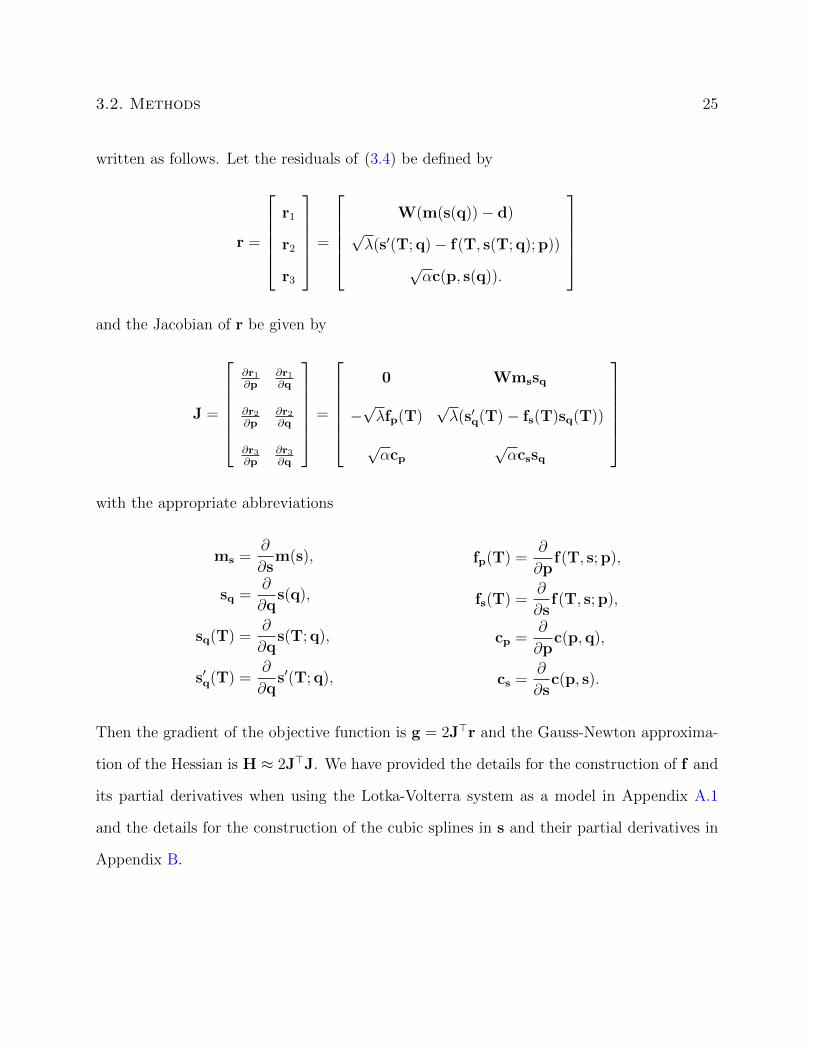
3.2. Methods 25
written as follows. Let the residuals of (3.4) be defined by
r =
r1
r2
r3
=
W(m(s(q))− d)
√λ(s′(T; q)− f(T, s(T; q); p))
√αc(p, s(q)).
and the Jacobian of r be given by
J =
∂r1∂p
∂r1∂q
∂r2∂p
∂r2∂q
∂r3∂p
∂r3∂q
=
0 Wmssq
−√λfp(T)
√λ(s′q(T)− fs(T)sq(T))
√αcp
√αcssq
with the appropriate abbreviations
ms =∂
∂sm(s),
sq =∂
∂qs(q),
sq(T) =∂
∂qs(T; q),
s′q(T) =∂
∂qs′(T; q),
fp(T) =∂
∂pf(T, s; p),
fs(T) =∂
∂sf(T, s; p),
cp =∂
∂pc(p,q),
cs =∂
∂sc(p, s).
Then the gradient of the objective function is g = 2J>r and the Gauss-Newton approxima-
tion of the Hessian is H ≈ 2J>J. We have provided the details for the construction of f and
its partial derivatives when using the Lotka-Volterra system as a model in Appendix A.1
and the details for the construction of the cubic splines in s and their partial derivatives in
Appendix B.
26 Chapter 3. Parameter Estimation for Microbiota Models
3.3 Results and Discussion
In this section we apply principal differential analysis to biological systems using simulation
studies and previously collected and published data for both intestinal and vaginal microbiota
and share our findings. We focused on the Lotka-Volterra system of differential equations as a
model and included an unknown sparsity pattern in the interaction matrix as an assumption
and constraint on the model.
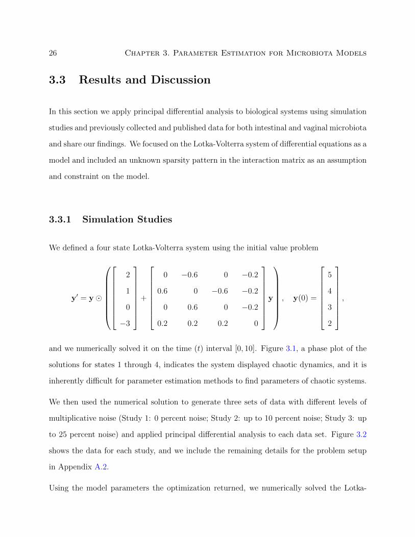
3.3.1 Simulation Studies
We defined a four state Lotka-Volterra system using the initial value problem
y′ = y �
2
1
0
−3
+
0 −0.6 0 −0.2
0.6 0 −0.6 −0.2
0 0.6 0 −0.2
0.2 0.2 0.2 0
y
, y(0) =
5
4
3
2
,
and we numerically solved it on the time (t) interval [0, 10]. Figure 3.1, a phase plot of the
solutions for states 1 through 4, indicates the system displayed chaotic dynamics, and it is
inherently difficult for parameter estimation methods to find parameters of chaotic systems.
We then used the numerical solution to generate three sets of data with different levels of
multiplicative noise (Study 1: 0 percent noise; Study 2: up to 10 percent noise; Study 3: up
to 25 percent noise) and applied principal differential analysis to each data set. Figure 3.2
shows the data for each study, and we include the remaining details for the problem setup
in Appendix A.2.
Using the model parameters the optimization returned, we numerically solved the Lotka-

3.3. Results and Discussion 27
Figure 3.1: Numerical solution of a Lotka-Volterra system from t = 0 to t = 200.
0 2 4 6 8 100
5
10
15
20State 1
0 2 4 6 8 100
1
2
3
4
5State 2
0 2 4 6 8 10Time
0
5
10
15State 3
0 2 4 6 8 10Time
0
5
10
15
20State 4
Figure 3.2: Simulated data points from the numerical solution of a Lotka-Volterra system.Black: Numerical solution. Blue: Data with no multiplicative noise. Red: Data with up to10 percent multiplicative noise. Yellow: Data with up to 25 percent multiplicative noise.
Volterra system and compared the solution to the data. The relative errors er = ‖m(y)−d‖2‖d‖2
were approximately er ≈ 0.0258, er ≈ 0.0794, and er ≈ 0.1314 for studies 1, 2, and 3,
respectively, so principal differential analysis was able to recover the data.
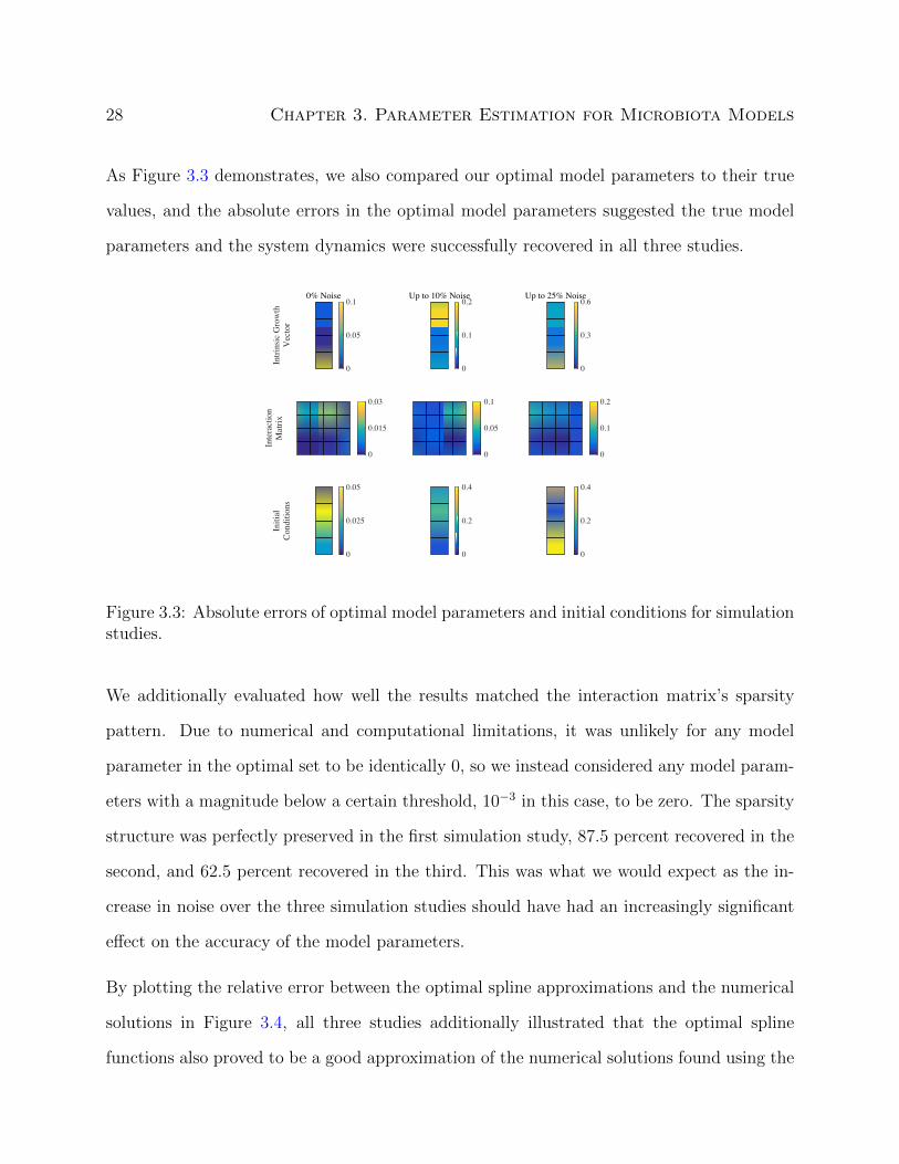
28 Chapter 3. Parameter Estimation for Microbiota Models
As Figure 3.3 demonstrates, we also compared our optimal model parameters to their true
values, and the absolute errors in the optimal model parameters suggested the true model
parameters and the system dynamics were successfully recovered in all three studies.
0% Noise
Intri
nsic
Gro
wth
Vec
tor
0
0.05
0.1
Inte
ract
ion
Mat
rix
0
0.015
0.03
Initi
alCo
nditi
ons
0
0.025
0.05
Up to 10% Noise
0
0.1
0.2
0
0.05
0.1
0
0.2
0.4
Up to 25% Noise
0
0.3
0.6
0
0.1
0.2
0
0.2
0.4
Figure 3.3: Absolute errors of optimal model parameters and initial conditions for simulationstudies.
We additionally evaluated how well the results matched the interaction matrix’s sparsity
pattern. Due to numerical and computational limitations, it was unlikely for any model
parameter in the optimal set to be identically 0, so we instead considered any model param-
eters with a magnitude below a certain threshold, 10−3 in this case, to be zero. The sparsity
structure was perfectly preserved in the first simulation study, 87.5 percent recovered in the
second, and 62.5 percent recovered in the third. This was what we would expect as the in-
crease in noise over the three simulation studies should have had an increasingly significant
effect on the accuracy of the model parameters.
By plotting the relative error between the optimal spline approximations and the numerical
solutions in Figure 3.4, all three studies additionally illustrated that the optimal spline
functions also proved to be a good approximation of the numerical solutions found using the
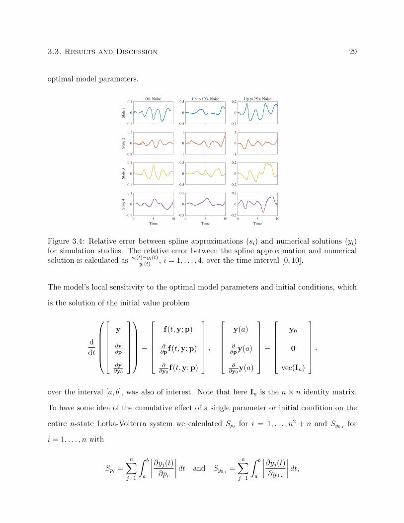
3.3. Results and Discussion 29
optimal model parameters.
-0.1
0
0.1
Stat
e 1
0% Noise
-0.5
0
0.5
Stat
e 2
-0.1
0
0.1
Stat
e 3
0 5 10Time
-0.1
0
0.1
Stat
e 4
-0.5
0
0.5Up to 10% Noise
-1
0
1
-0.5
0
0.5
0 5 10Time
-0.5
0
0.5
-0.2
0
0.2Up to 25% Noise
-1
0
1
-0.2
0
0.2
0 5 10Time
-0.2
0
0.2
Figure 3.4: Relative error between spline approximations (si) and numerical solutions (yi)for simulation studies. The relative error between the spline approximation and numericalsolution is calculated as si(t)−yi(t)
yi(t), i = 1, . . . , 4, over the time interval [0, 10].
The model’s local sensitivity to the optimal model parameters and initial conditions, which
is the solution of the initial value problem
d
dt
y
∂y∂p
∂y∂y0
=
f(t,y; p)
∂∂p
f(t,y; p)
∂∂y0
f(t,y; p)
,
y(a)
∂∂p
y(a)
∂∂y0
y(a)
=
y0
0
vec(In)
,
over the interval [a, b], was also of interest. Note that here In is the n × n identity matrix.
To have some idea of the cumulative effect of a single parameter or initial condition on the
entire n-state Lotka-Volterra system we calculated Spi for i = 1, . . . , n2 + n and Sy0,i for
i = 1, . . . , n with
Spi =n∑j=1
∫ b
a
∣∣∣∣∂yj(t)∂pi
∣∣∣∣ dt and Sy0,i =n∑j=1
∫ b
a
∣∣∣∣∂yj(t)∂y0,i
∣∣∣∣ dt,
30 Chapter 3. Parameter Estimation for Microbiota Models
respectively, and provide the results in Figure 3.5.
0% Noise
Intri
nsic
Gro
wth
Vec
tor
0
150
300
Inte
ract
ion
Mat
rix
0
1500
3000
Initi
alCo
nditi
ons
0
25
50
Up to 10% Noise
0
200
400
0
2000
4000
0
30
60
Up to 25% Noise
0
150
300
0
1500
3000
0
25
50
Figure 3.5: Cumulative local sensitivities of optimal model parameters and initial conditionsfor simulation studies.
The cumulative sensitivities remained consistent across the three simulation studies, which
was not surprising given the consistency across the simulation studies in the optimal model
parameters and initial conditions themselves.
3.3.2 Intestinal Microbiota Dynamics
The generalized Lotka-Volterra formalism was recently used to explore the impact of the in-
testinal microbiota on the development of antibiotic-induced Clostridium difficile colitis [71].
This disease occurs in patients who have been treated with antibiotics and is characterized
by a marked shift of the intestinal microbiota towards a state dominated by the pathogen
Clostridium difficile. In many cases health can only be restored through a fecal transplant,
a procedure which restores the diversity of the microbiota. The mechanisms through which
disease occurs and through which the normal gut microbiota can prevent the over-growth of
C. difficile are still not well understood.

3.3. Results and Discussion 31
In Stein et al. [71] the authors relied on a mouse model of C. difficile colitis to attempt
to address these questions. They tracked the microbiota of mice across time and used the
resulting data to estimate the parameters of a Lotka-Volterra model. Based on the resulting
model they were able to provide new testable hypotheses about the factors that promote
the overgrowth of C. difficile following a course of clindamycin. Here we used the same
data and model and added the assumption of sparsity in the interaction matrix. We applied
principal differential analysis and compared the outcome to the originally published results.
We focused on a subset of the Stein et al. data, specifically data originating from three mice
who had not been subjected to any antibiotic interventions. The exact details including how
we set up our problem can be found in the Appendix A.3.
In our simulation, the optimal spline approximations remained good approximations to the
numerical solutions using the optimal model parameters as demonstrated in Figure 3.6.
The relative errors for the spline approximations for the Blautia and Coprobacillus OTUs
were larger than the relative errors for the other five OTUs, but this was due to both the
significantly smaller magnitude of the data for these OTUs and the magnitude of the weights
for the data relative to the other OTUs. Among the three replicates for a single OTU,
variations in the magnitude of the relative errors, e.g., in Blautia, Unclassified Mollicutes,
and Coprobacillus, were explained by noticeable variations in the magnitude of the data
across replicates.
As in the simulation studies, we also evaluated the data recovery. The relative error between
the numerical solutions using the optimal model parameters and the data for all three mice
given by er = ‖m(y)−d‖2‖d‖2 was er ≈ 0.3027. The relative error for the model published in [71]
was er ≈ 0.5127, which indicates that our method more accurately captured the dynamics of
the data. This fact was further confirmed by a visual comparison of the numerical solutions
to the data in Figure 3.7.

32 Chapter 3. Parameter Estimation for Microbiota Models
-1000
100Replicate 1
Blautia
-0.050
0.05
Barnesiella
-505
UnclassifiedMollicutes
-0.10
0.1Undefined
Lachnospiraceae
-0.020
0.02Unclassified
Lachnospiraceae
-101
Coprobacillus
0 10 20Time
-0.020
0.02
Other
-202
Replicate 2
-0.020
0.02
-0.50
0.5
-0.050
0.05
-0.020
0.02
-100
10
0 10 20Time
-0.020
0.02
-202
Replicate 3
-0.020
0.02
-0.50
0.5
-0.050
0.05
-0.020
0.02
-200
20
0 10 20Time
-0.010
0.01
Figure 3.6: Relative error between spline approximations (si) and numerical solutions (yi)for intestinal microbiota model. The relative error between the spline approximation andnumerical solution is calculated as si(t)−yi(t)
yi(t), i = 1, . . . , 7, over the time interval [1, 21]. Time
is measured in days.
00.10.2
Replicate 1
Blautia
05
10
Barnesiella
0
0.5UnclassifiedMollicutes
024
UndefinedLachnospiraceae
012
UnclassifiedLachnospiraceae
00.020.04
Coprobacillus
0 10 20Time
012
Other
00.10.2
Replicate 2
123
00.20.4
0
5
00.5
1
00.0050.01
0 10 20Time
123
00.20.4
Replicate 3
05
10
00.20.4
05
10
012
00.010.02
0 10 20Time
0
5
Figure 3.7: Comparison of numerical solutions for intestinal microbiota model. Black: Ex-perimental data. Blue: Numerical solutions based on optimal Lotka-Volterra system fromprincipal differential analysis. Red: Numerical solutions found using the optimal Lotka-Volterra system published in [71]. Time is measured in days, and abundance is measured in1011 DNA copies per cubic centimeter.
3.3. Results and Discussion 33
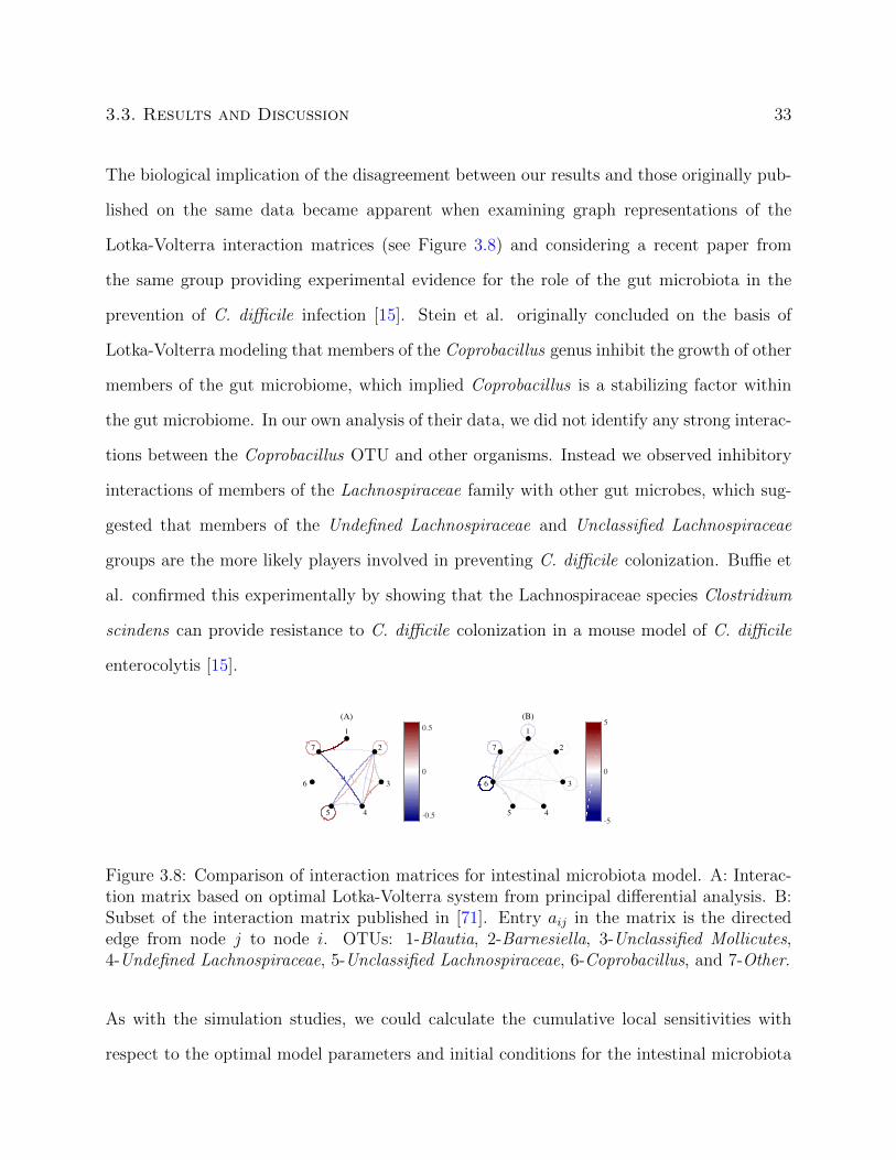
The biological implication of the disagreement between our results and those originally pub-
lished on the same data became apparent when examining graph representations of the
Lotka-Volterra interaction matrices (see Figure 3.8) and considering a recent paper from
the same group providing experimental evidence for the role of the gut microbiota in the
prevention of C. difficile infection [15]. Stein et al. originally concluded on the basis of
Lotka-Volterra modeling that members of the Coprobacillus genus inhibit the growth of other
members of the gut microbiome, which implied Coprobacillus is a stabilizing factor within
the gut microbiome. In our own analysis of their data, we did not identify any strong interac-
tions between the Coprobacillus OTU and other organisms. Instead we observed inhibitory
interactions of members of the Lachnospiraceae family with other gut microbes, which sug-
gested that members of the Undefined Lachnospiraceae and Unclassified Lachnospiraceae
groups are the more likely players involved in preventing C. difficile colonization. Buffie et
al. confirmed this experimentally by showing that the Lachnospiraceae species Clostridium
scindens can provide resistance to C. difficile colonization in a mouse model of C. difficile
enterocolytis [15].
(A)1
2
3
45
6
7
-0.5
0
0.5(B)1
2
3
45
6
7
-5
0
5
Figure 3.8: Comparison of interaction matrices for intestinal microbiota model. A: Interac-tion matrix based on optimal Lotka-Volterra system from principal differential analysis. B:Subset of the interaction matrix published in [71]. Entry aij in the matrix is the directededge from node j to node i. OTUs: 1-Blautia, 2-Barnesiella, 3-Unclassified Mollicutes,4-Undefined Lachnospiraceae, 5-Unclassified Lachnospiraceae, 6-Coprobacillus, and 7-Other.
As with the simulation studies, we could calculate the cumulative local sensitivities with
respect to the optimal model parameters and initial conditions for the intestinal microbiota

34 Chapter 3. Parameter Estimation for Microbiota Models
model. Note that because of how the parameter estimation problem was set up (see Ap-
pendix A.3), the resulting model parameters for each of the three replicates were the same,
but the optimal initial conditions differed. This meant the local sensitivities and hence
the cumulative sensitivities could vary by replicate, yet the results in Figure 3.9 display
consistency in the cumulative sensitivities across the replicates.
Replicate 1
Intri
nsic
Gro
wth
Vec
tors
0
250
500
Inte
ract
ion
Mat
rices
0
500
1000
Initi
alCo
nditi
ons
0
80
160
Replicate 2
0
250
500
0
500
1000
0
40
80
Replicate 3
0
250
500
0
600
1200
0
40
80
Figure 3.9: Cumulative local sensitivities of optimal model parameters and initial conditionsfor intestinal microbiota model.
3.3.3 Vaginal Microbiota Dynamics
Gajer et al. described the temporal dynamics of the human vaginal microbiome sampled
twice per week over a 16-week period in 32 women [29]. Understanding the factors that
drive community structure in this environment may provide insights into the stability of the
system and the disruptions that lead to the development of bacterial vaginosis, a condition
impacting millions of women in the United States. These data are more deeply sampled than
the Stein et al. data set described above, which leads to a clearer picture of the system’s
dynamics.
3.3. Results and Discussion 35
We present here the results of analyzing the data obtained from subject 15 in the original
study. We chose this particular subject because the data for this subject included most of
the OTUs we determined are likely to play important role in the dynamics of the vaginal
microbiota. We include the details of the analysis used to select this subject in Appendix A.4.
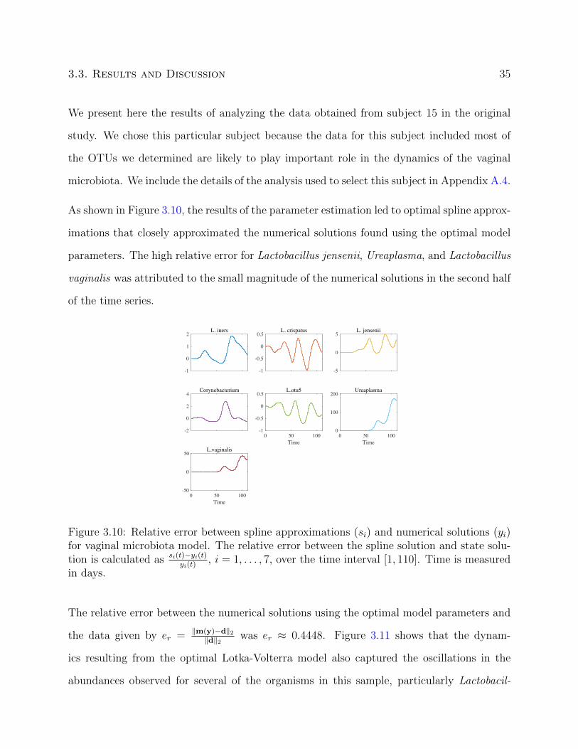
As shown in Figure 3.10, the results of the parameter estimation led to optimal spline approx-
imations that closely approximated the numerical solutions found using the optimal model
parameters. The high relative error for Lactobacillus jensenii, Ureaplasma, and Lactobacillus
vaginalis was attributed to the small magnitude of the numerical solutions in the second half
of the time series.
-1
0
1
2L. iners
-1
-0.5
0
0.5L. crispatus
-5
0
5L. jensenii
-2
0
2
4Corynebacterium
0 50 100Time
-1
-0.5
0
0.5L.otu5
0 50 100Time
0
100
200Ureaplasma
0 50 100Time
-50
0
50L.vaginalis
Figure 3.10: Relative error between spline approximations (si) and numerical solutions (yi)for vaginal microbiota model. The relative error between the spline solution and state solu-tion is calculated as si(t)−yi(t)
yi(t), i = 1, . . . , 7, over the time interval [1, 110]. Time is measured
in days.
The relative error between the numerical solutions using the optimal model parameters and
the data given by er = ‖m(y)−d‖2‖d‖2 was er ≈ 0.4448. Figure 3.11 shows that the dynam-
ics resulting from the optimal Lotka-Volterra model also captured the oscillations in the
abundances observed for several of the organisms in this sample, particularly Lactobacil-

36 Chapter 3. Parameter Estimation for Microbiota Models
lus crispatus and Lactobacillus otu5. This result was surprising given that the oscillations
are at least in part due to the physiological changes that occur during menstrual periods.
The dynamics that the optimal Lotka-Volterra model captured indicate that inter-microbe
interactions may play a role in these periodic changes as well.
0
5000
10000L. iners
0
5
10L. crispatus
0
1000
2000L. jensenii
0
20
40
60Corynebacterium
0 50 100Time
0
50
100L.otu5
0 50 100Time
0
50
100Ureaplasma
0 50 100Time
0
5
10
15L.vaginalis
Figure 3.11: Comparison of numerical solutions to data for vaginal microbiota model. Col-ored Curve: Numerical solution. Black Dots: Experimental data. Time is measured in days,and the abundance is the number of 16S rRNA gene sequence reads.
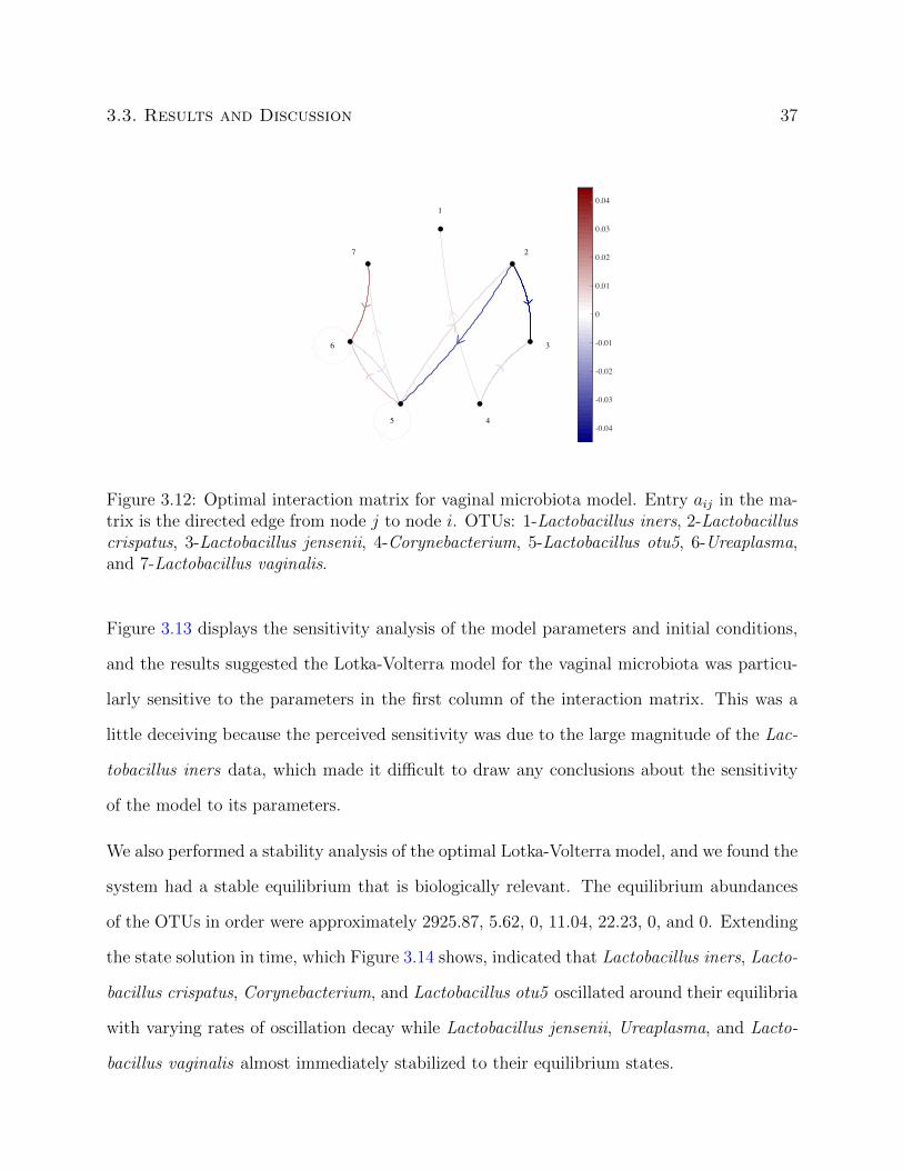
The graph of the interaction matrix displayed in Figure 3.12 also highlights that the dynamics
of the optimal Lotka-Volterra model were due in part to several particular interactions. The
OTU Lactobacillus crispatus had strong negative interactions with Lactobacillus jensenii and
Lactobacillus otu5, indicating a possible role for this organism in maintaining the stability
of the vaginal microbiota. This observation was in agreement with previously reported
epidemiological observations [83] that suggest Lactobacillus crispatus is a stabilizing factor
in the human vaginal microbiota. The OTU Lactobacillus otu5 also had positive interactions
with multiple members of the vaginal microbiota suggesting this organism may produce
compounds necessary for their growth and providing an initial insight into the potential
function of this uncharacterized OTU.
3.3. Results and Discussion 37
1
2
3
45
6
7
-0.04
-0.03
-0.02
-0.01
0
0.01
0.02
0.03
0.04
Figure 3.12: Optimal interaction matrix for vaginal microbiota model. Entry aij in the ma-trix is the directed edge from node j to node i. OTUs: 1-Lactobacillus iners, 2-Lactobacilluscrispatus, 3-Lactobacillus jensenii, 4-Corynebacterium, 5-Lactobacillus otu5, 6-Ureaplasma,and 7-Lactobacillus vaginalis.
Figure 3.13 displays the sensitivity analysis of the model parameters and initial conditions,
and the results suggested the Lotka-Volterra model for the vaginal microbiota was particu-
larly sensitive to the parameters in the first column of the interaction matrix. This was a
little deceiving because the perceived sensitivity was due to the large magnitude of the Lac-
tobacillus iners data, which made it difficult to draw any conclusions about the sensitivity
of the model to its parameters.
We also performed a stability analysis of the optimal Lotka-Volterra model, and we found the
system had a stable equilibrium that is biologically relevant. The equilibrium abundances
of the OTUs in order were approximately 2925.87, 5.62, 0, 11.04, 22.23, 0, and 0. Extending
the state solution in time, which Figure 3.14 shows, indicated that Lactobacillus iners, Lacto-
bacillus crispatus, Corynebacterium, and Lactobacillus otu5 oscillated around their equilibria
with varying rates of oscillation decay while Lactobacillus jensenii, Ureaplasma, and Lacto-
bacillus vaginalis almost immediately stabilized to their equilibrium states.
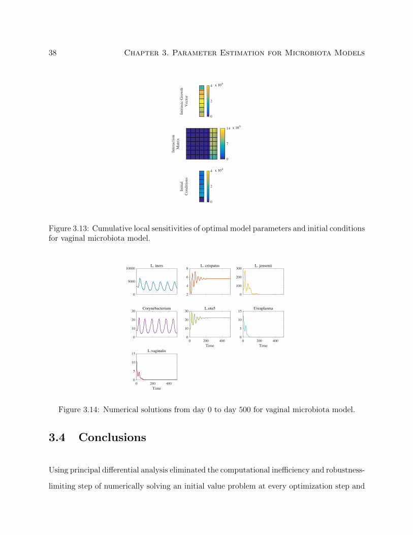
38 Chapter 3. Parameter Estimation for Microbiota Models
x 106
Intri
nsic
Gro
wth
Vec
tor
0
2
4
x 109
Inte
ract
ion
Mat
rix
0
7
14
x 104
Initi
alCo
nditi
ons
0
2
4
Figure 3.13: Cumulative local sensitivities of optimal model parameters and initial conditionsfor vaginal microbiota model.
0
5000
10000L. iners
2
4
6
8L. crispatus
0
100
200
300L. jensenii
0
10
20
30Corynebacterium
0 200 400Time
0
10
20
30L.otu5
0 200 400Time
0
5
10
15Ureaplasma
0 200 400Time
0
5
10
15L.vaginalis
Figure 3.14: Numerical solutions from day 0 to day 500 for vaginal microbiota model.
3.4 Conclusions
Using principal differential analysis eliminated the computational inefficiency and robustness-
limiting step of numerically solving an initial value problem at every optimization step and
3.4. Conclusions 39
also presents a natural framework for including prior knowledge or assumptions about the
biological system being modeled. In defining and solving this new problem, we demonstrated
that we did not sacrificed parameter or data recovery. This suggested this approach is
a valuable tool, particularly for increasingly complex parameter estimation problems like
those found in systems biology.
Biologically speaking, principal differential analysis demonstrated the ability to closely model
real biological data. In the case of the vaginal microbiota, the approach was able to cap-
ture the general abundance dynamics seen in the data and provide a full forward projection
for the system. We would like to note though that the resulting model did not provide a
full forward prediction in the case of the intestinal microbiota. The Lotka-Volterra system
appeared to be unstable leading to the uncontrolled growth or the disappearance of certain
taxa, phenomena not commonly observed in real data. In part this was due to the limitations
of the Lotka-Volterra system and the simplifying assumptions made when choosing it as a
model. Insufficient data both in terms of the relatively small number of samples and, more
importantly, in terms of the sparse sampling rate also played a role. Unfortunately, these
limitations are inherent as computational costs can require model simplifications, experi-
mental costs can limit the number of feasibly obtained samples, and the specific microbiome
being sampled can potentially limit the sampling frequency.
Despite these limitations, we showed that we could identify interactions and their direction
between members of the intestinal microbiome that were later confirmed by in vivo experi-
ments. The approach we described here correctly identified the experimentally validated role
of the Lachnospiraceae family as a stabilizing factor in the intestinal microbiome in contrast
with the suggestion that the Coprobacillus OTU plays this role as predicted by a previous
computational analysis. Likewise, our analysis correctly identified the role of Lactobacillus
crispatus as an important contributor to the stability of the vaginal microbiome. The net-

40 Chapter 3. Parameter Estimation for Microbiota Models
work we inferred also provided insights into the roles played by uncharacterized members of
the vaginal community such as the organisms known as Lactobacillus otu5. Knowledge of
the underlying interactions and their direction like these are an important aspect of guiding
further biological experimentation.
Modeling approaches that exhibit robustness while having an appropriate theoretical frame-
work are extremely useful in understanding host-associated microbial communities. The
examples we provided here demonstrate how much information we can gather from experi-
mental data when paired with the right inference approach, and we believe that approaches
like principal differential analysis when paired with experimental work can help elucidate
the role of host-associated microbes in health and disease.
Chapter 4
Least-Squares Finite Element Method
4.1 Introduction
Perhaps one reason parameter estimation methods like principal differential analysis are
underutilized is the relative popularity and maturity of finite difference methods for solving
ordinary differential equations [13]. There exists well-developed theory including conditions
for the stability and convergence of finite difference methods, and we have methods optimized
for specific types of differential equations like stiff or non-stiff equations [2, 13]. On the
other hand, finite element methods first emerged in the 1950s and their initial development
focused on solving partial differential equations [41]. As a result the now established theory
for finite element methods predominantly relates to partial differential equations as do most
applications. Thus, it makes sense that many traditional parameter estimation methods,
like shooting methods, are built on finite difference methods.
In more recent years however much work has been done to extend finite element methods to
ordinary differential equations, and while we do not claim a comprehensive list of published
41

42 Chapter 4. Least-Squares Finite Element Method
work, much of the focus has been on extending Galerkin finite element methods [1, 9, 13].
We however cannot guarantee these methods are unconditionally stable [75], so we must
either adapt the Galerkin methods or find an alternative approach.
Least-squares finite element methods are an example of such an alternative, and while they
are stable for all ordinary differential equations [75], the methods have other advantages. Un-
like Galerkin methods, least-squares methods have universal application and do not require
modification for particular problems [40]. This makes the methods both robust and easy
to implement for repeated, diverse use [10, 40], which validates the usefulness of parameter
estimation methods like principal differential analysis that are built on them.
Readers can refer to [10, 40] for additional details on the least-squares finite element method,
so what follows is a detailed discussion of our approach for initial value problems. We
also include multiple examples to touch on some of the points above and to highlight the
advantages of least-squares methods. We should also note that the derivation for boundary
value problems is essentially identical to what follows, so we focus on initial value problems
and highlight the one difference for boundary value problems via example in Section 4.3.2.
4.2 Methods
4.2.1 Problem Statement
Given the initial value problem
y′ = f(t,y), y(a) = y0,
4.2. Methods 43
we assume the conditions for Theorem 2.1 are satisfied. Finding the unique solution of the
initial value problem means finding a function y such that y satisfies the differential equation
y′ = f(t,y) for some interval [a, b] and the initial conditions y(a) = y0 [54].
Given the continuity requirement on y, we can rewrite this objective as
miny‖y′ − f(t,y)‖pLp
subject to y(a) = y0,
where ‖ · ‖Lp is any appropriate integral norm on the interval [a, b] with p = 2 for the
remainder of this chapter. Note that the minimum of this objective is necessarily zero since
we know a unique solution exists.
We replace y with an approximating function s that we can uniquely define by a set of
parameters q to create the new objective
minq‖s′(q)− f(t, s(q))‖2L2
subject to s(a) = y0.
(4.1)
Depending on the unique solution y and the choice of approximating function s, it is possible
that s = y, but this is not true in general, which means we can no longer guarantee zero
is the minimum value of the objective. This means we are no longer solving the original
problem, but as we explain in Section 3.2.5 for the parameter estimation problem, we are
solving a “nearby” one.
The last step of the derivation is to choose an approximation for the L2-norm to arrive at
the objective
minq‖W(s′(T; q)− f(T, s(T; q)))‖22
subject to s(t0) = y0,
(4.2)
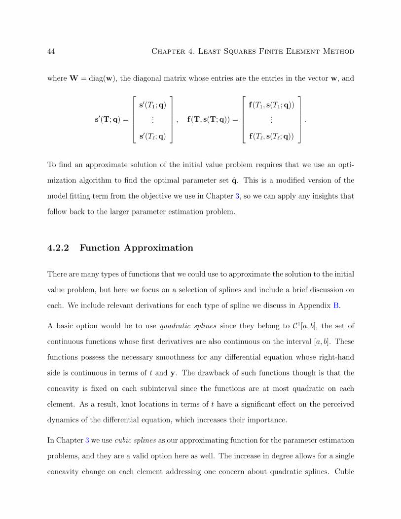
44 Chapter 4. Least-Squares Finite Element Method
where W = diag(w), the diagonal matrix whose entries are the entries in the vector w, and
s′(T; q) =
s′(T1; q)
...
s′(T`; q)
, f(T, s(T; q)) =
f(T1, s(T1; q))
...
f(T`, s(T`; q))
.
To find an approximate solution of the initial value problem requires that we use an opti-
mization algorithm to find the optimal parameter set q. This is a modified version of the
model fitting term from the objective we use in Chapter 3, so we can apply any insights that
follow back to the larger parameter estimation problem.
4.2.2 Function Approximation
There are many types of functions that we could use to approximate the solution to the initial
value problem, but here we focus on a selection of splines and include a brief discussion on
each. We include relevant derivations for each type of spline we discuss in Appendix B.
A basic option would be to use quadratic splines since they belong to C1[a, b], the set of
continuous functions whose first derivatives are also continuous on the interval [a, b]. These
functions possess the necessary smoothness for any differential equation whose right-hand
side is continuous in terms of t and y. The drawback of such functions though is that the
concavity is fixed on each subinterval since the functions are at most quadratic on each
element. As a result, knot locations in terms of t have a significant effect on the perceived
dynamics of the differential equation, which increases their importance.
In Chapter 3 we use cubic splines as our approximating function for the parameter estimation
problems, and they are a valid option here as well. The increase in degree allows for a single
concavity change on each element addressing one concern about quadratic splines. Cubic
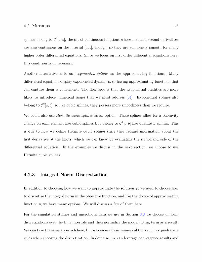
4.2. Methods 45
splines belong to C2[a, b], the set of continuous functions whose first and second derivatives
are also continuous on the interval [a, b], though, so they are sufficiently smooth for many
higher order differential equations. Since we focus on first order differential equations here,
this condition is unnecessary.
Another alternative is to use exponential splines as the approximating functions. Many
differential equations display exponential dynamics, so having approximating functions that
can capture them is convenient. The downside is that the exponential qualities are more
likely to introduce numerical issues that we must address [64]. Exponential splines also
belong to C2[a, b], so like cubic splines, they possess more smoothness than we require.
We could also use Hermite cubic splines as an option. These splines allow for a concavity
change on each element like cubic splines but belong to C1[a, b] like quadratic splines. This
is due to how we define Hermite cubic splines since they require information about the
first derivative at the knots, which we can know by evaluating the right-hand side of the
differential equation. In the examples we discuss in the next section, we choose to use
Hermite cubic splines.
4.2.3 Integral Norm Discretization
In addition to choosing how we want to approximate the solution y, we need to choose how
to discretize the integral norm in the objective function, and like the choice of approximating
function s, we have many options. We will discuss a few of them here.
For the simulation studies and microbiota data we use in Section 3.3 we choose uniform
discretizations over the time intervals and then normalize the model fitting term as a result.
We can take the same approach here, but we can use basic numerical tools such as quadrature
rules when choosing the discretization. In doing so, we can leverage convergence results and

46 Chapter 4. Least-Squares Finite Element Method
related theory, which have been well-established in literature.
One option is using an n-point Gauss-Legendre quadrature, which is exact for polynomials
up to degree 2n− 1 [74]. If the approximating function we choose is a polynomial spline, for
example, and the right-hand side of the differential equation is polynomial in terms of t and
y, then the integrand in (4.1) is a polynomial on each element as well. This means that if
we construct the vector of evaluation points T and the corresponding weight matrix W by
applying the quadrature rule on each element, then (4.2) is equivalent to (4.1) as long as n
is sufficiently large.
Another quadrature option that we can leverage in the same way is an n-point Gauss-
Lobatto quadrature, which is exact for polynomials up to degree 2n − 3 [74]. This might
seem unnecessary since a Gauss-Legendre quadrature requires one less quadrature point
for the same accuracy, but this is not always the case. When paired with Hermite cubic
splines as the approximating functions, we only require n−2 evaluation points of an n-point
Gauss-Lobatto quadrature rule. This is because two of the evaluation points for the Gauss-
Lobatto quadrature are the endpoints of the interval, and in this case the endpoints are the
spline knots for each element. Since the Hermite cubic splines use the right-hand side of
the differential equation for information about the first derivative, the spline satisfies the
differential equation exactly at the knots, which means these evaluation points contribute
nothing to the objective, so we can ignore the endpoints for the Gauss-Lobatto quadrature.
We use this approach in the examples that follow in the next section.
4.2.4 Adaptive Schemes
When choosing splines as approximating functions, we must also decide on the number of
knots we would like to use for the interval of interest. We could choose a fixed number, but

4.3. Results and Discussion 47
this can lead to poor results. If we choose too few knots, the approximate solution might
include significant error, but if we choose too many knots, finding the approximate solution
could become computationally onerous. As a result, we could benefit from an approach that
allows us to adapt the number and location of knots.
One such approach when using a quadrature rule for the discretization of the integral norm is
to use the residuals in (4.2) to determine where we should place new knots. Given an initial
selection of knots, we can solve (4.2) and then identify the element that contributes the most
to the objective function. We can then place a new knot in the middle of the element and
solve (4.2) again repeating this process until the residuals for all of the elements fall below
a predetermined threshold.
There are also simple variations of this approach such as placing multiple new knots in the
element that contributes the most to the objective function or placing a new knot in each of
the k elements that contribute most to the objective function or some combination thereof.
For simplicity the adaptive scheme we use for the example in Section 4.3.4 is placing a single
knot in the middle of the element that contributes the most to the objective function.
4.3 Results and Discussion
In this section we apply the least-squares finite element method to a selection of example
ordinary differential equations. We focus on examples that demonstrate the robustness,
competitiveness, and versatility of the least-squares method when compared to standard
finite difference methods (initial value problems) and collocation methods (boundary value
problems).

48 Chapter 4. Least-Squares Finite Element Method
4.3.1 Linear Initial Value Problem
We considered the initial value problem
y′ = y − 2e−t, y(0) = 1,
which has a solution of y(t) = e−t. We used a Hermite cubic spline with 31 knots uniformly
distributed over the t-interval [0, 30] and chose a five-point Gauss-Lobatto quadrature for
the evaluation points on each element. Solving the initial value problem using MATLAB’s
ode45 and the least-squares method led to the following results.
0 5 10 15 20 25 30
0
0.2
0.4
0.6
0.8
1State
0 5 10 15 20 25 30t
-2
-1
0
1
2 ×10⁻³ State Error
Figure 4.1: Solutions of linear initial value problem. Blue: Analytic solution. Purple: ode45solution. Red: Least-squares solution with dots indicating knot placement.
Figure 4.1 indicates that the error in the ode45 solution grew to an unreasonable level over
the course of the interval, but the FEM solution had a maximum error on the order of 10−3.
Using a stiff solver like MATLAB’s ode23s resulted in the same outcome with the error
growing to an even larger magnitude than it did with ode45.

4.3. Results and Discussion 49
4.3.2 Two State Linear Initial Value Problem
We considered the linear system
y′ =
0 1
µ2 0
y +
0
(µ2 + p2) sin(pt)
, y(0) =
0
p
,where µ = 60 and p = π. The solution of this initial value problem is
y =
sin(πt)
π cos(πt)
.For both states we used Hermite cubic splines with 11 knots uniformly distributed over the
t-interval [0, 1]. We again chose a five-point Gauss-Lobatto quadrature for the evaluation
points on each element, and Figure 4.2 shows the solutions using ode45 and the least-squares
method.
0 0.2 0.4 0.6 0.8 10
0.2
0.4
0.6
0.8
1
Stat
e 1
State
0 0.2 0.4 0.6 0.8 1-2
-1
0
1
2 ×10⁻⁵ State Error
0 0.2 0.4 0.6 0.8 1t
-4
-2
0
2
4
Stat
e 2
0 0.2 0.4 0.6 0.8 1t
-1
-0.5
0
0.5
1 ×10⁻³
Figure 4.2: Solutions of two state linear initial value problem. Blue: Analytic solution.Purple: ode45 solution. Red: Least-squares solution with dots indicating knot placement.

50 Chapter 4. Least-Squares Finite Element Method
The ode45 solution began to deviate from the analytic solution almost immediately while
the least-squares solution had a maximum error on the order of 10−3. As in the previous
example using ode23s did not change the outcome, and the maximum error was worse than
the error using ode45.
We can also view this example in the context of a parameter estimation problem where π
is the true value of the unknown parameter p. This example demonstrates that when the
unknown parameter was set to its true value, standard finite difference methods failed to
solve the initial value problem making the estimation of the unknown parameter impossible.
This supports the significance of the work we shared in Chapter 3.
We also rewrote this example as a boundary value problem by replacing the initial conditions
with the boundary conditions y1(0) = 0, y2(1) = −p, so the solution is unchanged. We again
used Hermite cubic splines but with 21 knots uniformly distributed over the t-interval [0, 1]
for both states and chose a five-point Gauss-Lobatto quadrature for the evaluation points
on each element. Solving the boundary value problem with MATLAB’s bvp4c and the
least-squares method gave the results shown in Figure 4.3.
The errors for both the bvp4c solution and the least-squares solution were almost identical
for state 1 and on the same order for state 2, but the bvp4c solution required roughly twice
the computational time as the least-squares method (0.0066 seconds versus 0.0032 seconds).
Note that changing the problem from an initial value problem to a boundary value problem
required that we use a completely different MATLAB function to solve the problem, but
the least-squares method was exactly the same other than the pre-computational step of
identifying which knots to view as fixed. This highlights the versatility of the FEM approach.
4.3. Results and Discussion 51
0 0.2 0.4 0.6 0.8 1-0.5
0
0.5
1
1.5
Stat
e 1
State
0 0.2 0.4 0.6 0.8 1-1
-0.5
0
0.5
1
1.5 ×10⁻⁶ State Error
0 0.2 0.4 0.6 0.8 1t
-4
-2
0
2
4
Stat
e 2
0 0.2 0.4 0.6 0.8 1t
-3
-2
-1
0
1
2
3 ×10⁻⁵
Figure 4.3: Solutions of two state linear boundary value problem. Blue: Analytic solution.Purple: bvp4c solution. Red: Least-squares solution with dots indicating knot placement.
4.3.3 Nonlinear Initial Value Problem
We also worked with a nonlinear, ordinary differential equation by considering the initial
value problem
y′ = y − y2, y(0) =1
2,
which has a solution of y(t) = 11+e−t . We used a Hermite cubic spline with 21 knots uniformly
distributed over the t-interval [0, 10] and chose an eight-point Gauss-Lobatto quadrature as
the evaluation points on each element for the least-squares method. Solving the initial value
problem with this setup and also with ode45 gave the results displayed in Figure 4.4.
The least-squares solution had a smaller maximum error than the ode45 solution, but the
accuracy came at the expense of computational time as ode45 required roughly a fourth of
the computational time (0.0015 seconds versus 0.0055 seconds). The point though was to
show that the least-squares method does not require the differential equation to be linear.

52 Chapter 4. Least-Squares Finite Element Method
0 1 2 3 4 5 6 7 8 9 100.5
0.6
0.7
0.8
0.9
1State
0 1 2 3 4 5 6 7 8 9 10t
-2
0
2
4
6 ×10⁻⁵ State Error
Figure 4.4: Solutions of nonlinear initial value problem. Blue: Analytic solution. Purple:ode45 solution. Red: Least-squares solution with dots indicating knot placement.
4.3.4 Piecewise Linear Initial Value Problem
We considered the initial value problem
y′ =
−49
5− 1
6y, t ≤ 5
−49
5− 5
3y, t > 5
, y(0) = 0,
which has a piecewise expression for the right-hand side of the differential equation. Assum-
ing a continuous solution, we solved the initial value problem to get
y(t) =
−294
5+
294
5e−
t6 , t ≤ 5
−147
25+
(294
5(e−
56 − 1) +
147
25
)e
25−5t3 , t > 5
.

4.3. Results and Discussion 53
For the least-squares method we used a Hermite cubic spline with 51 knots uniformly dis-
tributed over the t-interval [0, 10] and chose a five-point Gauss-Lobatto quadrature as the
evaluation points on each element. As Figure 4.5 indicates, ode45 and the least-squares
method approximated the solution with maximum errors of the same order. The difference
here was that ode45 required roughly half the computational time (0.0018 seconds versus
0.0031 seconds).
0 1 2 3 4 5 6 7 8 9 10-40
-30
-20
-10
0State
0 1 2 3 4 5 6 7 8 9 10t
-1
0
1
2
3State Error
Figure 4.5: Solutions of piecewise linear initial value problem. Blue: Analytic solution.Purple: ode45 solution. Red: Least-squares solution with dots indicating knot placement.
We also want to note that using the ode23s resulted in a significant improvement in error
but required more computational time than the least-squares method (0.0046 seconds versus
0.0031 seconds).
The solution of the initial value problem and the error and computational time for the least-
squares method suggested that this was a suitable example for demonstrating the adaptive
scheme presented in 4.2.4. We used a Hermite cubic spline that initially had six knots uni-
formly distributed over the t-interval [0, 10] and used a five-point Gauss-Lobatto quadrature
as the evaluation points on each element. After each optimization, we added a single knot in

54 Chapter 4. Least-Squares Finite Element Method
the middle of the element that contributed the most to the objective function and adjusted
the quadrature. This process continued until each element contributed a value of less than
101 to the objective function. The result was seven iterations leading to a Hermite cubic
spline with 12 knots, and we share snapshots of the spline and error evolution in Figure 4.6.
0 2 4 6 8 10-40
-20
0
6 K
nots
State
0 2 4 6 8 10-20
0
20State Error
0 2 4 6 8 10-40
-20
0
8 K
nots
0 2 4 6 8 10-10
0
10
0 2 4 6 8 10-40
-20
0
10 K
nots
0 2 4 6 8 10-5
0
5
0 2 4 6 8 10t
-40
-20
0
12 K
nots
0 2 4 6 8 10t
-5
0
5
Figure 4.6: Adaptive solutions of piecewise linear initial value problem. Blue: Analyticsolution. Purple: ode45 solution. Red: Least-squares solution with dots indicating knotplacement.
To achieve an error competitive with ode45, the adaptive scheme required 12 knots compared
to the 51 originally required by the uniform distribution. We must also note that we could
have used the adaptive scheme to achieve an error that competed with the ode23s solution,
which otherwise would have required an infeasible number of uniformly distributed knots.
Both cases demonstrate the usefulness of implementing an adaptive scheme.

4.3. Results and Discussion 55
4.3.5 Six State Linear Initial Value Problem
We also considered the larger first order linear system
y′ =
0 −4 −6 −2 −7 −3
4 0 −10 −2 −9 −6
6 10 0 −9 −9 −1
2 2 9 0 −2 −9
7 9 9 2 0 −3
3 6 1 9 3 0
y, y(0) = y0
where y0 was such that the solution of the initial value problem is y(t) =∑6
i=1 vieλit and
(λi,vi), i = 1, . . . , 6, are the normalized eigenpairs of the coefficient matrix. We again
used a Hermite cubic spline with 61 knots distributed over the t-interval [0, 1] and a five-
point Gauss-Lobatto quadrature rule on each element for each state. Figure 4.7 displays
the approximate solutions of the initial value problem using the least-squares method and
ode45.
The results showed that both solutions had errors with roughly the same order of magnitude,
but ode45 required roughly one-fifth of the computational time (0.0033 seconds versus 0.0160
seconds). We can partially attribute this to the least-squares setup as the dimension of the
optimization problem increases with the number of states in the differential equation and
slows the computation time. Given the solution dynamics, it was also surprising that the
least-squares method required 61 knots to achieve a comparable error to ode45 over such a
short t-interval. The results suggested that allowing for a different discretization for each
state might reduce the total number of knots required, which could improve computational
times and supports the need for appropriate adaptive schemes.

56 Chapter 4. Least-Squares Finite Element Method
0 0.2 0.4 0.6 0.8 1-202
Stat
e 1 State
0 0.2 0.4 0.6 0.8 1-101 ×10-3 State Error
0 0.2 0.4 0.6 0.8 1-202
Stat
e 2
0 0.2 0.4 0.6 0.8 1-202 ×10-3
0 0.2 0.4 0.6 0.8 1-505
Stat
e 3
0 0.2 0.4 0.6 0.8 1-202 ×10-3
0 0.2 0.4 0.6 0.8 1-202
Stat
e 4
0 0.2 0.4 0.6 0.8 1-101 ×10-3
0 0.2 0.4 0.6 0.8 1-505
Stat
e 5
0 0.2 0.4 0.6 0.8 1-202 ×10-3
0 0.2 0.4 0.6 0.8 1t
-202
Stat
e 6
0 0.2 0.4 0.6 0.8 1t
-101 ×10-3
Figure 4.7: Solutions of six state linear initial value problem. Blue: Analytic solution.Purple: ode45 solution. Red: Least-squares solution with dots indicating knot placement.
4.4 Conclusions
As our examples showed, we could apply the least-squares finite element method to both
linear and nonlinear differential equations. The stiffness of the differential equation did not
matter, and it worked with both initial value problems and boundary value problems. We also
showed that the least-squares method could produce a solution when finite difference methods
failed and gave an example that reinforced its usefulness for larger parameter estimation
problems. These all spoke to the robustness and versatility of the least-squares method.
It is important to note that the least-squares finite element method was slower than MAT-
LAB’s built-in solvers in some cases, but we do not claim to have optimal code and view
optimization as future work. Our focus and contribution was to introduce the least-squares
method and demonstrate how accessible it is. We explained here how we can tie basic numer-
ical analysis ideas like splines, quadratures, and basic adaptive schemes to the method, but
the related literature on these ideas goes far beyond the scope of this work. More advanced
4.4. Conclusions 57
approaches, particularly when it comes to adaptive schemes, could make this approach more
competitive.
Even if the computational efficiency remains an issue though, the robustness of the least-
squares finite element method makes using it in conjunction with other methods reasonable.
For example, beginning with the least-squares method could lead to initial insights that help
determine what specialized method to then use when accuracy or computational efficiency
are more important, e.g., if the differential equation requires a stiff solver or if the differential
equation must be solved repeatedly.
Finally, studying the least-squares finite element method not only reinforced the significance
of our work in Chapter 3 but appeared to help us build on it. By better leveraging basic
numerical analysis ideas in our approach, like the pairing of Hermite cubic splines with a
Gauss-Lobatto quadrature, we could potentially improve on the results we shared in Sec-
tion 3.3. That in turn could mean more insights from the parameter estimates and a better
understanding of micriobiota systems.
Chapter 5
Conclusions and Future Research
5.1 Conclusions
In this work we discussed both traditional and modern parameter estimation methods for
ordinary differential equation models. We provided a detailed derivation for principal differ-
ential analysis and applied the method to simulation studies and two sets of microbiota data.
The results from the simulation studies verified that principal differential analysis is a valid
parameter estimation method, and the results from the microbiota data confirmed experi-
mentally observed findings while also suggesting potentially significant bacterial interactions
that merit further investigation.
We also derived a version of the model fitting term from the parameter estimation objec-
tive function and studied it as a least-squares finite element method for solving ordinary
differential equations. Through multiple examples, we showed that the least-squares finite
element method is more robust than finite difference methods. It is also more versatile than
finite difference methods and other finite element methods in that it can handle both initial
58

5.2. Future Work 59
value problems and boundary value problems with only a minor change to the algorithm.
Finally, we found that using adaptive schemes with the least-squares finite element method
can improve its results.
5.2 Future Work
There are many different aspects of this work that we can explore further, but we are focused
on three major areas for the immediate future. The first area is leveraging the insights from
studying the least-squares finite element method when using principal differential analysis for
parameter estimation problems. By making different choices for the approximating function
and norm discretization, we could improve the method’s computational efficiency. These
changes could also lead to different parameter estimates revealing new insights into the
microbiota dynamics we have already studied.
The second area is to experiment with different adaptive schemes for the least-squares finite
element method. Our choice for an adaptive scheme in this work was simple, but ideas like
allowing for state-by-state adaptivity for large state differential equations, could result in
more accurate solutions or smaller computational times or some combination of the two.
These improvements would make the least-squares finite element method more competitive.
The third area is to extend the least-squares finite element method to solve delay differential
equations and differential-algebraic equations. These extensions appear to be straightfor-
ward, but accomplishing them in a way that does not sacrifice computational efficiency
could be challenging. Completing the extension though would add to the versatility of the
method, and we could also then use the extensions with principal differential analysis for
parameter estimation problems. This is relevant because of how many recent differential
equation models include delays or algebraic equations.

Bibliography
[1] A. Al-Omari, H.B. Schuttler, J. Arnold, and T. Taha. Solving nonlinear systems of
first order ordinary differential equations using a Galerkin finite element method. IEEE
Access, 1:408–417, 2013.
[2] U.M. Ascher and L.R. Petzold. Computer Methods for Ordinary Differential Equations
and Differential-Algebraic Equations. SIAM, Philadelphia, PA, 1998.
[3] R.C. Aster, B. Borchers, and C.H. Thurber. Parameter Estimation and Inverse Prob-
lems. Academic Press, Waltham, MA, 2nd edition, 2012.
[4] E. Baake, M. Baake, H.G. Bock, and K.M. Briggs. Fitting ordinary differential equations
to chaotic data. Phys. Rev. A, 45(8):5524–5529, 1992.
[5] N. Bacaer. A Short History of Mathematical Population Dynamics. Springer, London,
UK, 2011.
[6] S. Bandara, J.P. Schloder, R. Eils, H.G. Bock, and T. Meyer. Optimal experimental
design for parameter estimation of a cell signaling model. PLoS Comput. Biol., 5(11):
e1000558, 2009.
[7] H. Banks, J. Crowley, and K. Kunisch. Cubic spline approximation techniques for
60

BIBLIOGRAPHY 61
parameter estimation in distributed systems. IEEE Trans. Automat. Control, 28(7):
773–786, 1983.
[8] H.T. Banks, P.M. Kareiva, and K.A. Murphy. Parameter estimation techniques for
interaction and redistribution models: a predator-prey example. Oecologia, 74(3):356–
362, 1987.
[9] P.Z. Bar-Yoseph. Time finite element methods for initial value problems. Appl. Numer.
Math., 33(1-4):435–445, 2000.
[10] P.B. Bochev and M.D. Gunzburger. Least-Squares Finite Element Methods. Springer-
Verlag, New York, NY, 2009.
[11] H.G. Bock. Numerical Treatment of Inverse Problems in Differential and Integral Equa-
tions, pages 95–121. Birkenhauser, Boston, MA, 1983.
[12] H.G. Bock and K.J. Plitt. A multiple shooting algorithm for direct solution of optimal
control problems. In Proc. 9th IFAC World Congress, pages 243–247, Budapest, TR,
1984. Pergamon Press.
[13] C.L. Bottasso. A new look at finite elements in time: variational interpretation of
Runge-Kutta methods. Appl. Numer. Math., 25(4):355–368, 1997.
[14] M. Brendel, D. Bonvin, and W. Marquardt. Incremental identification of kinetic models
for homogeneous reaction systems. Chem. Eng. Sci., 61(16):5404–5420, 2006.
[15] C.G. Buffie, V. Bucci, R.R. Stein, P.T. McKenney, L. Ling, A. Gobourne, D. No,
H. Liu, M. Kinnebrew, A. Viale, E. Littmann, M.R. van den Brink, R.R. Jenq, Y. Taur,
C. Sander, J.R. Cross, N.C. Toussaint, J.B. Xavier, and E.G. Pamer. Precision mi-
crobiome reconstitution restores bile acid mediated resistance to Clostridium difficile.
Nature, 517(7533):205–208, 2015.

62 BIBLIOGRAPHY
[16] R. Bulirsch. Die Mehrzielmethode zur numerischen Losung von nichtlinearen Randwert-
problemen und Aufgaben der optimalen Steuerung. Report der Carl-Cranz-Gesellschaft,
251, 1971.
[17] D. Calvetti and E. Somersalo. An Introduction to Bayesian Scientific Computing.
Springer-Verlag, New York, NY, 1st edition, 2007.
[18] J.G. Caporaso, C.L. Lauber, E.K. Costello, D. Berg-Lyons, A. Gonzalez, J. Stombaugh,
D. Knights, P. Gajer, J. Ravel, N. Fierer, J.I. Gordon, and R. Knight. Moving pictures
of the human microbiome. Genome Biol., 12(5):R50, 2011.
[19] S. Chaffron, H. Rehrauer, J. Pernthaler, and C. von Mering. A global network of
coexisting microbes from environmental and whole-genome sequence data. Genome
Res., 20(7):947–959, 2010.
[20] I.C. Chou and E.O. Voit. Estimation of dynamic flux profiles from metabolic time series
data. BMC Syst. Biol., 6:84, 2012.
[21] M. Chung and E. Haber. Experimental design for biological systems. SIAM J. Control
Optim., 50(1):471–489, 2012.
[22] M. Chung, Q. Long, and B.A. Johnson. A tutorial on rank-based coefficient estimation
for censored data in small- and large-scale problems. Stat. Comput., 23(5):601–614,
2013.
[23] M. Chung, J. Krueger, and M. Pop. Robust parameter estimation for biological systems:
A study on the dynamics of microbial communities. ArXiv e-prints, 2015.
[24] M. Chung, J. Krueger, and M. Pop. Identification of microbiota dynamics using robust
parameter estimation methods. Manuscript Submitted for Publication, 2017.

BIBLIOGRAPHY 63
[25] M. Conrad, C. Hubold, B. Fischer, and A. Peters. Modeling the hypothalamus-pituitary-
adrenal system: homeostasis by interacting positive and negative feedback. J. Biol.
Phys., 35(2):149–162, 2009.
[26] M.E. Davis. Numerical Methods and Modeling for Chemical Engineers. Dover, Mineola,
NY, 2013.
[27] C. de Boor. A Practical Guide to Splines. Springer-Verlag, New York, NY, 1st edition,
2001.
[28] J. Friedman and E.J. Alm. Inferring correlation networks from genomic survey data.
PLoS Comput. Biol., 8(9):e1002687, 2012.
[29] P. Gajer, R.M. Brotman, G. Bai, J. Sakamoto, U.M. Schutte, X. Zhong, S.S. Koenig,
L. Fu, Z.S. Ma, X. Zhou, Z. Abdo, L.J. Forney, and J. Ravel. Temporal dynamics of
the human vaginal microbiota. Sci. Transl. Med., 4(132):132ra52, 2012.
[30] S. Geisser and W.F. Eddy. A predictive approach to model selection. J. Amer. Statist.
Assoc., 74(365):153–160, 1979.
[31] J.A. Gilbert, J.A. Steele, J.G. Caporaso, L. Steinbruck, J. Reeder, B. Temperton,
S. Huse, A.C. McHardy, R. Knight, I. Joint, P. Somerfield, J.A. Fuhrman, and D. Field.
Defining seasonal marine microbial community dynamics. ISME J., 6(2):298–308, 2012.
[32] G. Goel, I.C. Chou, and E.O. Voit. System estimation from metabolic time-series data.
Bioinformatics, 24(21):2505–2511, 2008.
[33] G.H. Golub, M. Heath, and G. Wahba. Generalized cross-validation as a method for
choosing a good ridge parameter. Technometrics, 21(2):215–223, 1979.
[34] J. Hadamard. Lectures on Cauchy’s Problem in Linear Differential Equations. Yale
University Press, New York, NY, 1923.

64 BIBLIOGRAPHY
[35] G. Hairer and E. Wanner. Solving Ordinary Differential Equations II: Stiff and
Differential-Algebraic Problems. Springer-Verlag, Berlin, DE, 2nd edition, 1996.
[36] G. Hairer, S.P. Nørsett, and E. Wanner. Solving Ordinary Differential Equations I:
Nonstiff Problems. Springer-Verlag, Berlin, DE, 2nd edition, 1993.
[37] M. Hanke. On a least-squares collocation method for linear differential-algebraic equa-
tions. Numer. Math., 54(1):79–90, 1988.
[38] P.C. Hansen. Rank-Deficient and Discrete Ill-Posed Problems: Numerical Aspects of
Linear Inversion. SIAM, Philadelphia, PA, 1998.
[39] M. Henze, L. Grady, Jr., W. Gujer, G.V.R. Marais, and T. Matsuo. A general model
for single-sludge wastewater treatment systems. Water Res., 21(5):505–515, 1987.
[40] B. Jiang. The Least-Squares Finite Element Method: Theory and Applications in Com-
putational Fluid Dynamics and Electromagnetics. Springer-Verlag, Berlin, DE, 1998.
[41] C. Johnson. Numerical Solution of Partial Differential Equations by the Finite Element
Method. Dover, Mineola, NY, 2009.
[42] J. Kallrath, J.P. Schloder, and H.G. Bock. Qualitative and Quantitative Behaviour of
Planetary Systems, pages 353–371. Springer, Netherlands, 1993.
[43] J. Kennedy and R. Eberhart. Particle swarm optimization. In Proc. IEEE Conference
on Neural Networks, pages 1942–1948, Perth, AU, 1995. IEEE.
[44] S. Kirkpatrick, C.D. Gelatt, Jr., and M.P. Vecchi. Optimization by simulated annealing.
Science, 220(4598):671–680, 1983.
BIBLIOGRAPHY 65
[45] J.E. Koenig, A. Spor, N. Scalfone, A.D. Fricker, J. Stombaugh, R. Knight, L.T. An-
genent, and R.E. Ley. Succession of microbial consortia in the developing infant gut
microbiome. Proc. Natl. Acad. Sci. USA, 108 Suppl 1:4578–4585, 2011.
[46] W. Kohler and L. Johnson. Elementary Differential Equations with Boundary Value
Problems. Pearson, Boston, MA, 2nd edition, 2006.
[47] H.H. Kong, J. Oh, C. Deming, S. Conlan, E.A. Grice, M.A. Beatson, E. Nomicos,
E.C. Polley, H.D. Komarow, Nisc Comparative Sequence Program, P.R. Murray, M.L.
Turner, and J.A. Segre. Temporal shifts in the skin microbiome associated with disease
flares and treatment in children with atopic dermatitis. Genome Res., 22(5):850–859,
2012.
[48] E. Kostina. Robust parameter estimation in dynamic systems. Optim. and Eng., 5(4):
461–484, 2004.
[49] R. Levy and E. Borenstein. Metabolic modeling of species interaction in the human
microbiome elucidates community-level assembly rules. Proc. Natl. Acad. Sci. USA,
110(31):12804–12809, 2013.
[50] B. Liu, L.L. Faller, N. Klitgord, V. Mazumdar, M. Ghodsi, D.D. Sommer, T.R. Gibbons,
T.J. Treangen, Y.C. Chang, S. Li, O.C. Stine, H. Hasturk, S. Kasif, D. Segre, M. Pop,
and S. Amar. Deep sequencing of the oral microbiome reveals signatures of periodontal
disease. PLoS One, 7(6):e37919, 2012.
[51] S. Macfarlane, H. Steed, and G.T. Macfarlane. Intestinal bacteria and inflammatory
bowel disease. Crit. Rev. Clin. Lab. Sci., 46(1):25–54, 2009.
[52] A. Mhamdi and W. Marquardt. An inversion approach to the estimation of reaction
rates in chemical reactors. In Proc. ECC, pages 3041–3046, Karlsruhe, DE, 1999. IEEE.

66 BIBLIOGRAPHY
[53] L. Michaelis and M.L. Menten. Die kinetik der invertinwirkung. Biochem. Z., 49:
333–369, 1913.
[54] R.K. Miller and A.N. Michel. Ordinary Differential Equations. Dover, Mineola, NY,
2007.
[55] J. Nocedal and S.J. Wright. Numerical Optimization. Springer-Verlag, New York, NY,
2nd edition, 2006.
[56] C. Palmer, E.M. Bik, D.B. DiGiulio, D.A. Relman, and P.O. Brown. Development of
the human infant intestinal microbiota. PLoS Biol., 5(7):e177, 2007.
[57] J.N. Paulson, O.C. Stine, H.C. Bravo, and M. Pop. Differential abundance analysis for
microbial marker-gene surveys. Nat. Methods, 10(12):1200–1202, 2013.
[58] M.J.D. Powell. Approximation Theory and Methods. Cambridge University Press, Cam-
bridge, UK, 1981.
[59] A.A. Poyton, M.S. Varziri, K.B. McAuley, P.J. McLellan, and J.O. Ramsay. Parame-
ter estimation in continuous-time dynamic models using principal differential analysis.
Comput. Chem. Eng., 30(4):698–708, 2006.
[60] J. Qin, Y. Li, Z. Cai, S. Li, J. Zhu, F. Zhang, S. Liang, W. Zhang, Y. Guan, D. Shen,
Y. Peng, D. Zhang, Z. Jie, W. Wu, Y. Qin, W. Xue, J. Li, L. Han, D. Lu, P. Wu, Y. Dai,
X. Sun, Z. Li, A. Tang, S. Zhong, X. Li, W. Chen, R. Xu, M. Wang, Q. Feng, M. Gong,
J. Yu, Y. Zhang, M. Zhang, T. Hansen, G. Sanchez, J. Raes, G. Falony, S. Okuda,
M. Almeida, E. LeChatelier, P. Renault, N. Pons, J.M. Batto, Z. Zhang, H. Chen,
R. Yang, W. Zheng, S. Li, H. Yang, J. Wang, S.D. Ehrlich, R. Nielsen, O. Pedersen,
K. Kristiansen, and J. Wang. A metagenome-wide association study of gut microbiota
in type 2 diabetes. Nature, 490(7418):55–60, 2012.

BIBLIOGRAPHY 67
[61] J.O. Ramsay. Principal differential analysis: Data reduction by differential operators.
J. R. Stat. Soc. Series B Methodol., 58(3):495–508, 1996.
[62] J. Ravel, P. Gajer, Z. Abdo, G.M. Schneider, S.S. Koenig, S.L. McCulle, S. Karlebach,
R. Gorle, J. Russell, C.O. Tacket, R.M. Brotman, C.C. Davis, K. Ault, L. Peralta, and
L.J. Forney. Vaginal microbiome of reproductive-age women. Proc. Natl. Acad. Sci.
USA, 108 Suppl 1:4680–4687, 2011.
[63] P. Refaeilzadeh, L. Tang, and H. Liu. Encyclopedia of Database Systems, pages 532–537.
Springer, New York, NY, 2009.
[64] P. Rentrop. An algorithm for the computation of the exponential spline. Numer. Math.,
35(1):81–93, 1980.
[65] M. Rodriguez-Fernandez, P. Mendes, and J.R. Banga. A hybrid approach for efficient
and robust parameter estimation in biochemical pathways. Biosystems, 83(2-3):248–265,
2006.
[66] J. Rosenberg. From the height of this place. Official Google Blog, 2009.
https://googleblog.blogspot.com/2009/02/from-height-of-this-place.html.
[67] Q. Ruan, D. Dutta, M.S. Schwalbach, J.A. Steele, J.A. Fuhrman, and F. Sun. Local
similarity analysis reveals unique associations among marine bacterioplankton species
and environmental factors. Bioinformatics, 22(20):2532–2538, 2006.
[68] L.L. Schumaker. Spline Functions: Computational Methods. SIAM, Philadelphia, PA,
2015.
[69] D. Simon. Evolutionary Optimization Algorithms. John Wiley & Sons, Hoboken, NJ,
2013.
68 BIBLIOGRAPHY
[70] R.M. Solow. A contribution to the theory of economic growth. Q. J. Econ., 70(1):65–94,
1956.
[71] R.R. Stein, V. Bucci, N.C. Toussaint, C.G. Buffie, G. Ratsch, E.G. Pamer, C. Sander,
and J.B. Xavier. Ecological modeling from time-series inference: insight into dynamics
and stability of intestinal microbiota. PLoS Comput. Biol., 9(12):e1003388, 2013.
[72] J. Stoer and R. Bulirsch. Introduction to Numerical Analysis. Springer-Verlag, New
York, NY, 3rd edition, 2002.
[73] S. Stolyar, S. Van Dien, K.L. Hillesland, N. Pinel, T.J. Lie, J.A. Leigh, and D.A. Stahl.
Metabolic modeling of a mutualistic microbial community. Mol. Syst. Biol., 3:92, 2007.
[74] E. Suli and D. Mayers. An Introduction to Numerical Analysis. Cambridge University
Press, New York, NY, 2006.
[75] K.S. Surana, L. Euler, J.N. Reddy, and A. Romkes. Methods of approximation in hpk
framework for ODEs in time resulting from decoupling of space and time in IVPs. Amer.
J. Comput. Math., 1(2):83–103, 2011.
[76] Y. Takeuchi. Global Dynamical Properties of Lotka-Volterra Systems. World Scientific,
Toh Tuck, SG, 1996.
[77] I.B. Tjoa and L.T. Biegler. Simultaneous strategies for data reconciliation and gross
error detection of nonlinear systems. Comput. Chem. Eng., 15(10):679–690, 1991.
[78] P. Trosvik, K. Rudi, T. Naes, A. Kohler, K.S. Chan, K.S. Jakobsen, and N.C. Stenseth.
Characterizing mixed microbial population dynamics using time-series analysis. ISME
J., 2(7):707–715, 2008.

BIBLIOGRAPHY 69
[79] S. Vasantharajan and L.T. Biegler. Simultaneous strategies for optimization of
differential-algebraic systems with enforcement of error criteria. Comput. Chem. Eng.,
14(10):1083–1100, 1990.
[80] D. Vercammen, F. Logist, and J. Van Impe. Dynamic estimation of specific fluxes in
metabolic networks using non-linear dynamic optimization. BMC Syst. Biol., 8:132,
2014.
[81] P.F. Verhulst. Recherches mathematiques sur la loi d’accroissement de la population.
Nouv. mem. de l’Academie Royale des Sci. et Belles-Lettres de Bruxelles, 18:14–54,
1845.
[82] P.F. Verhulst. Deuxieme memoire sur la loi d’accroissement de la population. Mem. de
l’Academie Royale des Sci., des Lettres et des Beaux-Arts de Belgique, 20:1–32, 1847.
[83] H. Verstraelen, R. Verhelst, G. Claeys, E. De Backer, M. Temmerman, and M. Vanee-
choutte. Longitudinal analysis of the vaginal microflora in pregnancy suggests that L.
crispatus promotes the stability of the normal vaginal microflora and that L. gasseri
and/or L. iners are more conducive to the occurrence of abnormal vaginal microflora.
BMC Microbiol., 9:116, 2009.
[84] C.R. Vogel. Computational Methods for Inverse Problems. SIAM, Philadelphia, PA,
2002.
[85] E.O. Voit. A First Course in Systems Biology. Garland Science, New York, NY, 1st
edition, 2012.
[86] G.R. Selland Y. You. Dynamics of Evolutionary Equations. Springer-Verlag, New York,
NY, 1st edition, 2002.

70 BIBLIOGRAPHY
[87] G.C. Zella, E.J. Hait, T. Glavan, D. Gevers, D.V. Ward, C.L. Kitts, and J.R. Korzenik.
Distinct microbiome in pouchitis compared to healthy pouches in ulcerative colitis and
familial adenomatous polyposis. Inflamm. Bowel Dis., 17(5):1092–1100, 2010.

Appendices
71

Appendix A
Parameter Estimation Details
To apply principal differential analysis with a gradient-based optimization method on a
problem that uses a Lotka-Volterra model with assumptions on sparsity, we require specific
derivatives of the model and a mathematical formulation of the sparsity assumption. Here,
we include these details and also our step-by-step approaches to the simulation studies and
the intestinal microbiota and vaginal microbiota examples.
A.1 Lotka-Volterra Model and Sparsity Constraint
Using the Lotka-Volterra system (3.1) as our model, we assume the parameters p = [b; vec(A)],
where vec(A) = [A1; . . . ; An], are unknown. Let us also replace the model state variable y
with its approximation s. The derivatives of f with respect to s and p are given by
fs = diag(b) + diag(s)A + diag(As),
fp =
[diag(s), s> ⊗ diag(s)
],
72

A.1. Lotka-Volterra Model and Sparsity Constraint 73
where ⊗ denotes the Kronecker product and the expression diag(x) represents the diagonal
matrix whose entries are the entries in the vector x.
To include a sparsity constraint on the interaction matrix A in (3.4), the constraint term
αD(c(p, s(q))) becomes α‖vec(A)‖1. In this case D is the one-norm, and c is the function
that maps p to a vector of the parameters in A. Note that this constraint is not differentiable
everywhere, but one way to overcome this is by approximating the one-norm using a smooth
function. The approximation we use is
‖vec(A)‖1 ≈n2+n∑i=n+1
Hε(pi) (A.1)
where Hε is the Huber function defined by
Hε(x) =
x− ε
2, |x| ≥ ε
x2
2ε, |x| < ε.
The idea here is that the function ‖vec(A)‖1 is approximated by a smooth quadratic curve
near its corners with “near” being defined by the choice of ε. Another important note
regarding this modification to the objective function is the effect on the numerics of the
method. The data-fitting and model-fitting contributions to the function, gradient, and
Hessian terms can be calculated as before. The contributions of the sparsity constraint term,
however, require the first and second derivatives with respect to p and q of the approximation
given in (A.1).

74 Appendix A. Parameter Estimation Details
A.2 Simulation Studies
Given the Lotka-Volterra system
y′ = y �
2
1
0
−3
+
0 −0.6 0 −0.2
0.6 0 −0.6 −0.2
0 0.6 0 −0.2
0.2 0.2 0.2 0
y
, y(0) =
5
4
3
2
,
we numerically solve the initial value problem and let ytrue denote this solution. We collect
the values of ytrue at the times given by the uniform discretization 0 = t1 < . . . < t20 = 10
and perturb them to generate the data d = [d1; . . . ; d20]. Here, dj = (1 + εj)ytrue,j for j =
1, . . . , 20, where εj represents a scaled vector of independent and identically Beta distributed
noise, i.e., εj ∼ γ · (Beta(2, 2) − 1/2). We conduct three studies, each with different noise
level scales (Study 1: γ = 0; Study 2: γ = 0.1; Study 3: γ = 0.25).
In the objective function, the projection m is the identity projection for all three studies,
but the weight matrix W is different for each study because it depends on the data and
is taken to be W = I20 ⊗ diag(w), where I20 is the 20 × 20 identity matrix and wi = 10σi
,
i = 1, . . . , 4, is the linearly scaled weighting of the inverse standard deviation of state i’s
time-series data. Additionally, we add a sparsity constraint on the interaction matrix A
to the objective function. For each study, we separately sample 1,000 (λ, α)-pairs from the
square [1, 100]× [0.01, 1] and choose a pair using leave-one-out cross-validation. The (λ, α)-
pairs are approximately (1.1416, 0.01261), (5.5098, 0.04584), (23.8228, 0.87599) for studies 1,
2, and 3, respectively.
For each study, we then separately sample the parameter space 10,000 times using a Latin
hypercube sampling and perform local optimizations using the Gauss-Newton method with

A.3. Intestinal Microbiota 75
each sample serving as an initial parameter set. The global minimizer is the local minimizer
that most minimizes the objective function.
A.3 Intestinal Microbiota
The data collected consists of the abundance levels for eleven operational taxonomic units
(OTUs) on days 1, 3, 7, 14, and 21 for each of three mice. We eliminate any OTU that was
not present in a measurable amount at all time points for any of the mice, which reduces
our data to seven OTUs labeled Blautia, Barnesiella, Unclassified Mollicutes, Undefined
Lachnospiraceae, Unclassified Lachnospiraceae, Coprobacillus, and Other. Here, Other is the
eleventh original OTU and is the collection of bacteria not assigned to any of the other ten
original OTUs.
For our method we use all 21 (seven OTUs for three mice) time-series as the data, but we
model the seven OTU interactions using a single, seven state Lotka-Volterra model, so the
resulting model is
y′1
y′2
y′3
=
y1
y2
y3
�
r
r
r
+
A
A
A
y1
y2
y3
,
y1(1)
y2(1)
y3(1)
=
y1,0
y2,0
y3,0
,
where the subscripts indicate each of the three data sets.
The projection m in the objective function is the identity projection, and the weight matrix
W = diag(vec([1; 1; 1] ⊗ S)), where sij = 1100σij
, i = 1, . . . , 7, j = 1, . . . , 5, is the linearly
scaled weighting of the inverse standard deviation of the data for OTU i at time tj. We
also include a sparsity constraint on the interaction matrix A in the objective function.

76 Appendix A. Parameter Estimation Details
To find the regularization parameters λ and α, we sample 100 (λ, α)-pairs from the square
[1, 100] × [10−6, 10−4] and choose a pair using 12-fold cross-validation. The (λ, α)-pair is
approximately (2.6727, 5.7508× 10⁻⁶).
We then sample the parameter space 1,000 times using a Latin hypercube sampling and
perform local optimizations using the Gauss-Newton method with each sample serving as
an initial parameter set. The global minimizer is the local minimizer that most minimizes
the objective function.
A.4 Vaginal Microbiota
The data collected for Subject 15 in this experiment consists of abundance levels for 330
OTUs on days 1, 5, 8, 12, 15, 22, 26, 33, 36, 40, 43, 47, 50, 57, 61, 64, 68, 71, 75, 78,
82, 85, 89, 92, 96, 99, 103, 106, and 110. We eliminate any OTU whose leverage score
is below 0.9 and then further eliminate any OTU with fewer than 20 nonzero abundance
levels over the 29 time points. This leaves us with the seven OTUs labeled Lactobacillus
iners, Lactobacillus crispatus, Lactobacillus jensenii, Corynebacterium, Lactobacillus otu5,
Ureaplasma, and Lactobacillus vaginalis. We model the dynamics of these seven OTUs using
a generalized Lotka-Volterra system.
The projection m in the objective function is the identity projection, and the weight matrix
W = I29 ⊗ diag(w), where wi = 1100σi
, i = 1, . . . , 7, is the linearly scaled weighting of the
inverse standard deviation of state i’s time-series data. We also include a sparsity constraint
term on the interaction matrix A in the objective function. In this case, we avoid any
cross-validation and assign values to the regularization parameters, so the (λ, α)-pair is
(1× 10⁻², 1× 10⁻³).

A.4. Vaginal Microbiota 77
We then sample the parameter space 10,000 times using a Latin hypercube sampling and
perform local optimizations using the Gauss-Newton method with each sample serving as
an initial parameter set. The global minimizer is the local minimizer that most minimizes
the objective function.
Appendix B
Approximating Function Details
Using gradient-based optimization methods for solving (3.4) requires the derivatives of the
approximating function s with respect to the time and the coefficients q. We need to com-
pute s, sq, s′, and s′q for each state in s, so here are the required derivations for various
approximating functions and their derivatives.
B.1 Quadratic Splines
B.1.1 Quadratic Spline Definition
Assume a = t0 < · · · < tn = b and the real numbers qj, j = 0, . . . , n are given. Let
s : [a, b]→ R be a function that satisfies the interpolation property
s(tj) = qj (B.1)
78

B.1. Quadratic Splines 79
for j = 0, . . . , n, and let s be a quadratic polynomial with coefficients aj, bj, and cj, on each
interval [tj, tj+1], i.e.,
s(t)∣∣t∈[tj ,tj+1]
= sj(t) = aj(t− tj)2 + bj(t− tj) + cj (B.2)
for tj ≤ t ≤ tj+1, j = 0, . . . , n− 1. We define s to be differentiable, i.e.,
s′j(tj+1) = s′j+1(tj+1) (B.3)
for j = 0, . . . , n− 2, and we call s a quadratic spline [68].
Equations (B.1) and (B.3) provide 3n − 1 conditions for the 3n coefficients aj, bj, and cj,
j = 0, . . . , n− 1. We uniquely determine s by choosing a boundary condition, e.g., a single
not-a-knot boundary condition, which is s′′0(t1) = s′′1(t1). For efficient calculations of the
coefficients aj, bj, and cj, j = 0, . . . , n − 2, we define moments mj = s′(tj) for j = 0, . . . , n.
The derivative of s is linear in each interval [tj, tj+1] and must satisfy (B.3), so for t ∈ [tj, tj+1],
the piecewise derivatives must have the expression
s′j(t) = mjtj+1 − thj
+mj+1t− tjhj
(B.4)
with hj = tj+1 − tj for j = 0, . . . , n− 1. Integrating (B.4) and using (B.1), we get
sj(t) = −mj(tj+1 − t)2
2hj+mj+1
(t− tj)2
2hj+mj
hj2
+ qj
for j = 0, . . . , n− 1. Satisfying (B.1) dictates that
mjhj2
+mj+1hj2
= qj+1 − qj

80 Appendix B. Approximating Function Details
for j = 0, . . . , n− 1.
We calculate the moments m = [m0; . . . ;mn] by solving the linear system Am = β. In this
case β = [β0; . . . ; βn] with βj+1 =qj+1−qj
hjfor j = 0, . . . , n− 1 and
A =
A0
A
∈ R(n+1)×(n+1)
with
A =
12
12
. . . . . .
12
12
.The boundary condition determines A0 and β0, and
A0 =
[− 1
h0,
1
h0+
1
h1,− 1
h1, 0, . . . , 0
],
β0 = 0
for the not-a-knot condition. With m given, we define the coefficients aj, bj, and cj as
aj =mj+1 −mj
2hj,
bj = mj,
cj = qj
(B.5)
for j = 0, . . . , n− 1.
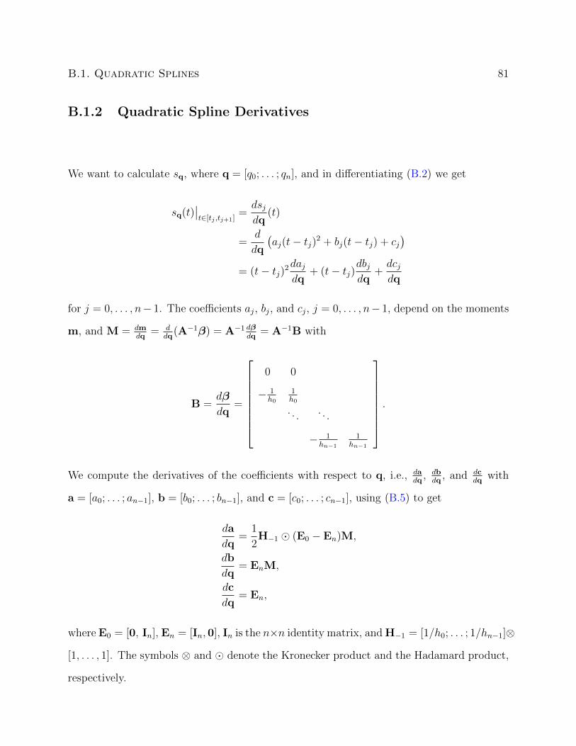
B.1. Quadratic Splines 81
B.1.2 Quadratic Spline Derivatives
We want to calculate sq, where q = [q0; . . . ; qn], and in differentiating (B.2) we get
sq(t)∣∣t∈[tj ,tj+1]
=dsjdq
(t)
=d
dq
(aj(t− tj)2 + bj(t− tj) + cj
)= (t− tj)2
dajdq
+ (t− tj)dbjdq
+dcjdq
for j = 0, . . . , n− 1. The coefficients aj, bj, and cj, j = 0, . . . , n− 1, depend on the moments
m, and M = dmdq
= ddq
(A−1β) = A−1 dβdq
= A−1B with
B =dβ
dq=
0 0
− 1h0
1h0
. . . . . .
− 1hn−1
1hn−1
.
We compute the derivatives of the coefficients with respect to q, i.e., dadq
, dbdq
, and dcdq
with
a = [a0; . . . ; an−1], b = [b0; . . . ; bn−1], and c = [c0; . . . ; cn−1], using (B.5) to get
da
dq=
1
2H−1 � (E0 − En)M,
db
dq= EnM,
dc
dq= En,
where E0 = [0, In], En = [In,0], In is the n×n identity matrix, and H−1 = [1/h0; . . . ; 1/hn−1]⊗
[1, . . . , 1]. The symbols ⊗ and � denote the Kronecker product and the Hadamard product,
respectively.
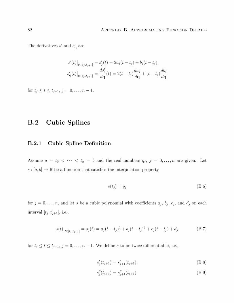
82 Appendix B. Approximating Function Details
The derivatives s′ and s′q are
s′(t)∣∣t∈[tj ,tj+1]
= s′j(t) = 2aj(t− tj) + bj(t− tj),
s′q(t)∣∣t∈[tj ,tj+1]
=ds′jdq
(t) = 2(t− tj)dajdq
+ (t− tj)dbjdq
for tj ≤ t ≤ tj+1, j = 0, . . . , n− 1.
B.2 Cubic Splines
B.2.1 Cubic Spline Definition
Assume a = t0 < · · · < tn = b and the real numbers qj, j = 0, . . . , n are given. Let
s : [a, b]→ R be a function that satisfies the interpolation property
s(tj) = qj (B.6)
for j = 0, . . . , n, and let s be a cubic polynomial with coefficients aj, bj, cj, and dj on each
interval [tj, tj+1], i.e.,
s(t)∣∣t∈[tj ,tj+1]
= sj(t) = aj(t− tj)3 + bj(t− tj)2 + cj(t− tj) + dj (B.7)
for tj ≤ t ≤ tj+1, j = 0, . . . , n− 1. We define s to be twice differentiable, i.e.,
s′j(tj+1) = s′j+1(tj+1), (B.8)
s′′j (tj+1) = s′′j+1(tj+1) (B.9)

B.2. Cubic Splines 83
for j = 0, . . . , n− 2, and we call s a cubic spline [27].
Equations (B.6), (B.8), and (B.9) provide 4n− 2 conditions for the 4n coefficients aj, bj, cj,
and dj, j = 0, . . . , n − 1. We uniquely determine s by choosing boundary conditions, e.g.,
not-a-knot boundary conditions, which are s′′′0 (t1) = s′′′1 (t1) and s′′′n−2(tn−1) = s′′′n−1(tn−1). For
efficient calculations of the coefficients aj, bj, cj, and dj, we define moments mj = s′′(tj)
for j = 0, . . . , n. The second derivative of s is linear in each interval [tj, tj+1] and must
satisfy (B.9), so for t ∈ [tj, tj+1], the piecewise second derivatives have the expression
s′′j (t) = mjtj+1 − thj
+mj+1t− tjhj
(B.10)
with hj = tj+1 − tj for j = 0, . . . , n− 1. Integrating (B.10) and using (B.6), we get
s′j(t) = −mj(tj+1 − t)2
2hj+mj+1
(t− tj)2
2hj+qj+1 − qj
hj− hj
6(mj+1 −mj),
and
sj(t) = mj(tj+1 − t)3
6hj+mj+1
(t− tj)3
6hj
+
(qj+1 − qj
hj− hj
6(mj+1 −mj)
)(t− tj) + qj −mj
h2j6
for j = 0, . . . , n− 1. Satisfying (B.8) dictates that
(1− λj+1)mj + 2mj+1 + λj+1mj+2 =6
hj + hj+1
(qj+2 − qj+1
hj+1
− qj+1 − qjhj
)
with λj+1 =hj+1
hj+hj+1for j = 0, . . . , n− 2.
We calculate moments m = [m0; . . . ;mn] by solving the linear system Am = β. In this

84 Appendix B. Approximating Function Details
case β = [β0; . . . ; βn] with βj+1 = 6hj+hj+1
(qj+2−qj+1
hj+1− qj+1−qj
hj
)for j = 0, . . . , n− 2 and
A =
A0
A
An
∈ R(n+1)×(n+1)
with
A =
1− λ1 2 λ1
. . . . . . . . .
1− λn−1 2 λn−1
.The boundary conditions determine the entries A0, An, β0, and βn, and
A0 =
[− 1
h0,
1
h0+
1
h1,− 1
h1, 0, . . . , 0
],
An =
[0, . . . , 0,− 1
hn−2,
1
hn−2+
1
hn−1,− 1
hn−1
],
β0 = βn = 0
for the not-a-knot conditions. With m given, we define the coefficients aj, bj, cj, and dj as
aj =mj+1 −mj
6hj,
bj =mj
2,
cj =qj+1 − qj
hj− (2mj +mj+1)hj
6,
dj = qj
(B.11)
for j = 0, . . . , n− 1.
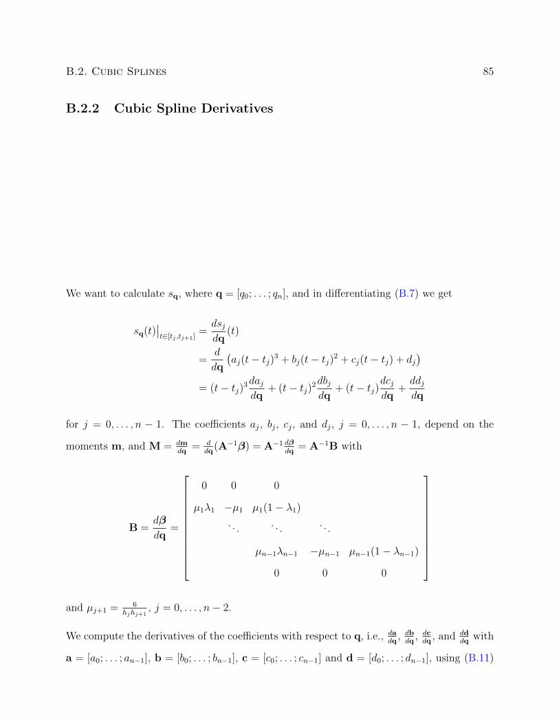
B.2. Cubic Splines 85
B.2.2 Cubic Spline Derivatives
We want to calculate sq, where q = [q0; . . . ; qn], and in differentiating (B.7) we get
sq(t)∣∣t∈[tj ,tj+1]
=dsjdq
(t)
=d
dq
(aj(t− tj)3 + bj(t− tj)2 + cj(t− tj) + dj
)= (t− tj)3
dajdq
+ (t− tj)2dbjdq
+ (t− tj)dcjdq
+ddjdq
for j = 0, . . . , n − 1. The coefficients aj, bj, cj, and dj, j = 0, . . . , n − 1, depend on the
moments m, and M = dmdq
= ddq
(A−1β) = A−1 dβdq
= A−1B with
B =dβ
dq=
0 0 0
µ1λ1 −µ1 µ1(1− λ1). . . . . . . . .
µn−1λn−1 −µn−1 µn−1(1− λn−1)
0 0 0
and µj+1 = 6
hjhj+1, j = 0, . . . , n− 2.
We compute the derivatives of the coefficients with respect to q, i.e., dadq
, dbdq
, dcdq
, and dddq
with
a = [a0; . . . ; an−1], b = [b0; . . . ; bn−1], c = [c0; . . . ; cn−1] and d = [d0; . . . ; dn−1], using (B.11)
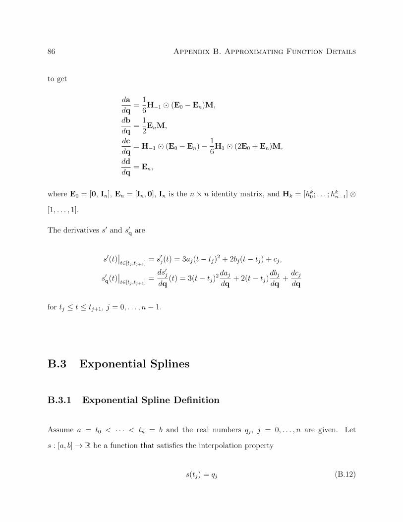
86 Appendix B. Approximating Function Details
to get
da
dq=
1
6H−1 � (E0 − En)M,
db
dq=
1
2EnM,
dc
dq= H−1 � (E0 − En)− 1
6H1 � (2E0 + En)M,
dd
dq= En,
where E0 = [0, In], En = [In,0], In is the n× n identity matrix, and Hk = [hk0; . . . ;hkn−1]⊗
[1, . . . , 1].
The derivatives s′ and s′q are
s′(t)∣∣t∈[tj ,tj+1]
= s′j(t) = 3aj(t− tj)2 + 2bj(t− tj) + cj,
s′q(t)∣∣t∈[tj ,tj+1]
=ds′jdq
(t) = 3(t− tj)2dajdq
+ 2(t− tj)dbjdq
+dcjdq
for tj ≤ t ≤ tj+1, j = 0, . . . , n− 1.
B.3 Exponential Splines
B.3.1 Exponential Spline Definition
Assume a = t0 < · · · < tn = b and the real numbers qj, j = 0, . . . , n are given. Let
s : [a, b]→ R be a function that satisfies the interpolation property
s(tj) = qj (B.12)
B.3. Exponential Splines 87
for j = 0, . . . , n, and let s be the sum of a linear and exponential function with coefficients
aj, bj, cj, and dj and known positive exponential coefficient pj, on each interval [tj, tj+1], i.e.,
s(t)∣∣t∈[tj ,tj+1]
= sj(t) = aj + bj(t− tj) + cjepj(t−tj) + dje
−pj(t−tj) (B.13)
for tj ≤ t ≤ tj+1, j = 0, . . . , n− 1. We define s to be twice differentiable, i.e.,
s′j(tj+1) = s′j+1(tj+1), (B.14)
s′′j (tj+1) = s′′j+1(tj+1) (B.15)
for j = 0, . . . , n−2, and we call s an exponential spline. This representation of an exponential
spline is not numerically well-behaved in cases where pj → 0 or pj → ∞ [64]. We can
rewrite (B.13) by changing the basis and redefining the coefficients aj, bj, cj, and dj as
s(t)∣∣t∈[tj ,tj+1]
= sj(t) = aj(t− tj) + bj(tj+1 − t)+
cj sinh(pj(t− tj)) + dj sinh(pj(tj+1 − t)). (B.16)
Equations (B.12), (B.14), and (B.15) provide 4n− 2 conditions for the 4n coefficients aj, bj,
cj, and dj, j = 0, . . . , n− 1. We uniquely determine s by choosing boundary conditions, e.g.,
not-a-knot boundary conditions, which are s′′′0 (t1) = s′′′1 (t1) and s′′′n−2(tn−1) = s′′′n−1(tn−1). For
efficient calculations of the coefficients aj, bj, cj, and dj, we define moments mj = s′′(tj) for
j = 0, . . . , n. The second derivative of s is a combination of the hyperbolic sine functions
in each interval [tj, tj+1] and must satisfy (B.15), so for t ∈ [tj, tj+1], the piecewise second
derivatives have the expression
s′′j (t) = mj+1sinh(pj(t− tj))
sinh(pjhj)+mj
sinh(pj(tj+1 − t))sinh(pjhj)
(B.17)
88 Appendix B. Approximating Function Details
with hj = tj+1 − tj for j = 0, . . . , n− 1. Integrating (B.17) and using (B.12), we get
s′j(t) =mj+1
pj
cosh(pj(t− tj))sinh(pjhj)
− mj
pj
cosh(pj(tj+1 − t))sinh(pjhj)
+qj+1 − qj
hj− mj+1 −mj
p2jhj
and
sj(t) =mj+1
p2j
sinh(pj(t− tj))sinh(pjhj)
+mj
p2j
sinh(pj(tj+1 − t))sinh(pjhj)
+(qj+1 − qj
hj− mj+1 −mj
p2jhj
)(t− tj) + qj −
mj
p2j.
for j = 0, . . . , n− 1. Satisfying (B.14) dictates that
λj+1mj + (µj+1 + µj+2)mj+1 + λj+2mj+2 =qj+2 − qj+1
hj+1
− qj+1 − qjhj
with
λj+1 =sinh(pjhj)− pjhjp2jhj sinh(pjhj)
,
µj+1 =pjhj cosh(pjhj)− sinh(pjhj)
p2jhj sinh(pjhj)
for j = 0, . . . , n− 2.
We calculate the moments m = [m0; . . . ;mn] by solving the linear system Am = β. In this
case β = [β0; . . . ; βn] with βj+1 =qj+2−qj+1
hj+1− qj+1−qj
hjfor j = 0, . . . , n− 2 and
A =
A0
A
An
∈ R(n+1)×(n+1)

B.3. Exponential Splines 89
with
A =
λ1 µ1 + µ2 λ2
. . . . . . . . .
λn−2 µn−2 + µn−1 λn−1
.The boundary conditions determine the entries A0, An, β0, and βn, and
A0 =
[− p0
sinh(p0h0),p0 cosh(p0h0)
sinh(p0h0)+p1 cosh(p1h1)
sinh(p1h1),− p1
sinh(p1h1), 0, . . . , 0
],
An =
[0, . . . , 0,− pn−2
sinh(pn−2hn−2),pn−2 cosh(pn−2hn−2)
sinh(pn−2hn−2)+pn−1 cosh(pn−1hn−1)
sinh(pn−1hn−1),− pn−1
sinh(pn−1hn−1)
],
β0 = βn = 0.
for the not-a-knot conditions. With m given, we define the coefficients aj, bj, cj, and dj as
aj =qj+1
hj− mj+1
p2jhj,
bj =qjhj− mj
p2jhj,
cj =mj+1
p2j sinh(pjhj),
dj =mj
p2j sinh(pjhj)
(B.18)
for j = 0, . . . , n− 1.

90 Appendix B. Approximating Function Details
B.3.2 Exponential Spline Derivatives
We want to calculate sq, where q = [q0; . . . ; qn], and in differentiating (B.16) we get
sq(t)∣∣t∈[tj ,tj+1]
=dsjdq
(t)
=d
dq(aj(t− tj) + bj(tj+1 − t) + cj sinh(pj(t− tj)) + dj sinh(pj(tj+1 − t)))
= (t− tj)dajdq
+ (tj+1 − t)dbjdq
+ sinh(pj(t− tj))dcjdq
+ sinh(pj(tj+1 − t))ddjdq
for j = 0, . . . , n − 1. The coefficients aj, bj, cj, and dj, j = 0, . . . , n − 1, depend on the
moments m, and M = dmdq
= ddq
(A−1β) = A−1 dβdq
= A−1B with
B =dβ
dq=
0 0 0
1h0− 1h0− 1
h11h1
. . . . . . . . .
1hn−2
− 1hn−2− 1
hn−1
1hn−1
0 0 0
.
We compute the derivatives of the coefficients with respect to q, i.e., dadq
, dbdq
, dcdq
, and dddq
with
a = [a0; . . . ; an−1], b = [b0; . . . ; bn−1], c = [c0; . . . ; cn−1] and d = [d0; . . . ; dn−1], using (B.18)
to get
da
dq= H−1 � (E0 −P−2 � E0M),
db
dq= H−1 � (En −P−2 � EnM),
dc
dq= P−2 � S� E0M,
dd
dq= P−2 � S� EnM,
B.4. Hermite Cubic Splines 91
where E0 = [0, In], En = [In,0], In is the n× n identity matrix, H−1 = [1/h0; . . . ; 1/hn−1]⊗
[1, . . . , 1], P−2 = [1/p20; . . . ; 1/p2n−1]⊗[1, . . . , 1], and S = [1/ sinh(p0h0); . . . ; 1/ sinh(pn−1hn−1)]⊗
[1, . . . , 1].
We define the derivatives s′ and s′q as
s′(t)∣∣t∈[tj ,tj+1]
= s′j(t) = aj − bj + cjpj cosh(pj(t− tj))− djpj cosh(pj(tj+1 − t)),
s′q(t)∣∣t∈[tj ,tj+1]
=ds′jdq
(t) =dajdq− dbjdq
+ pj cosh(pj(t− tj))dcjdq− pj cosh(pj(tj+1 − t))
ddjdq
for tj ≤ t ≤ tj+1, j = 0, . . . , n− 1.
B.4 Hermite Cubic Splines
B.4.1 Hermite Cubic Spline Definition
Assume a = t0 < · · · < tn = b and the real numbers qj and rj, j = 0, . . . , n are given. Let
s : [a, b]→ R be a function that satisfies the interpolation properties
s(tj) = qj, (B.19)
s′(tj) = rj (B.20)
for j = 0, . . . , n, and let s be a cubic polynomial with coefficients aj, bj, cj, and dj on each
interval [tj, tj+1], i.e.,
s(t)∣∣t∈[tj ,tj+1]
= sj(t) = aj(t− tj)3 + bj(t− tj)2 + cj(t− tj) + dj (B.21)
for tj ≤ t ≤ tj+1, j = 0, . . . , n− 1. We call s a Hermite cubic spline [74].

92 Appendix B. Approximating Function Details
Equations (B.19) and (B.20) provide 4n conditions for the 4n coefficients aj, bj, cj, and dj,
j = 0, . . . , n− 1, so the given information uniquely determines s. We define the coefficients
aj, bj, cj, and dj as
aj =2(qj − qj+1)
h3j+rj + rj+1
h2j,
bj =3(qj+1 − qj)
h2j− rj + 2rj+1
hj,
cj = rj,
dj = qj
(B.22)
with hj = tj+1 − tj for j = 0, . . . , n− 1.
B.4.2 Hermite Cubic Spline Derivatives
We want to calculate sv, where v = [q0; . . . ; qn; r0; . . . ; rn], and in differentiating (B.21) we
get
sv(t)∣∣t∈[tj ,tj+1]
=dsjdv
(t)
=d
dv
(aj(t− tj)3 + bj(t− tj)2 + cj(t− tj) + dj
)= (t− tj)3
dajdv
+ (t− tj)2dbjdv
+ (t− tj)dcjdv
+ddjdv
for j = 0, . . . , n− 1.
We compute the derivatives of the coefficients with respect to v, i.e., dadv
, dbdv
, dcdv
, and dddv
, with
a = [a0; . . . ; an−1], b = [b0; . . . ; bn−1], c = [c0; . . . ; cn−1] and d = [d0; . . . ; dn−1], using (B.22)
B.4. Hermite Cubic Splines 93
to get
da
dv= [2H−3 � (En − E0),H−2 � (En + E0)]
db
dv= [3H−2 � (E0 − En),−H−1 � (En + 2E0)]
dc
dv= [0,En]
dd
dv= [En,0]
where E0 = [0, In], En = [In,0], In is the n× n identity matrix, and Hk = [hk0; . . . ;hkn−1]⊗
[1, . . . , 1].
The derivatives s′ and s′v are
s′(t)∣∣t∈[tj ,tj+1]
= s′j(t) = 3aj(t− tj)2 + 2bj(t− tj) + cj,
s′v(t)∣∣t∈[tj ,tj+1]
=ds′jdv
(t) = 3(t− tj)2dajdv
+ 2(t− tj)dbjdv
+dcjdv
for tj ≤ t ≤ tj+1, j = 0, . . . , n− 1.