parameter estimation for inventory of load models in electric … · parameter estimation for...

Parameter Estimation for Inventory of LoadModels in Electric Power Systems

Amit Patel, Kevin Wedeward, and Michael Smith

Abstract—This paper presents an approach to characterizepower system loads through estimation of contributions from in-dividual load types. In contrast to methods that fit one aggregatemodel to observed load behavior, this approach estimates theinventory of separate components that compose the total powerconsumption. Common static and dynamic models are used torepresent components of the load, and parameter estimationis used to determine the amount each load contributes tothe cumulative consumption. Trajectory sensitivities form thebasis of the parameter estimation algorithm and give insightinto which parameters are well-conditioned for estimation.Parameters of interest are contributions to total load andinitial conditions for dynamic loads. Results are presented forsimulated data to demonstrate the feasibility of the approach.

Index Terms—electric power systems, load modeling, simu-lation, trajectory sensitivities, parameter estimation.

I. INTRODUCTION

As power system models and simulations used for plan-ning and stability studies become more advanced, higherfidelity models of all power system components are needed.Loads are particularly difficult to describe due to their diversecomposition and variation in time, yet their importance tovoltage stability and transient behavior has been recognized[1]–[4]. The approaches to load modeling can be catego-rized as either measurement-based or component-based [4].Measurement-based approaches utilize data collected froma substation or feeder to develop a model that matchesobserved behavior (see, for example, [5]–[7]). Component-based approaches combine known models of all devices thatmake up the load (see, for example, [2], [4]). A combinationof the approaches, known as identification of load inventory,has been developed where measurements are used to estimatethe fraction (percentage) that each different device within aload contributes to the aggregate power consumed [8], [9].

The focus of this paper is development of a load inventorymodel where parameter estimation is used to determinethe amount each component contributes to the total powerconsumption. Parameter estimation is achieved via a Gauss-Newton method based upon trajectory sensitivities (see [10])which computes parameters that best fit simulated modelresponses to simulated measurements on a single phase. Theresults indicate which load contributions are well-conditionedfor estimation and that those parameters can be accuratelyestimated in the presence of measurement error. Initial con-ditions of the dynamic states in the load models are difficultto identify; however, the load contribution coefficients areidentifiable.

Manuscript submitted on July 13, 2014.Amit Patel is with Accenture, Irving, TX 75039 USA.Kevin Wedeward and Michael Smith are with the Institute for Complex

Additive Systems Analysis (ICASA), New Mexico Institute of Mining andTechnology, Socorro, NM 87801 USA, email: [email protected].

II. LOAD MODELING

A wide variety of load models exist to mathematicallyrepresent the power consumed by a load and its dependencieson voltage, frequency, type and composition. Three commonmathematical models for loads in power systems are pre-sented below and utilized in the proposed approach. In allcases, it is assumed that powers and voltages are normalizedby base values such that their units are in per unit (p.u.) [11].

A. ZIP

A polynomial model is commonly used to represent loadsand capture their voltage dependency. The average andreactive powers of the load are written as a sum of constantimpedance (Z), constant current (I) and constant power (P),and referred to as the ZIP model [3], [11].

P = P0(K1p

(V

V0

)2

+K2pV

V0+K3p) (1)

Q = Q0(K1q

(V

V0

)2

+K2qV

V0+K3q) (2)

where P , Q are the average and reactive power consumedby the load, respectively, P0, Q0 represent the nominalaverage and reactive power of the load, respectively, V is themagnitude of the sinusoidal voltage at the bus to which theload is connected, V0 is the magnitude of the nominal voltageat the bus, and coefficients K1p, K2p, K3p, K1q , K2q andK3q define the proportion of each component of the model.Coefficients for many load types have been experimentallydetermined and reported [2], [4], [5].

B. Exponential Recovery

The power profile is defined by

P =xpTp

+ P0

(V

V0

)αt(3)

Q =xqTq

+Q0

(V

V0

)βt(4)

where P , Q are the average and reactive power consumedby the load, respectively, P0, Q0 are the nominal averageand reactive power, respectively, V is the magnitude of thesinusoidal voltage at the bus to which the load is connected,and V0 is the magnitude of the nominal voltage at the bus.Parameters Tp and Tq are the average and reactive load re-covery time constants, respectively, αs and βs are the steady-state dependence of average and reactive powers on voltage,respectively, and αt and βt are the transient dependence ofaverage and reactive powers on voltage, respectively. Theparameters govern the behavior of the load model, and aregenerally fit to measurements. States xp and xq are average

Proceedings of the World Congress on Engineering and Computer Science 2014 Vol I WCECS 2014, 22-24 October, 2014, San Francisco, USA

ISBN: 978-988-19252-0-6 ISSN: 2078-0958 (Print); ISSN: 2078-0966 (Online)

WCECS 2014

and reactive power recovery, respectively, and are governedby the differential equations [7], [12], [13]:

xp =−xpTp

+ P0

((V

V0

)αs−(V

V0

)αt)(5)

xq =−xqTq

+Q0

((V

V0

)βs−(V

V0

)βt). (6)

Parameters for different load types have been experimentallydetermined and reported [7], [13].

C. Induction Motor

The induction motor’s voltages of interest are V ejθ =V cos(θ) + jV sin θ at the stator terminal and V ′ejθ

′=

v′d + jv′q at the voltage behind transient reactance. The

stator current is I = id + jiq = V ejθ−V ′ejθ′

Rs+jX′s

whereX ′s = Xs + XrXm

Xr+Xmis the transient reactance. Additional

parameters are stator resistance and leakage reactance, Rsand Xs, respectively, magnetizing reactance, Xm, and rotorresistance and leakage reactance, Rr, Xr, respectively.

The voltage V ′ejθ′

= v′d + jv′q has real and imaginaryparts governed by the differential equations [11], [14]

dv′ddt

= − RrXr +Xm

[v′d +

(X2m

Xr +Xm

)iq

]+ sv′q(7)

dv′qdt

= − RrXr +Xm

[v′q −

(X2m

Xr +Xm

)id

]− sv′d(8)

ds

dt=

1

2H

(Tmo (1− s)2 − Te

)(9)

where s = ωs−ωrωs

is slip, ωr is rotor speed, ωs is angularvelocity of the stator field, Tmo is a load torque constant,Te = v′did + v′qiq is electromagnetic torque, and H is themotor and motor load inertia.

The average power P and reactive power Q consumed bythe motor are then given by

P = Re(V ejθI∗)

=1

R2s +X ′2s

(Rs(V

2 + V cos(θ)v′d − V sin(θ)v′q)

−X ′s(V cos(θ)v′q − V sin(θ)v′d))

(10)

Q = Im(V ejθI∗)

=1

R2s +X ′2s

(Rs(V cos(θ)v′q − V sin(θ)v′d)

+X ′s(V2 − V cos(θ)v′d − V sin(θ)v′q)

)(11)

where (·)∗ denotes complex conjugate of the complex quan-tity, Re(·) and Im(·) denote the real and imaginary partsof a complex number, respectively. Parameters for differentload types have been experimentally determined and reported[11], [15], [16].

D. Load Inventory Concept

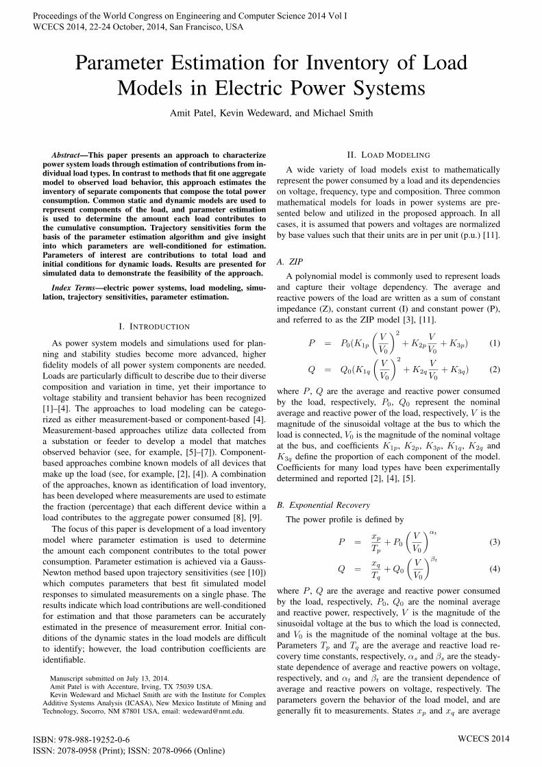
Load behavior will be modeled by using an aggregationof ZIP, exponential recovery and induction motor modelsfrom above with appropriate parameters selected for each torepresent the load’s components. This is shown conceptuallyin Figure 1 with the total complex power consumed PL+jQLthe sum of the power consumed by all the individual loadelements. The parameters of interest will be the contribution

Load 1µ1(P1 + jQ1)

Load 2µ2(P2 + jQ2)

...

Load NLµNL(PNL + jQNL)

V ejθ

PL + jQL

Fig. 1. Concept of load inventory

coefficients µi for i = 1, 2, . . . , NL where NL is the numberof unique types of loads assumed to be connected to the busas well as the initial conditions needed for each dynamicmodel.

In summary, the aggregate load with average power PLand reactive power QL will be the fractional sum of eachindividual type of model. Each model represents a candidateload that might exist in the inventory and its fractionalcontribution indicated by µi is the parameter of interestfor determining the inventory of loads. Total (aggregate)complex power is the sum of all load powers

PL + jQL = µ1(P1 + jQ1) + µ2(P2 + jQ2)

+ · · ·+ µNL(PNL + jQNL). (12)

III. TRAJECTORY SENSITIVITIES

Differential-algebraic models are often utilized to repre-sent the dynamic behavior of electric power systems [17].When all loads are taken at a bus for the load inventoryapproach, the combined models presented above for loadscan be represented in a manner similar to that of the broaderpower system:

x = f(x, V ) (13)y = g(x, V, µ). (14)

Here x is the vector of dynamic states (e.g., xp, xq , v′d, v′q ,s for dynamic loads) that satisfy the differential equations(13), y = [PL, QL]T is the 2 × 1 vector of total averageand reactive powers consumed by the aggregate load, V isthe magnitude of the voltage at the bus (treated as an input)and µ is the vector of contributions µi=1,2,...,NL taken asparameters.

Trajectory sensitivities provide a means to quantify theeffect of small changes in parameters and/or initial conditionson a dynamic system’s trajectory. Trajectory sensitivities willbe utilized to guide the choice of how the parameters (heretaken to be contributions µ and initial conditions x0) shouldbe altered to “best” match simulated trajectories to measure-ments of average power and reactive power consumed bythe aggregate load. Following the presentation of trajectorysensitivities in [10], [17], flows of x and y that describe the



WCECS 2014

response of (13), (14) are defined as

x(t) = φx(λ, V, t) (15)y(t) = g(φx(λ, V, t), λ, V, t) = φy(λ, V, t) (16)

where x(t) satisfies (13), all parameters of interest are com-bined into the vector λ = [x0, µ]T of dimension M×1, andflows show the dependence of the trajectories on parametersλ (here initial conditions and fractional contributions), inputV and time t. To obtain the sensitivity of the trajectoriesto small changes in the parameters ∆λ, a Taylor seriesexpansion of (15), (16) can be formed. Neglecting higherorder terms in the expansion yields

∆x(t) = φx(λ+ ∆λ, V, t)− φx(λ, V, t) (17)

≈ ∂φx(λ, V, t)

∂λ∆λ ≡ xλ(t)∆λ (18)

∆y(t) = φy(λ+ ∆λ, V, t)− φy(λ, V, t) (19)

≈ ∂φy(λ, V, t)

∂λ∆λ ≡ yλ(t)∆λ. (20)

The time-varying partial derivatives xλ and yλ are known asthe trajectory sensitivities, and can be obtained by differen-tiating (13) and (14) with respect to λ. This differentiationgives

xλ = fx(t)xλ (21)yλ = gx(t)xλ + gλ(t) (22)

where fx ≡ ∂f∂x , gx ≡ ∂g

∂x and gλ ≡ ∂g∂λ are time-varying

Jacobian matrices, and fλ ≡ ∂f∂λ = 0. Along the trajectory

of the aggregate loads described by (13), (14) the trajectorysensitivities will evolve according to the linear, time-varyingdifferential equations (21), (22). Initial conditions for xλ areobtained from (15) by noting x(t0) = φx(λ, V, t0) = x0 suchthat xλ(t0) = I where I is the identity matrix [10]. Initialconditions for yλ follow directly from the algebraic equation(22) to yield yλ(t0) = gx(t0) + gλ(t0).

The N × M sensitivity matrix for the ith output yi isnow defined by taking sensitivities (22) at discrete timestk=0,1,...,N−1

Si(λj) =

yiλ(t0)

yiλ(t1)...

yiλ(tN−1)

(23)

where N is the number of discrete values of time at whichvalues are taken from the trajectory sensitivity (22) found bynumerically solving the coupled system (13), (14), (21), (22);M is the number of parameters in λ; λj is the particular setof values for parameters used when computing the trajectoryand associated sensitivities; and for this particular applicationy1λ = PLλ , y2λ = QLλ and the complete sensitivity matrix

S(λj) =

[S1(λj)

S2(λj)

]is of dimension 2N ×M .

As an example of computing the equations that will besolved for trajectory sensitivities, assume the total power isgiven by (12) and P1, Q1 are consumed by a load representedas the exponential recovery model’s powers (3), (4). The

sensitivities of PL, QL to parameter µ1 are∂PL∂µ1

≡ PLµ1 = P1 =xpTp

+ P0

(VV0

)αt(24)

∂QL∂µ1

≡ QLµ1 = Q1 =xqTq

+Q0

(VV0

)βt(25)

where the states xp, xq will come from numerical solutionof (5), (6) and V will be a specified input. The sensitivitiesof PL, QL to the initial conditions xp(0), xq(0) are

∂PL∂xp(0)

≡ PLxp(0) = µ11Tp

∂xp∂xp(0)

= µ11Tpxpxp(0) (26)

∂PL∂xq(0)

≡ PLxq(0) = 0 (27)

∂QL∂xp(0)

≡ QLxp(0) = 0 (28)

∂QL∂xq(0)

≡ QLxq(0) = µ11Tq

∂xq∂xq(0)

= µ11Tqxqxq(0) (29)

where the sensitivities xpxp(0) ≡∂xp∂xp(0)

, xqxq(0) ≡∂xq∂xq(0)

willbe the solution to the following differential equations thatgovern the trajectory sensitivities found by differentiating (5),(6) with respect to the initial conditions xp(0), xq(0)

∂

∂xp(0)xp ≡ xpxp(0) = − 1

Tp

∂xp∂xp(0)

= − 1Tpxpxp(0) (30)

∂

∂xq(0)xp ≡ xpxq(0) = 0 (31)

∂

∂xp(0)xq ≡ xqxp(0) = 0 (32)

∂

∂xq(0)xq ≡ xqxq(0) = − 1

Tq

∂xq∂xq(0)

= − 1Tqxqxq(0) . (33)

Note the order of the derivatives (with respect to parameterand time) were interchanged in the process.

The differential equations (30), (33) that govern the trajec-tory sensitivities are solved numerically in parallel with thedifferential equations (5), (6) that govern the model such thattrajectories are obtained for both. Calculations of sensitivitiesfor all load models to all parameters are given in [18].

IV. PARAMETER ESTIMATION

Parameter estimation will be cast as a nonlinear leastsquares problem and solved using a Gauss-Newton iterativeprocedure [17]. Measurements of average and reactive powerconsumed by a load during a disturbance will be used toestimate the unknown model parameters (here contributionsand initial conditions). The aim of parameter estimation isto determine parameter values that achieve the closest matchbetween the measured samples and the model’s simulatedtrajectory. Let measurements of the total average powerPL and reactive power QL (denoted by PLm and QLm ,respectively) consumed by the aggregate load be given bythe appended sequences of N measurements

~ym =

[[PLm(t0), PLm(t1), . . . , PLm(tN−1)]

T

[QLm(t0), QLm(t1), . . . , QLm(tN−1)]T

](34)

with the corresponding simulated trajectory from numericallysolving (13), (14) given by

~y =

[[PL(t0), PL(t1), . . . , PL(tN−1)]

T

[QL(t0), QL(t1), . . . , QL(tN−1)]T

](35)



WCECS 2014

to get corresponding values at times tk=0,1,2,...,N−1. Themismatch between the measurements and correspondingmodel’s trajectory can be written in vector form as

~e(λ) = ~y(λ)− ~ym (36)

where the notation is used to show the dependence of thetrajectory, and correspondingly the error, on the parametersλ. The vectors ~e, ~y and ~ym will be of dimension 2N×1 as Nmeasurements of PL and QL are assumed. The best matchbetween model and measurement is obtained by varying theparameters so as to minimize the error vector ~e(λ) by somemeasure. One common measure is the two-norm (sum ofsquares) of the error vectors expressed as a cost function

C(λ) =1

2‖~e(λ)‖22 =

1

2

∑2N−1

k=0ek(λ)2. (37)

The error ek(λ) is the kth element of ~e and can be linearlyapproximated via a Taylor series expansion about an initialvalue of λ = λj which yields

ek(λ) ≈ ek(λj) +∂ek(λj)

∂λ(λ− λj) (38)

= ek(λj) + yλk(λj)∆λ (39)

where ∂ek(λj)

∂λ = ∂yk(λj)

∂λ = yλk(λj) since the measurementsymk are independent of λ and the definition ∆λ = λ−λj isutilized. The new value of λj denoted λj+1 will be chosento minimize the following cost function with linearized error.

C(λ) =1

2

∑2N−1

k=0(ek(λj) + yλk(λj)∆λ)2

=1

2

∑2N−1

k=0(ek(λj) + Sk(λj)∆λ)2

=1

2

∥∥~e(λj) + S(λj)∆λ∥∥22

(40)

where Sk is the kth row of the sensitivity matrix S.Minimizing the cost function of linearized error (40) can

now be performed via the Gauss-Newton method [17]. Theprocess starts with an initial guess λ0 for parameter valuesand then parameters are updated according to iterations ofthe following two steps.

S(λj)TS(λj)∆λj+1 = −S(λj)T e(λj) (41)λj+1 = λj + αj+1∆λj+1 (42)

where S is the trajectory sensitivity matrix defined in (23),αj+1 is a scalar that determines step size, and iterations stopwhen ∆λj+1 is sufficiently small. The resulting parametervalues λj+1 will be a local minimum for the cost function(37) due to the linearization and will be dependent on theinitial guess λ0. An additional note is that the parameterestimation process breaks down if STS is ill-conditioned,i.e., nearly singular. This leads to the concept of identifia-bility and quantification of parametric effects [17], [19]. Theinvertibility of STS can be investigated through its singularvalues and condition number, eigenvalues, or magnitudeof sensitivities over a trajectory via the 2-norm. The less-rigorous, 2-norm will be utilized here to gain insight intothe condition of STS. The 2-norm will be defined for thesensitivity of the ith output yi to the jth parameter λjsummed over discrete times tk as∥∥Sij∥∥2

2=N−1∑k=0

Sij(tk, λ)2. (43)

The size of the values computed via (43) will give anindication of the effect of parameters on the trajectory, and inturn give guidance as to which parameters can be estimated.

V. EXAMPLE OF APPLICATION VIA SIMULATION

The parameter estimation approach described above wasimplemented through simulation to estimate load contribu-tions and initial conditions. Five loads, each represented byone of five models, were taken as connected to a bus asshown in Figure 1 with magnitude V of the bus’s phasorvoltage taken to be the input to the models, and averageand reactive powers PL, QL, respectively, taken to be the(measurable) outputs. Load 1 was an exponential recoverymodel, load 2 was the model of a residential induction motor,load 3 was a model of a small industrial induction motor,load 4 was a model of a large industrial induction motor, andload 5 was a ZIP model. That made the M = 16 unknownparameters

λ =[xp1(0), xq1(0), v′d2(0), v′q2(0), s2(0), v′d3(0), v′q3(0),

s3(0), v′d4(0), v′q4(0), s4(0), µ1, µ2, µ3, µ4, µ5

]T(44)

which includes initial conditions for all the states in theindividual models as well as the fractional contributions ofeach load model to the aggregate power consumed. For thefive loads considered, the total load is given by

PL + jQL = µ1(P1 + jQ1) + µ2(P2 + jQ2)

+ µ3(P3 + jQ3) + µ4(P4 + jQ4)

+ µ5(P5 + jQ5) (45)

with NL = 5; µi=1,2,...,5 the fractional contributions ofeach load model; P1, Q1 given by (3), (4); P2, Q2 given by(10), (11); P3, Q3 given by (10), (11); P4, Q4 given by (10),(11); and P5, Q5 given by (1), (2). Representative values forparameters used in each model were taken from [4], [13],[16] and are given in Table I, and the nominal bus voltageis taken to be V0 = 1p.u.

TABLE IPARAMETER VALUES FOR MODELS OF LOADS

Load Model and Parameters

1 Exponential RecoveryP0 TP αs αt Q0 Tq βs βt

1.25 60 0 2 0.5 60 0 22 Induction Motor - Residential

Rs Xs Xm Rr Xr H T0

0.077 0.107 2.22 0.079 0.098 0.74 0.463 Induction Motor - Small Industrial

Rs Xs Xm Rr Xr H T0

0.031 0.1 3.2 0.018 0.18 0.7 0.64 Induction Motor - Large Industrial

Rs Xs Xm Rr Xr H T0

0.013 0.067 3.8 0.009 0.17 1.5 0.85 ZIP

P0 K1p K2p K3p Q0 K1q K2q K3q

1.0 0.15 0.6 0.25 0.7 0.05 -0.05 1.0

A. Results when no error in measurements

For study in simulation, a 3% decrease in the magnitudeof the bus’s voltage V was taken to be the input. The voltage



WCECS 2014

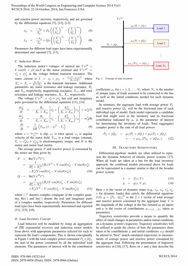
was dropped from its nominal value of 1p.u. to 0.97p.u. at 50seconds. With the initial conditions and load contributions atspecified values, the simulation was run to generate synthetic,“measured” data to represent data that might be collected bya voltage disturbance monitor or phasor measurement unit. Asampling rate of 10Hz was used to record the total averageand reactive powers consumed by the five loads. Nominalvalues for parameters are given in Table II, and plots of theaggregate power consumption PL and QL are given in Figure2 as the solid lines.

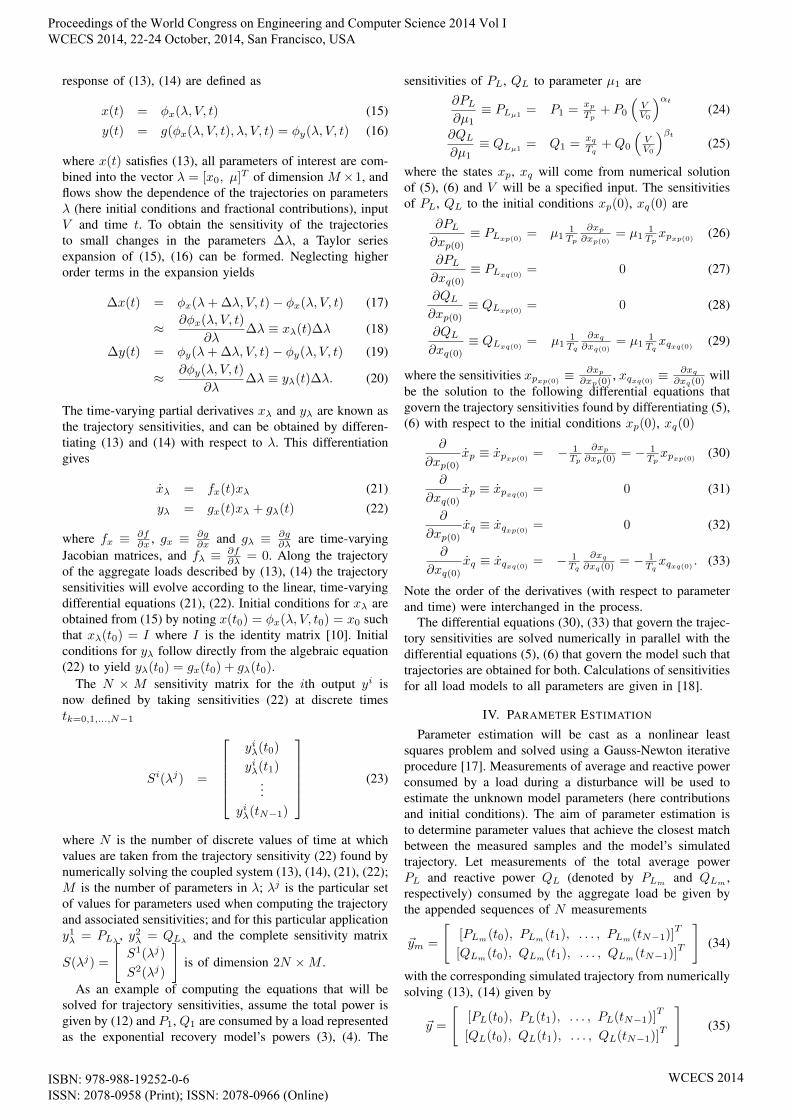
The simulation was then modified to run with initialguesses for parameter values, and the iterative Gauss-Newtonprocess described by (41), (42) implemented to update thevalues of the parameters until they converged to within aspecified tolerance. At each iteration, the system’s model(13), (14) and trajectory sensitivities (21), (22) were nu-merically solved using Matlab’s ode15s() solver for a newtrajectory using updated values of the parameters. The resultsof the iterative process can be seen Figure 3 and showconvergence of the load contributions to values used to createthe synthetic measurements. The final, estimated values of allparameters (both initial conditions and load contributions) aregiven in Table II. The simulated trajectories for PL and QLas the parameters are updated can be seen as the dashed linesin Figure 2.

TABLE IIVALUES, GUESSES AND ESTIMATES OF PARAMETERS

Load Model and Estimated Parameters

1 Exponential Recoveryxp(0) xq(0) µ1

value: 0.0010 0.0007 0.1000guess: 0.0025 0.0015 0.3000estimate: 0.0010 0.0007 0.1000

2 Induction Motor - Residentialv′d(0) v′q(0) s(0) µ2

value: 0.8659 0.1439 0.0399 0.2000guess: 0.9000 0.1800 0.0550 0.3000estimate: 0.8659 0.1439 0.0399 0.2001

3 Induction Motor - Small Industrialv′d(0) v′q(0) s(0) µ3


4 Induction Motor - Large Industrialv′d(0) v′q(0) s(0) µ4


5 ZIPµ5

value: 0.2000guess: 0.1000estimate: 0.2000

B. Study of identifiability

For the sample application above where no measurementerror was introduced, the 2-norm of all sensitivities wascalculated and shown in Table III. Of particular note is thatthe sensitivities of the average and reactive power are atleast an order of magnitude larger for load contributions than

Fig. 2. Average power (left) and reactive power (right) consumed byaggregate load; simulated measurements are solid lines and trajectories forupdated parameter estimates are dashed lines

Fig. 3. Estimates of parameters (as markers/symbols) representing loadcontributions over iterations; dashed lines are actual values

initial conditions. This indicates that the load contributionshave a larger impact on the trajectory and in turn should bemore readily identified through parameter estimation. Whenno measurement error was assumed, both initial conditionsand load contributions were identified, but when randomerror was introduced (as discussed in the next section) theestimates of the initial conditions were inaccurate. The zeroentries in the table imply that the load models’ powers donot depend on that particular parameter.

As an additional check of identifiability for the parametersof interest, both the condition number and eigenvalues werecomputed for the matrix STS. The condition number was2.281×1015 with sensitivities for initial conditions includedwhich confirmed an ill-conditioned matrix and potential diffi-culty in estimating initial conditions. When sensitivities wereremoved from STS leaving only those to load contributions,the condition number improved to 202.4 which indicatedload contributions are identifiable. Eigenvalues of STS werecomputed and further confirmed identifiable parameters as



WCECS 2014

TABLE III2-NORM OF TRAJECTORY SENSITIVITIES FOR PARAMETERS (LOAD

CONTRIBUTIONS AND INITIAL CONDITIONS) OF INTEREST

Load Model and 2-norm of Trajectory Sensitivities

1 Exponential Recoveryxp(0) xq(0) µ1

‖SPL‖22: 0.029 0 7.920

‖SQL‖22: 0 0.027 15.37

2 Induction Motor - Residentialv′d(0) v′q(0) s(0) µ2

‖SPL‖22: 0.005 0.003 0.002 14.37

‖SQL‖22: 0.002 0.001 0.001 13.59

3 Induction Motor - Small Industrialv′d(0) v′q(0) s(0) µ3

‖SPL‖22: 0.001 0.003 0.002 1.116

‖SQL‖22: 0.081 0.003 0.008 3.220

4 Induction Motor - Large Industrialv′d(0) v′q(0) s(0) µ4

‖SPL‖22: 0.004 0.003 0.003 4.095

‖SQL‖22: 0.009 0.005 0.007 4.725

5 ZIPµ5

‖SPL‖22: 75.97

‖SQL‖22: 64.89

small eigenvalues were associated with the initial conditionsand much larger eigenvalues were associated with the loadcontributions.

C. Results with 2% random error in measurements

The study described above was repeated, but this timewith an error in each measurement achieved by adding anormally distributed random number to each measurementwith mean 0 and standard deviation 2%. The method ofestimating parameters worked well for the load contributions,but not the initial conditions. This is attributed to the issueswith identifiability discussed above. Table IV shows the“true values”, initial guesses and estimates of the parametersrepresenting load contributions in this case.

TABLE IVVALUES, GUESSES AND ESTIMATES OF PARAMETERS WHEN 2%

RANDOM ERROR IN MEASUREMENTS

Load Model and Estimated Parameters

1 Exponential Recoveryµ1 value guess estimate

0.1000 0.3000 0.12312 Induction Motor - Residential

µ2 value guess estimate0.2000 0.3000 0.1698

3 Induction Motor - Small Industrialµ3 value guess estimate

0.2000 0.1000 0.17404 Induction Motor - Large Industrial

µ4 value guess estimate0.3000 0.2000 0.3102

5 ZIPµ5 value guess estimate

0.2000 0.1000 0.2272

VI. CONCLUSION

This paper presented an application of trajectory sensitivi-ties and parameter estimation to estimate an aggregate load’scomposition. An example is presented using simulated datafor five types of loads modeled by an exponential recoverymodel, three induction motor models with different param-eters, and a ZIP model. Future work will be to incorporateand investigate additional models, and apply the approachto real data collected from a voltage disturbance monitor orphasor measurement unit.

REFERENCES

[1] A. Ellis, D. Kosterev, and A. Meklin, “Dynamic load models: Whereare we?” in Proceedings of the IEEE Power Engineering SocietyTransmission and Distribution Conference, May 2006.

[2] D. Kosterev, A. Meklin, J. Undrill, B. Lesieutre, W. Price, D. Chassin,R. Bravo, and S. Yang, “Load modeling in power system studies:WECC progress update,” in Proceedings of the IEEE Power and En-ergy Society General Meeting - Conversion and Delivery of ElectricalEnergy in the 21st Century, July 2008.

[3] IEEE Task Force on Load Representation for Dynamic Performance,“Load representation for dynamic performance analysis [of powersystems],” IEEE Transactions on Power Systems, vol. 8, no. 2, pp.472–482, May 1993.

[4] W. Price, K. Wirgau, A. Murdoch, J. V. Mitsche, E. Vaahedi, andM. El-Kady, “Load modeling for power flow and transient stabilitycomputer studies,” IEEE Transactions on Power Systems, vol. 3, no. 1,pp. 180–187, Feb 1988.

[5] A. Bokhari, A. Alkan, R. Dogan, M. Diaz-Aguilo, F. de Leon,D. Czarkowski, Z. Zabar, L. Birenbaum, A. Noel, and R. Uosef,“Experimental determination of the ZIP coefficients for modern res-idential, commercial, and industrial loads,” IEEE Transactions onPower Delivery, vol. 29, no. 3, pp. 1372–1381, June 2014.

[6] D. Han, J. Ma, R.-m. He, and Z.-Y. Dong, “A real application ofmeasurement-based load modeling in large-scale power grids and itsvalidation,” IEEE Transactions on Power Systems, vol. 24, no. 4, pp.1756–1764, Nov 2009.

[7] D. Karlsson and D. J. Hill, “Modelling and identification of nonlineardynamic loads in power systems,” IEEE Transactions on PowerSystems, vol. 9, no. 1, pp. 157–166, February 1994.

[8] D. R. Sagi, S. J. Ranade, and A. Ellis, “Evaluation of a loadcomposition estimation method using synthetic data,” in Proceedingsof the 37th Annual North American Power Symposium, October 2005.

[9] S. Ranade, D. Sagi, and A. Ellis, “Identifying load inventory frommeasurements,” in Proceedings of the IEEE Power and Energy SocietyTransmission and Distribution Conference and Exhibition, May 2006.

[10] I. A. Hiskens and M. A. Pai, “Power system applications of trajectorysensitivities,” in Proceedings of the Power Engineering Society WinterMeeting, 2002.

[11] P. Kundur, Power system stability and control, N. J. Balu and M. G.Lauby, Eds. McGraw-Hill, Inc., 1994.

[12] D. J. Hill, “Nonlinear dynamic load models with recovery for voltagestability studies,” IEEE Transactions on Power Systems, vol. 8, no. 1,pp. 166–176, Feb 1993.

[13] I. R. Navarro, “Dynamic load models for power systems - estimation oftime-varying parameters during normal operation,” PhD thesis, LundUniversity, Lund, Sweden, September 2002.

[14] A. Ellis, “Advanced load modeling in power systems,” PhD thesis,New Mexico State University, Las Cruces, NM, December 2000.

[15] F. Nozari, M. Kankam, and W. Price, “Aggregation of induction motorsfor transient stability load modeling,” IEEE Transactions on PowerSystems, vol. 2, no. 4, pp. 1096–1103, Nov 1987.

[16] IEEE Task Force on Load Representation for Dynamic Performance,“Standard load models for power flow and dynamic performancesimulation,” IEEE Transactions on Power Systems, vol. 10, no. 3, pp.1302–1313, Aug 1995.

[17] I. A. Hiskens, “Nonlinear dynamic model evaluation from disturbancemeasurements,” IEEE Transactions on Power Systems, vol. 16, no. 4,pp. 702–710, November 2001.

[18] A. Patel, “Parameter estimation for load inventory models in electricpower systems,” MS thesis, New Mexico Institute of Mining andTechnology, Socorro, NM, December 2008.

[19] J. Rose and I. A. Hiskens, “Estimating wind turbine parameters andquantifying their effects on dynamic behavior,” in Proceedings of theIEEE Power and Energy Society General Meeting - Conversion andDelivery of Electrical Energy in the 21st Century, July 2008.



WCECS 2014

parameter estimation for inventory of load models in electric … · parameter estimation for...

Documents