parameter and state estimation of nonlinear systems with
TRANSCRIPT

Parameter and state estimation
of nonlinear systems with
applications in neuroscience
Michelle Siu Tze Chong
Submitted in total fulfilment of the requirements of the degree of Doctor of
Philosophy
March 2013
Department of Electrical and Electronics Engineering
The University of Melbourne
Produced on archival quality paper
Abstract
The focus of this work is deterministic parameter and state estimation of nonlinear sys-
tems with applications to neuroscience. Estimation in neuroscience typically involves
the reconstruction of unmeasured neural activity from measurements of the human
brain. We envisage that estimation plays a crucial role in neuroscience because of the
possibility of creating new avenues for neuroscientific studies and for the development of
diagnostic, management and treatment tools for diseases such as Epilepsy and Parkin-
sons disease. One of the most used measurements is the electroencephalogram (EEG).
To this end, we consider lumped-parameter nonlinear models with EEG as the output,
known as neural mass models.
Four observers are proposed in this thesis: (1) a nonlinear observer, (2) robust
circle criterion observers, (3) an adaptive observer and (4) the supervisory observer.
These observers are synthesised for classes of nonlinear systems, that cover some of
the commonly used neural mass models. Two state observers are shown and designed
respectively, in Part I, to be robust towards input and measurement noise, as well
as small perturbations in parameters. In the absence of noise and perturbations, the
estimates converge exponentially to the true values. The convergence of estimates to
their true values is with some error in the presence of noise and perturbations. Chapter
3 presents a nonlinear observer specific to the class of neural mass models considered.
In Chapter 4, we propose robust circle criterion observers for a class of systems, that
covers all our examples. We extended available results in the literature such that they
can be synthesised for the neural mass models. The robustness of the designed state
observers towards parameter uncertainty motivates the estimation of both parameters
and states in Part II.
In Chapter 5, we design an adaptive observer for a class of interconnected neural
mass models. The convergence of the estimates is asymptotic. Finally, in Chapter 6,
we present an alternative method using a multiple-model architecture, known in the
literature as the supervisory framework. Under non-restrictive conditions, we guarantee
the practical convergence of parameters and states.

Declaration
This is to certify that
1. the thesis comprises only my original work towards the PhD except
where indicated in the Preface,
2. due acknowledgement has been made in the text to all other material
used,
3. this thesis is fewer than 100,000 words in length, exclusive of tables,
maps, bibliographies and appendicies.
Michelle S. Chong
Date: 26 March 2013

Preface
The material developed in this thesis is the result of original research, unless otherwise
stated, solely during the author’s candidature in the Department of Electrical and Elec-
tronic Engineering, the University of Melbourne under the supervision of Prof. Dragan
Nesic and Dr. Levin Kuhlmann. The results presented in this thesis have been ob-
tained in collaboration with the author’s supervisors and Dr. Romain Postoyan from
Centre de Recherche en Automatique de Nancy (CRAN), France. Some results were
also obtained in collaboration with Dr. Andrea Varsavsky, who was also a supervisor
when she was in the University of Melbourne.
The work presented in this thesis have been accepted or submitted for publication
in journals, as well as presented and accepted at international conferences:
1. M. Chong, R. Postoyan, D. Nesic, L. Kuhlmann and A. Varsavsky. ‘A robust
circle criterion observer with application to neural mass models’ in Automatica,
vol. 48, pp 2986-2989, 2012.
2. M. Chong, R. Postoyan, D. Nesic, L. Kuhlmann and A. Varsavsky. ‘Estimating
the unmeasured membrane potential of neuronal populations using a class of
deterministic nonlinear filters’ in the Journal of Neural Engineering, vol. 9., pp
026001, 2012.
3. M. Chong, D. Nesic, R. Postoyan and L. Kuhlmann. ‘Parameter and state
estimation of nonlinear systems using a multi-observer under the supervisory
framework’ - submitted to IEEE Transactions of Automatic Control.
4. M. Chong, R. Postoyan, D. Nesic, L. Kuhlmann and A. Varsavsky. ‘A non-
linear estimator for the activity of neuronal populations in the hippocampus’
in the Proceedings of 18th World Congress of the International Federation of
Automatic Control (IFAC), 2011.
5. M. Chong, R. Postoyan, D. Nesic, L. Kuhlmann and A. Varsavsky. ‘A circle
criterion observer for estimating the unmeasured membrane potential of neuronal
populations’ in the Proceedings of the Australian Control Conference, 2011.
6. R. Postoyan, M. Chong, D. Nesic and L. Kuhlmann. ‘Parameter and state
estimation for a class of neural mass models’ in the Proceedings of the 51st IEEE
Conference on Decision and Control, 2012.

Acknowledgements
I would like to take this opportunity to express my gratitude to the many people
who have provided help and encouragement in the period leading up to and during the
development of this thesis.
I am tremendously lucky to have had the opportunity to work with Dragan Nesic,
Levin Kuhlmann, Romain Postoyan and Andrea Varsavsky on the ideas in this thesis.
First and foremost, I would like to thank my thesis supervisor, Professor Dragan Nesic
for his guidance, insight, support, harsh (oops!) encouragement and for agreeing to
take me on as a graduate student. I cannot thank him enough for the generosity of
his time and experience. He is my first teacher in nonlinear control theory and his
commitment to research has sparked a committed interest in me to pursue a research
career in mathematical control theory and its applications.
I would also like to thank my thesis co-supervisors, Dr. Levin Kuhlmann and Dr.
Andrea Varsavsky, who provided their knowledge in matters related to neuroscience
and epilepsy, in particular. Levin introduced me epilepsy research as an undergraduate
under the summer research scholarship programme by the School of Engineering, the
University of Melbourne and later, as a student in the Bio21 Cluster Undergraduate Re-
search Opportunities Program (UROP). This motivated the development of observers
presented in this thesis for the epileptic seizure detection effort. My thesis supervisors
have continuously supported me with their respective knowledge in control theory and
neuroscience, and by their efficiency in dealing with practical issues such as funding
and bureaucracy.
I am very grateful to Dr. Romain Postoyan for first initiating me to the realm of
deterministic nonlinear observer design and for all our valuable discussions that lead to
the results presented in this thesis. I would like to thank him for his warm hospitality
in my two visits to Europe during the course of my PhD studies by welcoming me to
Centre de Recherche en Automatique de Nancy, France. His constant flow of ideas is
an inspiration to a beginning research student and his relentless pursuit for perfection
is reflected in all the papers we have co-authored.
Thanks also to A/Prof. Leigh Johnston who served on my research higher degree
committee, for her time and effort in attending my seminars and progress meetings.
I would like to acknowledge the Epilepsy research group with members from St.
Vincent’s Hospital (Melbourne), Bionics Institute and the Department of Electrical
and Electronic Engineering, the University of Melbourne for the introduction to the
many facets of epilepsy research in an interdisciplinary environment. Thanks to the

members who took the time to explain their work to me as an undergraduate and for
the initial discussions at the start of my graduate studies: Anthony Burkitt, Mark
Cook, Karen Fuller, Dean Freestone, David Grayden, Colin Hales, Alan Lai, Stephan
Lau, Elma O’Sullivan-Greene, Andre Peterson and Simon Vogrin.
I am grateful to my teachers over the course of my graduate studies, Prof. Jonathan
Manton, A/Prof Michael Cantoni and Prof. Subhrakanti Dey for providing a solid
primer to convex optimisation, linear systems theory and statistical signal processing,
respectively. I am also indebted to the instructors at the Elgersburg School, Prof.
Randy Freeman for nonlinear control and Prof. Laurent Praly for nonlinear observer
design. The discussions in class, during meals and even during games of German
bowling, enhanced my understanding in nonlinear control theory and inspired me.
PhD scholarships from the Department of Electrical and Electronic Engineering,
the University of Melbourne as well as the Research Endowment Fund, St. Vincent’s
Hospital (Melbourne) have supported my research. I am also thankful for the Mel-
bourne Abroad Travelling Scholarship, the M.A. Bannett Research Scholarship Special
Travel Grant-in-aid, the Melbourne School of Engineering Research Training Confer-
ence Assistance Scheme, a travelling scholarship from the Elgersburg School and the
grants of my supervisors for supporting my travels.
On a personal note, I would like to thank my friends and colleagues at the depart-
ment who made my graduate life enjoyable and whom I have yet to mention. Thanks
to Adel Ali, Mathias Foo, Rika Hagihara, Anh Trong Huynh, Tatiana Kameneva,
Sachintha Karunaratne, Robert Kerr, Sei Zhen Khong, Kelvin Layton, Merid Ljesn-
janin, Juan Lu, Amir Neshastehriz, Emily O’Brien, Sajeeb Saha, Senaka Samarasekera,
Laven Soltanian, Martin Spencer, Bahman Tahayori, Tuyet Vu, Mohd Asyraf Zulkifley,
for their friendship and support. I would also like to thank my friends outside the lab,
of which there are far too many to mention. Special thanks to Khai Li Chai, Amelia
Chia, Melissa Chong, Yi Man Lee, Samuel Loh, Su-Min Wong and Michelle Yew.
Last but not least, I am forever indebted to my family, Roger, Mary, Crystal and
Charmaine, for their love and support. My parents have made countless sacrifices for
me and are always supportive in my choices, especially at important cross-roads in
my education. I would also like to thank Uncle Lee and family for their kindness and
support. This thesis is dedicated to them and in the fond memory of my dad, who
instilled the love of learning in me and who left us too soon.
Michelle S. Chong
Melbourne, Australia. February 2013.

Contents
Contents vi
List of Figures x
List of Notations xii
1 Introduction 1
1.1 Motivation and scope . . . . . . . . . . . . . . . . . . . . . . . . . . . . 1
1.2 Neural model . . . . . . . . . . . . . . . . . . . . . . . . . . . . . . . . . 5
1.3 The estimation problem . . . . . . . . . . . . . . . . . . . . . . . . . . . 8
1.4 Thesis contributions and outline . . . . . . . . . . . . . . . . . . . . . . 11
2 Neural models 14
2.1 Basic neurophysiological and electroencephalographical terminology . . 14
2.2 Neural models . . . . . . . . . . . . . . . . . . . . . . . . . . . . . . . . . 17
2.3 A class of neural mass models . . . . . . . . . . . . . . . . . . . . . . . . 18
2.3.1 Neural mass model by Wendling et. al. . . . . . . . . . . . . . . 18
2.3.2 Neural mass model by Jansen and Rit . . . . . . . . . . . . . . . 20
2.3.3 Neural mass model by Stam et. al. . . . . . . . . . . . . . . . . . 20
2.4 Neural mass models in state space form . . . . . . . . . . . . . . . . . . 22
2.4.1 Physiological interpretation . . . . . . . . . . . . . . . . . . . . . 23
2.4.2 State space form for the model by Wendling et al. . . . . . . . . 24
2.4.3 State space form for the model by Jansen and Rit . . . . . . . . 26
2.4.4 State space form for the model by Stam et al. . . . . . . . . . . 27
2.5 Summary . . . . . . . . . . . . . . . . . . . . . . . . . . . . . . . . . . . 28
vi

CONTENTS
Part I. State estimation 29
3 A nonlinear observer 34
3.1 Observer design under the ideal scenario . . . . . . . . . . . . . . . . . . 36
3.2 Robustness analysis . . . . . . . . . . . . . . . . . . . . . . . . . . . . . 37
3.3 Simulation . . . . . . . . . . . . . . . . . . . . . . . . . . . . . . . . . . . 40
3.3.1 Simulations under Assumptions 1 to 4: ideal scenario . . . . . . 40
3.3.2 Simulations under Assumptions 5 to 8: uncertainty in parame-
ters, input and measurement as well as additive disturbance. . . 43
3.3.3 Simulations under Assumptions 1, 3, 4 and 6: uncertain-input
observer. . . . . . . . . . . . . . . . . . . . . . . . . . . . . . . . 46
3.4 Summary . . . . . . . . . . . . . . . . . . . . . . . . . . . . . . . . . . . 49
4 A robust circle criterion observer 50
4.1 A circle criterion observer . . . . . . . . . . . . . . . . . . . . . . . . . . 50
4.1.1 Robustness analysis . . . . . . . . . . . . . . . . . . . . . . . . . 52
4.1.2 Application to the model by Jansen and Rit . . . . . . . . . . . . 53
4.1.3 Simulation results . . . . . . . . . . . . . . . . . . . . . . . . . . 56
4.2 A robust circle criterion observer . . . . . . . . . . . . . . . . . . . . . . 57
4.2.1 Main result . . . . . . . . . . . . . . . . . . . . . . . . . . . . . . 59
4.2.2 Application to the model by Jansen and Rit . . . . . . . . . . . . 60
4.3 Summary . . . . . . . . . . . . . . . . . . . . . . . . . . . . . . . . . . . 61
Part II. Parameter and state estimation 63
5 An adaptive observer 64
5.1 Writing the models in the form of (5.1) . . . . . . . . . . . . . . . . . . 65
5.1.1 A single cortical column model . . . . . . . . . . . . . . . . . . . 65
5.1.2 Interconnected cortical column models . . . . . . . . . . . . . . . 66
5.2 Problem formulation . . . . . . . . . . . . . . . . . . . . . . . . . . . . . 68
5.3 Main result: an adaptive observer . . . . . . . . . . . . . . . . . . . . . . 69
5.4 Simulations . . . . . . . . . . . . . . . . . . . . . . . . . . . . . . . . . . 70
5.5 Summary . . . . . . . . . . . . . . . . . . . . . . . . . . . . . . . . . . . 71
6 Supervisory observer 73
6.1 Problem formulation . . . . . . . . . . . . . . . . . . . . . . . . . . . . . 74
6.2 Supervisory observer . . . . . . . . . . . . . . . . . . . . . . . . . . . . . 75
vii

CONTENTS
6.2.1 Sampling of the parameter set Θ . . . . . . . . . . . . . . . . . . 75
6.2.2 Multi-observer . . . . . . . . . . . . . . . . . . . . . . . . . . . . 76
6.2.3 Monitoring signal . . . . . . . . . . . . . . . . . . . . . . . . . . . 78
6.2.4 Switching logic . . . . . . . . . . . . . . . . . . . . . . . . . . . . 79
6.2.5 Parameter and state estimates . . . . . . . . . . . . . . . . . . . 80
6.3 Main result . . . . . . . . . . . . . . . . . . . . . . . . . . . . . . . . . . 81
6.4 Applications . . . . . . . . . . . . . . . . . . . . . . . . . . . . . . . . . . 83
6.4.1 Linear systems . . . . . . . . . . . . . . . . . . . . . . . . . . . . 83
6.4.2 A class of nonlinear systems . . . . . . . . . . . . . . . . . . . . . 84
6.5 Illustrative example: A neural mass model by Jansen and Rit . . . . . . 86
6.6 Summary . . . . . . . . . . . . . . . . . . . . . . . . . . . . . . . . . . . 88
7 Conclusions and future directions 89
7.1 Future directions in the applicability of model-based estimation in neu-
roscience . . . . . . . . . . . . . . . . . . . . . . . . . . . . . . . . . . . . 91
7.2 Future directions in nonlinear state and parameter observer design . . . 92
7.2.1 Adaptive observer . . . . . . . . . . . . . . . . . . . . . . . . . . 93
7.2.2 Supervisory observer . . . . . . . . . . . . . . . . . . . . . . . . . 94
7.3 Concluding remarks: E tenebris in lucem . . . . . . . . . . . . . . . . . 95
Appendix A: Mathematical preliminaries 96
Appendix B: Proofs 99
B.1 Proof of Theorem 1 . . . . . . . . . . . . . . . . . . . . . . . . . . . . . . 99
B.2 Proof of Theorem 2 . . . . . . . . . . . . . . . . . . . . . . . . . . . . . . 104
B.3 Proof of Theorem 3 . . . . . . . . . . . . . . . . . . . . . . . . . . . . . . 106
B.4 Proof of Theorem 4 . . . . . . . . . . . . . . . . . . . . . . . . . . . . . . 107
B.5 Proof of Proposition 1 . . . . . . . . . . . . . . . . . . . . . . . . . . . . 108
B.6 Proof of Theorem 5 . . . . . . . . . . . . . . . . . . . . . . . . . . . . . . 109
B.7 Proof of Theorem 6 . . . . . . . . . . . . . . . . . . . . . . . . . . . . . . 110
B.8 Proof of Proposition 2 . . . . . . . . . . . . . . . . . . . . . . . . . . . . 114
B.9 Proof of Lemma 1 . . . . . . . . . . . . . . . . . . . . . . . . . . . . . . 115
B.10 Proof of Theorem 7 . . . . . . . . . . . . . . . . . . . . . . . . . . . . . . 122
B.11 Proof of Proposition 3 . . . . . . . . . . . . . . . . . . . . . . . . . . . . 126
B.12 Proof of Proposition 5 . . . . . . . . . . . . . . . . . . . . . . . . . . . . 127
viii

CONTENTS
Appendix C: Values and descriptions of standard constants used in the
models 129
References 132
ix

List of Figures
1.1 Implantable devices . . . . . . . . . . . . . . . . . . . . . . . . . . . . . 2
1.2 Model-based estimation of neural activity (observers) . . . . . . . . . . . 3
1.3 An open-loop warning system . . . . . . . . . . . . . . . . . . . . . . . . 5
1.4 Closed-loop seizure control system . . . . . . . . . . . . . . . . . . . . . 5
1.5 A cortical column. (Diagram credit: iStockphoto/Guido Vrola and
http://www.mada.org.il) . . . . . . . . . . . . . . . . . . . . . . . . . . . 6
1.6 A cortical column is a system whose dynamics are described by a math-
ematical model. . . . . . . . . . . . . . . . . . . . . . . . . . . . . . . . . 7
1.7 Observer setup . . . . . . . . . . . . . . . . . . . . . . . . . . . . . . . . 9
2.1 A neuron. (Diagram credit: Crystal Chong) . . . . . . . . . . . . . . . . 15
2.2 Functional relationship between neural populations for the model by
Wendling et. al.. . . . . . . . . . . . . . . . . . . . . . . . . . . . . . . . 18
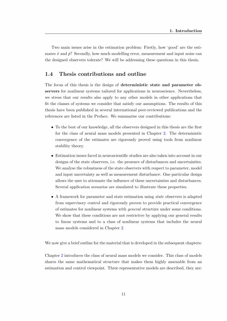
2.3 Detailed block diagram of the Wendling et al. model. Reproduced from
Figure 4 in [155]. . . . . . . . . . . . . . . . . . . . . . . . . . . . . . . 19
2.4 Functional relationship between neural populations for the model by
Jansen and Rit. . . . . . . . . . . . . . . . . . . . . . . . . . . . . . . . 21
2.5 Detailed block diagram of the Jansen and Rit model. . . . . . . . . . . 21
2.6 Functional relationship between neural populations for the model by
Stam et. al.. . . . . . . . . . . . . . . . . . . . . . . . . . . . . . . . . . 21
2.7 Detailed block diagram of the Stam et. al. model. . . . . . . . . . . . . 22
2.8 State observer setup . . . . . . . . . . . . . . . . . . . . . . . . . . . . . 29
2.9 Circle criterion observer: error system . . . . . . . . . . . . . . . . . . . 32
3.1 Model and observer setup under relaxed assumptions. . . . . . . . . . . 39
3.2 Error norm |x(t)| for a selection of k and l. . . . . . . . . . . . . . . . . 41
x

LIST OF FIGURES
3.3 Membrane potential xi1 (grey solid line) and estimated membrane po-
tential contribution xi1 (red solid line: l = k = 0, black dashed line:
k = 0.1, l = −0.5) under the ideal scenario (Assumptions 1 to 4). . . . 42
3.4 True membrane potential contribution xi1 (grey solid line) and estimated
membrane potential contribution xi1 (red solid line: l = k = 0, black
dashed line: k = 0.1, l = −0.5) under the practical scenario (Assump-
tions 5 to 8). . . . . . . . . . . . . . . . . . . . . . . . . . . . . . . . . . 44
3.5 Relative state estimation error |xi−xi|max(xi)−min(xi)
for i ∈ {1, . . . , 7} under
the practical scenario (Assumptions 5 to 8) for the estimator (grey solid
line) and the observer with k = 0.1, l = −0.5 (black dashed line). . . . 45
3.6 Norm of state estimation error |x| for the estimator (grey solid line)
and the observer with k = 0.1, l = −0.5 (black dashed line) under
Assumptions 1, 3, 4 and 6. . . . . . . . . . . . . . . . . . . . . . . . . . 46
3.7 Absolute state estimation error |xi−xi|max(xi)−min(xi)
for i ∈ {1, . . . , 7} for the
estimator (grey solid line) and the observer with k = 0.1, l = −0.5 (black
dashed line) under Assumptions 1, 3, 4 and 6. . . . . . . . . . . . . . . 47
3.8 True membrane potential contribution xi1 (grey solid line) and estimated
membrane potential contribution xi1 (red solid line: k = l = 0, black
dashed line: k = 0.1, l = −0.5) under Assumptions 1, 3, 4 and 6. . . . . 48
4.1 Absolute observation error relative to the amplitude of the signal, |xi||max(xi)−min(xi)| ,
for i ∈ {1, . . . , 4}. . . . . . . . . . . . . . . . . . . . . . . . . . . . . . . . 57
4.2 Estimated states x converge to a neighbourhood of the true states x.
Legend: Observer A (grey), Observer B (red) and Model (black). . . . 61
4.3 Parameter and state estimation . . . . . . . . . . . . . . . . . . . . . . . 63
5.1 n−interconnected models, where i ∈ {2, . . . , n− 1}. . . . . . . . . . . . . 67
6.1 Supervisory observer. . . . . . . . . . . . . . . . . . . . . . . . . . . . . 75
6.2 Sampling of the parameter set Θ ⊂ R2. Dots represent the selected
parameter pi. . . . . . . . . . . . . . . . . . . . . . . . . . . . . . . . . 76
6.3 Simulation results. . . . . . . . . . . . . . . . . . . . . . . . . . . . . . . 87
7.1 Proposed adaptive controller design for seizure abatement . . . . . . . . 93
xi

List of Notations
R The set of real numbers.
R≥0 (>0) The set of non-negative (strictly positive) real numbers.
Rn×m The space of real matrices with dimensions n×m.
(a, b) A vector
a
b
, for all a ∈ Rna and b ∈ Rnb .
diag The matrix
A1 0 . . . 0
0 . . ....
... . . . 0
0 . . . 0 An
, where Ai for
i ∈ {1, . . . , n} are m × m matrices, is denoted asdiag(A1, A2, . . . , An).
λmax(P ) (λmin(P )) The maximum (minimum) eigenvalue of a real, symmetricmatrix P .
? The symmetric block component of a symmetric matrix.
I The identity matrix.
xii

List of Notations
|f(t)| The vector norm of f at each time t.
‖f(t)‖2 The L2 norm of f .
dae The smallest integer larger than or equal to a ∈ R.
η ∈ N(µ, σ2) A signal η ∈ R that is drawn from a Gaussian distribution withmean µ ∈ R and variance σ2 ∈ R.
Br The closed ball centered at 0 for some r > 0 is denoted by Br :={s ∈ Rn : |x| ≤ r}.
L∞ The set of functions f : R → Rn, for some n ∈ Z, such that forany 0 ≤ t1 ≤ t2 ≤ ∞ there exists r ≥ 0 so that ‖f‖[t1,t2] :=supτ∈[t1,t2] |f(τ)| ≤ r.
M∆ The set of piecewise continuous functions from [0,∞) to B∆, forany ∆ > 0.
x[t1,t2] For a signal x : R≥0 → Rn, x[t1,t2] is the signal x(t) considered onthe interval t ∈ [t1, t2].
(·)− The left-limit operator.
K A continuous function α : R≥0 → R≥0 is said to be a class K
function, if it is strictly increasing and α(0) = 0.
KL A continuous function β : R≥0 × R≥0 → R≥0 is said to be a classKL function, if, for each fixed s, the mapping β(r, s) is a classK function with respect to r and for each fixed r, the mappingβ(r, s) is decreasing with respect to s and β(r, s)→ 0 as s→∞.
xiii

Chapter 1
Introduction
1.1 Motivation and scope
Approximately 50 million individuals in the world have fits or convulsions, known
as seizures caused by neurological disorders such as epilepsy and Parkinson’s dis-
ease [5]. These individuals face the uncertainty of uncontrolled seizures that restricts
their daily activities, such as swimming, cooking and driving. In some parts of the
world, they face social stigma and exclusion that ranges from misunderstanding, dis-
advantages in employment to serious consequences brought on by legislation. In fact,
up till 1956, 18 states in the United States of America provided eugenic sterilisation
of epileptic patients [3]. The number of individuals affected by epilepsy is even higher,
at around 200 million when taking into account the family members and friends of
the patient [4]. The cost of epilepsy is therefore not only physical, but also social and
psychological.
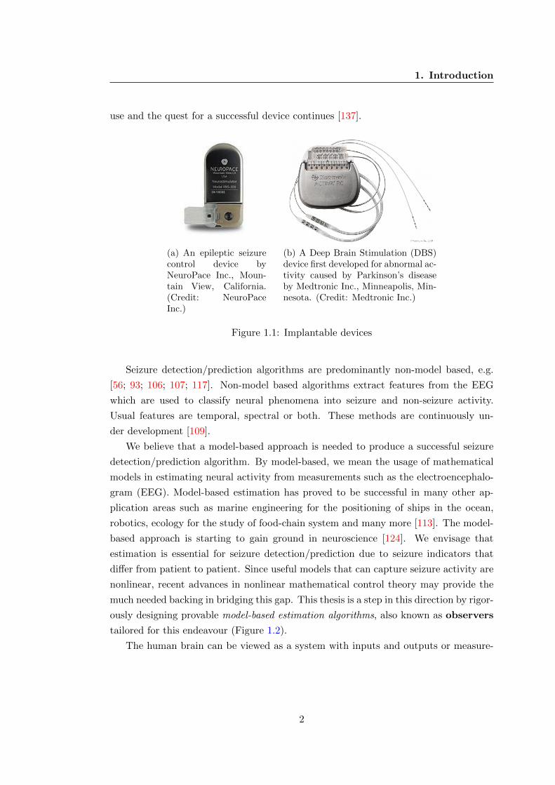
The goal of epilepsy treatment is prevention rather than cure. Fortunately, 70 %
of patients can become seizure free with proper medication. The remainder require
resective surgery or implantable devices for seizure control. Figure 1.1 shows some
implantable devices which have been approved for clinical research only in the United
States [1; 2]. The Deep Brain Stimulation (DBS) device by Medtronic Inc. is still
undergoing clinical trial [1]. Some of these devices monitor electrical brain activity in
a localised region for seizure related activity and delivers controlled electrical pulses to
the region believed to be the seizure foci. The algorithm that monitors brain activity
for abnormality is known in the literature as a seizure detection/prediction algorithm
and the measurement of electrical activity is the electroencephalogram (EEG). The
high false positive rates of these algorithms render these devices undesirable for clinical
1
1. Introduction
use and the quest for a successful device continues [137].
(a) An epileptic seizurecontrol device byNeuroPace Inc., Moun-tain View, California.(Credit: NeuroPaceInc.)
(b) A Deep Brain Stimulation (DBS)device first developed for abnormal ac-tivity caused by Parkinson’s diseaseby Medtronic Inc., Minneapolis, Min-nesota. (Credit: Medtronic Inc.)
Figure 1.1: Implantable devices
Seizure detection/prediction algorithms are predominantly non-model based, e.g.
[56; 93; 106; 107; 117]. Non-model based algorithms extract features from the EEG
which are used to classify neural phenomena into seizure and non-seizure activity.
Usual features are temporal, spectral or both. These methods are continuously un-
der development [109].
We believe that a model-based approach is needed to produce a successful seizure
detection/prediction algorithm. By model-based, we mean the usage of mathematical
models in estimating neural activity from measurements such as the electroencephalo-
gram (EEG). Model-based estimation has proved to be successful in many other ap-
plication areas such as marine engineering for the positioning of ships in the ocean,
robotics, ecology for the study of food-chain system and many more [113]. The model-
based approach is starting to gain ground in neuroscience [124]. We envisage that
estimation is essential for seizure detection/prediction due to seizure indicators that
differ from patient to patient. Since useful models that can capture seizure activity are
nonlinear, recent advances in nonlinear mathematical control theory may provide the
much needed backing in bridging this gap. This thesis is a step in this direction by rigor-
ously designing provable model-based estimation algorithms, also known as observers
tailored for this endeavour (Figure 1.2).
The human brain can be viewed as a system with inputs and outputs or measure-
2

1. Introduction
(1)
(3)
Human brain
Output/ measurements
Measurement module
Sensors/ electrodes
Observer
Estimated neural activity
Input
Figure 1.2: Model-based estimation of neural activity (observers)
ments. Examples of measurements include the electroencephalogram (EEG), functional
magnetic resonance imaging (fMRI) and magnetoencephalogram (MEG), to name a
few. We focus on using the EEG as a measurement due to its cost-effectiveness and
portability such that it is usable in implantable devices. The EEG also has a very high
temporal resolution, in the order of milliseconds, a characteristic that is useful when
detecting high frequency oscillations (HFOs) with frequencies greater than 80 Hz which
are postulated to be an indication of seizure activity [136; 145; 164].
Due to limitations in technology, the EEG is unable to capture all neural activities of
interest. The estimation of unmeasured neural activities is therefore very appealing to
clinicians and neuroscientists. This is due to the possibility of opening up new avenues
for neuroscientific studies, diagnostics and the treatment of neurological disorders via
the development of monitoring or control strategies [69].
One of the primary advantages of estimation lies in reducing the number of sen-
sors/electrodes needed and thereby keeping surgical invasion to a minimum. This is
particularly useful for neurological events such as seizures caused by epilepsy or patho-
logical dynamics of Parkinson’s disease that are generated in deep brain structures such
as the hippocampus and the basal ganglia, respectively. Implanting the smallest re-
quired number of electrodes minimises risks such as infection and haemorrhage as well
as pain that results from implantation.
We provide several examples where an observer is used in the field of neuroscience.
• Neuroscientific studies
The observer serves to enhance neuroscientific studies. The estimation of unmea-
3

1. Introduction
sured neural activities in the setup shown in Figure 1.2 provides neuroscientists
with a basis for generating experimentally provable hypotheses on the underlying
mechanisms that govern a neurological event, such as seizures caused by epilepsy
or Parkinson’s disease. Works by Tokuda et al. in [143], Totoki et al. in [144],
Tyukin et al. in [148] and Mao et al. in [103] perform model-based estimation at
the single neuron level for various neuroscientific purposes. In [150], Ullah and
Schiff performed model-based estimation of the ion concentrations of hippocam-
pal neurons from membrane potential measurements of a neuron to study the
dynamics of ion concentrations during epileptic seizures. Advances in this area
will fuel the development of diagnosing, monitoring and treatment strategies for
neurological diseases as discussed in the sequel.
• A diagnostic system
Experimental studies have provided clinicians and neuroscientists clues to the
presence of certain indicators that suggest the possibility of epilepsy in patients
[136]. An observer would provide estimates of indicators from measurements.
For example, the synaptic gains of the pyramidal neurons, the excitatory and in-
hibitory populations in the CA1 region of the hippocampus have been identified
in [155] as parameters that are related to seizure and non-seizure activity. Clin-
icians may be aided by estimates provided by an observer to diagnose patients
whose parameter estimates consistently belong to the seizure-related range.
• A seizure warning system
This takes the form of using estimates of neural activity from an observer to dis-
cern seizure from non-seizure behaviour by the classifier in the seizure prediction
module (see Figure 1.3). To this end, key features of a seizure need to be known.
Work has been done in identifying parameters of models that are postulated to
be related to seizure activity [153]. We discuss this model in greater detail in
Chapter 2. It is the task of the classifier to raise a red flag when the parameters
fall within the range that have been predetermined to be seizure-related.
• Closed-loop seizure control system
The open-loop warning system can then initiate the administration of drugs or
electric stimulation to abate seizures, which we call a closed-loop control system,
see Figure 1.4. The observer provides estimates of neural activity such that a
control law may be formulated to trigger seizure suppression procedures. We
discuss the design of a control law (see Figure 1.4) in Chapter 7.1, where we
present future directions of this work.
4

1. Introduction
(1)
(3)
Human brain
Output/ measurements
Measurement module
Sensors/ electrodes
Observer
Seizure warning module
Classifier Estimated neural activity
Input
Seizure/ No seizure ?
Figure 1.3: An open-loop warning system
(1)
Input)
Human brain
Output/ measurements
Measurement module
Sensors/ electrodes
Observer
Seizure control module
Control Law
Drug administration/ electrical stimulation
devices
Estimated neural activity
Figure 1.4: Closed-loop seizure control system
The design of observers in the examples mentioned above requires the use of math-
ematical models that appropriately describe the part of the brain concerned and the
measurement used. We briefly discuss our choice of neural models in the following
section.
1.2 Neural model
As mentioned earlier, the EEG is our measurement of choice. Here, we have used the
term EEG as the umbrella term that includes measurements obtained from the scalp
5

1. Introduction
or from the surface of the cortex, sometimes known in the literature as the electrocor-
ticography (ECoG) or intracranial EEG (iEEG). The sensors/electrodes used to obtain
the EEG are implanted on the scalp or surface of the brain. Each sensor provides a
single channel of EEG which is proportional to the electrical discharges of a population
of neurons in a localised volume perpendicular to the surface [115]. This volume of the
brain is known as a cortical column [111, Chapter 7], see Figure 1.5.
(1)
(3)
Human brain
Output, y Input, u
A cortical column
Figure 1.5: A cortical column. (Diagram credit: iStockphoto/Guido Vrola andhttp://www.mada.org.il)
Within a cortical column, the neurons may be categorised by function into inhibitory
and excitatory neurons. They can be pyramidal and basket cells in the hippocampus
or pyramidal cells and thalamic interneurons in the cortico-thalamic system [127]. In
1973, Wilson and Cowan suggested a model for the interaction between inhibitory and
excitatory populations of neurons in [156]. This model forms the basis of many models,
including the neural mass models which we will discuss in greater detail in Chapter 2.
We view each cortical column as a dynamical system Σ (see Figure 1.6), with
measurements or outputs y and inputs u. Examples of an output from a cortical
column model are the average electrical activity of neural populations in the cortical
column or the EEG measurement. Examples of an input are the electrical activity from
neighbouring cortical columns or electrical pulses sent from an implantable device to
suppress seizures. Each system Σ has internal variables or states x and is parameterised
by p∗, which forms a family of parameterised systems (Figure 1.6).
In general, depending on the measurement y considered, the states x may capture
the membrane potential of a neuron (microscopic) or the mean membrane potential of
neuronal populations (mesoscopic) and the parameters p∗ may be the neural membrane
6

1. Introduction
(1)
(3)
Human brain A cortical column
Output, y Input, u
uModel input, Neural model yModel output,
px,
:
Figure 1.6: A cortical column is a system whose dynamics are described by a mathe-matical model.
capacitive current (microscopic) or the synaptic gain of populations (mesoscopic). The
states are physiologically relevant and often unmeasurable by conventional means. The
parameters p∗ are identified to vary as a result of different brain phenomena and hence
usually resides in a known, compact set Θ. For instance, in the case of a model of
epileptic activity in the hippocampus [153], the synaptic gains of the neuronal popula-
tions were identified to be the parameters that change when the brain transitions from
normal to epileptic activity. Hence, the possibility of detecting such changes and to
then develop seizure control strategies to mitigate seizures form great motivation for
the estimation of states x and parameters p∗.
In this thesis, our measurement of choice is the EEG, which is of the mesocopic
scale. Hence, we consider cortical column models that are lumped-parameter models,
also known in the literature as neural mass models, a term coined in [39]. These models
have the added advantage of being able to capture the desired neural phenomenon such
as seizures, while still being of a low enough dimension to be useful in the estimation
and control theoretic sense. This class of systems is represented by ordinary differential
7

1. Introduction
equations and they can be written in state space form as follows:
Σ : x = f(x, u, p∗)
y = h(x, p∗), (1.1)
where the state is x ∈ Rnx , the input is u ∈ Rnu , the parameter is p∗ ∈ Θ ⊂ Rnp ,measurement/output is y ∈ Rny and nx, nu, np and ny are positive integers. Examples
of commonly used neural mass models considered in this thesis are: models for the
generation of alpha rhythms by Jansen and Rit as well as Stam et. al., respectively
in [74; 138] and a model of epileptic activity in the hippocampus by Wendling et. al.
in [155]. These models were based on the seminal work by Wilson and Cowan [156],
Freeman [50] and Lopes da Silva et. al. [99; 100]. We describe these models in greater
detail in Chapter 2.
1.3 The estimation problem
The objective is to estimate the states x and parameters p∗ of the model Σ. The dy-
namical system that computes these estimates is known as an ‘observer ’ or ‘estimator ’
or ‘filter ’ [12; 23]. In this thesis, we will use the term ‘observer’. When the parameter
p∗ is known, we design a state observer to reconstruct the states x of the model Σ.
The observer Σo takes in the available information (the input u and measurement y)
to provide state estimates x. When the parameter p∗ is unknown, Σo is called a state
and parameter observer, which provides estimates of both states x and parameters
p. Figure 1.7 illustrates this setup.
The task of observer design can be approached in two ways: stochastic or determin-
istic. The stochastic approach to estimation is more popularly known in the literature as
‘filtering’ and the system is modelled by stochastic differential/difference equations [75].
Classical, statistical methods such as least-squares, maximum-likelihood and minimum
variance estimation were first applied to linear filtering problems and later extended
to nonlinear cases [83]. A popular point of view is Bayesian-based, i.e. the estimate of
the state can be constructed from the conditional probability density function of the
state, given the available measurements. See [75] for a unified treatment of bayesian-
based linear and nonlinear filtering. Popular stochastic observers include the Kalman
filter and its variants1. These filters are used in many applications, including neuro-
1The Kalman filter can also be formulated deterministically, where its design is reducibleby duality to a linear quadratic optimal control problem [132, Section 8.3].
8

1. Introduction
uModel input, yModel output,
Observer
xState estimate,
Neural model px,
:
:o
pParameter estimate,
Figure 1.7: Observer setup
science [51; 52; 125; 150]. One popular usage of filters in neuroscience is a framework
known as Dynamic Causal Modelling [37; 88; 140], where estimates from the filters are
used to choose the best model that describes the measurements under some conditions.
Stochastic methods provide convergence of estimates with some probability. In other
words, the convergence of the estimates to the true values is not guaranteed for every
trajectory.
On the other hand, the deterministic approach guarantees convergence of estimates.
For the simpler problem of state estimation only, the case for linear systems is com-
pletely solved in the form of a Luenberger observer [101] and the deterministic Kalman
and Bucy filter [78]. This is not the case for nonlinear systems, where no general
solution exists. The design of nonlinear observers is done on a ‘case-by-case’ basis,
which is reliant on the mathematical structure of the model. Hence, it makes sense
to consider a class of systems that share the same mathematical structure and an
observer is designed for that class of systems. Due to the widespread applicability
of nonlinear observers, nonlinear state observer design has been extensively studied
[6; 7; 13; 15; 16; 17; 18; 19; 23; 26; 27; 28; 29; 40; 43; 44; 45; 47; 48; 53; 54; 55; 59; 60;
61; 70; 81; 82; 84; 87; 90; 91; 94; 97; 101; 102; 104; 108; 113; 119; 120; 121; 123; 126;
128; 129; 130; 142; 146; 147; 157; 158; 159; 161; 163]. Deterministic state observers can
generally be categorised into observers for special classes of nonlinearities (e.g. Lips-
9

1. Introduction
chitz nonlinearities [54; 121], monotone nonlinearities [16; 158]) and high gain observers
[13; 87].
We contribute to this body of work with the design of two state observers in Chap-
ters 3 and 4 for a class of nonlinear systems which includes some of the neural models
introduced earlier: a Luenberger-like observer and a robust form of the circle criterion
observers, first introduced in [16]. The existence of a circle criterion observer is based
on the feasibility of a linear matrix inequality (LMI). Existing circle criterion observers
in [16; 17; 45; 158] do not yield LMIs that are feasible for the neural mass models we
consider. Hence, we combined several ideas from these papers including considering
globally Lipschitz nonlinearities and introducing a multiplier to obtain LMIs that are
feasible for our examples. We further improved the design by allowing the user to
specify attenuation factors towards noise.
Similarly for the case of parameter and state estimation. One common approach is
to augment the state vector with the parameters and employ a state observer to estimate
the augmented vector such that we obtain both state and parameter estimates. This
approach is not conducive even for the case of linear systems because doing so may turn
the augmented system highly nonlinear, where the synthesis of a nonlinear observer is
difficult.
An alternative is the design of adaptive observers [20; 22; 26; 32; 46; 57; 89; 104; 105;
122; 139; 149; 158; 160; 161]. An adaptive observer may be viewed as a state observer
with an adaptive law that provides parameter estimates jointly to obtain state esti-
mates. We will take this approach in Chapter 5 where we design an adaptive observer
for a class of nonlinear systems which includes the interesting case of interconnected
neural mass models. This adaptive observer drew inspiration from the design in [46]
which combines the high gain idea used in state observers [13; 87] with an adaptive
observer design for linear time varying systems by Zhang and Clavel in [162].
Another approach uses the multiple-model architecture (see [9] and references there-
in for an overview). This architecture employs a bank of state observers, where each
observer is designed for a particular nominal parameter value chosen from a known set,
to provide state and parameter estimates under some scheme. It has traditionally been
pursued using stochastic methods [12, Section 8.4] and has recently been studied in the
deterministic sense [10], [11]. Encouraged by recent results in supervisory control (see
[64; 152] for linear systems and [21] for nonlinear systems), which uses the multiple
model architecture for stabilisation, we adapted it for estimation purposes in Chapter
6. We call this adapted setup, a supervisory observer and guarantee the convergence
of states and parameter estimates in the deterministic sense under certain conditions.
10
1. Introduction
Two main issues arise in the estimation problem: Firstly, how ‘good’ are the esti-
mates x and p? Secondly, how much modelling error, measurement and input noise can
the designed observers tolerate? We will be addressing these questions in this thesis.
1.4 Thesis contributions and outline
The focus of this thesis is the design of deterministic state and parameter ob-
servers for nonlinear systems tailored for applications in neuroscience. Nevertheless,
we stress that our results also apply to any other models in other applications that
fit the classes of systems we consider that satisfy our assumptions. The results of this
thesis have been published in several international peer-reviewed publications and the
references are listed in the Preface. We summarise our contributions:
• To the best of our knowledge, all the observers designed in this thesis are the first
for the class of neural mass models presented in Chapter 2. The deterministic
convergence of the estimates are rigorously proved using tools from nonlinear
stability theory.
• Estimation issues faced in neuroscientific studies are also taken into account in our
designs of the state observers, i.e. the presence of disturbances and uncertainties.
We analyse the robustness of the state observers with respect to parameter, model
and input uncertainty as well as measurement disturbance. One particular design
allows the user to attenuate the influence of these uncertainties and disturbances.
Several application scenarios are simulated to illustrate these properties.
• A framework for parameter and state estimation using state observers is adapted
from supervisory control and rigorously proven to provide practical convergence
of estimates for nonlinear systems with general structure under some conditions.
We show that these conditions are not restrictive by applying our general results
to linear systems and to a class of nonlinear systems that includes the neural
mass models considered in Chapter 2.
We now give a brief outline for the material that is developed in the subsequent chapters:
Chapter 2 introduces the class of neural mass models we consider. This class of models
shares the same mathematical structure that makes them highly amenable from an
estimation and control viewpoint. Three representative models are described, they are:
11

1. Introduction
(i) a model by Stam et. al. in [138] that described alpha rhythms seen in the EEG, (ii)
a model by Jansen and Rit in [74] that describes the generation of alpha rhythms in the
cerebral cortex and (iii) a model by Wendling et. al. in [153] that describes epileptic
activity in the hippocampus. We will provide a brief overview of the physiological in-
terpretation of these models and then present them in state space form, which is most
convenient for observer design.
This thesis can be read in two parts: Part I (Chapters 3-4): State estimation and
Part II (Chapters 5-6): Parameter and state estimation.
Part I: State estimation
Chapter 3 presents a nonlinear observer that is designed for this class of neural mass
models. Some highly desirable features of these models allow us to design an estimator
that has a state error system with a cascaded structure. This allows us to apply the
interesting result of ISS for cascaded systems in stability analysis [86, Lemma 4.7]. We
will also show that the designed observer has desirable robustness properties.
Chapter 4 introduces a robust circle criterion observer that we have designed. This
observer takes into account two main robustness issues encountered in neuroscientific
studies, that is input uncertainty and measurement noise. We allow the user to specify
attenuation factors towards these undesirables and should a derived LMI be solvable,
a robust circle criterion observer can be obtained.
The success of state estimation and the robustness of the designed observers toward
small perturbations in parameters motivated the next step towards achieving our goal,
that is parameter and state estimation in the following part.
Part II: Parameter and state estimation
Chapter 5 presents an adaptive observer for the class of neural mass models we con-
sider, which can be written as a linear part and a triangular nonlinear part that is
linearly parameterised. We exploited this structure to design an adaptive observer that
is applicable to a subset of the class of models considered and most interestingly, inter-
connected models in this subset.
Chapter 6 proposes using a multi-observer to provide state and parameter estimates
for general nonlinear systems under the supervisory framework. We call this setup the
12

1. Introduction
supervisory observer. The results obtained are applicable to general nonlinear systems
and we show that our main results can be applied to the class of neural mass models
considered in Chapter 2.
Finally, Chapter 7 concludes this thesis with some discussion for future work. Ap-
pendix A serves as a primer on the stability tools used in observer design and the
analysis of systems in this thesis. Appendix B contains all mathematical proofs of re-
sults and lastly, Appendix C lists standard values of the constants used in the considered
class of neural mass models.
13

Chapter 2
Neural models
We first provide a definition of the basic neurophysiological terminology used in
the literature and in this thesis. The intention is not to be comprehensive, but
serves to set the stage for the types of neural models considered for observer design and
the physiological meaning of the states and parameters estimated. We then introduce
the class of neural models considered in this thesis and write these models in state
space form in state coordinates that are convenient for observer design.
2.1 Basic neurophysiological and electroencephalographi-
cal terminology
The respective definitions of the neurophysiologically related terminology below can be
found in [38; 79; 127] and electroencephalography related terminology can be found in
[115]. Here, we present a glossary of basic terms used.
• Neurons are cells that are found in the brain. There is an estimate of more than
1011 neurons in the human brain.
• A neuron consists of a cell body or soma, dendrites and axon. See Figure 2.1.
• Action potentials or impulses or spikes are generated by neurons and they are the
communication signal between neurons. These signals are received by dendrites,
processed in the soma and the neuron outputs signals to other neurons via its
axon.
• The neuronal response to stimuli is often a sequence of action potentials which
can be characterised through their timing. The firing rate captures the average
14

2. A class of neural mass models
Dendrite
Synapse
Synapse
Axons from other neurons
Dendrite
Dendrite
Cell body (Soma)
AxonOutput
Input
Figure 2.1: A neuron. (Diagram credit: Crystal Chong)
number of spikes (action potentials) in a time interval.
• The synapse is the junction between the dendrite of one neuron and the axon of
another neuron. There are electrical and chemical synapses.
• Electrical synapses are direct, electrically conductive junctions.
• Chemical synapses transmit signals from the pre-synaptic cells to the post-synaptic
cells that are separated by the synaptic cleft. When an action potential is re-
ceived by an axon, chemical and electrical reactions are triggered which causes
the release of neurotransmitters into the synaptic cleft. They diffuse across the
synaptic cleft and react with the transmitter-gated ion channels (i.e. receptors)
on the postsynaptic cell, causing a change in the postsynaptic potential (PSP).
• The postsynaptic potential (PSP) is in the milli-Volts (mV ) range.
• The synaptic gain or strength of a single synapse is quantified by the gain in
the amplitude of the PSP as a result of a pre-synaptic action potential. The
synaptic gain of a single synapse is proportional to the amount of neurotransmitter
released and the number of postsynaptic receptors. The total synaptic gain from
the presynaptic cell to the postsynaptic cell is proportional to the number of
connections from the presynaptic cell to the postsynaptic cell.
15

2. A class of neural mass models
• A neuron can either be excitatory or inhibitory. An excitatory neuron transmits
action potentials to a receiving neuron causing an increase in PSP in the receiving
neuron. This event is known as depolarisation and is amenable to the generation
of action potentials. On the other hand, a neuron that causes a decrease in PSP
or hyperpolarisation is an inhibitory neuron. This decreases the likelihood of
action potential generation. Excitation and inhibition are mediated by multiple
neurotransmitters. An example of a major neurotransmitter is the γ-aminobutyric
acid (GABA), which is commonly found in the hippocampus.
• The hippocampus is one of the most well-studied parts of the mammalian brain.
Most epileptic patients have seizures that involve the hippocampus. The principal
neurons in the hippocampus are the pyramidal neurons. Depending on their size
and appearance, the pyramidal cell layer is divided into three regions labelled
CA1, CA2 and CA3. A member of the class of neural mass models considered
(the model by Wendling et. al. in [155]) models the CA1 region.
• Intrinsic neurons or interneurons are a type of neuron with a locally restricted
axon plexus that lack spines and release γ-aminobutyric acid (GABA). There are
two types of GABA dynamics in the CA1 pyramidal neurons: a fast response
near the soma and a slow response near the dendrites. These populations are
included in the model by Wendling et. al. in [155].
• A neural population refers to a group of neurons characterised by location (e.g.
cortex, hippocampus) or by type (e.g. excitatory, inhibitory, pyramidal). Com-
mon nomenclatures include a cortical column, excitatory population or inhibitory
population. The mean PSP or membrane potential of a neural population is the
average potential of all the neurons in that population.
• A cortical column is a group of neurons in the cortex that reside in a column of
300−500µm in diameter perpendicular to the surface of the cortex [111, Chapter
7].
• The electroencephalogram (EEG) measures the electrical activity of neural pop-
ulations [115]. It is said to reflect the mean PSP or mean membrane potential
of neural populations. The sensors used to measure EEG are electrodes that can
be placed on the scalp and the measurement is known as ‘scalp EEG ’ or near the
surface of the brain to measure ‘intracranial EEG (I-EEG)’, ‘electrocorticography
(ECoG)’ or ‘subdural EEG (SD-EEG)’. Often in epilepsy studies, depth electrodes
16

2. A class of neural mass models
are inserted in brain structures such as the hippocampus to capture the focus of
the seizure, that is otherwise poorly localised in the scalp EEG.
• Alpha rhythms are oscillations of 9− 11 Hz observed in the EEG. These patterns
are often recorded when the subject’s eyes are closed in a relaxed, awake state.
2.2 Neural models
Mathematical models in neuroscience can be largely classified into comprehensive mod-
els and heuristic models. Comprehensive models are constructed by taking into account
all known neurophysiological facts and data. An example is the Nobel-prize winning
model of the initiation and propagation of action potentials in a single neuron by
Hodgkin and Huxley [68]. As the facts and data considered increases (e.g. modelling
a population of neurons as opposed to a single neuron), so does the complexity of the
model increase. Since neuroscience is a largely evolving field, we are still far from
painting a complete picture even when considering all known facts. Moreover, the high
complexity of these models often makes them not amenable for analysis. Therefore, this
motivates the construction of heuristic models that are less complex, but still capture
the essential features of a neurological event.
Heuristic models are constructed by including assumed relevant facts to describe a
neurological phenomenon of interest via a dynamical system. Since there is no universal
agreement over which facts are relevant to a particular phenomenon, the literature for
such models is large (see [39] for a review) and more work needs to be done to integrate
theoretical neuroscience with experimental work to assess the realism of these models.
Neural modelling of this type is therefore more of an art. As our measurement of
choice is the electroencephalogram (EEG), which best measures the behaviour of a
population of neurons, we consider models that capture the temporal dynamics of
neural populations. These are coined in [39] as neural mass models and are governed
by ordinary differential equations.
Our motivation lies in anticipating the occurrence of epileptic seizures from the
EEG, which is a phenomenon captured by a member of a class of neural mass models
that share the same mathematical structure. Other members of this class describe
neurological events that include but are not limited to the generation of alpha rhythms
and the generation of evoked potentials due to a visual input in the cerebral cortex.
We describe them in greater detail in Section 2.3.
17

2. A class of neural mass models
2.3 A class of neural mass models
In this section, we present the class of neural mass models we consider, which includes
the following models that share the same mathematical structure in their dynamics:
(i) The model by Wendling et. al. in [155] that captures epileptic activity in the
hippocampus, (ii) The model by Jansen and Rit in [74] on the generation of evoked
potentials due to visual stimulation, and (iii) The model by Stam et. al. in [138] for the
generation of alpha rhythms. These models have their origins in cortical column models
by Wilson and Cowan [156], Freeman [50] and Lopes da Silva et. al. [99; 100]. In the
proceeding sections, the class of neural mass models are presented with decreasing level
of complexity. The functional connections between the neural populations for each of
the models and their corresponding more detailed block diagrams are shown in Figure
2.2-2.7.
2.3.1 Neural mass model by Wendling et. al.
Wendling et. al. built upon the Jansen and Rit model described in the Section 2.3.2.
Four neural populations (with one population being a subset of another) are included
in this model as shown in Figure 2.2.
!"#$%&'$()*+,#-./)
0.1&2&3-#")0.3+#.+,#-./)4/(-5)'+.'#&67)8#-9+76-.:)
0.8,3;)u(t)
<,38,3;)y(t) 4==>:)
?) ?)
@)
!"#$%&'(%))'(*+"&'
0.1&2&3-#")0.3+#.+,#-./)4A$/3)/-%$67)8#-9+76-.:)
@)
@)
BC) BD)
BE)
BF)
BG)
BH)
BI)
Figure 2.2: Functional relationship between neural populations for the model byWendling et. al..
The populations are the pyramidal neurons, the excitatory population (included in
the pyramidal neurons), the slow and fast inhibitory populations. The fast somatic
projection of the inhibitory interneurons is introduced in this model because it is hy-
pothesised to play a role in the fast oscillatory pattern seen in the EEG at the onset of
an epileptic seizure. Wendling et. al. identified three parameters, namely the synaptic
gains of the excitatory, slow inhibitory and fast inhibitory interneurons to result in the
18
2. A class of neural mass models
model producing EEG patterns that are known to be related to neurological events,
from normal background activity to epileptic seizures. This provides great motivation
for estimating these parameters.
Figure 2.3 describes the interaction between populations of neurons in greater detail,
which consists of postsynaptic membrane potential (PSP) kernels he, hi and hg, sigmoid
functions S : R→ R and connectivity constants C1 to C7.
C1 C2
C3
C4
C5
)(the
)(the
)(thi
)(thg
)(the
)(the
)(thi
].[ !!!S
11x!"
#"#"
#" !"
$%&"'(")$)"
!"!"
21x31x
71x
61x
51x
41x
].[ !!!S
].[ !!!S
].[ !!!S
)*+,&-.,/"01%+'02"
C6
)(ty!"#$%&"'()'(*&)(tu!"#$%&+,)'(*&
31%+,/"&,22"&'.1/"
C7"
405-6-7'+*"-071+01%+'02"82/'9".10.+-:;"<+'=1;:'0>"
405-6-7'+*"-071+01%+'02"8(,27"2'&,:;"<+'=1;:'0>"
Figure 2.3: Detailed block diagram of the Wendling et al. model. Reproduced fromFigure 4 in [155].
The firing rate of the afferent population is converted into an excitatory, slow or
fast inhibitory postsynaptic membrane potential via the following kernels, for t ≥ 0:
• The excitatory population:
he(t) = θAat exp(−at). (2.1)
• The slow inhibitory population:
hi(t) = θBbt exp(−bt). (2.2)
• The fast inhibitory population:
hg(t) = θGgt exp(−gt). (2.3)
Parameters θA, θB and θG in (2.1)-(2.3) correspond to the synaptic gains of the excita-
tory, slow and fast inhibitory populations respectively. These parameters characterise
19

2. A class of neural mass models
the observed pattern in the EEG. For example, the values of θA, θB and θG that dis-
tinguish between seizure and non-seizure activities have been identified in [155].
Internal variables x11, . . . , x71 are introduced as shown in Figure 2.3. They describe
the membrane potential contribution from one population to another. For example,
referring to Figure 2.3, the mean membrane potential of the pyramidal neurons is
x11−x21−x31, which reflects the membrane potential contribution from the excitatory,
slow and fast inhibitory populations, respectively. The mean membrane potential of a
population is converted into the average firing rate of all the neurons in that population
using a sigmoid function S:
S(z) =α2
1 + exp(− r2(z − V2)
) , for z ∈ R, (2.4)
where α2 is the maximum firing rate of the population, r2 is the slope of the sigmoid
and V2 is the threshold of the population’s mean membrane potential.
The neural populations are connected with connectivity strengths C1 to C7, which
represents the average number of synaptic contacts between the neural populations
concerned.
2.3.2 Neural mass model by Jansen and Rit
The interactions between the pyramidal neurons, excitatory and inhibitory populations
(Figure 2.4) are described in this model to investigate the generation of evoked poten-
tials in the cerebral cortex. A detailed block diagram is provided in Figure 2.5. As this
model was extended upon by Wendling et. al. (whose model is presented in Section
2.3.1), each component of the block diagram: the PSP kernels he and hi and sigmoidal
function S are as described in Section 2.3.1.
2.3.3 Neural mass model by Stam et. al.
The model by Stam et. al. includes an excitatory and inhibitory population (Figure 2.6)
to replicate the alpha rhythms in the EEG. This event is related to the human subject
being in a relaxed state with the eyes closed. Hence, the estimation of the unmeasured
postsynaptic potential (PSP) of neural populations may better our understanding of
the visual pathway while in an idle state.
Figure 2.7 shows a detailed block diagram of the model. This model differs from
the models by Wendling et. al. and Jansen and Rit in the sense that the firing rate
of a population is converted to a postsynaptic potential via different kernels from (2.1)
20

2. A class of neural mass models
!"#$%&%'()*+,%-(,-.(',/*
0)(&1$2&3*4-.(',/*
+,5$6$%'()*+,%-(,-.(',/*
+,7.%8*u(t)
9.%7.%8*y(t) :!!;<*
=*
=* =*
>*
!"#$%&'(%))'(*+"&'
?@*
?A*
?B*
?C*
Figure 2.4: Functional relationship between neural populations for the model by Jansenand Rit.
C1
C3
C4
)(the
)(the
)(the
)(thi
].[ !!!S
11x+"
#"
Sum"of"PSP"
+" +"
21x
51x
41x
].[ !!!S
].[ !!!S
Pyramidal"neurons"
)(tyModel&output,&)(tuModel&input,&
Neural"mass"model"
Inhibitory"interneurons"
Excitatory"interneurons"
C2
Figure 2.5: Detailed block diagram of the Jansen and Rit model.
Excitatory*popula.on*
Inhibitory*Interneurons*
Input,*u(t)
Output,*y(t) (EEG)*
+*
;*
C3*
C4*
Neural'mass'model
Figure 2.6: Functional relationship between neural populations for the model by Stamet. al..
21

2. A class of neural mass models
C3
C4
)(the
)(the
)(thi
11x+"
#"
Sum"of"PSP"
21x
51x
].[ !!!S
].[ !!!S
Excitatory"interneurons"
)(tyModel&output,&)(tuModel&input,&
Neural"mass"model"
Inhibitory"interneurons"
Figure 2.7: Detailed block diagram of the Stam et. al. model.
and (2.2), for t ≥ 0:
• Excitatory population:
he(t) = θA[exp(−a1t)− exp(−a2t)]. (2.5)
• Inhibitory population:
hi(t) = θB[exp(−b1t)− exp(−b2t)]. (2.6)
Also, the sigmoid function that converts the postsynaptic potential to the firing
rate of the population differs from (2.4) for the models by Wendling et al. and Jansen
and Rit, as follows:
S1(z) =
{α1 exp
(r1(z − V1)
)z ≤ V1,
α1
(2− exp
(− r1(z − V1)
))z > V1,
(2.7)
where α1 is the maximum firing rate of the population, r1 is the slope of the sigmoid
and V1 is the threshold of the population’s mean membrane potential.
2.4 Neural mass models in state space form
Our observer design is most conveniently carried out using the state space form of the
neural mass models. However, some of the neural mass models of interest presented
in Section 2.3 were in block diagram form (e.g. Figure 2.3, 2.5 and 2.7) in the given
references [74; 138; 155]. In [74] and [155], state space forms were provided but not in
the convenient state coordinates where the techniques we use for proving convergence
22

2. A class of neural mass models
of estimates can be applied. Therefore, we illustrate how this can be done for the model
by Wendling et al., whose detailed block diagram can be found in Figure 2.3. The other
models considered are special cases of the model by Wendling et al. and hence, can
easily be obtained from the derivation below.
We will show that all neural mass models from Section 2.3 can be written in the
following state space form:
x = Ax+G(p?)γ(Hx) + σ(u,Cx, p?), (2.8)
and the output of the model is:
y = Cx, (2.9)
where the state vector is x ∈ Rnx , input is u ∈ R, output/EEG measurement is y ∈ R,
parameter vector is p? ∈ Rnp , G : Rnp → Rnx×m, nonlinearity γ = (γ1, . . . , γm) with
γi : R→ R for i ∈ {1, . . . ,m} and nonlinearity σ = (σ1, . . . , σn) with σi : R×R×Rm →R for i ∈ {1, . . . , n}. The number of states nx, number of parameters np and number
of scalar nonlinear functions m differs for each model. These are defined in Sections
2.4.2-2.4.4.
2.4.1 Physiological interpretation
Physiologically, the first term in (2.8) implements the postsynaptic potential (PSP)
kernels from (2.1), (2.2) and (2.3). This is effectively a convolution of the pre-synaptic
firing rates arriving from other populations with the appropriate PSP response func-
tions. These firing rates are modelled in the second and third term in (2.8) that
incorporates the sigmoid firing rate function of the depolarisation of contributing pop-
ulations. The second term, G(p)γ(Hx), reflects the influence of all states except the
membrane potential of pyramidal population Cx. While the third term, σ(u,Cx, p),
reflects the influence of the mean membrane potential of the pyramidal cells Cx and
the exogenous input u. Neurobiologically, G(p)γ(Hx) + σ(u,Cx, p) correspond to the
effects of intrinsic and extrinsic connections. In other words, when coupling different
neural mass models, one has to consider the (intrinsic) influence of populations within
a neural mass model and (extrinsic) contributions from other neural mass models. The
extrinsic contributions are usually mediated through pyramidal cell populations.
In the following sections, we present the state space form for each model for ease
of observer design. Detailed derivations are first shown for the model by Wendling et
23

2. A class of neural mass models
al., as it is the most complex model and then the subtle differences in derivations are
described for the other models.
2.4.2 State space form for the model by Wendling et al.
We write the Wendling et al. model in state space form by introducing the state vari-
ables xi1 for i ∈ {1, . . . , 7} as the membrane potential contribution from one population
to another and xi2 for i ∈ {1, . . . , 7} as its derivative. The states xi1 are introduced
at the outputs of all the impulse responses he, hi and hg blocks as shown in Figure
2.3. Recalling that the Laplace transform of the impulse responses he, hi and hg (as
described by (2.1), (2.2) and (2.3)) are second-order transfer functions, by performing
the inverse Laplace transform, each transfer function is represented by a second-order
ordinary differential equation (ODE). We show this transformation for he from (2.1)
as an example. Let the input to the he block be u and output be y. We denote the
Laplace transform of signal v as L(v). Hence, the Laplace transform of he with zero
initial conditions is:
L(he(t)) = L(θAat exp(−at)) =θAa
(s+ a)2. (2.10)
Recalling that L(he) = L(y)L(u) , we obtain:
L(y)s2 + 2aL(y)s+ a2L(y) = θAaL(u). (2.11)
By taking the inverse Laplace transform, we obtain a second-order ODE as follows:
¨y + 2a ˙y + a2y = θAau. (2.12)
The xi2 states are defined as xi2 = xi1 for i ∈ {1, . . . , 7} to rewrite the second-order
ODEs as two first-order ODEs for each impulse response block.
We illustrate this for the he(t) block in the fast inhibitory population, then the
output of that block is y = x51 and the input is u = C3S(x11 − x21 − x31). Taking
x52 = x51, (2.12) can be written as two first-order ODE as follows:
x51 = x52
x52 = −2ax52 − a2x51 + θAaC3S(x11 − x21 − x31).
Hence, each impulse response he, hi and hg will each introduce a first-order ODE
24

2. A class of neural mass models
in the following general state space form by taking xi = (xi1, xi2) for i ∈ {1, . . . , 7}:
xi = Aixi + (0, ϑiS(µi) + ϕi) , (2.13)
where µi is the input to the respective sigmoid functions,
Ai =
[0 1
−ki1ki2 −(ki1 + ki2)
], for i = {1, . . . , 7} with k11 = k41 = k51 = k61 = a,
k12 = k42 = k52 = k62 = a, k21 = k71 = b, k22 = k72 = b, k31 = g and k32 = g. ϑi
and ϕi are defined as such ϑ1 = θAaC2, ϑ2 = θBbC4, ϑ3 = θGgC7, ϑ7 = θBbC6, ϑ4 =
ϑ5 = ϑ6 = 0 and ϕ1 = θAau, ϕ2 = ϕ3 = ϕ7 = 0, ϕ4 = θAaC1S(y), ϕ5 = θAaC3S(y),
ϕ6 = θAaC5S(y). Constants a, b and g are strictly positive. S is a sigmoid function
described by (2.4). All constants discussed in this section are summarised in B.12.
The subsystems defined in (2.13) are put together to be written compactly in state
space form (2.8)-(2.9) for ease of observer design.
We take the state vector in (2.8) and (2.9) to be x = (x1, . . . , x7) where xi for
i = {1, . . . , 7} satisfy (2.13). The states x1, x2 and x3 capture the membrane potential
contribution and its derivative of the excitatory, slow and fast inhibitory populations to
the pyramidal neurons, respectively. The states x4, x5 and x6 capture the membrane
potential contribution and its derivative of the pyramidal neurons to the excitatory,
slow and fast inhibitory populations, respectively. The output is y = x11 − x21 − x31.
The specific matrices in (2.8) and (2.9) are denoted as:
• The parameter vector is p? = (θA, θB, θG),
• The matrix A = diag(A1, . . . , A7),
• γ = (S, S, S), where S is defined in (2.4),
• σ = (0, θAau, 0, 0, 0, 0, 0, θAaC1S(y), 0, θAaC3S(y), 0, θAaC5S(y), 0, 0), where S is
described by (2.4),
• C = [ 1 0 −1 0 −1 0 0 0 0 0 0 0 0 0 ],
25

2. A class of neural mass models
• G =
0 0 0
θAaC2 0 0
0 0 0
0 θBbC4 0
0 0 0
0 0 θGgC7
0 0 0
0 0 0
0 0 0
0 0 0
0 0 0
0 0 0
0 0 0
0 θBbC6 0
,
• H =
0 0 0 0 0 0 1 0 0 0 0 0 0 0
0 0 0 0 0 0 0 0 1 0 0 0 0 0
0 0 0 0 0 0 0 0 0 0 1 0 −1 0
.
2.4.3 State space form for the model by Jansen and Rit
We write the model in state space form by taking the state vector in (2.8) to be
x = (x1, x2, x4, x5), where xi for i = {1, 2, 4, 5} satisfy (2.13). States x1 and x2 are
the membrane potential contribution and its derivative of the excitatory and inhibitory
populations to the pyramidal neurons, respectively. States x4 and x5 capture the
membrane potential contribution and its derivative of the pyramidal neurons to the
excitatory and inhibitory populations, respectively. The output is y = x11 − x21. The
specific matrices in (2.8) and (2.9) are denoted as:
• The parameter vector is p? = (θA, θB, C1, C2, C3, C4),
• A = diag(A1, A2, A4, A5),
• γ = (S, S) where S is defined in (2.4),
• σ = (0, θAau, 0, 0, 0, θAaC1S(y), 0, θAaC3S(y)),
• C = [ 1 0 −1 0 0 0 0 0 ],
26

2. A class of neural mass models
• G =
0 0
θAaC2 0
0 0
0 θBbC4
0 0
0 0
0 0
0 0
,
• H =
[0 0 0 0 1 0 0 0
0 0 0 0 0 0 1 0
].
2.4.4 State space form for the model by Stam et al.
The model is written in state space form by taking the state vector in (2.8) as x =
(x1, x2, x5) where xi for i = {1, 2, 5} satisfy (2.13). State x1 = (x11, x12) represents
the mean membrane potential of the excitatory population’s activity to itself and its
derivative, respectively. States x2 = (x21, x22) and x5 = (x51, x52) represent the mean
membrane potential and its derivative of the inhibitory population to the excitatory
population and vice versa, respectively. The output is y = x11 − x21.
As mentioned in Section 2.3.3, the PSP kernels he and hi differ from the ones in the
models by Wendling and Jansen et. al.. Nevertheless, rewriting (2.5)-(2.7) into state
space form does not differ from the derivation presented in Section 2.4. By following
the procedure described in Section 2.4.2, i.e. by taking Laplace transformations of
(2.5) and (2.6) and taking the inverse Laplace transform, the kernels can be written as
second-order ODEs. They can then be rewritten as two first-order ODEs by introducing
extra state variables, xi2 for i ∈ {1, 2, 5}, in a similar fashion as in Section 2.4.2. The
specific matrices in (2.8) are denoted as:
• The parameter vector is p? = (C3, C4),
• A = diag(A1, A2, A5),
• γ = S1 where S is from (2.7),
• σ = (0, θA(a2 − a1)u, 0, 0, 0, θA(a2 − a1)C3S1(y)),
• C = [ 1 0 −1 0 0 0 ],
• G = (0, 0, 0, θB(b2 − b1)C4, 0, 0),
27

2. A class of neural mass models
• H = [ 0 0 0 0 1 0 ].
2.5 Summary
Three examples from a class of neural mass models are presented in this chapter. They
are the models by Wendling et. al., Jansen and Rit as well as Stam et. al. respectively.
A distinct feature of the neural mass models considered in this chapter is that they are
parameterised models, where the parameters dictate the type of output that is known
to represent certain brain activities, such as alpha rhythms in the visual system and
epileptic activity. It is known that the brain transitions into different activities in time,
such as from non-seizure to seizure conditions. Hence, a more accurate representation
would involve assigning dynamics to parameters, where the dynamics are likely to
involve the states. One such model was done by Suffczynski et. al. [141] to explain the
generation of generalised absence seizures, a form of whole-brain epilepsy. We did not
consider such models in this thesis.
The models discussed in this chapter are cortical column models. Cortical columns
are repeated all over cortical brain surfaces, such as in the cerebral cortex or the
hippocampus. Therefore, cortical column models can be used to describe an arbitrary
volume of the brain, a feature useful for describing localised neurological events. Often,
neurological events also have spatial dynamics, such as the spread of seizures from a
foci. These events have dynamics that are governed by partial differential equations and
are known as neural field models [39]. These models are not in the scope of this thesis.
Another way of capturing the spatial activity of a neurological event is to interconnect
the single cortical column models to characterise the phenomenon in a cortical area,
such as the primary visual cortex or even across a larger brain volume. We take this
approach in Chapter 5 where we design an adaptive observer that can estimate the
mean membrane potential (states) as well as the synaptic gains (parameters) of the
neural populations for each of the interconnected single cortical column models.
In Section 2.4 of this chapter, we write each of these example models in a form
that is most amenable for the design of state observers in Part I as well as state and
parameter observers in Part II of this thesis.
28

Part I: State estimation
In this part, the estimation of states under the assumption that the parameter is
known is performed using the setup illustrated in Figure 2.8. The dynamical system
that computes an estimate of the state x of the system Σ is called a state observer.
uModel input, yModel output,
State observer x
State estimate,
Neural model
px,
:
:o
Figure 2.8: State observer setup
As mentioned in the introduction, two important issues need to be addressed in
state observer design, which are also applicable to state and parameter observer design.
Firstly, do the state estimates x (similarly, parameter estimates p) converge to their
true values? Secondly, how do the observers perform in the presence of modelling error,
measurement and input noise?
In response to the first set of questions, recall that the neural model (or system) as
stated in (1.1) in Chapter 1 takes the following form
Σ : x = f(x, u, p∗)
y = h(x, p∗), (2.14)
where the state is x ∈ Rnx , the input is u ∈ Rnu , the parameter is p∗ ∈ Θ ⊂ Rnp ,measurement/output is y ∈ Rny and nx, nu, np and ny are positive integers.
A state observer for the model (2.14) takes the following form
˙x = f(x, u, p∗, y)
y = h(x, p∗), (2.15)
29

Part I: State estimation
where the state estimate is x ∈ Rnx , the input is u ∈ Rnu and the output estimate is
y ∈ Rny . Our task is to design f such that the state estimate converges to its true
value.
To achieve this objective, we consider the state estimation error system (similarly,
the parameter estimation error system. However, we concentrate only on state estima-
tion in this part.). Denoting the state error as x := x−x, we obtain the following state
error system from (2.14) and (2.15):
˙x = f(x+ x, u, p∗, y)− f(x, u, p∗). (2.16)
We define two types of observers based on the convergence properties of their es-
timates via the stability of the equilibrium point of the state estimation error system
(2.16).
Definition 1. If the origin of the state error system (2.16) x = 0 is:
• exponentially stable1, the observer (2.15) is termed exponentially convergent. If
the conditions hold for all x(0) ∈ Rnx, the observer (2.15) is called globally
exponentially convergent.
• asymptotically stable1, the observer (2.15) is termed asymptotically convergent
and if the conditions stated are satisfied for all x(0) ∈ Rnx, the observer (2.15) is
globally asymptotically convergent.
Given general nonlinear systems, the design of convergent observers are reliant on
the specific structures of the systems considered. The simplest case being error systems
that are linear. For example, consider the nonlinear system x = Ax + γ(y), y = Cx,
where γ is a nonlinear function. An observer ˙x = Ax+γ(y)+L(Cx−y) can be designed
and the resulting error system ˙x = (A + LC)x is linear. Given that the pair (A,C) is
detectable, the observer matrix L can be chosen such that the matrix A+LC is Hurwitz,
which ensures that the designed observer is exponentially convergent. In cases where
a general nonlinear system is considered and suppose some coordinate transformation
exists such that the resultant state error is linear, then a convergent observer can also
be achieved [72, Chapter 4.9], [90; 91].
Another well-known nonlinear observer is the high-gain type, which extends the
aforementioned idea of linear error systems by using a high gain to compensate for the
nonlinear part such that the resulting error system is ‘almost’ linear [13; 29; 54; 123].
1see Definition 2 in Appendix A
30

Part I: State estimation
As with all other observer designs for nonlinear systems, the high gain observer is only
applicable to a class of nonlinear systems with special structures. Consider for example
the nonlinear system [23, Chapter 2.2.2]:
x = Ax+ γ(u, x),
y = Cx, (2.17)
where γ is globally Lipschitz, C =[
1 0 . . . 0], A =
0 1 0...
. . .
1
0 . . . 0
and
γ(u, x) =
γ1(x1, u)
γ2(x1, x2, u)...
γn(x, u)
(triangular form).
The high gain observer takes the form ˙x = Ax + γ(u, x) + ∆K(Cx − y), where
∆ = diag(d, d2, . . . , dn), with the parameter d > 0 to be chosen and the observer
matrix K to be designed. By considering a scaled state error, x := ∆−1x, the resulting
scaled error system is ˙x = d(A+KC)x+ ∆−1(γ(u, x)− γ(u, x)). The parameter d > 0
can then be chosen sufficiently large such that the origin of the scaled error system is
exponentially stable [23, Chapter 2.2.2]. Such ideas have also been employed in the
design of adaptive observers [25; 26; 46], of which we will be adapting to suit the class
of neural mass models we consider in Chapter 5.
Two notable drawbacks of the high gain design are that it relies heavily on the global
Lipschitzness and the triangular structure of the nonlinearity γ. The circle criterion
observer introduced by Arcak and Kokotovic [16] removes these restrictions. Consider
now a class of nonlinear systems x = Ax + Gγ(Hx) + σ(y, u) and the proposed circle
criterion observer takes the form ˙x = Ax+Gγ(Hx+K(Cx−y))+L(Cx−y)+σ(y, u).
The error system is viewed as Lure’s system (Figure 2.9) and two restrictions are placed
on the error system in order to satisfy the well-known multi-variable circle criterion [86,
Theorem 7.1]. The two restrictions are that the linear part of the error system H(s)
is strictly positive real (SPR) and the nonlinearity γ is monotonically increasing. The
satisfaction of the SPR condition is implied by the feasibility of a linear matrix in-
equality (LMI). Several relaxations on the system have been performed to obtain a less
conservative LMI, including introducing a multiplier [45] or by considering a globally
Lipschitz nonlinearity γ [17; 158]. For the class of neural mass models considered, the
31

Part I: State estimation
original circle criterion observer introduced in [16] resulted in an LMI that is infeasible.
So, in Chapter 4, we have combined these methods to obtain a state observer that is
applicable to our class of models.
(1)$
(3)$
Linear'System'$$$
x = (A+ LC) x-Gηz = (H +KC) x
Nonlinearity'''γ (t, z)
&
η! z)(sG
∑
Figure 2.9: Circle criterion observer: error system
The second pertinent issue that arises in the estimation problem is the robustness
property of the observer towards modelling error, as well as noise in input and mea-
surements. In the case of the state observer for a family of parameterised systems such
as the class of neural mass models we consider, where the parameters are assumed to
be slowly-varying such that it can be considered constant for the observation period,
modelling error takes the form of the error between the assumed parameter and the
real parameter. The robustness of the observer towards perturbations in parameter is
the basis that motivates the next step, that is to jointly estimate the parameters as
well.
For the practical implementation of observers in the context of estimating neural
activity using the EEG, robustness towards measurement noise is a highly desirable
property. The measured EEG is recorded using scalp or intracranial electrodes, which
usually contains artefacts from the physical movement of the sensor or interference
from other electrical sources such as the mains. Hence, in the design of our observers,
we will take these issues into account by either showing a posteriori robustness or by
incorporating tuneable design parameters to improve robustness. An important concept
that is applied to show or improve robustness is the notion of input-to-state stability
(ISS), first introduced by Sontag [131] (see [133] for overview of recent results). In fact,
an interesting application of this concept is also employed in the design of a nonlinear
estimator for the class of neural mass models in Chapter 2.
32

Part I: State estimation
Overview of Part I
The next two chapters focus on estimating the states of the class of systems presented
in Chapter 2 using a setup as shown in Figure 2.8. Recall from (2.8) that we consider
the following class of systems:
x = Ax+G(p∗)γ(Hx) + σ(u, y, p∗)
y = Cx, (2.18)
where the state vector is x ∈ Rnx , the input is u ∈ Rnu , the measurement is y ∈ Rny ,γ = (γ1, . . . , γm) : Rnm → Rnm and σ = (σ1, . . . , σn) : Rnu × Rny × Rnp → Rnx .
Assuming that the parameters p∗ are known, the nonlinear state observers designed
in this part take the following form:
˙x = Ax+G(p∗)γ(Hx+K(Cx− y)) + L(Cx− y) + σ(u, y, p∗), (2.19)
where x ∈ Rn is the state estimate and observer matrices K ∈ Rm, L ∈ Rn are in-
troduced via linear output injection terms K(Cx− y) and L(Cx− y). This structure,
in particular the output injection term K(Cx − y), was first proposed in the design
of circle criterion observers in [16]. We adopted this observer structure in our designs
proposed in Chapters 3 and 4, where the observer matrices K and L are designed via
different methodologies.
We first propose a class of nonlinear observers that are designed specifically for the
class of neural mass models presented in Chapter 2. By noting that the observation
error systems of this class of neural mass models has a cascade property, we use an in-
teresting application of the concept of ISS in the stability analysis of a cascade system
to show that the designed observers are globally exponentially convergent. This class
of nonlinear observers is presented in Chapter 3.
Next, we extend the circle criterion observer first designed by Arcak and Kokotovic
in [16] such that it can be applied to the class of neural mass models we consider. We
also allow the user to tune the attenuation factors of measurement noise and input
uncertainty with the feasibility of the observer as a tradeoff. We call this a robust circle
criterion observer. The circle criterion observers proposed in Chapter 4 are applicable
to any system in this class (2.18) and are not limited to neural mass models.
33
Chapter 3
A nonlinear observer
We propose a nonlinear observer for the class of neural mass models considered
in Chapter 2 by first considering the idealised conditions stated in Assumptions
1-4. The proposed observer is considered to be of the extended Luenberger type due to
the introduction of two linear output injection terms in the dynamics of the observer.
The novelty lies in the linear output injection term that appears in the nonlinearity,
a concept first introduced for circle criterion observers in [16]. The nonlinear observer
presented in this chapter differs from circle criterion observers in that the observer
matrices are designed differently, via a methodology that relies heavily on the mathe-
matical properties of the neural mass models considered, i.e. a linear part that is stable,
nonlinearities that are globally Lipschitz and a state estimation error system that can
be decomposed into subsystems with a cascade structure.
The idealised assumptions are later relaxed and we investigate the robustness of
the proposed observer against disturbances and uncertainties. Simulation results are
provided to illustrate the convergence of the state estimates and the robustness of the
designed observer.
Recall from Chapter 2.4 that the neural mass models of interest can be written in
the form:
x = Ax+G(p?)γ(Hx) + σ(u,Cx, p?),
y = Cx. (3.1)
We assume the following about (3.1):
Assumption 1. The synaptic gain of each neuronal population θA, θB, θG and the
connectivity strengths C1, C2, C3, C4 are parameters that are constant and known.
34

3. A nonlinear observer
These parameters are typically slowly-varying during a particular brain activity,
such that they can be considered constant over the time period observed. When the
brain transitions from one activity to another however, the parameter p? = (C3, C4) for
the model by Stam et al. in [138], parameter p? = (θA, θB, C1, C2, C3, C4) for the model
by Jansen and Rit in [74] and parameters p? = (θA, θB, θG) for the model by Wendling
et al. in [155] will vary. If the goal is solely to estimate the parameters, system identifi-
cation methods such as least-squares estimation [98] or genetic algorithms [73] may be
used. However, it remains a hard problem due to the nonlinearity of these models. In
Part II of this thesis, we propose two parameter and state estimation methods. In this
chapter, we only consider the case where the brain is in one particular brain activity
and that the parameters are known, that is for the case where the parameters have
been identified a priori.
Assumption 2. The input u is measured.
The input from afferent populations is hard to quantify in practice, hence this
assumption is not justified in general. We will later relax this assumption by allowing
the input to be uncertain. We show that good estimates can still be obtained provided
that the L∞ norm of the difference between the true and assumed input is small. It is
important to note that it is not an easy task to guarantee exponential convergence of
the error estimates without assuming that the input is known exactly. Please refer to
[61] and references therein.
Assumption 3. The measured EEG, y is noise-free.
The measured EEG considered here can be recorded using both scalp or intracranial
electrodes (electrocorticography or ECoG). For best results, the observer is best applied
to ECoG, which has the highest signal-to-noise ratio such that it can be considered
noise-free. We will show later that the estimation error remains bounded despite noisy
measurements. We later relax our assumptions and show that the designed observer is
robust to measurement noise.
Assumption 4. The model dynamics are accurate.
We later allow for model uncertainty in Section 3.2 by introducing an additive dis-
turbance to the dynamics and show that the estimation error remains bounded with
bounded disturbance.
In Section 3.1, we first synthesise a nonlinear observer in an ideal setting (Assumptions
35

3. A nonlinear observer
1-4). We relax these assumptions in Section 3.2 and show that the nonlinear observer
is robust towards uncertainties and disturbances. Finally, in Section 3.3, we provide
simulations under different scenarios to illustrate the results developed in Sections 3.1
and 3.2.
3.1 Observer design under the ideal scenario
The structure of the nonlinear observer proposed in this chapter shares the same form
as the circle criterion observer first proposed by Arcak and Kokotovic in [16]. However,
the design of the observer in this chapter differs due to the particular structure of
the neural mass models discussed in Chapter 2. We will revisit the circle criterion
observers proposed in the literature later in Chapter 4 and adapt them such that they
are applicable to our examples. We propose the following nonlinear observer:
˙x = Ax+G(p?)γ(Hx+K(Cx− y)) + L(Cx− y) + σ(u, y, p?), (3.2)
where x ∈ Rn is the state estimate and observer matrices K ∈ Rm, L ∈ Rn are
introduced via linear output injection terms K(Cx− y) and L(Cx− y).
The observer matrices L and K in (3.2) are the choice of the user. They are intro-
duced to provide flexibility over the convergence rate of the estimates. We establish in
Theorem 1 that for sufficiently small norms of matrices K and L, we obtain convergence
of the estimates to the true states in exponential time, for any initial conditions.
Theorem 1. Consider the model in general form (3.1) under Assumptions 1 to 4 and
observer matrices K and L for (3.2) are chosen such that:
ρ|K||G|+ |L| < ν1
|C| , (3.3)
where ρ is the Lipschitz constant of γ, matrices G and C are from the model (3.1) and
ν > 0 is constructed in the proof.
Then, the observer (3.2) is a global exponential observer for the model (3.1), i.e.
for any u ∈ L∞ and denoting the estimation error as x := x− x,
|x(t)| ≤ k exp(−λt)|x(0)| ∀t ≥ 0,∀x(0) ∈ Rn, (3.4)
where constants k, λ > 0.
Proof. The proof is given in Appendix B.1.
36

3. A nonlinear observer
Remark 1. Note that Theorem 1 applies to all neural mass models considered in Chap-
ter 2, where matrices G and C are different for each model considered. Consequently,
the obtained observer matrices K and L as well as ν from (3.3) and k, λ from (3.4)
differ for each model.
The exponential convergence property of the observer is desirable in practice be-
cause it means that the estimates are guaranteed to converge to the true states in
exponential time. Additionally, the validity of the convergence property for any initial
conditions is highly desirable because the initial conditions of the neuronal popula-
tions are usually unknown. Hence, the observer can be initialised with arbitrary initial
conditions.
Theorem 1 provides us with a condition (3.3) that gives a class of nonlinear observers
parameterised by matrices K and L. This condition (3.3) is conservatively obtained in
B.1. However, we see that the choice of L = 0 and K = 0 fulfils condition (3.3) and
therefore, admits an estimator for the model (2.8) [36]. The drawback of an estimator
lies in that the convergence speed of the state estimation error cannot be controlled by
the user. Nevertheless, it remains a useful observer provided that the error converges
sufficiently fast. In Section 3.3.1, we see in simulations that the estimator for the
model by Wendling et al. [155] provides estimates that converge to the true states in
a reasonable timeframe. Non-zero choices of K and L fulfilling condition (3.3) provide
tuneability of the estimation error’s convergence speed. However, condition (3.3) does
not provide a priori information about the convergence rate of the observer. In Section
3.3.1, we show in simulations that some choices of non-zero matrices K and L that
satisfy condition (3.3) can lead to faster convergence rate for the state estimation error.
Remark 2. The observer structure (3.2) shares the same mathematical structure as
other nonlinear observers in the literature, that is, the high gain [120] (with K =
0) and circle criterion observers [16]. These observers employ special techniques in
obtaining observer matrices L and K that are not satisfied by the model we consider
(2.8). Therefore, we prove the existence of K and L matrices using a different analysis
from that in [16; 120].
3.2 Robustness analysis
Assumptions 1-4 are strong, but they provide us with a good first step in proving the
convergence of state estimates. We can relax these assumptions and characterise their
effects on the convergence property of the state estimation error system. Figure 3.1
37

3. A nonlinear observer
summarises our relaxed assumptions and we restate them as follows:
Assumption 5 (Relaxation of Assumption 1). The parameters θA, θB, θG, C1, C2,
C3 and C4 of the model are known with error.
We characterise these uncertainties in parameters by introducing bounded, time-
varying signal εp(t) to the parameters of the model, so that the true parameter values
in the model become p? + εp.
Assumption 6 (Relaxation of Assumption 2). The input is uncertain.
We introduce bounded, time-varying disturbances εu(t) to the input available to
the observer. Thus, the real input is modelled by u + εu, whereas the observer is fed
by an assumed input u. The introduction of εu relaxes Assumption 2 by allowing the
real input to be unknown to the observer.
Assumption 7 (Relaxation of Assumption 3). The measured EEG is affected by mea-
surement noise.
Disturbance εy(t) is introduced to characterise measurement noise. The measure-
ment with noise is denoted as y + εy.
Assumption 8 (Relaxation of Assumption 4). The neural mass model is inaccurate.
Additive disturbance εsys(t) characterises the possible influence from other popula-
tions to the neuronal populations included in the model.
We show in Theorem 2 that under Assumptions 5-8, i.e. uncertainties in modelling,
parameters, measurement and input, the estimates provided are close to the true states,
where the ‘closeness’ is determined by the L∞ norm of the uncertainties εy, εp, εu
and εsys. The introduction of the uncertainties and disturbances to the ideal setup is
illustrated in Figure 3.1.
Therefore, we obtain the following perturbed systems (3.5) and (3.6) from (3.1) and
(3.2) as illustrated in Figure 3.1:
From (3.1):
x = Ax+G(p? + εp)γ(Hx) + σ(u, Cx, p? + εp) + εsys,
y = Cx. (3.5)
From (3.2):
˙x = Ax+G(p?)γ(Hx+K(Cx− (y + εy))
)+L(Cx− (y + εy)) + σ(u+ εu, y + εy, p
?). (3.6)
38

3. A nonlinear observer
uModel input, Neural mass
model yModel output,
(noise-free EEG measurement)
EEG measurement with noise
*, px
Observer xState estimate,
Input uncertainty,
)(tu
Parameter uncertainty, )(t
p
Model uncertainty, )(tεsys
Measurement disturbance, )(ty
Figure 3.1: Model and observer setup under relaxed assumptions.
Theorem 2. Consider the perturbed estimation error system (3.5) and (3.6) under
Assumptions 5 to 8. The observer (3.6) with matrices K and L are chosen such that
(3.3) is satisfied.
This guarantees that for all x(0) ∈ Rn, t ≥ 0 and for all u, εy, εp, εu and εsys ∈ L∞,
the error system satisfies the following:
|x(t)| ≤ k exp(−λt)|x(0)|+ γy(‖εy‖[0,t]) + γθ(‖εp‖[0,t])+γu(‖εu‖[0,t]) + γsys(‖εsys‖[0,t]), (3.7)
where k, λ > 0 and γy, γθ, γu, γsys : R→ R are continuous positive increasing functions
that are zero at the origin.
Proof. The proof for Theorem 2 is provided in Appendix B.2.
We see that with no uncertainties and disturbance, i.e. εu = 0, εp = 0 and εy = 0,
we recover the results of Theorem 1. Loosely speaking, Theorem 2 states that small
uncertainties and disturbance implies small estimation error.
Remark 3. By setting εu = −u, we have that the input to the observer (3.2) is 0,
that is we consider the proposed observer (3.2) as an unknown-input observer. The
estimation error of the proposed observer (3.2) converges with some error that depends
upon the L∞ norm of εu. This result is advantageous because the mean firing rate of the
39

3. A nonlinear observer
afferent neuronal populations to a particular brain region is hard to measure in reality.
We will further demonstrate this observation in Section 3.3.3 via simulations.
3.3 Simulation
We illustrate the performance of our observers using simulations. First, we perform
simulations to show the convergence of the estimates under the ideal conditions stated
in Assumptions 1-4 and test the influence of the observation gains on the speed of
convergence of the estimation error. Next, we show the robustness of our observers
against uncertainties in modelling, parameters, input and measurement in Section 3.3.2.
We also show that our observers can provide estimates that are close to to the true states
when the input to the observer is unknown in Section 3.3.3. Note that estimating the
hidden states over multiple populations within our neural mass model is a non-trivial
endeavour, given just a single channel of data. The simulation results provided are
for the model of the hippocampus by Wendling et al. in [155]. Similar results can be
obtained for other models introduced in Chapter 2.
We select synaptic gains θA = 5, θB = 25 and θG = 10 that correspond to seizure
activity as identified in [155]. The initial condition of the model (2.8) is set to x(0) =
[6, 0.5, 6, 0.5, 6, 0.5, 6, 0.5, 6, 0.5, 6, 0.5, 6, 0.5]T . We initialise the observer (3.2) to x(0) =
0. This choice is arbitrary as we have shown that the convergence of the estimation
error is valid for all initial conditions in Theorems 1 and 2.
In this section, we denote the observer matrices as K = k × Ik and L = l × Il
where Ik = [1, 1, 1]T and Il = [1, 1, 1, 1, 1, 1, 1, 1, 1, 1, 1, 1, 1, 1]T . We call k and l the
observer gains. For each of the scenarios in the following sections, the performance of
two observers are evaluated:
1. The estimator l = 0, k = 0.
2. The observer with observer gains k = 0.1 and l = −0.2.
All other constants used in simulation are as specified in Appendix B.12.
3.3.1 Simulations under Assumptions 1 to 4: ideal scenario
We consider the ideal case where the parameters are constant and known, input u and
measurement y are known and unperturbed as well as no modelling errors. Both model
(2.8) and observer (3.2) are supplied with the same Gaussian noise input with mean
90mV and variance 30mV used in [155].
40

3. A nonlinear observer
As stated in Theorem 1 and illustrated in Figures 3.2 and 3.3, the state estimation
error e := x − x converges to 0 asymptotically in exponential time. We observe in
simulations that for both observers, the convergence rate is in general faster than
the duration of a specific brain activity (see [155]): by t = 0.3s, all state estimation
errors have converged to 0. As seen in Figure 3.2, the plot of the error norm shows
a large overshoot initially (approximately 1200). However, the plots on Figures 3.3
show that the estimates of the membrane potential contributions from one population
to another xi1 are reasonably close to the true values xi1. The large initial error is due
to the estimation error in the other states, i.e. the error of the time derivative of the
membrane potential contribution |xi2 − xi2|, which are not the physical quantities of
concern in practice.
As discussed in Section 3.1, the choice of non-zero observer gains provides flexibility
over the convergence rate of the estimation error. Figure 3.2 shows that for a selection
of observer gains k and l, the norm of the estimation error converges faster than with
the case of k = l = 0 (estimator).
0 0.2 0.4 0.6 0.8 10
500
1000
1500
0.3 0.32 0.34 0.36 0.380
2
4
6
x 10-3
0=,0= lk 5.0=,1.0= -‐ lk
2.0=,1.0= -‐ lk01=,1.0= .lk -‐ 5.0=,1.0= -‐ lk
Time, t (s)
Error no
rm
Figure 3.2: Error norm |x(t)| for a selection of k and l.
41

3. A nonlinear observer
0 0.1 0.2 0.3 0.40
10
20
30
40
Time, t (s)
x11,x
11
0 0.1 0.2 0.3 0.40
10
20
30
40
Time, t (s)
x21,x
21
0 0.1 0.2 0.3 0.40
2
4
6
Time, t (s)
x31,x
31
0 0.1 0.2 0.3 0.40
10
20
30
Time, t (s)
x41,x
41
0 0.1 0.2 0.3 0.40
5
10
Time, t (s)
x51,x
51
0 0.1 0.2 0.3 0.40
5
10
Time, t (s)
x61,x
61
0 0.1 0.2 0.3 0.40
5
10
15
Time, t (s)
x71,x
71
Figure 3.3: Membrane potential xi1 (grey solid line) and estimated membrane potentialcontribution xi1 (red solid line: l = k = 0, black dashed line: k = 0.1, l = −0.5) underthe ideal scenario (Assumptions 1 to 4).
42

3. A nonlinear observer
3.3.2 Simulations under Assumptions 5 to 8: uncertainty in parame-
ters, input and measurement as well as additive disturbance.
Next, we test the performance of the observers under uncertainties in the parameters
θA, θB, and θG, disturbances in the input and output of the observer, as well as additive
disturbance.
We simulate the perturbed systems (3.5) and (3.6) with the perturbations: constant
parameter uncertainty εp = (0.5, 2.5, 1), Gaussian input uncertainty εu ∼ N(0, 0.32),
Gaussian measurement noise εy ∼ N(0, 0.12) and Gaussian model uncertainty εsys ∼N(0, 12I). The performance of both observers are similar. Figures 3.4 and 3.5 show
that the estimation error converges to a neighbourhood of the origin. This observation
agrees with Theorem 2.
Figure 3.4 shows that the estimates for the states of interest xi1 do converge rea-
sonably close to the true states. It can be seen in Figure 3.5 that the relative error of
the states is quite low (under 10%).
43

3. A nonlinear observer
0 0.2 0.4−20
0
20
40
Time, t (s)
x11,x
11
0 0.2 0.4−20
0
20
40
60
Time, t (s)
x21,x
21
0 0.2 0.4−2
0
2
4
6
Time, t (s)
x31,x
31
0 0.2 0.4−20
0
20
40
Time, t (s)
x41,x
41
0 0.2 0.4−5
0
5
10
Time, t (s)
x51,x
51
0 0.2 0.4−5
0
5
10
Time, t (s)
x61,x
61
0 0.2 0.4−10
0
10
20
Time, t (s)
x71,x
71
Figure 3.4: True membrane potential contribution xi1 (grey solid line) and estimatedmembrane potential contribution xi1 (red solid line: l = k = 0, black dashed line:k = 0.1, l = −0.5) under the practical scenario (Assumptions 5 to 8).
44

3. A nonlinear observer
0 0.1 0.2 0.3 0.40
0.2
0.4
Time, t (s)
r.a.x
11
0 0.1 0.2 0.3 0.40
0.1
0.2
Time, t (s)
r.a.x
12
0 0.1 0.2 0.3 0.40
0.2
0.4
Time, t (s)
r.a.x
21
0 0.1 0.2 0.3 0.40
0.2
0.4
Time, t (s)
r.a.x
22
0 0.1 0.2 0.3 0.40
1
2
Time, t (s)
r.a.x
31
0 0.1 0.2 0.3 0.40
0.5
1
Time, t (s)r.
a.x
32
0 0.1 0.2 0.3 0.40
0.1
0.2
Time, t (s)
r.a.x
41
0 0.1 0.2 0.3 0.40
0.1
0.2
Time, t (s)
r.a.x
42
0 0.1 0.2 0.3 0.40
0.5
1
Time, t (s)
r.a.x
51
0 0.1 0.2 0.3 0.40
0.5
Time, t (s)
r.a.x
52
0 0.1 0.2 0.3 0.40
0.5
1
Time, t (s)
r.a.x
61
0 0.1 0.2 0.3 0.40
0.2
0.4
Time, t (s)
r.a.x
62
0 0.1 0.2 0.3 0.40
0.5
1
Time, t (s)
r.a.x
71
0 0.1 0.2 0.3 0.40
0.1
0.2
Time, t (s)
r.a.x
72
Figure 3.5: Relative state estimation error |xi−xi|max(xi)−min(xi)
for i ∈ {1, . . . , 7} under the
practical scenario (Assumptions 5 to 8) for the estimator (grey solid line) and theobserver with k = 0.1, l = −0.5 (black dashed line).
45

3. A nonlinear observer
3.3.3 Simulations under Assumptions 1, 3, 4 and 6: uncertain-input
observer.
The input to the brain is usually hard to quantify under realistic conditions. To gauge
the performance of the observers under this condition, we perform another set of simula-
tions where the input is set to u = 0 for the observers with no uncertainty in parameters
and measurement noise. This case is formally stated in Remark 3.
For both observers, Figures 3.7 to 3.6 illustrate that the estimation error converges
to a neighbourhood of the origin as expected. In Figure 3.7, the estimation error for
subsystems (x21, x22), (x31, x32), (x41, x42), (x51, x52), (x61, x62) and (x71, x72) con-
verges to a reasonably small neighbourhood of the origin. However, the (x11, x12)
subsystem exhibits a much larger steady state estimation error than the other subsys-
tems due to the input u directly affecting it. Nevertheless, our simulations in Figure
3.8 show that the states can be reasonably reconstructed when the input is unknown.
In Figure 3.6, the estimator outperforms the observer with k = 0.1 and l = −0.5,
in the sense that the estimator converges to a smaller neighbourhood around the origin
x = 0 (with |x| ≤ 35 for the estimator and |x| ≤ 85 for the observer with l = −0.5 and
k = 0.1). A decision regarding the tradeoff between the convergence speed of the state
estimation error and the accuracy of the estimates needs to be made when employing
these observers. In this simulation scenario, the error converges to a neighbourhood
in a reasonable timeframe (t = 0.2s) for both observers. Hence, the estimator is the
observer of choice due to the steady-state accuracy of its estimates.
0 0.1 0.2 0.3 0.4 0.50
500
1000
1500
Time, t (s)
Errornorm
,|x(t)|
Figure 3.6: Norm of state estimation error |x| for the estimator (grey solid line) andthe observer with k = 0.1, l = −0.5 (black dashed line) under Assumptions 1, 3, 4 and6.
46

3. A nonlinear observer
0 0.1 0.2 0.3 0.40
0.2
0.4
Time, t (s)
r.a.x
11
0 0.1 0.2 0.3 0.40
0.2
0.4
Time, t (s)
r.a.x
12
0 0.1 0.2 0.3 0.40
0.2
0.4
Time, t (s)
r.a.x
21
0 0.1 0.2 0.3 0.40
0.2
0.4
Time, t (s)
r.a.x
22
0 0.1 0.2 0.3 0.40
1
2
Time, t (s)
r.a.x
31
0 0.1 0.2 0.3 0.40
0.5
1
Time, t (s)r.
a.x
32
0 0.1 0.2 0.3 0.40
0.1
0.2
Time, t (s)
r.a.x
41
0 0.1 0.2 0.3 0.40
0.1
0.2
Time, t (s)
r.a.x
42
0 0.1 0.2 0.3 0.40
0.5
1
Time, t (s)
r.a.x
51
0 0.1 0.2 0.3 0.40
0.5
Time, t (s)
r.a.x
52
0 0.1 0.2 0.3 0.40
0.5
1
Time, t (s)
r.a.x
61
0 0.1 0.2 0.3 0.40
0.2
0.4
Time, t (s)
r.a.x
62
0 0.1 0.2 0.3 0.40
0.5
1
Time, t (s)
r.a.x
71
0 0.1 0.2 0.3 0.40
0.2
0.4
Time, t (s)
r.a.x
72
Figure 3.7: Absolute state estimation error |xi−xi|max(xi)−min(xi)
for i ∈ {1, . . . , 7} for the
estimator (grey solid line) and the observer with k = 0.1, l = −0.5 (black dashed line)under Assumptions 1, 3, 4 and 6.
47

3. A nonlinear observer
0 0.1 0.2 0.3 0.40
10
20
30
40
Time, t (s)
x11,x
11
0 0.1 0.2 0.3 0.40
10
20
30
40
Time, t (s)
x21,x
21
0 0.1 0.2 0.3 0.40
2
4
6
Time, t (s)
x31,x
31
0 0.1 0.2 0.3 0.40
10
20
30
40
Time, t (s)
x41,x
41
0 0.1 0.2 0.3 0.40
5
10
Time, t (s)
x51,x
51
0 0.1 0.2 0.3 0.40
5
10
Time, t (s)
x61,x
61
0 0.1 0.2 0.3 0.40
5
10
15
Time, t (s)
x71,x
71
Figure 3.8: True membrane potential contribution xi1 (grey solid line) and estimatedmembrane potential contribution xi1 (red solid line: k = l = 0, black dashed line:k = 0.1, l = −0.5) under Assumptions 1, 3, 4 and 6.
48

3. A nonlinear observer
3.4 Summary
A nonlinear observer is proposed for the class of neural mass models described in
Chapter 2. The observer is a global exponential observer (see Definition 1 in Part I),
i.e. the state estimates converge to the true states for all initial conditions in exponential
time. We showed a posteriori that the proposed observer is robust towards disturbances
and uncertainties. Simulation results for the model by Wendling et. al. [155] confirm
our main results.
The reader is reminded that the nonlinear observer designed in this chapter is spe-
cific to the class of neural mass models, due to the cascade property of the observation
error systems that enables us to show the global exponentially convergent property of
the nonlinear observer. In the subsequent chapter, the circle criterion observers pre-
sented is not model specific, but applicable to systems that can be written in the desired
form (2.18), with a nonlinearity γ that satisfies certain assumptions.
49

Chapter 4
A robust circle criterion observer
In this chapter, we propose to apply circle criterion observers which have been orig-
inally developed by Arcak and Kokotovic in [16] and extended in [17; 45; 158].
Unfortunately, none of these designs apply to the neural mass models studied because
the required linear matrix inequality (LMI) condition is not feasible. Hence, we com-
bine the results for monotonic and globally Lipschitz nonlinearities [17; 158], as well as
introduce a multiplier [45] to obtain a less restrictive LMI that is feasible for the neural
mass models considered. This first result is presented in Section 4.1.
We also address two main issues faced in neuroscientific studies. Firstly, the in-
put is not always measurable. Secondly, the measurements obtained are corrupted by
noise. Hence, we improve the observer design in [35] by taking into account these two
implementation issues. The resulting design allows observer gain matrices L and K
to be obtained under the circle criterion, while taking the attenuation of input uncer-
tainty and measurement noise into account. Our design differs from [158] in that we
consider input uncertainty and we also introduce a multiplier M in the LMI, so that
the resulting observer is applicable to the class of neural mass models we consider. We
present this extension in Section 4.2
4.1 A circle criterion observer
This section presents the first extension of the circle criterion observers in [16; 17; 45;
158] such that they are applicable to the neural mass models considered in Chapter 2.
A posteriori analysis of the robustness of the extended circle criterion observer with
respect to uncertainty and disturbances is carried out in Section 4.1.1. We then show
how the observer can be applied to neural mass models in Section 4.1.2 and provide
50

4. A circle criterion observer
simulations in Section 4.1.3 to illustrate our results.
Recall that we consider the class of nonlinear systems stated in (2.8) and reproduced
here
x = Ax+G(p?)γ(Hx) + σ(u, y, p?)
y = Cx, (4.1)
where the state vector is x ∈ Rnx , the input is u ∈ Rnu , the measurement is y ∈ Rny ,γ = (γ1, . . . , γm) : Rnm → Rnm and σ = (σ1, . . . , σn) : Rnu×Rny×Rnp → Rnx . Suppose
γ is both globally Lipschitz and monotonically increasing as follows
Assumption 9. For any i ∈ {1, . . . , nm}, there exists constants 0 ≤ ai ≤ bi < ∞, so
that the following holds:
ai ≤ γi(vi)−γi(wi)vi−wi ≤ bi, ∀vi, wi ∈ R with vi 6= wi.
Assumption 9 is an extension of the slope restriction condition from [17, Equation
1] to vector nonlinearity γ = (γ1, . . . , γm). Constant bi is the Lipschitz constant of γi.
We consider the following type of observer originally proposed in [16]
˙x=Ax+G(p?)γ(Hx+K(Cx− y)
)+L(Cx− y)+σ(u, y, p?), (4.2)
where x is the state estimate and K, L are observer matrices to be designed.
Denoting the observation error as x := x − x and η := v − w where v := Hx and
w := Hx+K(Cx− y), the observation error system from (4.1) and (4.2) is
˙x = (A+ LC)x+G(p?)(γ(v)− γ(w)
).
Note that from Assumption 9, we know that for any i ∈ {1, . . . ,m}, there exists a
time-varying gain δi(t) taking values in the interval [0, bi] so that
γi(vi(t))− γi(wi(t)) = δi(t)(vi(t)− wi(t)), ∀vi, wi ∈ R. (4.3)
By (4.3), we obtain the observation error system as
˙x = (A+ LC)x+G(p?)δ(t)η, (4.4)
where δ(t) = diag(δ1(t), . . . , δm(t)).
We show in Theorem 3 that the origin of the observation error system (4.4) is
51

4. A circle criterion observer
globally exponentially stable (GES) under certain conditions.
Theorem 3. Suppose x(t) exists for all t ≥ 0. Under Assumptions 1-3 and 9, if there
exist a matrix P = P T > 0, a diagonal matrix Λ = diag(λ1, . . . , λm) with strictly
positive components and a constant ν > 0 such that[(A+ LC)TP + P (A+ LC) + νI PG(p?) + (H +KC)TΛ
G(p?)TP + Λ(H +KC) −2Λdiag(
1b1, . . . , 1
bm
) ]≤ 0, (4.5)
then there exists k, β > 0 such that the following holds:
|x(t)| ≤ k exp(−βt)|x(0)|, ∀t ≥ 0,∀x(0) ∈ Rnx . (4.6)
2
Theorem 3 states that an observer of the form (4.2) can be designed for system
(4.1) if the observer matrices K and L can be found such that LMI (4.5) is satisfied.
As explained in [16] and later in Section 4.1.2, inequality (4.5) can be treated as an
LMI in P , PL, Λ, ΛK and ν. Hence, widely available software packages such as the
LMI Lab in MATLAB can be used to solve (4.5).
Existing circle criterion observer results [17; 45; 158] yield LMIs that are infeasible
for the neural models we consider in Chapter 2. Therefore, we tailored the results of
[45] to the case where vector nonlinearities γ are not only monotonically increasing but
also globally Lipschitz. In that way, the LMI condition (4.5) differs from the LMI in
(17) of [45], where element (2, 2) in (4.5) is non-zero which makes it less restrictive.
The LMI condition (4.5) also differs from (13) of [158], where the presence of multiplier
Λ in elements (1, 2), (2, 1) and (2, 2) of (4.5), gives us more flexibility. Hence, we are
able to design circle criterion observers for the neural models of interest.
4.1.1 Robustness analysis
The robustness of the observer towards uncertainties and disturbances is important
for its practicality in a realistic setting. Therefore, we introduce εy for measurement
noise (Assumption 5), εu for input uncertainty (Assumption 6) and εsys to characterise
modelling uncertainty (Assumption 8). Instead of (4.1) and (4.2), our model and
52
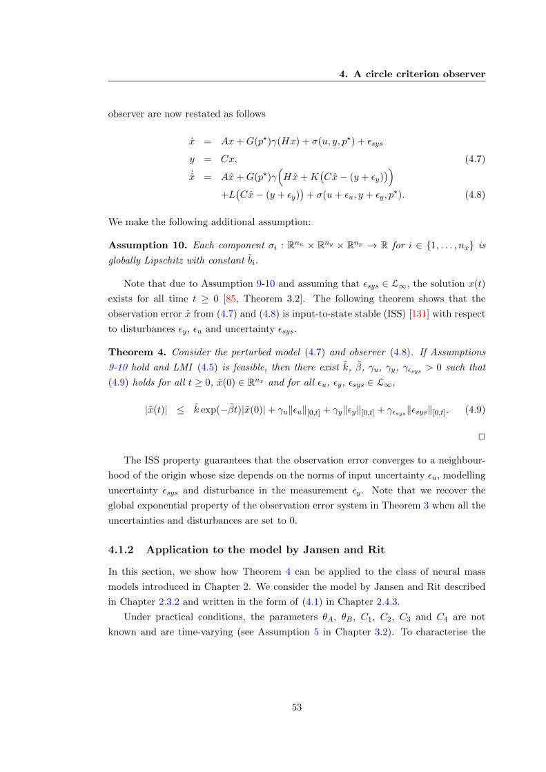
4. A circle criterion observer
observer are now restated as follows
x = Ax+G(p?)γ(Hx) + σ(u, y, p?) + εsys
y = Cx, (4.7)
˙x = Ax+G(p?)γ(Hx+K
(Cx− (y + εy)
))+L(Cx− (y + εy)
)+ σ(u+ εu, y + εy, p
?). (4.8)
We make the following additional assumption:
Assumption 10. Each component σi : Rnu × Rny × Rnp → R for i ∈ {1, . . . , nx} is
globally Lipschitz with constant bi.
Note that due to Assumption 9-10 and assuming that εsys ∈ L∞, the solution x(t)
exists for all time t ≥ 0 [85, Theorem 3.2]. The following theorem shows that the
observation error x from (4.7) and (4.8) is input-to-state stable (ISS) [131] with respect
to disturbances εy, εu and uncertainty εsys.
Theorem 4. Consider the perturbed model (4.7) and observer (4.8). If Assumptions
9-10 hold and LMI (4.5) is feasible, then there exist k, β, γu, γy, γεsys > 0 such that
(4.9) holds for all t ≥ 0, x(0) ∈ Rnx and for all εu, εy, εsys ∈ L∞,
|x(t)| ≤ k exp(−βt)|x(0)|+ γu‖εu‖[0,t] + γy‖εy‖[0,t] + γεsys‖εsys‖[0,t]. (4.9)
2
The ISS property guarantees that the observation error converges to a neighbour-
hood of the origin whose size depends on the norms of input uncertainty εu, modelling
uncertainty εsys and disturbance in the measurement εy. Note that we recover the
global exponential property of the observation error system in Theorem 3 when all the
uncertainties and disturbances are set to 0.
4.1.2 Application to the model by Jansen and Rit
In this section, we show how Theorem 4 can be applied to the class of neural mass
models introduced in Chapter 2. We consider the model by Jansen and Rit described
in Chapter 2.3.2 and written in the form of (4.1) in Chapter 2.4.3.
Under practical conditions, the parameters θA, θB, C1, C2, C3 and C4 are not
known and are time-varying (see Assumption 5 in Chapter 3.2). To characterise the
53

4. A circle criterion observer
uncertainty in the parameters, we introduce εp so that the true parameter of the system
(4.1) is p?+εp, where εp is bounded and unknown. Therefore, the model (4.1) becomes:
x = Ax+G(p? + εp)γ(Hx) + σ(u, y, p? + εp),
y = Cx. (4.10)
Moreover, the EEG measurement y is not noise-free and the input u from afferent
populations is not quantifiable in practice. As performed in Section 4.1.1, we introduce
εy to characterise measurement noise such that the EEG measurement available to the
observer is now y + εy and the input u is allowed to be uncertain by introducing εu
such that the input available to the observer is u+ εu.
We consider the observer in the form of (4.8) as follows:
˙x = Ax+G(p?)γ(Hx+K(p?)
(Cx− (y + εy)
))+σ(u+ εu, y + εy, p
?) + L(p?)(Cx− (y + εy)), (4.11)
where K(p?) and L(p?) are obtained by solving LMI (4.5).
Note that as the LMI (4.5) is dependent on G(p?), verifying that (4.5) is satis-
fied for p? ∈ Θ := [θAmin , θAmax ] × [θBmin , θBmax ] × [C1min , C1max ] × [C2min , C2max ] ×[C3min , C3max ] × [C4min , C4max ] will require infinite number of LMIs to be checked. To
avoid this, we proceed as follows. We note that G(p?) is:
G(p?) = (0, θ1a, 0, θ2b, 0, 0, 0, 0), (4.12)
where θ := (θ1, θ2) = (θAC2, θBC4). Henceforth, we denote G(p?) as G(θ) with slight
abuse of notation. The tuple of parameters (θ1, θ2) takes values in the convex set
Θ := [θ1, θ1]× [θ2, θ2], where θ1 = θAmaxC2max , θ1 = θAminC2min , θ2 = θBmaxC4max and
θ2 = θBminC4min . The vertices of Θ are then:θ?1 = (θ1, θ2)
θ?2 = (θ1, θ2)
θ?3 = (θ1, θ2)
θ?4 = (θ1, θ2).
(4.13)
We now show that if LMI (4.5) is solvable for each θ?i ∈ Θ, i ∈ {1, . . . , 4} with the same
positive definite matrix P = P T , then it is solvable for any p? ∈ Θ. In that way, only
four LMIs need to be verified to ensure the feasibility of (4.5). Due to the convexity of
54

4. A circle criterion observer
Θ, any point θ = (θ1, θ2) ∈ Θ can be written in the form of:
θ =
4∑i=1
λiθ?i (4.14)
where λi ≥ 0, i ∈ {1, . . . , 4} and∑4
i=1 λi = 1. From (4.12), G(θ) is linear in θ, hence:
G(θ) =4∑i=1
λiG(θ?i ). (4.15)
Now, we convert the matrix inequality of Theorem 3 into the following LMI as explained
in [16]:
Mθ(P,R, S,Λ, ν) =[ATP + PA+RC + CTRT + νI PG(p?) +HTΛ + CTST
G(p?)TP + ΛH + SC −2Λdiag(b−11 , . . . , b−1
m )
]≤ 0
(4.16)
where R = PL and S = ΛK. Suppose that there exist positive definite matrix P = P T ,
matrices Ri and Si, positive definite diagonal matrix Λi and strictly positive constant
νi for i ∈ {1, . . . , 4} such that the following holds:
Mθ?i(P,Ri, Si,Λi, νi) ≤ 0, (4.17)
for each vertex θ?i defined in (4.13). Consider θ ∈ Θ, we know that there exist λi such
that (4.14) holds for all λi ≥ 0 and∑4
i=1 λi = 1. Due to the linearity of Mθ(P,R, S,Λ, ν)
in its arguments and (4.15), the following is satisfied:
Mθ(P,R, S,Λ, ν) =4∑i=1
λiMθ?i(P,Ri, Si,Λi, νi), (4.18)
where R =∑4
i=1 λiRi, S =∑4
i=1 λiSi, Λ =∑4
i=1 λiΛi is a positive definite diagonal
matrix and ν =∑4
i=1 λiνi > 0. Consequently, the feasibility of all the LMIs (4.17) for
all i ∈ {1, . . . , 4} with the same P implies that the LMI (4.5) (equivalently (4.16)) is
satisfied for all θ ∈ Θ. Note that the same P that satisfies LMI (4.16) also has to work
for all LMIs (4.17) for i ∈ {1, . . . , 4}, i.e. we have a simultaneous Lyapunov function for
all vertices [85, Section 10.1.3]. We have computationally verified that the LMIs (4.17)
are satisfied for the numerical values provided in [74, Section 2.3]. Therefore, we are
able to state the following result which guarantees the existence of observer matrices
55

4. A circle criterion observer
K(p?) and L(p?) for all p? ∈ Θ such that the state estimation error system x is ISS
with respect to the input and parameter uncertainties εu, εp as well as measurement
noise εy.
Proposition 1. Consider the perturbed model (4.10) and observer (4.11). For any
p? ∈ Θ (where Θ is a compact set), there exist observer matrices L(p?) and K(p?)
that satisfy LMI (4.5) such that the observation error system x satisfies for all t ≥ 0,
x(0) ∈ R8 and for all εu, εy, εp ∈ L∞,
|x(t)| ≤ k exp(−βt)|x(0)|+ γy‖εy‖[0,t] + γu‖εu‖[0,t] + γp‖εp‖[0,t], (4.19)
where k, β, γy, γu, γp ≥ 0. 2
Similar results can be derived for the models by Stam et. al. [138] (described in
Chapter 2.3.3) and Wendling et. al .[155] (described in Chapter 2.3.1) respectively. We
have verified that the conditions of Theorem 4 and Proposition 1 are met.
4.1.3 Simulation results
We show the simulation results for the model (4.10) and observer (4.8). The simulations
are performed under two scenarios: (1) without disturbances and uncertainties, (2)
under the more practical condition with disturbances and uncertainties.
We initialise the model at x(0) = (6, 6, 6, 6, 6, 6, 6, 6) and the observer at x(0) =
(0, 0, 0, 0, 0, 0, 0, 0). The input to the model u as described in [74] is uniformly dis-
tributed between 120 and 320mV. The parameters were chosen to correspond to alpha-
like activity p? = (θA, θB, C1, C2, C3, C4) = (3.25, 22, 135,108, 33.75, 33.75) as identified
in [74]. All other constants used in simulation are as described in [74, Section 3.1].
By solving the LMI (4.5), we obtain the observer matrices L = 104 × (0.0053,
−2.2306, 0.0077, 5.3849, 0.0032,−0.1266,−0.0017, 0.0514) and K = (−0.0586,−0.1422).
Scenario 1: the ideal condition without disturbance and uncertainties
In the ideal scenario, Theorem 3 states that the observer provides estimates that con-
verge to the true states in exponential time. As illustrated in Figure 4.1(a), at t = 0.5s,
the absolute observation error is less than 0.01%.
56

4. A circle criterion observer
Scenario 2: robustness of the observer towards uncertainty in parameters,
input and measurement
We now introduce parameter uncertainty that is 10% of the actual values εp = 0.1 ×(θA, θB, C1, C2, C3, C4) = (0.33, 2.2, 13.5, 10.8, 3.375, 3.375), input uncertainty
εu ∼ N(0, 102) and measurement noise εy ∼ N(0, 0.72), as shown in our perturbed model
(4.10) and observer (4.8). Our simulation results (Figure 4.1(b)) confirm the results
stated in Proposition 1, i.e. the norm of the observation error is small with small L∞
norm of the uncertainties. The absolute observation error relative to the amplitude of
the signal as shown in Figure 4.1(b) remains less than 25% for all states.
0 0.50
0.2
0.4
R.e.x11
0 0.50
0.2
0.4
R.e.x12
0 0.50
0.5
R.e.x21
0 0.50
0.2
0.4
R.e.x22
0 0.50
1
2
R.e.x31
0 0.50
0.5
1
R.e.x32
0 0.50
0.2
0.4
Time, t (s)
R.e.x41
0 0.50
0.2
0.4
Time, t (s)
R.e.x42
(a) Scenario 1: the ideal condition withoutdisturbance and uncertainties.
0 0.50
0.2
0.4
R.e.x11
0 0.50
0.1
0.2
R.e.x12
0 0.50
0.2
0.4R.e.x21
0 0.50
0.2
0.4
R.e.x22
0 0.50
0.5
1
R.e.x31
0 0.50
0.5
1
R.e.x32
0 0.50
0.2
0.4
Time, t (s)
R.e.x41
0 0.50
0.1
0.2
Time, t (s)
R.e.x42
(b) Scenario 2: robustness of the observer to-wards uncertainty in parameters, input andmeasurement
Figure 4.1: Absolute observation error relative to the amplitude of the signal,|xi|
|max(xi)−min(xi)| , for i ∈ {1, . . . , 4}.
4.2 A robust circle criterion observer
In the previous section, we analysed the robustness of the designed observer a posteriori
and showed that it is robust towards disturbances and uncertainty. In this section, we
improve the circle criterion observer designed in Section 4.1 such that it is a priori
57

4. A circle criterion observer
robust towards measurement noise and input uncertainty by providing the user with
the ability to attenuate the effect of noise and uncertainty. To this end, we take into
account measurement noise (Assumption 7) when considering the class of systems
x = Ax+G(p?)γ(Hx) +Bu
y = Cx+Dw, (4.20)
where w ∈ Rnw is the measurement noise. We make the same assumptions about γ as
done previously in Section 4.1.
We consider the following type of observer [17]
˙x=Ax+Gγ(Hx+K(Cx− y)
)+L(Cx− y)+B(u+ d), (4.21)
where x is the state estimate, d ∈ Rnd is the input disturbance and K, L are the
observer matrices to be designed.
As done in [17], denoting the observation error as x := x − x, v := Hx and z :=
Hx + K(Cx − y), the observation error system from (4.20) and (4.21) is ˙x = (A +
LC)x−LDw+Bd+G(γ(z)− γ(v)
). By (4.3), we obtain the observation error system
as
˙x = (A+ LC)x− LDw +Bd+Gδ(t)η, (4.22)
where δ(t) = diag(δ1(t), . . . , δm(t)) and η := z − v.
Given the observation error system (4.22), our task is to find observer matrices K
and L such that a quadratic Lyapunov function V (x) satisfies the following along the
solutions of (4.22)
V (x) ≤ −|x|2 + µw|w|2 + µd|d|2. (4.23)
We can then show that the observation error x satisfies the following property1 for
all t ≥ 0
‖x(t)‖2 ≤ c|x(0)|+√µw‖w(t)‖2 +√µd‖d(t)‖2, (4.24)
where scalars c, µw, µd > 0. The disturbance gains from w and d to x are√µw and
õd respectively.
1We can obtain (4.24) from (4.23) by following the same procedure as in the proof ofTheorem 5.2 in [86].
58

4. A circle criterion observer
4.2.1 Main result
In Theorem 5, we establish that the observation error system (4.22) satisfies property
(4.24) provided that a linear matrix inequality (LMI) is satisfied.
Theorem 5. Consider system (4.20) and observer (4.21). Under Assumption 9, if
there exist a real symmetric and positive definite matrix P , a diagonal and positive
definite matrix M = diag(m1, . . . ,mnm), and scalar constants µw, µd > 0, such that the
following is satisfiedA(P, PL) B(P,M,KTM) −PLD PB
? E(M) −MKD 0
? ? −µwI 0
? ? ? −µdI
≤ 0, (4.25)
where A(P, PL) = P (A+LC)+(A+LC)TP+I, B(P,M,KTM) = PG+(H+KC)TM
and E(M) = −2Mdiag(
1b1, . . . , 1
bnm
), then the observation error system satisfies prop-
erty (4.24). 2
The proof of Theorem 5 is provided in Appendix B.6. Theorem 5 shows that if a K
and L can be found such that the LMI (4.25) is satisfied, then an observer (4.21) can
be designed for system (4.20). Note that condition (4.25) is considered an LMI in P ,
PL, MK, M , µw and µd. As such, (4.25) can be solved using efficient software tools
such as the LMI Lab in MATLAB.
By considering the system (4.20) under the ideal condition where there is no input
uncertainty and measurement error as done in Section 4.1, we obtain the condition
stated in Theorem 3. Current circle criterion results in [17], [45], [158] yield LMIs that
are not feasible for the class of neural models we consider. Therefore, we adapted [45] to
the case where the nonlinearity γ is globally Lipschitz and also monotonically increasing
with inspiration from [17]. This result is a special case of the system considered in
Theorem 5 as stated in Theorem 3 and was reported in [35]. In this section, we further
improve the circle criterion observer obtained in [35] by designing observer matrices
K and L under the circle criterion condition and taking input uncertainty d from
(4.21) and measurement noise w from (4.20) into account. The LMI (4.25) differs from
(13) obtained in [158] in the sense that we consider input uncertainty attenuation and
introduced a multiplier M in components (1, 2), (2, 2) and (2, 3) of (4.25). Without
introducing the multiplier M , the results obtained in [158] do not lead to feasible LMIs.
This simple extension allows circle criterion observers to be designed for the neural
59

4. A circle criterion observer
models we consider, in addition to taking into account the realistic issues faced when
implementing these observers in the context of estimation for neuroscientific studies.
The constants µw and µd in (4.25) may be specified by the user and should the LMI
(4.25) be found to be solvable, we then have the estimation error satisfying property
(4.24) with estimates of the disturbance gainsõw and
õd. In some cases, we may
wish to minimise these constants and various methods are available to solve this multi-
objective optimisation problem (see [42]). A simple approach that we take in the next
section is to minimise the cost Jmax = max{µw, µd} subject to (4.25).
4.2.2 Application to the model by Jansen and Rit
In this section, we show how Theorem 5 can be applied to the model by Jansen and
Rit described in Chapter 2.3.2 and it can be written in the form of (4.20) with D = 1
and all other variables as defined in Chapter 2.4.3. We introduce input disturbance
d ∼ N(0, 0.12) and measurement noise w ∼ N(0, 0.72). The performance of (A) the
circle criterion observer obtained under the conditions of Theorem 3 that does not
consider the attenuation of input uncertainty and measurement noise is compared with
(B) the robust circle criterion observer derived in Theorem 5. We solved LMI (4.5)
to obtain observer matrices K, L for observer (A). For observer (B), we choose to
minimise µw and µd using the cost function Jmax subject to (4.25) to obtain K and
L. The resulting computed disturbance gains areõw = 706 and
õd = 9.48. In the
simulation that follows, we initialise the model at x(0) = (6, 0.5, 6, 0.5, 6, 0.5, 6, 0.5) and
the observers at x(0) = 0. Figure 4.2 shows that the robust circle criterion observer
obtained in Theorem 5 (Observer (B)) outperforms the observer obtained in Theorem
3 (Observer (A)) in the presence of input uncertainty and measurement noise.
60

4. A circle criterion observer
0 0.50
20
40
x11,x11
0 0.5−2000
02000
x12,x12
0 0.5−100102030
x21,x21
0 0.5−2000
02000
x22,x22
0 0.50246
x31,x31
0 0.5−200−100
0100
x32,x32
0 0.501020
Time, t (s)
x41,x41
0 0.5−500
0500
Time, t (s)
x42,x42
Figure 4.2: Estimated states x converge to a neighbourhood of the true states x.Legend: Observer A (grey), Observer B (red) and Model (black).
4.3 Summary
We have designed a robust circle criterion observer that attenuates input uncertainty
and measurement noise. The synthesis of these observers relies on the feasibility of
an LMI (see Theorems 3 and 5). To the best of our knowledge, no other results in
the literature leads to feasible LMIs for the class of neural mass models we consider
in Chapter 2. We extend these results to obtain feasible LMIs for our examples. As
a result, we sacrifice the generality of the circle criterion observer first proposed by
Arcak and Kokotovic in [16], where the globally Lipschitz property of the nonlinearity
γ in (4.1) is removed. The neural mass models contain a nonlinearity that is globally
Lipschitz, i.e. the sigmoid function defined in (2.4) and (2.7). This provides motivation
to impose a restriction on the nonlinearities (Assumption 9) as done in [17] such that
the LMIs are solvable.
61
4. A circle criterion observer
The circle criterion observers are applicable to any system in the class (4.1) provided
the nonlinearity γ is slope-restricted. The extensions of the circle criterion observer in
the literature presented in this chapter were done such that we have a robust nonlinear
observer for the neural mass models. The robustness property of the circle criterion
observers inspired the usage of these observers in a supervisory setup, developed in
Chapter 6, that enables the estimation of parameters and states using state observers
only.
62

Part II: Parameter and state estimation
In the previous part, we designed state observers under the assumption that the
parameters p∗ are known. For neuroscience applications, the assumption that the
parameters are known is too restrictive and only partially useful. For the purposes of
seizure monitoring and control, the parameters are unknown and need to be estimated.
Hence, in this part, we address the problem of parameter and state estimation
using the setup shown in Figure 4.3 via two methods: an adaptive observer and a
supervisory observer. In Chapter 5, we present an adaptive observer for a class of
systems that encompasses a subset of the class of neural mass models described in
Chapter 2. The parameters and states asymptotically converge to their true values
for all initial conditions. In Chapter 6, we present an alternative parameter and state
estimation method for general nonlinear systems using a multiple-model architecture
usually used for control, known in the literature as supervisory control. We adapt this
architecture for estimation and call it a supervisory observer. Under certain conditions,
we obtain practical convergence of parameters and states.
uModel input, Neural mass
model yModel output,
(EEG measurement)
*, px
Adaptive observer/ Supervisory
observer
xState estimate,
pParameter estimate,
Figure 4.3: Parameter and state estimation
63

Chapter 5
An adaptive observer
This chapter presents an adaptive observer for a class of nonlinear systems that
includes a subset of the neural mass models presented in Chapter 2. We observe
that the models by Stam et al and Jansen et al described in Chapters 2.3.3 and 2.3.2
respectively admit the following general structure
x0 = A0x0 + φ0(y)p?
x1 = A1x1 + φ1(x0, u)p?
y = C1x1,
(5.1)
where x0 ∈ Rn0 , x1 ∈ Rn1 are the states, p? ∈ Rnp is a vector of constant and unknown
parameters, y ∈ Rny is the measurement and u ∈ Rnu is the input.
To the best of our knowledge, there is currently no adaptive observer in the literature
that can be used to estimate the parameters and states of system (5.1). Indeed, most
nonlinear adaptive observers apply to systems for which the nonlinearities depend on
known quantities, see [161] for instance. This is not the case for system (5.1) since φ1
depends on x0 which is not measured. Few designs have been proposed for systems
with state-dependent nonlinear terms, see [148] and the references therein. A notable
exception is the work in [46] which focuses on a class of systems that is very similar
to (5.1). While the nonlinearities in (5.1) satisfy some of the conditions stated in [46],
the problem arises in the linear part which is not of the same form as in [46]. As a
consequence, we need to modify the observer and the technical proof in [46]. This study
extends our previous works described in Chapter 3 [33] and Chapter 4 [34; 35] on the
state estimation of this class of neural mass models.
64

5. An adaptive observer
5.1 Writing the models in the form of (5.1)
In this section, we first show how a single cortical column model of neuronal populations
by Jansen and Rit in [74] and described in Chapter 2.3.2 can be written in the form
of (5.1). We also show that n−interconnected single cortical column models can be
written in the form of (5.1). Note that the A matrix of the two models below do
not satisfy the form of the A matrix in the nonlinear system considered in [46]. This
reaffirms the need to design a new adaptive observer as proposed in this chapter. Our
result applies to any system that can be written in the form of (5.1) and is not limited
to the models described below. Nevertheless, the model by Wendling et al described
in Chapter 2.3.1 cannot be written in the required form (5.1). We will discuss possible
extensions of the result described in this chapter to include a more general class of
nonlinear systems.
5.1.1 A single cortical column model
We are interested in estimating the membrane potential contributions of the pyramidal
neurons, the excitatory and inhibitory interneurons respectively (states) and the synap-
tic gains of the excitatory and inhibitory interneurons (parameters). To do so, the model
can be written in state space form (5.1) by taking the states to be1 x0 = (x01, x02) ∈ R2
and x1 = (x11, . . . , x14) ∈ R4, where x01, x11, x13 are membrane potential contributions
of the pyramidal neurons, the excitatory and inhibitory interneurons respectively, and
x02, x12, x14 are their respective derivatives. The measured output (EEG) is y ∈ R,
u ∈ R is the excitatory input from neighbouring columns which is assumed to be
known and p? = (θA, θB) ∈ Θ ⊆ R2 is a vector of unknown parameters where θA and
θB represent the synaptic gains of the excitatory and inhibitory neuronal populations
respectively. The matrices in (5.1) are defined as
C1 =(
1 0 −1 0), A0 = Aa, A1 = diag(Aa, Ab),
where Aa =
(0 1
−a2 −2a
), Ab =
(0 1
−b2 −2b
).
1According to the notation of [74], x0 = (y0, y3) and x1 = (y1, y4, y2, y5).
65

5. An adaptive observer
The parameters a, b ∈ R>0 are assumed to be known. It has to be noted that the
matrices A0 and A1 are Hurwitz. The nonlinear terms in (5.1) are given by
φ0(y) =
(0 0
aS(y) 0
),
φ1(x0, u) =
0 0
ac2S(c1x01) + au 0
0 0
0 bc4S(c3x01)
.
The parameters c1, c2, c3, c4 ∈ R≥0 are assumed to be known parameters and S denotes
the sigmoid function, for v ∈ R: S(v) = 2e01+er(v0−v)
with known constants e0, v0, r ∈ R>0.
For a detailed description about the model and its parameters, see [74] or Appendix
B.12.
5.1.2 Interconnected cortical column models
We now consider a model of n interconnected cortical columns presented in [154]. This
model is obtained by interconnecting n of the single cortical column models described
in Section 5.1.1, in the manner shown in Figure 5.1. Physiologically, the interactions
between cortical columns are the firing rates of each column S(yi). Hence, a physiolog-
ical interpretation of Figure 5.1 would include the sigmoid block S as part of the single
column model.
The study of the interconnected models has the potential of gaining a better under-
standing of the interactions between different regions, whereby each model represents
a part of the cortex [154]. The strength of their interaction is captured by the linear
gains Kji, for i, j ∈ {1, . . . , n} and i 6= j. The propagation dynamics of the interaction
between these regions is described by:
hd(t) = θAadt exp(−adt), ∀t ≥ 0, (5.2)
where θA, ad are positive constants defined in Table 1 of [154].
We assume that the synaptic gains of the populations θAi and θBi are unknown and
the coupling gains Kji for i, j ∈ {1, . . . , n} and i 6= j are known. The interconnected
models can then be written in the form of (5.1) by taking the states in (5.1) to be1 x0 =
(x101, x
102, x
103, x
104, . . . , x
n01, x
n02, x
n03, x
n04) and x1 = (x1
11, x112, x
113, x
114, . . . , x
n11, x
n12, x
n13, x
n14),
1According to the notation of [154] as x0 = (y10 , y13 , y
16 , y
17 , . . . , y
n0 , y
n3 , y
n6 , y
n7 ) and x1 =
(y11 , y14 , y
12 , y
15 , . . . , y
n1 , y
n4 , y
n2 , y
n5 ).
66
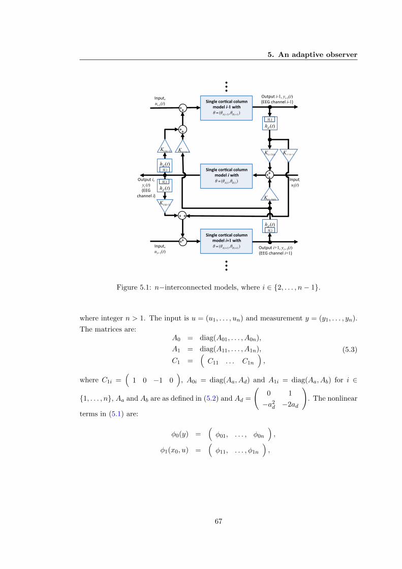
5. An adaptive observer
!"#$%&'ui-1(t)
($%#$%'i-1&'yi-1(t) )**+',-.""/0'i-11'!"#$%&'()*+(,%'()%-.#'
.)/&%'i01'1"23'),( )1()1( !!= iBiA """2'2'
K(i-1)(i)
hd (t)
!"#$%&'()*+(,%'()%-.#'.)/&%'i'1"23'
),( )()( iBiA !!! = !"#$%&'ui(t)
2'2'
!"#$%&'()*+(,%'()%-.#'.)/&%'i41'1"23'
),( )1()1( ++= iBiA !!!!"#$%&'ui+1(t)
($%#$%'i+1&'yi+1(t) )**+',-.""/0'i+11'
K(i+1)(i-1)
($%#$%'i&'yi (t) )**+'
,-.""/0'i1'
2'2'
2'
K(i)(i-1)
2'2'
K(i+1)(i)
hd (t)
2'2'
K(i)(i-1)
hd (t)
hd (t)
K(i-1)(i+1)
S)31'
S)31'
S)31'
S)31'
Figure 5.1: n−interconnected models, where i ∈ {2, . . . , n− 1}.
where integer n > 1. The input is u = (u1, . . . , un) and measurement y = (y1, . . . , yn).
The matrices are:A0 = diag(A01, . . . , A0n),
A1 = diag(A11, . . . , A1n),
C1 =(C11 . . . C1n
),
(5.3)
where C1i =(
1 0 −1 0)
, A0i = diag(Aa, Ad) and A1i = diag(Aa, Ab) for i ∈
{1, . . . , n}, Aa and Ab are as defined in (5.2) and Ad =
(0 1
−a2d −2ad
). The nonlinear
terms in (5.1) are:
φ0(y) =(φ01, . . . , φ0n
),
φ1(x0, u) =(φ11, . . . , φ1n
),
67

5. An adaptive observer
where for i ∈ {1, . . . , n},
φ0i =
0 0
aS(yi) 0
0 0
adS(yi) 0
, φ1i =
0 0
aui + ac2S(c1xi01)
+∑
j∈{1,...,n},j 6=iKjixj03 0
0 0
0 bc4S(c3xi01)
.
5.2 Problem formulation
For ease of notation, we write (5.1) in the following form:
x = Ax+ φ(y, u, x)p?
y = Cx,(5.4)
where x = (x0, x1), A = diag(A0, A1), C = (0, C1) and φ = (φ0, φ1). The nonlinear
terms φ0 : R → Rn0 × Rp and φ1 : Rn0 × Rnu → Rn1 × Rp are globally Lipschitz and
bounded.
Our objective is to synthesise an adaptive observer to simultaneously estimate the
state x and parameter p? of (5.1) from the measured output y. We make the following
crucial assumptions in the design of the adaptive observer:
Assumption 11. The vector of unknown parameters θ is constant and is known to
reside in a compact set Θ.
This assumption is justified under the circumstances where the parameters are slowly-
varying for each type of cortical activity [74]. When a change in activity occurs, an
abrupt variation of p? is presumed which violates Assumption 11 for only a short time
as illustrated in simulations in Chapter 5.4. For the models described in Chapter 5.1,
the plant’s parameters p? were identified to lie in a compact set in Sections 3.1 and 3.2
of [74] respectively.
Assumption 12. The input u is known.
This is a limiting assumption in practice as the input is unknown/unmeasured. A
common assumption is to model the input as random white noise, see [74; 154].
Assumption 13. The measured output y is noise-free.
This assumption is more justified when electroencephalogram (EEG) recorded with
intracranial electrodes as opposed to EEG obtained from electrodes placed on the scalp.
68

5. An adaptive observer
We investigate the robustness of our algorithm to measurement noise in simulations in
Chapter 5.4.
5.3 Main result: an adaptive observer
The adaptive observer synthesised in this chapter draws upon the design by Zhang in
[160] for linear systems and Farza et. al. in [46] for a class of systems that differs from
the class we consider (5.1) in its linear part. Hence, we modified the observer in [46]
and derive a design as presented in the following:
˙x =Ax+ φ(y, u, x)p+ Γ(y − y)
y = Cx˙p = Γ(y − y)
Υ = AΥ + ∆φ(y, u, x) with Υ(0) = 0
P = dP − dPΥTCTCΥP with P (0) = P (0)T > 0,
(5.5)
where Γ = ∆−1ΥΓ, Γ = PΥTCT and ∆ = diag(In0 ,1dIn1) with d > 0 a design param-
eter. The vector x denotes the estimate of x and p the estimate of p?. The variable
Υ ∈ R(n0+n1)×np is initialized to Υ(0) = 0 in order to simplify the technical statements.
Our result also applies when it is not the case. An essential assumption for our design
to work is the condition stated below.
Assumption 14. For any signals u, y, x that belong to L∞, there exist a1, a2 ∈ R>0,
T ∈ R>0 such that the solution to:
Υ = AΥ + ∆φ(y, u, x) with Υ(0) = 0, (5.6)
satisfies for all1 t ≥ 0:
a1Inp ≤∫ t+Tt ΥT(τ)CTCΥ(τ) dτ ≤ a2Inp . (5.7)
2
The condition (5.7) is known as the persistency of excitation of the signal CΥ(t)
and is a well-known condition in identification and adaptive control literature (see [71]).
1A unique solution exists for all time, for all the ordinary differential equations in (5.4) and(5.5). By Theorem 3.3 of [86], P = dP − dPΥTCTCΥP in (5.5) has a unique solution becauseits right hand side is locally Lipschitz and piecewise continuous in t and all its solution are ina compact set (by Lemma 1 of [162], P is bounded). The other ODEs in (5.4) and (5.5) haveunique solutions because the nonlinearity φ is globally Lipschitz.
69

5. An adaptive observer
This is a sufficient condition for the identification of the parameter p? using the adaptive
observer proposed here and it is similar to the condition used in (A4) of [46] and (A3)
in [24]. Inequality (5.7) is hard to verify analytically in general. Nevertheless, we have
observed in simulations that this condition is satisfied for the model we consider under
the simulation conditions stated in Chapter 5.4.
The condition (5.7) is needed to ensure that the solution to P = dP−dPΥTCTCΥP
in (5.5) is symmetric and positive definite for all positive time and with lower and upper
bound which are independent of d, see Lemma 1 in [162]. This is a crucial property
because the matrix P will be used to construct a Lyapunov function in the proof.
We are now ready to state the main result which ensures the asymptotic convergence
of the estimated variables (x, p) to (x, p?). Its proof is given in the Appendix.
Theorem 6. Consider the system (5.4) and the observer (5.5) and suppose Assump-
tions 11-14 are satisfied. Then, there exists d? ≥ 1 such that for all d ≥ d?, the
estimates (x, p) asymptotically converge towards (x, p?) i.e. for any d ≥ d?, there exist
βd ∈ KL such that for any input u and any initial conditions P (0) = P (0)T > 0, x(0)
and p(0), the following holds :
|(x(t), p(t))| ≤ βd(|(x(0), p(0))| , t
)∀t ≥ 0, (5.8)
where x := x− x and p := p? − p. 2
Remark 4. The design parameter d is chosen such that d ≥ d? to obtain (5.8). An
estimate of d?, which we believe is subject to some conservatism is provided in the proof
of Theorem 6 (see (B.28) in the Appendix). Although the expression of d? depends on
|p?|, it is possible to estimate it by taking the maximum over the set Θ, where p? is
known to belong to according to Assumption 11.
5.4 Simulations
We have performed simulations for the single cortical column model described in Section
5.1.1 with the following initial conditions: x(0) = (0.6, 1, 0.6, 1, 0.6, 1), x(0) = 0, p? =
(θA, θB) = (3.25, 22), p(0) = 0, P (0) = I2, Υ(0) = 0. The other parameters take the
value given in [74] and the input is a Gaussian noise of mean 100 and variance 302.
Figures 5.2(a)-5.2(b) respectively show the state and parameter estimation error when
the design parameter d is equal to 2 and 10. They confirm the convergence properties
of the algorithm and show that larger d speeds up the rate of convergence.
70

5. An adaptive observer
0 1 20
0.5
1|x
01
−x01|
0 1 20
20
40
|x02
−x02|
0 1 20
10
20
|x11
−x11|
0 1 20
500
1000
|x12
−x12|
0 1 20
10
20
Time, t (s)
|x13
−x13|
0 1 20
500
1000
Time, t (s)
|x14
−x14|
(a) State estimation error for d = 10.
0 5 10 152
0
2
4
0 5 10 1510
0
10
20
30
Time, t (s)
θA
θA with d = 2
θA with d = 10
θB
θB with d = 2
θB with d = 10
(b) Parameter estimates for d = 2 and 10.
As previously mentioned, Assumptions 11 and 13 (i.e parameters are constant and
noise-free measurement) are limiting assumptions in practice. In Figure 5.2(c), we sim-
ulate a change in parameters which might correspond to a change in cortical activity.
We see that the estimated parameters still converge to the true values after the tran-
sition has occurred. We also consider the scenario where the measured output (EEG)
is noisy by introducing a random noise that is drawn from a Gaussian distribution of
mean 0 and variance 0.42, which is approximately 20% of y at steady state. Figure
5.2(d) shows that despite the presence of measurement noise, the adaptive observer
still provides estimates that are close to the true values. In fact, the neighbourhood
in which the parameter error converges to is smaller with small d. This illustrates the
tradeoff between fast convergence rate and robustness towards measurement noise.
5.5 Summary
We have presented an algorithm to provide simultaneous estimates of the states and
parameters of a class neural mass models using the electroencephalogram (EEG) as the
measured output. This adaptive observer is based on the work in [46], where the class
of systems considered are different in the linear part. Consequently, modifications were
made in the adaptive observer and we provided a technical proof for the asymptotic
71

5. An adaptive observer
0 5 10 15 203
4
5θ
A
0 5 10 15 2015
20
25
θB
0 5 10 15 200
2
4
|θA
−θ
A|
0 5 10 15 200
20
40
Time,t ( s)
|θB
−θ
B|
(c) Parameter estimation error with varyingparameters for d = 10.
0 5 10 152
0
2
4
0 5 10 1510
0
10
20
30
Time, t (s)
θB
θB with d = 2
θB with d = 10
θA
θA with d = 2
θA with d = 10
(d) Parameter estimates with noisy measure-ment for d = 2 and 10.
convergence of parameters and states. Simulations are provided for a single cortical
column model by [74] which confirm our results. As with the state observer designed in
Chapter 4, the adaptive observer synthesised in this chapter is applicable to any system
in the class considered (5.1) and not limited to the neural mass models in Chapter 2.
In reality, the parameters of the system varies as the brain transitions from one
event to another, e.g. non-seizure to seizure activity. The assumption we made in
our design (Assumption 11) is restrictive in that the parameters are assumed to be
constant. However, we expect our results to hold provided that the parameters are
slowly-varying, see Chapter 9.6 in [86] for a discussion on slowly varying systems.
We also employ the constant parameter assumption in the next chapter, where we
provide an alternative estimation method for states and parameters using the supervi-
sory architecture.
72

Chapter 6
Supervisory observer
In this chapter, we present a parameter and state estimation algorithm for general
nonlinear systems, which we call a supervisory observer. We adopt an architecture
known as the supervisory framework used in [95, Chapter 6] that is used for control (see
[64; 66; 110; 152] for linear systems and [21] for nonlinear systems). In these works, the
objective is to steer the plant’s state to the origin and no guarantee is provided on the
parameter and state estimates. Since our objective is to estimate and not to control,
we adopt the supervisory setup without the multi-controller and adapt the available
results, so that it is applicable for estimation.
The plant’s parameters are assumed to be constant and they belong to a known,
compact parameter set. We sample the parameter set to form a finite set of nominal pa-
rameter values. The distribution of these sampled parameters can be done based upon
prior knowledge of the plant’s unknown parameters. An observer with a robustness
property is designed for each of the parameter values, which forms a bank of observers
known as the multi-observer. The supervisory unit chooses an observer from the multi-
observer based on a criterion using a logical decision rule that generates a piecewise
constant signal that is the index of the chosen observer at every instant of time. We
use the scale-independent hysteresis switching logic introduced in [64]. The selected
observer at each time provides us with a state estimate and its corresponding parameter
estimate. In this chapter, we assume that the solution of the plant’s state is uniformly
bounded and all the output estimation errors of the multi-observer satisfy a persistency
of excitation (PE) property. The parameter and state estimation error are guaranteed
to converge to the origin with some margin of error, provided that the sampling of the
parameter set is sufficiently large such that the distance from the plant’s parameter to
the sampled parameter set is small enough.
73

6. Supervisory observer
We believe that the advantages of supervisory control discussed in [65] translate
well to the problem of state and parameter estimation. Firstly, it is not necessary to
construct an adaptive observer, which is a challenging problem for nonlinear systems. In
fact, very few provable designs exist, especially for nonlinearly parameterised systems
(see [46] and the references there-in). Secondly, the supervisory framework has the
advantage of modularity. Each of the components: the switching logic, the monitoring
signals and the multi-observer can be designed independently to satisfy the respective
properties required to meet our objective. This allows for the usage of readily available
state observers for the additional purpose of parameter estimation. In Section 6.4, we
design Luenberger observers for linear systems and a robust form of circle criterion
observers [34] (Chapter 4.2) for a class of nonlinear systems. Finally, in Section 6.5, we
show that this setup can be applied to the neural mass models in Chapter 2.
6.1 Problem formulation
We consider the following class of nonlinear systems
x = f(x, p?, u)
y = h(x, p?), (6.1)
where the state vector is x ∈ Rnx , the output is y ∈ Rny , the input is u ∈ Rnu and
the unknown parameter vector p? ∈ Θ ⊂ Rnp is constant, where Θ is a known compact
set. For any initial condition x(0) and input u ∈ M∆u , where ∆u > 0, system (6.1)
admits a unique solution x(·, x(0), u[0,t], p?) that is defined for all positive time. The
short hand notation x(·) will often be used instead when there is no ambiguity from
the context. The following additional assumptions are made on the plant.
Assumption 15. The function h : Rnx ×Rnp → Rny is continuously differentiable. 2
Assumption 16. The solutions of system (6.1) are uniformly bounded, i.e for all ∆x,
∆u ≥ 0, there exists a constant Kx = Kx(∆x,∆u) > 0 such that for all (x(0), u) ∈B∆x ×M∆u
|x(t)| ≤ Kx, ∀t ≥ 0. (6.2)
2
At this stage, it is important to note that the neural mass models discussed in
Chapter 2 satisfy this assumption. We will show how to apply the general results to
the model by Jansen and Rit later in Section 6.5.
74

6. Supervisory observer
Remark 5. Contrary to the problem of supervisory control in [151] and [152], we do
not require the system (6.1) to be stabilisable. Since our purpose is to estimate, we only
require the solutions of system (6.1) to be uniformly bounded.
The main objective of this paper is to estimate the parameters p? and the states x
of system (6.1) when only the input u and the output y of system (6.1) is measured,
using the supervisory observer which is described in the next section.
6.2 Supervisory observer
Based on the supervisory framework used for control in [152], the proposed methodology
consists of two basic units: a bank of observers (multi-observer) which generates state
estimates and the supervisor (monitoring signals and switching logic) which chooses
one observer as shown in Figure 6.1. The estimated parameters and states are derived
from the choice the supervisor makes.
Plant *),(
)*,,(
pxhy
upxfx
),ˆ(ˆ
),,,ˆ(ˆˆ
111
111
pxhy
yupxfx
),ˆ(ˆ
),,,ˆ(ˆˆ
NNN
NNN
pxhy
yupxfx
Swit
chin
g Lo
gic
Esti
mat
or
Multi-observer
)(ˆ1ty
)(ˆ tyN
Supervisor
)(t)(ˆ tx
)(ˆ tp
)(tu )(ty
Figure 6.1: Supervisory observer.
6.2.1 Sampling of the parameter set Θ
We choose N distinct parameter values from the known, compact parameter set Θ.
Thus, they form a sampled parameter set denoted Θo := {p1, . . . , pN} ⊂ Θ. We denote
the induced parameter error set as Θ := {pi − p? : p? ∈ Θ, pi ∈ Θo, i ∈ {1, . . . , N}}.The distribution of the sampled parameters can be logarithmic as shown in Figure
6.2, where more pi’s are chosen in regions where the plant’s parameter p? is expected to
75
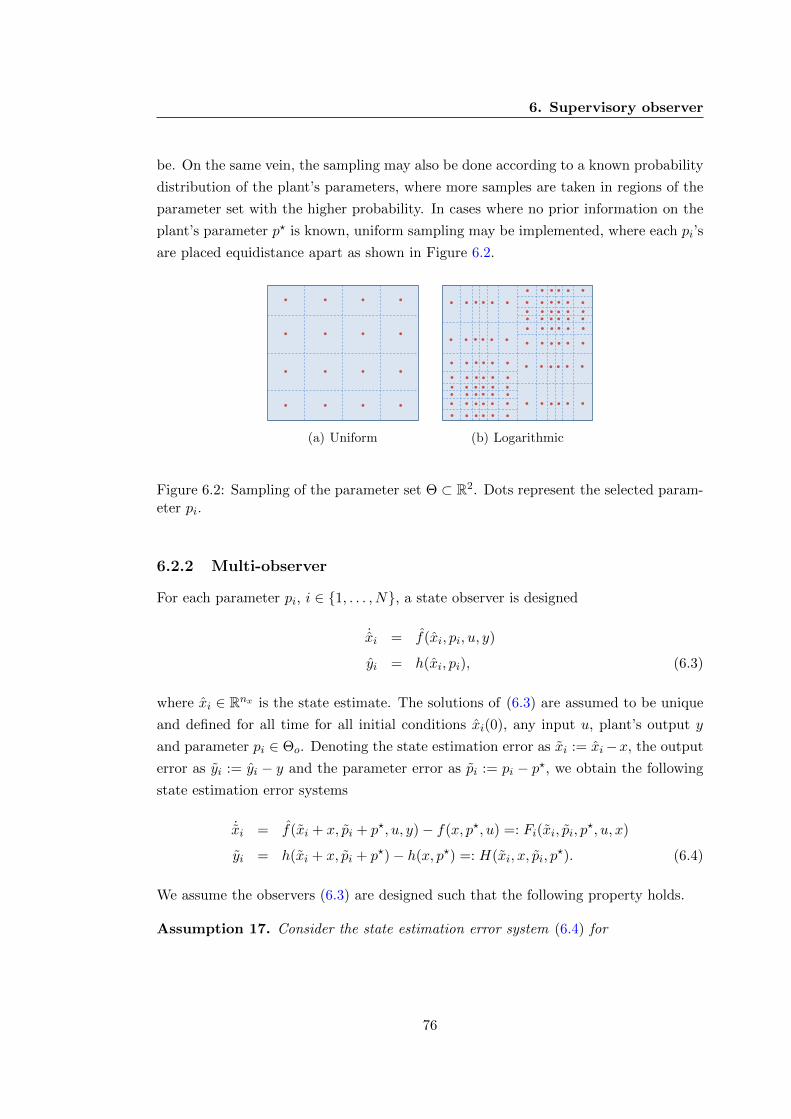
6. Supervisory observer
be. On the same vein, the sampling may also be done according to a known probability
distribution of the plant’s parameters, where more samples are taken in regions of the
parameter set with the higher probability. In cases where no prior information on the
plant’s parameter p? is known, uniform sampling may be implemented, where each pi’s
are placed equidistance apart as shown in Figure 6.2.
(a) Uniform (b) Logarithmic
Figure 6.2: Sampling of the parameter set Θ ⊂ R2. Dots represent the selected param-eter pi.
6.2.2 Multi-observer
For each parameter pi, i ∈ {1, . . . , N}, a state observer is designed
˙xi = f(xi, pi, u, y)
yi = h(xi, pi), (6.3)
where xi ∈ Rnx is the state estimate. The solutions of (6.3) are assumed to be unique
and defined for all time for all initial conditions xi(0), any input u, plant’s output y
and parameter pi ∈ Θo. Denoting the state estimation error as xi := xi−x, the output
error as yi := yi − y and the parameter error as pi := pi − p?, we obtain the following
state estimation error systems
˙xi = f(xi + x, pi + p?, u, y)− f(x, p?, u) =: Fi(xi, pi, p?, u, x)
yi = h(xi + x, pi + p?)− h(x, p?) =: H(xi, x, pi, p?). (6.4)
We assume the observers (6.3) are designed such that the following property holds.
Assumption 17. Consider the state estimation error system (6.4) for
76

6. Supervisory observer
i ∈ {1, . . . , N}. There exists a continuously differentiable function Vi : Rnx → R≥0,
a continuous positive function γ : Θ × Rnx × Rnu → R≥0 where γ(0, z, z) = 0 for all
z ∈ Rnx, z ∈ Rnu, and constants a1, a2, λ0 > 0, µν ≥ 1 such that the following holds
for all pi ∈ Θ, for all u ∈ Rnu, xi ∈ Rnx, x ∈ Rnx
a1|xi|2 ≤ Vi(xi) ≤ a2|xi|2, (6.5)
∂Vi∂xi
Fi(xi, pi, p?, u, x) ≤ −λ0Vi(xi) + γ(pi, x, u). (6.6)
2
Assumption 17 implies that the origin of the state estimation error system (6.4) is
globally exponentially stable when pi = p?, i.e. when we know the value of the plant’s
parameters p?. When this is not the case, condition (6.6) needs to be satisfied, which is
a robustness property of system (6.4) with respect to pi. It is noted that Assumption
17 is satisfied when system (6.4) is input-to-state exponentially stable [58, Equation
(5)] with respect to pi. In Section 6.4, we will show that Luenberger observers and
circle criterion observers satisfy Assumption 17.
Following the terminology used in [152], we call the bank of observers in (6.3) a
multi-observer.
Remark 6. If the function γ in (6.6) is dependant only on pi and u, Assumption
16 can be relaxed in the sense that the solutions of (6.1) do not have to be uniformly
bounded. In this case, for all u ∈M∆u, the system (6.4) is locally input-to-state stable
(ISS) [85, Theorem 5.2] with respect to pi.
Remark 7. The Lyapunov-based conditions (6.5)-(6.6) stated in Assumption 17 differ
from the conditions stated in [152, Equations (10a) and (10b)] and [151, Theorem 4.3
(iii)] because our objective is the estimation of the parameters and states of (6.1),
whereas the available results in the literature consider the problem of stabilisation of an
equilibrium point without parameter estimation. Moreover, in the literature, the state
of the stabilised plant converges to zero, whereas in our case, the state of the plant does
not necessarily converge to zero.
77

6. Supervisory observer
6.2.3 Monitoring signal
As used in [152, Equation 6], the monitoring signal associated with each observer is the
exponentially weighted L2 norm [71] of the output error yi defined as
µi(t) =
∫ t
0exp(−λ(t− s))|yi(s)|2ds+ cµ, ∀t ≥ 0, (6.7)
where constants λ and cµ > 0 are design parameters. The signal µi can be implemented
with cµ added to the output of a linear filter
πi = −λπi + |yi|2, (6.8)
with πi(0) = 0. We assume that the output error of each of the observers yi satisfies
the following property.
Assumption 18. Consider the state error system (6.4) for all i ∈ {1, . . . , N}. For
all ∆x, ∆x, ∆u > 0, there exist a constant Tf = Tf (∆x,∆x,∆u) > 0 and a class K
function αy(∆x,∆x,∆u) such that for all xi(0) ∈ B∆x, x(0) ∈ B∆x, for some u ∈M∆u,
and for all pi ∈ Θ, the corresponding solution to (6.4) satisfies∫ t
t−Tf|yi(τ)|2dτ ≥ αy(|pi|), ∀t ≥ Tf . (6.9)
2
The inequality (6.9) is known as a persistency of excitation (PE) condition that
appears in identification and adaptive literature [71]. It differs from the classical PE
definition1 in that we consider here a family of systems parameterised with pi, where
the lower bound (excitation level) in (6.9) depends on pi. In particular, if pi = 0, we do
not necessarily have PE in the classical sense. In addition, the excitation level grows
with the norm of the parameter error pi. Hence, the integral term in (6.9) provides
some quantitative information about the parameter estimation error. Assumption 18
holds when the output errors yi, for i ∈ {1, . . . , N} satisfy the classical PE condition
(6.10) according to the proposition below.
1A vector signal φ : R≥0 → Rn is said to be persistently exciting (PE) with excitation levelα > 0 if there exists a constant T > 0 such that for all t ≥ T∫ t
t−Tφ(s)φ(s)T ds ≥ αI. (6.10)
78

6. Supervisory observer
Proposition 2. Consider the state error system (6.4) for i ∈ {1, . . . , N}. Suppose that
the following holds.
1. Assumption 15 is satisfied.
2. The function f : Rn × Rnp × Rnu → Rn is continuously differentiable.
3. For all ∆x, ∆x, ∆u > 0 and for all pi 6= 0 with pi ∈ Θ, there exist constants Tf =
Tf (∆x,∆x,∆u, pi), αi = αi(∆x,∆x,∆u, pi) > 0 such that for all xi(0) ∈ B∆x,
x(0) ∈ B∆x and for some u ∈ M∆u, the corresponding solution to (6.4) satisfies
the following ∫ tt−Tf |yi(τ)|2dτ ≥ αi, ∀t ≥ Tf . (6.11)
Then (6.9) holds. 2
Proposition 2 indicates that tools to verify the classical PE condition (6.11) (see
[112, Chapter 6] for linear systems and [118] for nonlinear systems) can be applied to
ensure that Assumption 18 is satisfied.
6.2.4 Switching logic
The switching logic σ : [0,∞) → {1, . . . , N} produces a piecewise constant signal
which chooses an observer from the bank of N observers at every instant of time. We
implement the scale-independent hysteresis switching logic [64]
σ(t) :=
arg mini∈{1,...,N}
µi(t), ∃j ∈ {1, . . . , N} such that (1 + h)µj(t) ≤ µσ(t−s )(t)
σ(t−s ), otherwise,
(6.12)
where ts denotes the latest switching time of σ before t. On the occasion where
arg minµi is non-unique, the switching logic σ(t) selects the smallest index i ∈ {1, . . . , N}which satisfies arg minµi. The hysteresis constant h > 0 is a design parameter.
The switching signal σ implemented with the monitoring signals defined in (6.7)
has an average dwell-time (see [95, Section 3.2.2]), i.e. there exist τa, N0 > 0 such
that the number of discontinuities (number of switchings) on an arbitrary time interval
[t0, t) denoted by Nσ(t, t0) satisfies the following
Nσ(t, t0) ≤ N0 +t− t0τa
. (6.13)
79

6. Supervisory observer
This means that there is a finite number of switches in every finite interval, thereby
no Zeno behaviour can occur. The following lemma is shown along the same lines as
[63; 151].
Lemma 1. Consider the plant (6.1), the multi-observer (6.3), the monitoring signal
(6.7) and the switching logic (6.12) under Assumptions 15-18. The number of switchings
of the switching logic σ satisfies (6.13) with
τa := ln(1+h)λN , N0 ≥ 1, (6.14)
where h > 0 is the hysteresis constant from (6.12), λ > 0 is from the monitoring signal
(6.7) and N ≥ 1 is the number of observers in the multi-observer (6.3). 2
6.2.5 Parameter and state estimates
Based on the signal generated by the switching logic σ from (6.12), the estimated
parameters p : [0,∞)→ {p1, . . . , pN} and estimated states x : [0,∞)→ Rn are
p(t) := pσ(t), (6.15)
x(t) := xσ(t)(t), ∀t ≥ 0. (6.16)
The state estimate x is picked from the solutions of a family of observer systems (6.3),
for i ∈ {1, . . . , N}. The chosen state estimate x(t) = xσ(t)(t) as defined in (6.16)
is discontinuous in general, which is caused by the switching between different state
estimates that are in general different at the switching instant ts.
Remark 8. Choosing a solution from a family of systems˙x1 = f(x1, p1, u, y)...
...˙xN = f(xN , pN , u, y),
(6.17)
in the way the estimated state xσ(t) is chosen differs from a switched system with state
jumps, in that we switch among a family of observer systems (6.3) whose solutions do
not get affected by the switching. To be precise, let xi
(t; xi(0)
), for i ∈ {1, . . . , N}
denote the solution of the observer system (6.3) for any xi(0) ∈ B∆x and u ∈ M∆u,
where we have omitted the dependance on u, y and pi. Consider the switching logic
σ with a switching sequence {t1, t2}, where t2 > t1 > 0 and σ(0) = 1, σ(t1) = 2 and
80

6. Supervisory observer
σ(t2) = 1. Our estimated state xσ(t)(t) for all t ≥ 0 is
xσ(t)(t) =
x1
(t; x1(0)
), t ∈ [0, t1)
x2
(t; x2(0)
), t ∈ [t1, t2)
x1
(t; x1(0)
), t ∈ [t2,∞).
(6.18)
This is different from a switched system with state jumps where its solution for all t ≥ 0
is
xσ(t)(t) =
x1
(t; x1(0)
), t ∈ [0, t1)
x2
(t;ϕ(x1(t1)
)), t ∈ [t1, t2)
x1
(t;ϕ(x2(t2)
)), t ∈ [t2,∞),
(6.19)
where ϕ is some jump map.
This distinction is crucial because provided that σ is a piecewise continuous signal,
xσ(t) in (6.18) retains the behaviour of the individual systems (6.3), whereas the solu-
tions of a switched system with state jumps in (6.19) may exhibit a different behaviour
as discussed in Part II of [95]. 2
6.3 Main result
Before stating our main result, we first provide some intuition behind our result. Guide-
lines for the user are then provided to assist in implementing the supervisory observer.
Recall that N distinct parameters pi ∈ Θo for i ∈ {1, . . . , N} are chosen from the
known parameter set Θ and they form the sampled parameter set Θo ⊂ Θ. Let the
point-to-set distance of the plant’s parameter p? to the set of sampled parameters Θo
be
d(p?,Θo) := minpi∈Θo for i∈{1,...,N}
|p? − pi|. (6.20)
We are interested in the scenario where the selected parameters pi’s are distributed in
Θ in a manner that d(p?,Θo) decreases as we increase the number of observers N . Most
notably, as N →∞, d(p?,Θo)→ 0, which forms the main intuition behind Theorem 7
whose proof can be found in Appendix B.10.
Theorem 7. Consider the plant (6.1), the multi-observer (6.3), the monitoring signals
(6.7), the switching logic (6.12), the parameter estimate (6.15) and the state estimate
(6.16). Suppose Assumptions 15-18 hold. For any ∆x, ∆x, ∆u > 0, for all νx, νp > 0,
for all λ, cµ > 0 (as in (6.7)), there exist constants Kx, δ? and h? > 0, such that for
81

6. Supervisory observer
all h ∈ (0, h?], for any Θo with d(p?,Θo) ≤ δ?, there exists a constant T > 0, such that
for all (x(0), xσ(0)(0)) ∈ B∆x × B∆x and for any u ∈ M∆u that satisfies Assumption
18, the following holds
|pσ(t)| ≤ νp, ∀t ≥ T, lim supt→∞ |xσ(t)(t)| ≤ νx, |xσ(t)(t)| ≤ Kx, ∀t ≥ 0.
(6.21)
where pσ(t) := p(t)− p? is the parameter estimation error and xσ(t) := x(t)−x(t) is the
state estimation error. 2
Theorem 7 shows that the parameter and state estimates converge to the true
values with desired accuracy νp and νx respectively, provided that the parameter set Θ
is sampled sufficiently, i.e. the number of observers N is sufficiently large. Moreover,
the state estimation error xσ is guaranteed to be bounded.
We provide some guidelines for the user to implement the algorithm below.
1. The system (6.1) is first verified to satisfy Assumptions 15-16.
2. Selection of parameter values pi: a finite number of parameter values are selected
from the parameter set Θ. Our result hinges upon taking a sufficiently large
sampling of the parameter set in the way that d(p?,Θo) becomes small enough
such that the conclusions of Theorem 7 hold (d(p?,Θo) ≤ d? in Theorem 7). This
may require high computing resources in practice, however the sampling of the
parameter set can be done in efficient ways as discussed earlier in Section 6.2.1.
3. Design of the multi-observer : For each of the sampled parameter values, we
design a state observer (6.3) such that Assumption 17 holds. The synthesis of a
nonlinear state observer is a difficult problem in general. Nevertheless, various
designs are available in the literature for specific classes of systems [23]. Examples
are provided in Section 6.4. Typically, an observer is first designed under the
assumption that the plant’s parameter is known such that the equilibrium of the
state estimation error system is globally exponentially stable. We then either
verify or design each observer such that it satisfies the robustness property (6.6).
4. Satisfaction of the PE condition (6.9) : Assumption 18 may be satisfied with the
aid of Proposition 2. The reader is referred to [112, Chapter 6] and [118] for prop-
erties of PE signals of linear and nonlinear systems respectively to obtain a priori
checkable conditions. Otherwise, Assumption 18 may be checked in simulation
a posteriori since we have access to yi online as illustrated by an example from
neuroscience in Section 6.5.
82

6. Supervisory observer
5. Choice of design parameters h, λ and cµ : The parameters λ and cµ relates di-
rectly to the properties of the switching signal σ. In Lemma 1, it is shown that
the average dwell time of the switching logic σ is τa := ln(1+h)λN . Hence, increasing
λ and choosing a small enough hysteresis constant h (from (6.12)) speeds up the
convergence rate of the parameters.
Consequently, the estimated parameter converges to a ball of a given margin νp centered
at the true parameter p? in finite time and the state estimation error also converges
to a ball of a given margin νx as t → ∞. Additionally, the state estimation error is
bounded.
6.4 Applications
In this section, we investigate two case studies: (i) linear systems, for which Luenberger
observers are designed and (ii) a class of nonlinear systems, for which robust circle
criterion observers (first introduced in [17] and a robust version introduced in [34]) are
synthesised.
6.4.1 Linear systems
We consider a linear plant
x = A(p?)x+B(p?)u
y = C(p?)x, (6.22)
where x ∈ Rnx , u ∈ Rnu , p? ∈ Θ ⊂ Rnp and A(p) is assumed to be Hurwitz, for all
p ∈ Θ. We notice that Assumption 15-16 hold. Note that, although system (6.22) is
linear, it is nonlinearly parameterised. We also assume the following.
Assumption 19. The matrices A(p), B(p) are continuous in p ∈ Θ.
Each observer in the multi-observer is designed as follows for i ∈ {1, . . . , N}
˙xi = A(pi)xi +B(pi)u+ Li(pi)(C(pi)xi − C(p?)x)
yi = C(pi)xi, (6.23)
where Li(pi) is such that A(pi) + Li(pi)C(pi) is Hurwitz (this is always possible since
A(pi) is Hurwitz, for all pi ∈ Θo, where i ∈ {1, . . . , N}). Denoting the state estimation
83

6. Supervisory observer
error as xi := xi − x and the parameter error as pi := pi − p? as in Section 6.2, we
obtain the following state estimation error system
˙xi =(A(pi) + Li(pi)C(pi)
)xi −
(A(p?) + Li(pi)C(p?)
)x+
(B(pi)−B(p?)
)u
=(A(pi) + Li(pi)C(pi)
)xi +
(A(pi, p
?) + Li(pi)C(pi, p?))x
+B(pi, p?)u, (6.24)
where we denote A(pi, p?) := A(pi)−A(p?), B(pi, p
?) := B(pi)−B(p?) and C(pi, p?) :=
C(pi)− C(p?). Proposition 3 shows that Assumption 17 is satisfied.
Proposition 3. Consider the linear system (6.22), the multi-observer (6.23) and sup-
pose Assumption 19 is satisfied. If there exist Pi = P Ti > 0 and scalar constants νi,
µi > 0 such that the following holds[Pi (A(pi) + Li(pi)C(pi)) + (A(pi) + Li(pi)C(pi))
T Pi + νiI Pi
Pi −µiI
]≤ 0. (6.25)
Then Assumption 17 is satisfied. 2
As explained earlier, if the classical PE condition (6.11) is guaranteed, Assumption
18 is satisfied according to Proposition 2. There exist results in the literature (see
Chapter 6 in [112]) which provide sufficient conditions to verify (6.11) for linear systems.
They can be used, for instance, to design an input to the system (6.22) such that the
inequality (6.11) is satisfied. Lastly, since all the conditions of Theorem 7 are satisfied,
we derive the following result.
Proposition 4. Consider the linear system (6.22), the multi-observer (6.23) for i ∈{1, . . . , N}, the monitoring signals (6.7), the switching logic (6.12). Suppose that As-
sumptions 18 and 19 are satisfied, then the conclusions of Theorem 7 hold. 2
Proposition 4 extends the results in [89] from single-input single-output (SISO) to
multi-input multi-output (MIMO) systems.
6.4.2 A class of nonlinear systems
We consider the following class of nonlinear systems first studied in [16] for the design
of circle criterion observers
x = A(p?)x+G(p?)γ(Hx) +B(p?)σ(u, y)
y = C(p?)x, (6.26)
84

6. Supervisory observer
where γ : Rnp → Rnγ and σ : Rnu ×Rny → Rnσ . We assume that Assumption 16 holds
and also make the following assumptions.
Assumption 20. The matrices A(p), G(p) and B(p) are continuous in p ∈ Θ.
Assumption 21. For any k ∈ {1, . . . , nγ}, there exist constants aγk , bγk > 0 such that
the following holds
−∞ < aγk ≤∂γk(vk)
∂vk≤ bγk <∞, ∀vk ∈ R, (6.27)
where γ = (γ1, . . . , γnγ ). 2
By Assumption 21, γ includes nonlinearities that are globally Lipschitz, with bγk =
−aγk . This assumption was used in [158] and is a special case of the assumption in
[17, Equation (1)] and [34, Assumption 1] for differentiable nonlinearities γ. Moreover,
since system (6.26) is assumed to be bounded, there is no loss in generality in assuming
that γ is globally Lipschitz (see for example Section 2 in [46]).
For each pi ∈ Θo, i ∈ {1, . . . , N}, the following observer [17; 34; 158] is designed
˙xi = A(pi)xi +G(pi)γ(Hxi +Ki(Cxi − y)) +B(pi)σ(u, y) + Li(C(pi)xi − y)
yi = C(pi)xi, (6.28)
where Ki and Li are observer matrices designed using the ideas in [34], i.e. such that
a quadratic function Vi : Rnx → R≥0 satisfies the conditions stated in Assumption 17.
Proposition 5. Consider system (6.26) and multi-observer (6.28), for all
(x(0), xi(0)) ∈ B∆x × Rnx and u ∈ M∆u. Under Assumptions 16, 20 and 21, if there
exist matrices Pi = P Ti > 0, Mi = diag(mi1, . . . ,minp) > 0 and scalar constants νi,
µi > 0 such that the following holds A(Pi, Li, νi) B(Pi,Mi,KTi Mi) Pi
? E(Mi) 0
? ? −µiI
≤ 0, (6.29)
where A(Pi, Li, νi) = Pi(A+ Li(pi)C(pi)
)+(A+ Li(pi)C(pi)
)TPi + νiI,
B(Pi,Mi,KTi Mi) = PiG(pi) +
(H +Ki(pi)C(pi)
)TMi and
E(Mi) = −2Midiag(
1bγ1, . . . , 1
bγnp
), then Assumption 17 is satisfied. 2
We assume that the PE condition stated in Assumption 18 is satisfied. PE prop-
erties for nonlinear systems are studied in [118] and may be used in conjunction with
85

6. Supervisory observer
Proposition 2 to obtain checkable PE conditions for some classes of systems. Finally,
we obtain the following result since all the conditions of Theorem 7 hold.
Proposition 6. Consider the nonlinear system (6.26), the multi-observer (6.23), the
monitoring signals (6.7), the switching logic (6.12) and suppose the following hold.
1. Assumptions 16, 18, 20 and 21 hold.
2. Condition (6.29) is feasible.
Then the conclusions of Theorem 7 hold. 2
Proposition 6 extends the results of [45, Theorem 3], [158] and [46], where adaptive
observers are designed, in the sense that we consider a more general class of nonlinearly
parameterised nonlinear systems.
6.5 Illustrative example: A neural mass model by Jansen
and Rit
In this section, we apply the results of Section 6.4.2 to estimate the parameters and the
states of the neural mass model in [74] and described in Chapter 2.3.2. It describes the
dynamics of a single column model by capturing the interactions between the pyramidal
neurons, the excitatory and the inhibitory interneurons in a localised region of the
cortex. The model has been shown to realistically reproduce various patterns, such as
alpha rhythms, seen in the electroencephalogram, also known as EEG (the measured
output). Moreover, the model may be used to capture more complex phenomena as
shown in [155]. The objective in this section is to estimate the mean membrane potential
of neural populations (states x) and the synaptic gains of each of the populations
(parameters p?).
The model can be written in the form (6.26) as shown in Chapter 2.4.3. It also has
uniformly bounded solutions for all initial conditions x(0) and bounded input u ∈M∆u ,
because the matrix A is Hurwitz, the nonlinearity S in γ and σ is bounded. Therefore,
the model satisfies Assumption 16. Furthermore, by the definition of the matrices A,
G, B and the nonlinearity S, Assumptions 20 and 21 are satisfied.
We sample the parameter space non-uniformly by sampling p2 more densely in the
range of 20− 30 (p?2 = 25) and p1 is distributed uniformly. The observers are designed
as proposed in Section 6.4.2. Figure 6.3(d) shows that the classical PE condition (6.11)
seems to be satisfied for when N = 10, 100 and 130. Hence, by Proposition 2, Assump-
tion 18 may be satisfied. Therefore, the conclusions of Theorem 7 hold according to
86

6. Supervisory observer
Proposition 6. We implement the supervisory setup with hysteresis constant h = 0.5,
the design parameters from the monitoring signal (6.7) are λ = 0.005 and cµ = 2. Ta-
ble 6.5 summarises the results for increasing N in such a way that d(p?,Θo) decreases.
Figure 6.3 compares the performance of the algorithm for N = 10, 100 and 130.
N 10 50 100 120 130
d(p?,Θo) 2.2361 1.1180 1.0244 1.0164 1.0035lim supt→∞
|p(t)− p?| 5.385 5.385 5.204 5.233 1.537
lim supt→∞
|x(t)−x(t)||maxt x(t)−mint x(t)| 0.033 0.033 0.031 0.031 0.0898
Table 6.1: Numerical results for increasing N values such that d(p?,Θo) decreases.
0 0.2 0.4 0.6 0.8 11
2
3
4
5
6
Time, t (s)
|p−p!|
N=10N=100N=130
(a) Norm of parameter estimation error |p(t)−p?|.
0 0.2 0.4 0.6 0.8 10
0.5
1
1.5
Time, t (s)
Relativeerror
N=10N=100N=130
(b) Relative state estimation error|x(t)−x(t)|
|maxt x(t)−mint x(t)| .
0.4 0.6 0.8 10
0.02
0.04
0.06
0.08
0.1
Time, t (s)
Relativeerror
N=10N=100N=130
(c) Relative state estimation error|x(t)−x(t)|
|maxt x(t)−mint x(t)| , for 0.3 ≤ t ≤ 1.0s.
0 0.2 0.4 0.6 0.8 10
2
4
6
8x 10⁻⁴ min i∈{1,... ,N}
∫ tt−Tf
|yi(s)|2ds
Time, t (s)
N=10N=100N=130
(d) Checking the PE condition in Assumption18.
Figure 6.3: Simulation results.
87

6. Supervisory observer
From the simulation results, we see that the parameter estimation error converges to
a neighbourhood of the origin whose size decreases with d(p?,Θo). The state estimation
error also converges with some error, but it is interesting to see that the ultimate
bound does not necessarily decrease with d(p?,Θo). This can be explained as follows.
Although each observer satisfies Assumption 17, they do not have the same robustness
properties with respect to the parameter error pi. To be precise, γx of the individual
state estimation error systems (B.35) are in general different. Thus, the decrease of
|pi| induced by increasing N may be compensated by larger γx . It will therefore be
interesting to develop observers which minimise γx in future work.
The other neural mass models discussed in Chapter 2 also satisfy Assumptions 16,
20 and 21 as required and may satisfy Assumption 18 as discussed in the example.
Hence, Proposition 5 may also be applicable to these models.
6.6 Summary
The main contribution of this chapter is the design of an algorithm for parameter and
state estimation of general continuous-time nonlinear systems with uniformly bounded
states and constant parameters that belong to a known, compact set. We use the scale-
independent hysteresis switching logic to choose an observer from the multi-observer
with robust properties. Provided that a PE condition is satisfied, we can guarantee the
finite time practical convergence of the parameters and consequently, the asymptotic
practical convergence of the states. We then investigate two case studies by applying
our main result to linear systems and to a class of nonlinear systems. To illustrate our
result, we consider the neural mass model by Jansen and Rit described in Chapter 2.3.2.
Our proposed setup achieves asymptotic state estimation and finite-time parameter
estimation within a margin of error that tends to 0 as the parameter set Θ is sampled
sufficiently in an efficient way.
This chapter illustrates the potential of casting the problem of estimation of states
and parameters in the hybrid systems setting. While hybrid tools have proved efficient
for the control of continuous-time systems, few works have investigated it for estima-
tion, see [62], [8] (parameter estimation only) and [80] (state estimation only). To the
best of our knowledge, this is the first result that addresses both challenges from this
perspective.
88

Chapter 7
Conclusions and future directions
Estimation is a long-standing problem in control theory. This thesis presents state
observers as well as state and parameter observers for nonlinear systems with a
particular motivation of estimating neural activity from the EEG. For this purpose,
we consider a class of neural mass models that includes models that replicate alpha
rhythms in the cerebral cortex and also a model that captures seizure dynamics, to
name a few.
In Part I: Chapters 3 and 4, we designed global exponential state observers for a
class of nonlinear systems. We synthesised a globally exponential nonlinear estimator
that is a posteriori robust towards disturbances and uncertainties in Chapter 3. This
design is improved upon in Chapter 4 where we extended the circle criterion observer so
that it is applicable to the class of systems we consider. Furthermore, we also took into
account measurement disturbances and input uncertainties by redesigning the circle
criterion observer such that their effects can be attenuated a priori by the user. The
robustness property of these state observers is exploited later in Chapter 6.
Part II presents an adaptive observer in Chapter 5 and a supervisory observer in
Chapter 6. The adaptive observer is designed for a class of nonlinear systems that is
a subset of the class of neural mass models considered. We guarantee the asymptotic
convergence of states and parameters to their true values. We present a parameter
and state estimation methodology for general nonlinear systems in Chapter 6, which
we call the supervisory observer. The supervisory observer uses readily available state
observers such as the ones designed in Part I in a particular setup. Under certain
conditions, we have finite-time practical convergence of parameters and asymptotic
practical convergence of states to their true values.
The motivation behind this work stems from the exciting frontier of intersecting
control theory and neuroscience for the prospect of developing new methodologies for
89

7. Conclusions and future directions
understanding neural phenomena and addressing neurological diseases such as epilepsy
and Parkinson’s disease. This thesis serves to provide mathematically proved estimation
algorithms with tailored applications in the field of neuroscience, such as the study of
alpha rhythm generation in the cortex and the anticipation of epileptic seizures. We
stress that the observers designed in this thesis are also widely applicable to systems
outside neuroscience that belong to the class of nonlinear systems considered. We
summarise the limitations of this thesis and discuss future directions for research in
neuroscience and nonlinear observer design in the sections that follow.
• This thesis considers only continuous-time systems. Evidently, the results pre-
sented are valid for discrete-time systems using discrete design tools. However,
such designs and analyses are not included in this thesis.
• We deal only with systems represented by ordinary differential equations. These
systems describe local behaviour such as neurons or cortical columns. An impor-
tant extension of these models is the dynamics of neural activity on a spatially
extended cortical sheet. This may be modelled by coupled cortical column mod-
els, where the coupling represents the strength of connectivity between different
regions captured by each cortical column model. We considered interconnected
cortical column models in Chapter 5, where we design an adaptive observer to
estimate the states and parameters of each cortical column model under the as-
sumption that the coupling between columns are known. Alternatively, the spatial
dynamics of neural activity may be described by partial differential equations and
they are known as neural field models (see [39]). Examples of such models include
the models by Nunez [114] and Jirsa and Haken [77]. Observer designs for partial
differential equations are available, see [92, Chapter 5] for an introduction, but is
beyond the scope of this thesis.
• While this thesis provides mathematical proof of all designs and analysis of the
observers presented, experimental verification on real EEG data remains to be
done to validate the class of neural mass models considered.
90

7. Conclusions and future directions
7.1 Future directions in the applicability of model-based
estimation in neuroscience
The implementation of the estimation algorithms on EEG data remains to verify the
usability of this class of neural mass models for their respective purposes. Should
this venture prove successful, then it forms the basis in achieving the long term goal of
transforming theory to useful diagnosis, management and treatment tools in the clinical
setting. In Part II of this thesis, we assumed that some of the parameters of the class
of models considered (listed in Appendix C) are known and the model parameters that
have been identified by their respective authors to be most relevant to the dynamics
of the phenomenon of interest to be unknown. Our state and parameter observers
presented in Part II are designed to estimate these unknown parameters. In practice,
the known parameters may differ from one individual’s brain to the other. Hence,
these parameters would also need to be estimated. Considering these parameters to
be unknown as well would result in a different class of systems compared to the ones
considered in thesis. New observer designs would need to be devised to address them.
One of the many prospective outcomes of this work is the detection of epileptic
seizures and eventually, the abatement of seizures. This is highly useful in the case
of patients with highly localised seizures and who have pharmaco-resistant epilepsy
or who are not candidates for resective surgery. Experimental works have been done
in investigating the abatement of seizures by electrical stimulation (see for instance
[49; 116]). However, these works often employ open-loop control, which is usually
non-robust towards model uncertainty and measurement disturbances.
Closed-loop control addresses these issues. Works by [30; 31] use coupled neural
mass models (a modified version of the model by Jansen and Rit [74] described in
Chapter 2.3.2 is used in [31]) with the correlation between coupled model outputs as a
measure of epileptic behaviour, ρ : R≥0 → [0, 1]. A proportional-integral (PI) controller
is designed to regulate the coupling gain between two neural mass models via output
feedback such that the correlation factor ρ is below an acceptable level where non-
epileptic activity is exhibited.
A drawback of these studies is not exploiting the richness of behaviour this class of
neural mass models is able to generate by varying their parameters. For instance, the
model by Wendling et. al. [155] described in Chapter 2.3.1 is capable of generating EEG
patterns that are usually seen during epileptic seizures via its parameters. Consider for
91
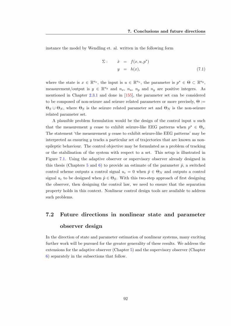
7. Conclusions and future directions
instance the model by Wendling et. al. written in the following form
Σ : x = f(x, u, p∗)
y = h(x), (7.1)
where the state is x ∈ Rnx , the input is u ∈ Rnu , the parameter is p∗ ∈ Θ ⊂ Rnp ,measurement/output is y ∈ Rny and nx, nu, np and ny are positive integers. As
mentioned in Chapter 2.3.1 and done in [155], the parameter set can be considered
to be composed of non-seizure and seizure related parameters or more precisely, Θ :=
ΘS ∪ ΘN , where ΘS is the seizure related parameter set and ΘN is the non-seizure
related parameter set.
A plausible problem formulation would be the design of the control input u such
that the measurement y cease to exhibit seizure-like EEG patterns when p? ∈ Θs.
The statement ‘the measurement y cease to exhibit seizure-like EEG patterns’ may be
interpreted as ensuring y tracks a particular set of trajectories that are known as non-
epileptic behaviour. The control objective may be formulated as a problem of tracking
or the stabilisation of the system with respect to a set. This setup is illustrated in
Figure 7.1. Using the adaptive observer or supervisory observer already designed in
this thesis (Chapters 5 and 6) to provide an estimate of the parameter p, a switched
control scheme outputs a control signal uc = 0 when p ∈ ΘN and outputs a control
signal uc to be designed when p ∈ ΘS . With this two-step approach of first designing
the observer, then designing the control law, we need to ensure that the separation
property holds in this context. Nonlinear control design tools are available to address
such problems.
7.2 Future directions in nonlinear state and parameter
observer design
In the direction of state and parameter estimation of nonlinear systems, many exciting
further work will be pursued for the greater generality of these results. We address the
extensions for the adaptive observer (Chapter 5) and the supervisory observer (Chapter
6) separately in the subsections that follow.
92

7. Conclusions and future directions
uModel input, Neural mass
model yModel output,
(EEG measurement) *, px
Adap.ve observer/ Supervisory observer
xState es6mate,
pParameter es6mate,
uModel input,
Prescribed model input, usually a Gaussian signal
Control input, uc
p∈ΘS
p∈ΘN
OR
Adap.ve Controller
Control input, uc = 0
Model output, y
Control input, uc
Model input, u
Proposed adap6ve control scheme to be designed
Figure 7.1: Proposed adaptive controller design for seizure abatement
7.2.1 Adaptive observer
We will work on extending the adaptive observer designed in Chapter 5 for the class of
nonlinear systems (5.1) to the following more general class of nonlinear systems
x0 = A0x0 + φ0(y)p?
x1 = A1x1 + φ1(x0, u)p?
x2 = A2x2 + φ2(x0, x1, u)p?
...
xn = Anxn + φn(x0, x1, . . . , xn−1, u)p?
y = C1x1 + C2x2 + · · ·+ Cnxn, (7.2)
where the states are xi ∈ Rni for i ∈ {0, . . . , n}, the parameter vector is p? ∈ Rnp , the
measurement is y ∈ Rny and the input is u ∈ Rnu . The nonlinear terms φ0 : R →Rn0 ×Rnp and φi : Rn0 × · · ·×Rni−1 ×Rnu → Rni ×Rnp , for i ∈ {1, . . . , n} are globally
Lipschitz. The matrices A0, . . . , An are Hurwitz.
This extension widens the class of systems considered by also including the model
by Wendling et al [155] described in Chapter 2.3.1. The available work in [46] applies
to a class of systems very similar to (7.2), but the issue arises in the linear part and
the output that is not of the same form as (7.2). Hence, future work entails addressing
93

7. Conclusions and future directions
this problem.
Another aspect that needs to be addressed is the robustness of the adaptive ob-
servers with respect to disturbances and uncertainties. We may perform a posteriori
analysis or re-design the observer such that the desired robustness properties are ob-
tained. This is essential for its practical applicability in realistic scenarios.
7.2.2 Supervisory observer
There is scope for much future research in supervisory estimation. In the results pre-
sented in Chapter 6, we have limited ourselves to considering constant plant parameters
p?. The conclusions of Theorem 7 may also be modified to for the case of slowly-varying
parameters p? using results for slowly-varying systems (see [86, Chapter 9.6]).
The robustness of the setup with respect to unmodelled dynamics and disturbances
in measured output y and input u remains to be investigated. This robustness prop-
erty is useful for the implementation of the supervisory observer in a practical setting
and will also form the basis for investigating other forms of disturbances in measured
output y, for example sampled and quantised measurements. This will have practical
applications, for instance when y is acquired by a digital device, such as in the case of
an implanted seizure control device or when y is transmitted over a limited capacity
channel.
Further work will also be done in obtaining conditions where the Assumption 18
(PE) is guaranteed. Under certain conditions, an input u may be designed with the
properties in [112, Chapter 6] for linear systems and [118] for nonlinear systems such
that Assumption 18 holds.
One drawback of the supervisory observer is the potentially high computation
needed for estimation as a result of the high number of parameter set sampling required
to obtain desirable ultimate bounds of the state and parameter estimation errors. This
is prohibitive when implemented with a high dimensional model, such as in the scale
of the full brain, instead of a local region of the cerebral cortex. Furthermore, if the
computations are to be executed by an implantable device, the high power consump-
tion due to the large number of computations is undesirable. Nevertheless, if prior
information about the plant’s parameter is available (e.g. the probability distribution
of the plant’s parameter in the set), then computational complexity may be reduced
by sampling efficiently according to the information available.
94

7. Conclusions and future directions
7.3 Concluding remarks: E tenebris in lucem
Control theoretic approaches to answering questions in neuroscience are still in its in-
fancy. This thesis presents some methodologies for estimating neural activity from
measurements such as the EEG. We hope that this endeavour will aid in better under-
standing of the human brain that eventually translates to useful medical solutions in
anticipating and controlling seizures caused by neurological disorders.
95

Appendix A: Mathematical
preliminaries
This appendix provides important tools used in the design of nonlinear observers and
for analysing the stability of systems in this thesis. A variety of references were used
to compile this appendix, the most important one is the textbook by H. Khalil [86].
Consider the following ordinary differential equation
x = f(x, t), (A.3)
where the vector x(t) ∈ Rnx is the state for every t ≥ t0 ≥ 0. The solution of (A.3)
with initial condition x(t0) is denoted x(t, x(t0)). The short hand notation x(t) will be
used instead where there is no ambiguity.
A model of a physical system such as a region of the human brain can only make
sense if x(t) exists, for all t ≥ t0 ≥ 0. This system is said to be forward complete [96].
For this to be true and for x(t) to be unique for all t ≥ t0 ≥ 0, f is assumed to satisfy
the following properties, for all initial conditions x(t0) ∈ B∆x ⊂ Rnx :
• there exists L > 0 such that
|f(t, x)− f(t, y)| ≤ L|x− y|, ∀(x, y, t) ∈ B∆x ×B∆x × R≥0. (A.4)
• f(t, x) is piecewise continuous in t and continuous in x.
The first condition is known as the Lipschitz property of the function f with Lipschitz
constant L.
An equilibrium point xe ∈ Rn of (A.3) is obtained by solving f(t, xe) = 0, for all
96

Appendix A: Mathematical preliminaries
t ≥ t0. A non-zero equilibrium point can always be translated to the origin, which gives
the following stability notions in terms of the origin xe = 0 as the equilibrium point:
Definition 2 (Stability notions). The origin xe = 0 of (A.3) is
• stable if, for each ε > 0, there is a δ = δ(ε, t0) > 0 such that
|x(t0)| ≤ δ =⇒ |x(t)| < ε, ∀t ≥ t0 ≥ 0. (A.5)
• uniformly stable (US) if, for each ε > 0, there is a δ = δ(ε) > 0 independent of
t0, such that (A.5) is satisfied.
• unstable if it is not stable.
• asymptotically stable if it is stable and there is a positive constant c = c(t0) such
that x(t)→ 0 as t→∞, for all |x(t0)| < c.
• uniformly asymptotically stable (UAS) if it is US and there is a positive constant
c independent of t0, such that for each η > 0, there is a T = T (η) > 0 such that
|x(t)| < η,∀t ≥ t0 + T (η), ∀|x(t0)| < c. (A.6)
• globally uniformly asymptotically stable (UGAS) if it is US, δ(ε) satisfies
limt→∞ δ(ε) =∞ and for η, c > 0, there is a T = T (η, c) > 0 such that
|x(t)| < η, ∀t ≥ t0 + T (η, c), ∀|x(t0)| < c. (A.7)
The ε−δ definition of different stability notions can be made more transparent using
comparison functions, i.e. class K functions and class KL functions in the following
lemma. We state this for the definitions of US and UAS as well as a special case of
UAS.
97

Appendix A: Mathematical preliminaries
Lemma 2 (Lemma 4.5 and Definition 4.5 in [86]). The equilibrium point xe = 0 of
(A.3) is
• US if and only if there is a class K function α and a positive constant c indepen-
dent of t0 such that
|x(t)| ≤ α(|x(t0)|), ∀t ≥ t0 ≥ 0, ∀|x(t0)| < c. (A.8)
• UAS if and only if there is a class KL function β and a positive constant c,
independent of t0 such that
|x(t)| ≤ β(|x(t0)|, t− t0), ∀t ≥ t0 ≥ 0, ∀|x(t0)| < c. (A.9)
• globally UAS (GUAS) if and only if inequality (A.9) is satisfied for any initial
state x(t0).
• exponentially stable if there exists a positive constant k such that the class KL
function β in (A.9) takes the form β(r, s) = kr exp(−λs).
98

Appendix B: Proofs
B.1 Proof of Theorem 1
We will do all proofs for the model by Wendling et al. described in Section 2.3.1,
which is the most general model that encompasses the models by Stam et al. and
Jansen et al. described in Sections 2.3.3 and 2.3.2 respectively. The proof for all other
models can be done by first identifying the cascade structure of the observation error
system, then showing that the subsystems satisfy certain properties to conclude the
global exponential stability of the whole observation error system. This is performed
in a similar fashion in the proof for the Wendling et al. model that follows.
From (3.1), (3.2), the dynamics of the state estimation error x := x− x is:
˙x = Ax+G(γ(Hx)− γ(Hx+KCx)) + LCx. (B.10)
The main idea is to consider the estimation error system (B.10) as the nominal error
system (B.10) with L = 0 and K = 0 perturbed by the terms Gγ(Hx) − Gγ(Hx +
K(Cx − y)) + LCx. As such, in Lemma 3, we build a Lyapunov function W for the
nominal error system. Next, using W as a candidate Lyapunov function for (B.10), we
obtain a bound for observer matrices K and L such that x = 0 is global exponential
stable (GES) [85, Definition 4.5].
Lemma 3. Consider the system (B.10). There exists a continuously differentiable
W : Rn → R such that the following holds, for all x ∈ Rn:
k1|x|2 ≤ W (x) ≤ k2|x|2,∣∣∣∂W (x)∂x
∣∣∣ ≤ k4|x|,
99

Appendix B.1: Proof of Theorem 1
and along solutions to system (B.10) with L = 0 and K = 0:
W (x) ≤ −k3|x|2, (B.11)
where k1, k2, k3 and k4 are strictly positive constants.
Proof. The nominal estimation error system (B.10) with L = 0 and K = 0 is
˙x = Ax+G(γ(Hx)− γ(Hx)). (B.12)
First note that system (3.1) has solutions that are defined for all time due to the
global Lipschitz property of function S and the fact that input u ∈ L∞ [85, Theorem
3.2]. In view of the same arguments, the solutions of system (3.2) (with y and u from
system (3.1)) are also well-defined and exist for all time. Consequently, we have that
(B.12) have solutions that are defined for all time.
We can decompose system (B.12) into 7 subsystems Σe1 to Σe7:
Σe1 : ˙x1 = A1x1 + φ1(x41)− φ1(x41)
Σe2 : ˙x2 = A2x2 + φ2(x51)− φ2(x51)
Σe3 : ˙x3 = A3x3 + φ3(x61, x71)− φ3(x61, x71)
Σe4 : ˙x4 = A4x4
Σe5 : ˙x5 = A5x5
Σe6 : ˙x6 = A6x6
Σe7 : ˙x7 = A7x7 + φ7(x51)− φ7(x51),
(B.13)
where xi := ( xi1, xi2 ) = ( xi1 − xi1, xi2 − xi2 ) ∈ R2 for i = {1, . . . , 7}. φ1(x41) =(0, θAaC2S2(x41)
), φ2(x51) =
(0, θBbC4S2(x51)
), φ3(x61, x71) =
(0, θGgC7S2(x61 −
x71)), φ7(x51) = (0, θBbC6S2(x51)). Matrices A1, . . . A7 are as defined in Section 2.4
100

Appendix B.1: Proof of Theorem 1
and have eigenvalues with strictly negative real parts.
We note that subsystem Σe1 is in cascade with Σe4, subsystems Σe2 and Σe7 are in
cascade with subsystem Σe5, and subsystem Σe3 is in cascade with Σe6 and Σe7. Using
this cascade structure, we show that the overall system (B.12) is GES by constructing
the desired Lyapunov function W from the Lyapunov functions of each subsystems Vi.
We consider Lyapunov functions V1, . . . , V7 for each subsystem Σe1 to Σe7 of the
form:
Vi = xTi Pixi for i ∈ {1, . . . , 7},
where P Ti = Pi > 0 satisfies the Lyapunov equation PiAi + ATi Pi = −I. This is
always possible as the eigenvalues of Ai have strictly negative real parts, in view of
[85, Theorem 4.6]. We will show that each subsystem Σei is input-to-state stable (ISS)
using Vi [135].
For subsystems Σe4, Σe5 and Σe6, taking the derivative of Vi = xTi Pixi along solu-
tions of Σei for i ∈ {4, 5, 6}, we obtain:
Vi ≤ −|xi|2 ≤ −1
2|xi|2.
Next, we show that V1 is an ISS-Lyapunov function [135] for subsystem Σe1 w.r.t
e4. Taking the derivative of V1 = xT1 P1x1 along the solutions of Σe1, we obtain:
V1 = xT1 (P1A1 +AT1 P1)x1 + 2xT1 P1(φ1(x41)− φ1(x41)).
Since the function S2 is globally Lipschitz with constant ρ2 from (2.4), we have that:
|φ1(x41)− φ1(x41)| ≤ θAaC2ρ2|x41 − x41| ≤ ρe1|x4|,
101

Appendix B.1: Proof of Theorem 1
where ρe1 = θAaC2ρ2. Therefore,
V1 ≤ −|x1|2 + 2|x1||P1|ρe1|x4|.
Recalling that ξχ ≤ 12ξ
2 + 12χ
2, for any ξ, χ ∈ R and letting ξ = 2|P1|ρe1|x4| and
χ = |x1|, we obtain the following:
V1 ≤ −|x1|2 +1
2|x1|2 + 2|P1|2ρ2
e1|x4|2
≤ −1
2|x1|2 + 2|P1|2ρ2
e1|x4|2.
With similar arguments for the remaining systems, along the solutions of Σei, for
i ∈ {2, 3, 7}:
Vi ≤ −1
2|xi|2 + γi|µi|2,
where µ1 = x4, µ2 = x5, µ3 = (x6, x7), µ7 = x5 and γi = 2|Pi|2ρ2ei where ρe2 = θBbC4ρ2,
ρe3 = θGgC7ρ2 and ρe7 = θBbC6ρ2.
The composite Lyapunov function for the overall system (B.13) W is constructed
using the Lyapunov function for each subsystem Vi [134]. We consider the candidate
Lyapunov function that is positive definite and radially unbounded:
W = a1V1 + a2V2 + a3V3 + V4 + V5 + V6 + a7V7, (B.14)
for a1, a2, a3, a7 > 0, which are determined below.
102

Appendix B.1: Proof of Theorem 1
The derivative of (B.14) along the solution of the overall error system (B.13) is
W ≤ −a11
2|x1|2 + a1γ1|x4|2 − a2
1
2|x2|2
+a2γ2|x5|2 − a31
2|x3|2 + a3γ3(|x6|2 + |x7|2)
−1
2|x4|2 −
1
2|x5|2 −
1
2|x6|2 − a7
1
2|x7|2 + a7γ7|x5|2.
By taking 0 < a1 <1
2γ1, 0 < a2 <
1γ2
(12 − a7γ7
), 0 < a3 <
12γ3
and a7 > 2a3γ3, we
obtain
W ≤ − 1
8γ1|x1|2 −
1
2γ2
(1
2− γ7
)|x2|2 −
1
8γ3|x3|2
−1
2|x4|2 −
1
2|x5|2 −
1
2|x6|2 −
1
4|x7|2. (B.15)
By letting P = diag(a1P1, a2P2, a3P3, P4, P5, P6, a7P7) as well as denoting λmin(P )
and λmax(P ) as the maximum and minimum eigenvalues of P respectively, we have
shown that (B.11) is fulfilled with k1 = λmin(P ) > 0, k2 = λmax(P ) > 0, k3 =
min{ 18γ1, 1
2γ2
(12 − γ7
), 1
8γ3, 1
4} > 0 and k4 = 2|P | > 0.
The derivative of W along the solutions to (B.10) is:
W =∂W
∂x
(Ax+G
(γ(Hx)− γ(Hx+KCx)
)+ LCx
),
=∂W
∂x
(Ax+Gγ(Hx)−Gγ(Hx)︸ ︷︷ ︸
nominal estimation error system (B.12)
+Gγ(Hx)−Gγ(Hx+KCx) + LCx︸ ︷︷ ︸perturbation terms
)
From Lemma 3:
W ≤ −k3|x|2 +∂W
∂xG(γ(Hx)− γ(Hx+KCx)) +
∂W
∂xLCx.
As γ is globally Lipschitz, |γ(Hx)− γ(Hx+KCx)| ≤ ρ|KCx| ≤ ρ|K||C||x|. From
103

B.2: Proof of Theorem 2
(B.11):
W ≤ −k3|x|2 +
∣∣∣∣∂W∂x∣∣∣∣ |G|ρ|K||C||x|+ ∣∣∣∣∂W∂x
∣∣∣∣ |L||C||x|≤ −k3|x|2 + k4|C||x|2(ρ|G||K|+ |L|),
where k3 and k4 are constructed in Lemma 3.
Therefore, if K and L satisfy the following condition:
ρ|K||G|+ |L| <k3
k4|C|,
then
W ≤ −k3|x|2,
where k3 = k3 − k4|C|(ρ|G||K|+ |L|) > 0.
Therefore, the origin of the estimation error system (B.10) is GES according to [85,
Definition 4.5], i.e. for all t ≥ 0,
|x(t)| ≤ k exp(−λt)|x(0)| ∀x(0) ∈ Rn,
for k, λ > 0. 2
B.2 Proof of Theorem 2
The proof that follows is performed for the Wendling at. al. model, where the models
by Stam et al. as well as Jansen and Rit can be derived from. The proof for these
models can be performed in a similar fashion.
From (3.5) and (3.6), the perturbed error system is:
˙x = Ax+G(p? + εp)γ(Hx)−G(p?)γ(Hx+K
(Cx− (y + εy)
))−L(Cx− (y + εy)) + σ(u, y, p? + εp)− σ(u+ εu, y + εy, p
?) + εsys
= (A+ LC)x+ Ψ(x, x)︸ ︷︷ ︸nominal system (B.10) from Theorem 1
+ Ψε(x, x, εy, εu, εp, εsys)︸ ︷︷ ︸perturbation terms
, (B.16)
104

B.2: Proof of Theorem 2
where K = (κ1, . . . , κm),
Ψ =(
0, θAaC2
(S2(x41)− S2(x41 − κ1Cx)
), 0, θBbC4
(S2(x51)− S2(x51 − κ2Cx
), 0,
θGgC7
(S2(x61−x71)−S2(x61−x71−κ3Cx)
), 0, 0, 0, 0, 0, 0, 0, θBbC6
(S2(x51)−S2(x51−
κ2Cx)))
and
Ψε =(
0, θAaC2
(S2(x41 − κ1Cx) − S2(x41 − κ1Cx − εy)
)+ aC2S2(x41)εp + auεp +
θAaεu, 0, θBbC4
(S2(x51 − κ2Cx)− S2(x51 − κ2Cx− εy)
)+ bC4S2(x51)εp, 0,
θGgC7
(S2(x61 − x71 − κ3Cx)− S2(x61 − x71 − κ3Cx− εy)
)+ gC7S2(x61 − x71)εp, 0,
θAaC1
(S2(y)− S2(y + εy)
)+ aC1S2(y)εp, θAaC3
(S2(y)− S2(y + εy)
)+ aC3S2(y)εθ, 0,
θAaC5
(S2(y)− S2(y+ εy)
)+ aC5S2(y)εp, 0, θBbC6
(S2(x51− κ2Cx)− S2(x51− κ2Cx−
εy))
+ bC6S2(x51)εp
)+ εsys.
We will show that the solutions of the error system (B.16) is input-to-state stable
(ISS) [133] with respect to the uncertainties εy, εu, εp and εsys. For this purpose, we
use function W as defined in (B.14).
The derivative of W along the solutions of (B.16) is:
W =∂W
∂x
((A+ LC)x+ Ψ(x, x)
)+∂W
∂xΨε(x, x, εy, εu, εp, εsys).
From Theorem 1, there exists k3, k4 > 0 such that:
W ≤ −k3|x|2 + k4|x||Ψε|.
Using the fact that the function S2 is globally Lipschitz with Lipschitz constant ρ2 and
S2(z) ≤ α2 for any z ∈ R as defined in (2.4), we obtain:
W ≤ −k3|x|2 + k4|x|(σy(|εy|) + σp(|εp|) + σu(|εu|) + |εsys|
)where σy(|εy|) =
(|(θAaC2ρ, θBbC4ρ, θGgC7ρ, θAaC1ρ, θAaC3ρ, θAaC5ρ, θBbC6ρ)| +
|L|)|εy|, σu(|εu|) = θAa|εu| and σp(|εp|) = |
((aC2α+ a‖u‖[0,t])|εp|, bC4α|εp|, gC7α|εp|,
aC1α|εp|, aC3α|εp|, aC5α|εp|, bC6α|εp|)|.
Therefore, if
|x| > 2k4
k3
(σy(|εy|) + σu(|εu|) + σp(|εp|) + |εsys|
),
105

Appendix B.3: Proof of Theorem 3
then
W ≤ −1
2k3|x|2. (B.17)
From (B.17), [85, (4.49) of Theorem 4.19] is fulfilled and [85, (4.48) of Theorem
4.19] is satisfied with α1 = k1 and α2 = k2, where k1 and k2 are from Lemma 3 in B.1.
Therefore, we can conclude that the error system (B.16) is ISS with respect to εy, εu,
εp and εsys with gains γy(s) = k2k1
2k4k3σy(s), γθ(s) = k2
k12k4k3σp(s), γu(s) = k2
k12k4k3σu(s) and
γsys(s) = k2k1
2k4k3.s, for s ≥ 0 and γy(0) = γθ(0) = γu(0) = γsys(0) = 0. Here, we have
shown it for the model by Wendling et al. [155], but similar arguments apply to all
other models considered in Chapter 2. 2
B.3 Proof of Theorem 3
Let V (x) = xTPx, its derivative along the solutions to (4.4) is:
V =xT(P (A+ LC) + (A+ LC)TP
)x+ 2xTPG(p?)δ(t)η
=
[x
δ(t)η
]T [(A+ LC)TP + P (A+ LC) PG(p?)
G(p?)TP 0
][x
δ(t)η
].
According to (4.5),
V ≤[
x
δ(t)η
]T[ −νI −(H +KC)TΛ
−Λ(H +KC) 2Λdiag( 1b1, . . . , 1
bm)
][x
δ(t)η
]
= −νxT x− 2ηT δ(t)Λ(H +KC)x+ 2ηT δ(t)Λdiag
(1
b1, . . . ,
1
bm
)δ(t)η.
Recall that η = v − w = (H + KC)x and since Λ and δ are diagonal, Λ = ΛT ,
δ(t) = δ(t)T and Λδ(t) = δ(t)Λ,
V ≤ −νxT x−2ηT δ(t)Λη+2ηT δ(t)Λdiag
(1
b1, . . . ,
1
bm
)δ(t)η
= −νxT x−2ηT(δ(t)Λ−δ(t)Λdiag
(1
b1, . . . ,
1
bm
)δ(t)
)η.
106

Appendix B.4: Proof of Theorem 4
If we examine the last term component-wise, we obtain:
δi(t)λi − δi(t)λib−1i δi(t) = δi(t)λi(1− b−1
i δi(t)).
From Assumption 9 and (4.3), we know that 1− b−1i δi(t) > 0, hence,
(δ(t)Λ− δ(t)Λdiag
(1
b1, . . . ,
1
bm
)δ(t)
)≥ 0.
We obtain V ≤ −νxT x. By [85, Theorem 4.10], we deduce that (4.6) holds. 2
B.4 Proof of Theorem 4
From (4.7) and (4.8), the observation error system is as follows:
˙x = (A+ LC)x+ Lεy + σ(u, y)− σ(u+ εu, y + εy)
+Gγ(Hx)−Gγ(Hx+K
(Cx−(y+εy)
))+εsys. (B.18)
By introducing ±Gγ(Hx + K
(Cx − y
))to (B.18), we obtain an observation error
system that can be considered as the nominal system (4.4) perturbed by a term that
depends on εy, εu and εsys as shown below:
˙x = (A+ LC)x+G(γ(Hx)− γ(Hx+K
(Cx− y)
))︸ ︷︷ ︸nominal system (4.4)
+ Ψε(x, x, εy, εu, εsys)︸ ︷︷ ︸perturbation terms
, (B.19)
where Ψε = Gγ(Hx + K(Cx − y)
)− Gγ
(Hx + K
(Cx − (y + εy)
))+ Lεy + σ(y, u) −
σ(u+ εu, y + εy) + εsys.
Let V (e) = xTPx, by following the same arguments as in the proof of Theorem 3,
107

Appendix B.5: Proof of Proposition 1
along solutions to (B.19), we obtain
V ≤ −νxT x+ 2xTPΨε. (B.20)
The perturbation Ψε can be bounded as follows:
|Ψε| ≤ σy|εy|+ σu|εu|+ |εsys|, (B.21)
where σy = |G||diag(b1, . . . , bm)||K|+|L|+|diag(b1, . . . , bn)| and σu = |diag(b1, . . . , bn)|.From (B.20) and the bound on the perturbation terms (B.21):
V ≤ −ν|x|2 + 2|x||P |(σy|εy|+ σu|εu|+ |εsys|
).
Consequently, if |x| > 4|P |ν (σy|εy| + σu|εu| + |εsys|
), then V ≤ −ν
2 |x|2. By [85, Theo-
rem 4.19], (4.9) is satisfied with γy = λmax(P )λmin(P )
4|P |ν σy, γu = λmax(P )
λmin(P )4|P |ν σu and γεsys =
λmax(P )λmin(P )
4|P |ν . 2
B.5 Proof of Proposition 1
Let p? ∈ Θ, the perturbed model (4.10) has solutions for all t ≥ 0 as γ and σ are
globally Lipschitz, the input u and the uncertainty εp are in L∞ [85, Theorem 3.2]. We
can write the perturbed model (4.10) in the form of (4.7) with εsys = G(p?+εp)γ(Hx)−G(p?)γ(Hx)+ σ(u, y, p?+ εp)− σ(y, u, p?). As Assumptions 9-10 are satisfied, we apply
Theorem 4 and obtain the following:
|x(t)| ≤ k exp(−βt)|x(0)|+ γy‖εy‖[0,t] + γu‖εu‖[0,t] + γεsys‖εsys‖[0,t]. (B.22)
Noting that the uncertainty is εsys = G(p? + εp)γ(Hx)−G(p?)γ(Hx) + σ(u, y, p? +
εp) − σ(u, y, p?), we use the fact that γ and σ are globally Lipschitz and bounded to
show that εp satisfies the following
|εp| ≤ σp|εp|, (B.23)
where σp = |(aC2α, bC4α)|+|(a‖u‖[0,∞], aC3α, aC1α)|, recalling that ‖u‖[0,∞] ≤ 320mV
108

Appendix B.6: Proof of Theorem 5
[74, Section 3.1]. We deduce from (B.22) and (B.23) that (4.19) is satisfied with γp =
σpγεsys . 2
B.6 Proof of Theorem 5
Firstly, x(t) exists for all t ≥ 0 by Theorem 3.2 of [86], because γ is globally Lipschitz
and u is a continuous function that is defined for all t ≥ 0. We now show that the obser-
vation error system satisfies property (4.24) by taking the derivative of the Lyapunov
function V (x) = xTPx along the solutions of (4.22), where χ = (x, δ(t)η, w, d):
V (x) = xT(P (A+ LC) + (A+ LC)TP
)x+ 2xTPGδ(t)η
−2xTPLDw + 2xTPBd
= χT
P (A+ LC) + (A+ LC)TP PG −PLD PB
? 0 0 0
? ? 0 0
? ? ? 0
χ.
Applying (4.25), we obtain:
V (x) ≤ χT
−I −(H +KC)TM 0 0
? −E(M) MKD 0
? ? µwI 0
? ? ? µdI
χ= −|x|2 − 2xT (H +KC)TMδ(t)η + 2ηT δ(t)MKDw
−ηT δ(t)TE(M)δ(t)η + µw|w|2 + µd|d|2.
Recall that η := z−v = (H+KC)x−KDw, hence (H+KC)x = η+KDw. Therefore,
V (x) ≤ −|x|2 − 2(η +KDw)TMδ(t)η + 2ηT δ(t)MKDw
−ηT δ(t)TE(M)δ(t)η + µw|w|2 + µd|d|2.
109
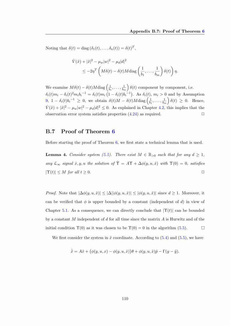
Appendix B.7: Proof of Theorem 6
Noting that δ(t) = diag (δ1(t), . . . , δn(t)) = δ(t)T ,
V (x) + |x|2 − µw|w|2 − µd|d|2
≤ −2ηT(Mδ(t)− δ(t)Mdiag
(1
b1, . . . ,
1
bm
)δ(t)
)η.
We examine Mδ(t)− δ(t)Mdiag(
1b1, . . . , 1
bm
)δ(t) component by component, i.e.
δi(t)mi − δi(t)2mibi−1 = δi(t)mi
(1− δi(t)bi−1
). As δi(t), mi > 0 and by Assumption
9, 1 − δi(t)bi−1 ≥ 0, we obtain δ(t)M − δ(t)Mdiag
(1b1, . . . , 1
bm
)δ(t) ≥ 0. Hence,
V (x) + |x|2 − µw|w|2 − µd|d|2 ≤ 0. As explained in Chapter 4.2, this implies that the
observation error system satisfies properties (4.24) as required. 2
B.7 Proof of Theorem 6
Before starting the proof of Theorem 6, we first state a technical lemma that is used.
Lemma 4. Consider system (5.5). There exist M ∈ R>0 such that for any d ≥ 1,
any L∞ signal x, y, u the solution of Υ = AΥ + ∆φ(y, u, x) with Υ(0) = 0, satisfies
|Υ(t)| ≤M for all t ≥ 0. 2
Proof. Note that |∆φ(y, u, x)| ≤ |∆||φ(y, u, x)| ≤ |φ(y, u, x)| since d ≥ 1. Moreover, it
can be verified that φ is upper bounded by a constant (independent of d) in view of
Chapter 5.1. As a consequence, we can directly conclude that |Υ(t)| can be bounded
by a constant M independent of d for all time since the matrix A is Hurwitz and of the
initial condition Υ(0) as it was chosen to be Υ(0) = 0 in the algorithm (5.5).
We first consider the system in x coordinate. According to (5.4) and (5.5), we have
˙x = Ax+(φ(y, u, x)− φ(y, u, x)
)θ + φ(y, u, x)p− Γ(y − y).
110

Appendix B.7: Proof of Theorem 6
We scale the error x as such x := ∆x. Noting that ∆A∆−1 = A:
˙x = Ax+ ∆(φ(y, u, x)− φ(y, u, x)
)p? + ∆φ(y, u, x)p−∆Γ(y − y). (B.24)
We now proceed to a dynamical change of coordinates by introducing η as follows
which was as proposed in [160]:
η := x−Υp.
Noting that C∆−1 = dC, the dynamics of variables η and p are given by:
{η = Aη + ∆
(φ(y, u, x)− φ(y, u, x)
)p?
˙p = −dPΥTCTC(η + Υp).(B.25)
We note that, contrary to [160], we have not obtained a nice cascade system since
the η-system also depends on x and x. In the following, we will invoke small-gain
type arguments to conclude the stability of system (B.25). We consider the Lyapunov-
type functions V1(η) = ηTSη and V2(p, P ) = pTP−1p where S is a real symmetric
positive definitive matrix such that ATS + SA = −I (such a matrix always exists
according to Theorem 4.6 in [86] since A is Hurwitz). It can be noted that V2 satisfies
λ1|p|2 ≤ V2(p, P ) ≤ λ2|p|2 where λ1, λ2 are independent of d for d ≥ 1 according to
[162, Lemma 1], which will be useful for our purpose. We first consider V1. Along
solutions to (B.25), we have:
V1(t) = −|η|2 + 2ηTS∆(φ(y, u, x)− φ(y, u, x)
)p?. (B.26)
Noting that φ(x, y, u) =(φ0(y), φ1(x0, u)
), so φ(x, y, u) − φ(x, y, u) = (0, φ1(x0, u) −
φ1(x0, u)). As a consequence,
∆(φ(y, u, x)− φ(y, u, x)) =(0, 1
d(φ1(x0, u)− φ1(x0, u)))
from which we deduce in (B.26):
V1(t) ≤ −|η|2 + 2|η||S||p?||∆(φ(x0, u)− φ(x0, u)
)|
≤ −|η|2 + 2|η||S||p?|(
1d |φ1(x0, u)− φ1(x0, u)|
).
111

Appendix B.7: Proof of Theorem 6
By assumption, φ1 is globally Lipschitz with a constant that we denote L1 > 0, thus
|φ1(x0, u) − φ1(x0, u)| ≤ L1|x0|. Note also that the scaling induced by the matrix ∆
does not affect the x0 part of the estimation error x, so that we have x0 = x0. As a
consequence,
V1(t) ≤ −|η|2 + 2d |η||S||p?|L1|x0|
≤ −|η|2 + 2d |η||S||p?|L1(|η|+ |Υp|)
= (−1 + 2d |S||p?|L1)|η|2 + 2
d |η||S||p?|L1|Υp|.(B.27)
We define
d? := max{1, 4L1|p?||S|}. (B.28)
Choose d such that d ≥ d?, so that −1 + 2d |S||p?|L1 < −1
2 , in that way: V1(t) ≤−1
2 |η|2 + 2d |S|L1|p?||η||Υp|. According to Lemma 4, we always have |Υ| ≤M , therefore:
V1(t) ≤ −12 |η|2 + 2
d |S||θ|L1M |η||p|, from which we deduce, by invoking the fact that S
and P−1 are symmetric positive definite with lower and upper bounds independent of
d (see [162, Lemma 1]), that there exists σ1, σ2 ∈ R>0 independent of d such that:
V1(t) ≤ −σ1V1 + 1dσ2
√V1
√V2
= −σ12 V1 − σ1
2 V1 + 1dσ2
√V1
√V2,
(B.29)
as a consequence, noting that 1dσ2
√V1
√V2 ≤ σ1
2 V1 can be written as 1d2σ2
2V2 ≤ σ214 V1:
(σd2V2 ≤ V1
)⇒
(V1(t) ≤ −σ1
2 V1
), (B.30)
with σ = 4(σ2σ1
)2. That is all we need so far concerning V1. Consider V2, along solutions
to (5.5) and (B.25), the following is satisfied (recall that V2(p, P ) = pTP−1p):
V2(t) = −pTP−1PP−1p+ 2pTP−1 ˙p
= −dV2 − dpTΥTCTCΥp− 2dpTΥTCTCη,
since pTΥTCTCΥp ≥ 0, V2(t) ≤ −dV2 − 2dpTΥTCTCη. By invoking the same argu-
ments as after (B.29) and since Υ is bounded by M according to Lemma 4, there exists
γ ∈ R>0 independent of d such that |2dpTΥTCTCη| ≤ dγ√V1
√V2 so that:
V2(t) ≤ −dV2 + γd√V1
√V2
= −d2V2 − d
2V2 + γd√V1
√V2
112

Appendix B.7: Proof of Theorem 6
since γd√V1
√V2 ≤ d
2V2 is equivalent to γ2V1 ≤ 14V2, we deduce that:
(σV1 ≤ V2
)⇒
(V2(t) ≤ −d
2V2
), (B.31)
with σ = 4γ2. Following the proof of Theorem 3.1 in [76], we are going to define a
Lyapunov function for the system (B.25) based on V1 and V2. Let d be sufficiently large
such that σd2< σ−1 (i.e. such that the small gain condition is satisifed) and take χ > 0
such that:σd2< χ < σ−1. (B.32)
We introduce the candidate Lyapunov function, V = max{V1, χV2}. Function V is the
maximum of two continuously differentiable functions, therefore it is locally Lipschitz
and so differentiable almost everywhere according to Rademacher’s theorem. Along
solutions to (B.25), when V = V1 that means V1 ≥ χV2 ≥ σd2V2. (B.30) shows us
that V (t) ≤ −σ12 V (t) almost everywhere. Similarly, when V = χV2 that means V2 ≥
χ−1V1 ≥ σV1 so (B.31) shows us that V (t) ≤ −d2χV (t) almost everywhere. As a
consequence, we have that, almost everywhere: V (t) ≤ −min{σ12 , d2χ}V . Taking d ≥d? ≥ 1,
V (t) ≤ −min{σ12 , d2χ}V ≤ −min{σ12 , 12χ}V =: −λV.
Using the comparison principle (see Lemma 3.4 in [86]) and the fact that V is positive
definite and radially unbounded, we obtain:
|(η(t), p(t))| ≤ β(|(η(0), p(0))|, t
)∀t ≥ 0, (B.33)
where β ∈ KL. By the definition of x,
|(x, p)| = |(∆−1η + ∆−1Υp, p)|≤ d|(η + Υp, p)| ≤ d|η + Υp|+ d|p|≤ d|η|+ d(1 +M)|p| ≤ d(1 +M)|(η, p)|.
From (B.33) and η(0) = ∆x(0)−Υ(0)p(0). As Υ(0) = 0 by initialisation, we have that
η(0) = ∆x(0). Recalling that |∆| ≤ 1 (since d ≥ 1), hence |η(0)| ≤ |∆||x(0)| ≤ |x(0)|
113

Appendix B.8: Proof of Proposition 2
and we obtain:
|(x(t), p(t))| ≤ d(1 +M)β(|(η(0), p(0))|, t
)≤ d(1 +M)β
(|(x(0), p(0))|, t
).
Therefore, we obtain the desired property (5.8) with βd(s, t) = d(1 +M)β(s, t). 2
B.8 Proof of Proposition 2
We write the state error system (6.4), for all i ∈ {1, . . . , N} in the following form
ξ = Fi(ξ, %, p?, u, x)
η = H(ξ, x, %, p?). (B.34)
where ξ ∈ Rnx , % ∈ Rnp and η ∈ Rny . We denote the solution of system (B.34) at time
t with parameter error % as ξ(t, %), where we have omitted its dependance on its initial
condition x(0) and on its input u. Similarly, we denote the output of (B.34) as η(t, %).
Let W (t, %) :=∫ tt−Tf |η(s, %)|2ds. We show that W is continuous in %. First, since
the function f is continuously differentiable, % ∈ Θ, p? ∈ Θ, u ∈ M∆u and x ∈ BKx(by Assumption 16), Fi is locally Lipschitz in ξ, uniformly in %, p?, u and x by Lemma
2.3 of [85]. Hence, ξ(t, %) is continuous in t and % by Theorem 2.6 in [85]. As a
consequence, we deduce that η(t, %) is also continuous in % and t by using the fact
that H is continuous in view of Assumption 15. Thus, we have that ρ 7→ |η(t, ρ)| is
continuous in Θ. Moreover, |η(t, %)| ≤ φ(t), with φ(t) := max%∈Θ|η(t, %)|2 integrable on
[t−T, t] using the fact that Θ is a compact set. Hence, we deduce that W is continuous
in % on Θ, by using the dominated convergence theorem [14, Theorem 10.27].
So far, for any fixed t, W (t, %) ≥ 0 for all % by definition and we have established
that W (t, %) is continuous in %. Hence, we can lower bound the function W by a
positive definite and continuous function W in %. This allows us to apply Lemma
3.5 in [85] on W to obtain a class K function αy such that W (t, %) ≥ αy(|%|). Since,
W (t, %) ≥ W (t, %), (6.9) holds as desired. 2
114

Appendix B.9: Proof of Lemma 1
B.9 Proof of Lemma 1
We first prove in Claims 1 and 2 desirable properties of the state error systems (6.4) and
the monitoring signals µi, where i ∈ {1, . . . , N}. In Claim 1, the state error system (6.4)
is shown to be locally ISS (see [85, Definition 5.2]) with respect to the parameter error
pi. This property, along with Assumption 18, are the key ingredients that allow us to
show in Claim 2 that the monitoring signals are lower and upper bounded by functions
of the parameter error pi that are strictly increasing with |pi|. These properties allow
us to conclude the proof of Lemma 1. Claims 1 and 2 are also later used in the proof
of Theorem 7.
Claim 1. Consider the state error system (6.3) for i ∈ {1, . . . , N} under Assumptions
15-17. There exist constants k, λ > 0 such that for any ∆x, ∆x, ∆u > 0, there exists
a class K function γx such that for all (xi(0), x(0)) ∈ B∆x × B∆x, for all pi ∈ Θ and
for all u ∈M∆u, the corresponding solution satisfies
|xi(t)| ≤ k exp(−λt)|xi(0)|+ γx(|pi|), ∀t ≥ 0. (B.35)
2
Proof of Claim 1. For i ∈ {1, . . . , N}, by Assumption 17, the following holds for all
xi ∈ Rnx , x ∈ Rnx , u ∈ Rnu , p? ∈ Θ and pi ∈ Θ
a1|xi|2 ≤ Vi(xi) ≤ a2|xi|2, (B.36)
∂Vi∂xi
Fi(xi, pi, p?, u, x) ≤ −λ0Vi(xi) + γ(pi, x, u). (B.37)
Given ∆x, ∆u > 0, letKx > 0 be generated by Assumption 16 such that |x(t)| ≤ Kx,
for all t ≥ 0 and u ∈ M∆u . Since γ is a continuous function and γ(0, z, z) = 0, for all
z ∈ Rnx , z ∈ Rnu , we have that
γ1(pi) := max|x|≤Kx,|u|≤∆uγ(pi, x, u) is a continuous and positive definite function in
115

Appendix B.9: Proof of Lemma 1
pi. By Lemma 3.5 in [85], there exists a class K function γ such that for pi ∈ Θ
γ1(pi) ≤ γ(|pi|), (B.38)
as Θ is a compact set.
We use (B.36), (B.37) and (B.38) to obtain the following for all |x| ≤ Kx and
|u| ≤ ∆u
∂Vi∂xi
Fi(xi, pi, p?, u, x) ≤ −λ0Vi(xi) + γ(|pi|). (B.39)
By the comparison principle (Lemma 2.5 in [85]), for all (x(0), xi(0)) ∈ B∆x × B∆x ,
u ∈M∆u , the corresponding solutions of (B.39) are
Vi(xi(t)) ≤ exp(−λ0t)Vi(xi(0)) +1
λ0γ(|pi|), (B.40)
for t ∈ [0, tmax), where tmax ∈ R≥0 ∪∞ is the solution’s maximal time of existence. We
use (B.36) and the fact that for any a, b > 0,√a+ b ≤
√2a +
√2b to obtain (B.35)
for all t ∈ [0, tmax) as desired with k :=√
2a2a1
, λ := λ02 and γx(r) :=
√2
a1λ0
√γ(r). We
deduce from (B.40) that tmax =∞ by contradiction.
Claim 2. Consider the plant (6.1), the state error system (6.4) and the monitoring
signal (6.7), for i ∈ {1, . . . , N} under Assumptions 15-18. For any ∆x, ∆x, ∆u > 0,
there exist class K functions χ and χ and for any ε > 0, there exists a constant T =
T (∆x,∆x,∆u, ε) > 0, such that the monitoring signal µi in (6.7) satisfy the following
for all (x(0), xi(0)) ∈ B∆x ×B∆x, for some u ∈M∆u that satisfies Assumption 18, for
any p? ∈ Θ and for all pi ∈ Θ
χ(|pi|) + cµ ≤ µi(t) ≤ χ(|pi|) + ε+ cµ, ∀t ≥ T. (B.41)
2
116

Appendix B.9: Proof of Lemma 1
Proof of Claim 2. Given ∆x, ∆x, ∆u, ε > 0, we first construct the following from
Assumptions 15-18.
• Let constants k, λ > 0 and a class K function γx be generated from Claim 1. Given
that for i ∈ {1, . . . , N}, pi ∈ Θ, where Θ is a compact set, there exists Kp > 0
such that |pi| ≤ Kp. By Claim 1, the solutions of (6.4) satisfy the following for
all (xi(0), x(0)) ∈ B∆x ×B∆x , for all (p?, pi) ∈ Θ× Θ, for all u ∈M∆u and for all
t ≥ 0
|xi(t)| ≤ k exp(−λt)|xi(0)|+ γx(|pi|) ≤ k∆x + γx(Kp) =: Kx. (B.42)
• Since h is continuously differentiable in view of Assumption 15, h is locally Lips-
chitz. Therefore, there exist constants lx, lp > 0 such that for x ∈ BKx , xi ∈ BKx ,
and pi ∈ Θ, p? ∈ Θ, the following holds
|H(xi, x, pi, p?)−H(0, x, 0, p?)| = |H(xi, x, pi, p
?)|
= |h(xi + x, pi + p?)− h(x, p?)|
≤ lx|xi|+ lp|pi|, (B.43)
where H(0, x, 0, p?) = 0 in view of the definition of H in (6.4).
• Let λ > 0 come from (6.7) and given ε > 0, we choose εx, εµ > 0 sufficiently small
such that
εµ +4l2xε
2x
λ= ε. (B.44)
Let Tx > 0 be such that for all |x(0)| ≤ ∆x, |xi(0)| ≤ ∆x and u ∈M∆u
k exp(−λt)|xi(0)| ≤ εx, ∀t ≥ Tx. (B.45)
117
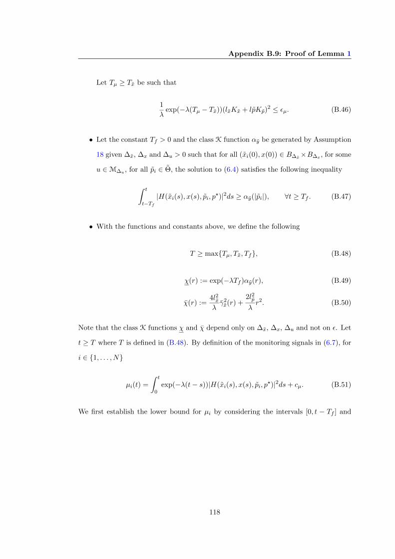
Appendix B.9: Proof of Lemma 1
Let Tµ ≥ Tx be such that
1
λexp(−λ(Tµ − Tx))(lxKx + lpKp)
2 ≤ εµ. (B.46)
• Let the constant Tf > 0 and the class K function αy be generated by Assumption
18 given ∆x, ∆x and ∆u > 0 such that for all (xi(0), x(0)) ∈ B∆x×B∆x , for some
u ∈M∆u , for all pi ∈ Θ, the solution to (6.4) satisfies the following inequality
∫ t
t−Tf|H(xi(s), x(s), pi, p
?)|2ds ≥ αy(|pi|), ∀t ≥ Tf . (B.47)
• With the functions and constants above, we define the following
T ≥ max{Tµ, Tx, Tf}, (B.48)
χ(r) := exp(−λTf )αy(r), (B.49)
χ(r) :=4l2xλγ2x(r) +
2l2pλr2. (B.50)
Note that the class K functions χ and χ depend only on ∆x, ∆x, ∆u and not on ε. Let
t ≥ T where T is defined in (B.48). By definition of the monitoring signals in (6.7), for
i ∈ {1, . . . , N}
µi(t) =
∫ t
0exp(−λ(t− s))|H(xi(s), x(s), pi, p
?)|2ds+ cµ. (B.51)
We first establish the lower bound for µi by considering the intervals [0, t − Tf ] and
118

Appendix B.9: Proof of Lemma 1
[t− Tf , t] to obtain
µi(t) =
∫ t−Tf
0exp(−λ(t− s))|H(xi(s), x(s), pi, p
?)|2ds
+
∫ t
t−Tfexp(−λ(t− s))|H(xi(s), x(s), pi, p
?)|2ds+ cµ
≥∫ t
t−Tfexp(−λ(t− s))|H(xi(s), x(s), pi, p
?)|2ds+ cµ. (B.52)
As s 7→ exp(λs) is strictly increasing, we obtain the following lower bound
µi(t) ≥ exp(−λTf )
∫ t
t−Tf|H(xi(s), x(s), pi, p
?)|2ds+ cµ. (B.53)
From (B.47), (B.49) and our choice of T , since t ≥ T ≥ Tf
µi(t) ≥ exp(−λTf )αy(|pi|) + cµ = χ(|pi|) + cµ. (B.54)
We now obtain the upper bound of µi by considering the integration intervals [0, Tx]
and [Tx, t], since t ≥ T ≥ Tx.
µi(t) =
∫ Tx
0exp(−λ(t− s))|H(xi(s), x(s), pi, p
?)|2ds
+
∫ t
Tx
exp(−λ(t− s))|H(xi(s), x(s), pi, p?)|2ds+ cµ. (B.55)
119

Appendix B.9: Proof of Lemma 1
Using (B.43) and the fact that for any a, b ≥ 0, (a+ b)2 ≤ 2a2 + 2b2, we obtain
µi(t) ≤1
λexp(−λ(t− Tx))
(sup
s∈[0,Tx]|H(xi(s), x(s), pi, p
?)|2)
+
∫ t
Tx
exp(−λ(t− s))(lx|xi(s)|+ lp|pi|
)2ds+ cµ
≤ 1
λexp(−λ(t− Tx))
(sup
s∈[0,Tx]|H(xi(s), x(s), pi, p
?)|2)
+
∫ t
Tx
exp(−λ(t− s))(
2l2x|xi(s)|2 + 2l2p|pi|2)ds+ cµ. (B.56)
We also have from Claim 1 and (B.45) that for all i ∈ {1, . . . , N}
|xi(t)| ≤ εx + γx(|pi|), ∀t ≥ Tx, (B.57)
which implies that, using the fact that for any a, b > 0, (a+ b)2 ≤ 2a2 + 2b2
|xi(t)|2 ≤ 2ε2x + 2γ2x(|pi|), ∀t ≥ Tx. (B.58)
Also, by (B.42) and (B.43), we obtain
sups∈[0,Tx]
|H(xi(s), x(s), pi, p?)|2 ≤ sup
s∈[0,Tx](lx|xi(s)|+ lp|pi|)2
= (lxKx + lpKp)2. (B.59)
Hence, from (B.56) and in view of (B.46), (B.58) and (B.59), we have the following for
t ≥ T ≥ Tµ ≥ Tx
µi(t) ≤ εµ + cµ +
∫ t
Tx
exp(−λ(t− s))(
4l2xε2x + 4l2xγ
2x(|pi|) + 2l2p|pi|2
)ds
= εµ + cµ +
(∫ t
Tx
exp(−λ(t− s))ds)(
4l2xε2x + 4l2xγ
2x(|pi|) + 2l2p|pi|2
).
(B.60)
120

Appendix B.9: Proof of Lemma 1
Note that∫ tTx
exp(−λ(t− s))ds = 1λ
(1− exp(−λ(t−Tx))
)and for t ≥ Tx, we have that∫ t
Txexp(−λ(t− s))ds ≤ 1
λ . Therefore, from (B.60), for t ≥ Tx
µi(t) ≤ εµ + cµ +4l2xε
2x
λ+
4l2xλγ2x(|pi|) +
2l2pλ|pi|2. (B.61)
By the definition of ε and χ in (B.44) and (B.50) respectively:
µi(t) ≤ ε+ χ(|pi|) + cµ. (B.62)
Therefore, from (B.54) and (B.62), we complete the proof.
We are now ready to prove Lemma 1. Given that the switching logic (6.12) is
scale-independent, the switching signal σ is not affected if the monitoring signal µi(t),
i ∈ {1, . . . , N} is replaced by its scaled version, for t ≥ 0
µi(t) := exp(λt)µi(t) = exp(λt)cµ +
∫ t
0exp(λs)|yi(s)|2ds. (B.63)
Note that the scaled monitoring signal µi has the following properties
1. µi(0) = cµ > 0.
2. µi(t) is non-decreasing.
The scaled monitoring signal µi is then used for analysis purposes in [67] and [95,
Chapter 6]. It has been shown in [151] that in the supervisory control of nonlinear
plants with disturbances, the scale independent hysteresis switching logic σ in (6.12)
satisfy dwell time conditions for bounded disturbances. We follow this approach in the
analysis that follows. By Lemma 4.2 in [151], we have that the number of switches in
the interval [0, t), Nσ(t, 0) satisfies the following
Nσ(t, 0) ≤ N +N
ln(1 + h)ln
(µl(t)
minq∈{1,...,N} µq(0)
)(B.64)
For an arbitrary ε, ∆x, ∆x, ∆u > 0, let a class K function χ and a constant
121

Appendix B.10: Proof of Theorem 7
T = T (∆x,∆x,∆u, ε) > 0 be generated by Claim 2. From Claim 2, for all % ∈ Θ,
(x(0), ξ(0)) ∈ B∆x × B∆x , for all u ∈ M∆u that satisfies Assumption 18 and for all
t ≥ Tµi(t) ≤ χ(|%|) + ε+ cµ. (B.65)
Hence, by definition (B.63)
µi(t) ≤ exp(λt)(χ(|%|) + ε+ cµ
). (B.66)
From (B.64), (B.66) and µi(0) = exp(λ0)cµ = cµ, we obtain the following for all t ≥ T
Nσ(t, 0) ≤ N +N
ln(1 + h)ln
exp(λt)(χ(|%|) + ε+ cµ
)exp(λ0)cµ
= N +
N
ln(1 + h)ln
(χ(|%|) + ε
cµ+ 1
)+
t(ln(1+h)λN
) . (B.67)
Recall from (6.13) that a switching signal σ satisfies average dwell time conditions. It
holds that
Nσ(t, 0) ≤ N0 +t
τa. (B.68)
Therefore, comparing (B.67) and (B.68) yields
τa = ln(1+h)λN , N0 = N + N
ln(1+h) ln(χ(|%|)+ε
cµ+ 1)≥ 1. (B.69)
Hence, from (B.69), we have shown that σ has an average dwell time by obtaining
(6.14) as desired. 2
B.10 Proof of Theorem 7
The proof of Theorem 7 uses Claims 1-2 from the proof of Lemma 1 (Appendix B.9).
They show properties of the state error systems (6.4) and the monitoring signals (6.7)
which enable us to complete the proof. The state estimation error system (6.17)
switches between the individual state estimation error systems (6.4) in a manner that
122

Appendix B.10: Proof of Theorem 7
does not affect the individual systems (6.4) as explained in Remark 8. Therefore,
|xσ(t)(t)| ≤ maxi∈{1,...,N}
|xi(t)|, ∀t ≥ 0. (B.70)
By Claim 1, for i ∈ {1, . . . , N}, for all xi(0) ∈ B∆x , pi ∈ Θ and u ∈ M∆u , the
corresponding solution of (6.4) satisfies
|xi(t)| ≤ k exp(−λt)|xi(0)|+ γx(|pi|). (B.71)
As pi ∈ Θ for i ∈ {1, . . . , N}, where Θ is a compact set, let the constant Kp > 0 be
such that |pi| ≤ Kp. We have from (B.71) and (B.77) that
|xi(t)| ≤ k∆x + γx(Kp) =: Kx, ∀t ≥ 0. (B.72)
Hence, we have that the solution of the switched state error system (6.17) satisfies
|xσ(t)(t)| ≤ Kx, ∀t ≥ 0. (B.73)
Hence, xσ(t)(t) cannot escape to infinity in finite time. Moreover, we have proved in
Lemma 1 that the switching logic σ satisfies average dwell time conditions. Therefore,
no Zeno behaviour can occur. Hence, xσ(t)(t) is defined for all t ≥ 0.
We now construct the core elements for the rest of the proof.
• Given ∆x, ∆x, ∆u > 0, we generate constants k, λ > 0 and a class K function γx
from Claim 1. Let ν1 > 0 be such that
ν1 ≤ γ−1x (νx), (B.74)
where νx > 0 is given.
• Let class K functions χ and χ be generated by Claim 2. Choose ε, h? > 0
sufficiently small be such that
1
1 + h?χ(min{νp, ν1})−
h?
1 + h?cµ − ε > 0, (B.75)
123

Appendix B.10: Proof of Theorem 7
where νp > 0 and cµ > 0 (from the monitoring signal (6.7)) are given and let
T > 0 be generated by Claim 2 given the chosen ε from (B.75). Let
δ? := χ−1
(1
1 + h?χ(min{νp, ν1})−
h?
1 + h?cµ − ε
). (B.76)
Note that δ? > 0 due to (B.75).
• As pi ∈ Θ for i ∈ {1, . . . , N}, where Θ is a compact set, let the constant Kp > 0
be such that |pi| ≤ Kp. We define
Kx := k∆x + γx(Kp). (B.77)
Let t ≥ 0. Recall that we denote the chosen monitoring signal at each time t as
µσ(t)(t). There are two possible scenarios: (i) µσ(t)(t) = minj∈{1,...,N} µj(t) and (ii)
µσ(t)(t) 6= minj∈{1,...,N} µj(t). We first consider case (ii), since case (i) immediately
follows as we will see. The switching condition of σ defined in (6.12) is not satisfied,
which means that for all q ∈ {1, . . . , N},
µq(t)(1 + h) ≥ µσ(t)(t). (B.78)
Consequently, by Claim 2, for all t ≥ T
(1 + h)(χ(|pq|) + ε+ cµ
)≥ χ(|pσ(t)(t)|) + cµ. (B.79)
As h ∈ (0, h?], (1 + h?)(χ(minq∈{1,...,N} |pq|
)+ ε+ cµ
)− cµ ≥ χ(|pσ(t)(t)|).
Since minq∈{1,...,N} |pq| ≤ δ?,
(1 + h?)(χ (δ?) + ε+ cµ
)− cµ ≥ χ(|pσ(t)(t)|). (B.80)
By the definition of δ? in (B.76), we obtain the following from (B.80)
χ−1(
(1 + h?)(χ(δ?) + ε+ cµ
)− cµ
)= χ−1
((1 + h?)
(χ(δ?) + ε
)+ h?cµ
)≥ |pσ(t)(t)|.
124

Appendix B.10: Proof of Theorem 7
Hence,
|pσ(t)(t)| ≤ χ−1(
(1 + h?)(
11+h?χ(min{νp, ν1})− h?
1+h? cµ)− ε+ ε+ h?cµ
)= min{ν1, νp}.
(B.81)
We now consider (i) where µσ(t)(t) = minj∈{1,...,N} µj(t). For all q ∈ {1, . . . , N}
µσ(t)(t) ≤ µq(t). (B.82)
Since h > 0, (B.82) implies (B.78) . Therefore, we conclude the following from (B.81)
|pσ(t)(t)| ≤ min{ν1, νp} ≤ νp, ∀t ≥ T. (B.83)
Returning to the chosen state estimation error xσ(t)(t), we have from (B.70) and (B.71)
that for all xσ(0)(0) ∈ B∆x
|xσ(t)(t)| ≤ maxi∈{1,...,N}
k exp(−λt)|xi(0)|+ γx(|pi|), ∀t ≥ 0. (B.84)
Furthermore, we have from (B.83) that the parameter error pσ(t) converges to the ball
centered at 0 and of radius νp in finite time, i.e. for all t ≥ T , σ(t) ∈ S, where
S := {i ∈ {1, . . . , N} : |pi| ≤ min{νp, ν1}}. Therefore, for all t ≥ T
|xσ(t)(t)| ≤ maxi∈S|xi(t)|. (B.85)
Consequently, we have from (B.71) that
lim supt→∞
|xσ(t)(t)| ≤ lim supt→∞
maxi∈S|xi(t)| ≤ max
i∈Sγx(|pi|) (B.86)
≤ γx(min{νp, ν1}) ≤ γx(ν1). (B.87)
By (B.74), we obtain the following
lim supt→∞
|xσ(t)(t)| ≤ γx ◦ γ−1x (νx) ≤ νx. (B.88)
Finally, we have shown that (6.21) in view of (B.73), (B.83) and (B.88). 2
125

Appendix B.11: Proof of Proposition 3
B.11 Proof of Proposition 3
For i ∈ {1, . . . , N}, let Vi = xTi Pixi, where Pi = P Ti > 0. Note that (6.5) is satisfied
with a1 := mini∈{1,...,N} λmin(Pi) and a2 := maxi∈{1,...,N} λmax(Pi). The derivative of Vi
along the solutions of (6.24) is
Vi(xi) = xTi
(Pi(A(pi) + Li(pi)C(pi)
)+(A(pi) + Li(pi)C(pi)
)TPi
)xi
+2xTi Pi
((A(pi, p
?) + Li(pi)C(pi, p?))x+ B(pi, p
?)u). (B.89)
Let w(pi, p?, x, u) =
(A(pi, p
?) + Li(pi)C(pi, p?))x+ B(pi, p
?)u,
Vi(xi) =
[xi
w
]T
×[Pi(A(pi) + Li(pi)C(pi)
)+(A(pi) + Li(pi)C(pi)
)TPi Pi
Pi 0
][xi
w
].
Applying (6.25), we obtain
Vi(xi) ≤ −νi|xi|2 + µi|w|2. (B.90)
By Assumption 15, we have that there exists lc > 0 such that |C(pi, p?)| ≤ lc|pi|. Also,
by Assumption 19, A(p) and B(p) are continuous in p on Θ and since Θ is a compact set,
A and B are uniformly continuous on Θ. Hence, A and B admit la : R≥0 → R≥0 and
lb : R≥0 → R≥0 as moduli of continuity respectively [41], i.e. |A(pi)− A(p?)| ≤ la(|pi|)and |B(pi)−B(p?)| ≤ lb(|pi|), for all pi ∈ Θo and p? ∈ Θ. Consequently,
|w| ≤ w(pi, x, u), (B.91)
where w(pi, x, u) = la(|pi|)|x|+ lc|Li(pi)||pi||x|+ lb(|pi|)|u|. Therefore, from (B.90), in-
equality (6.6) is satisfied with λ0 := mini∈{1,...,N}νi
maxi∈{1,...,N} λmax(Pi)> 0 and γ(pi, x, u) :=
maxi∈{1,...,N} µiw(pi, x, u)2. Therefore, Assumption 17 holds. 2
126

Appendix B.12: Proof of Proposition 5
B.12 Proof of Proposition 5
Let i ∈ {1, . . . , N} and denote the state error xi := xi − x and parameter error pi =
pi − p? as in Section 6.2, we obtain the following state estimation error system from
(6.26) and (6.28)
˙xi =(A(pi) + Li(pi)C(pi)
)xi +G(pi)
(γ(wi)− γ(v)
)+ G(pi, p
?)γ(v)
+(A(pi, p
?) + Li(pi)C(pi, p?))x+ B(pi, p
?)σ(u, y), (B.92)
where v := Hx, wi := Hxi+Ki(pi)(C(pi)xi−y), A(pi, p?) := A(pi)−A(p?), B(pi, p
?) :=
B(pi)−B(p?), G(pi, p?) := G(pi)−G(p?) and C(pi, p
?) := C(pi)− C(p?).
Since γk, k ∈ {1, . . . , nγ} is globally Lipschitz with Lipschitz constant bγk , there
exists a time-varying gain δ(t) = diag(δ1(t), . . . , δnγ (t)), where δk(t) take values in the
interval [0, bγk ] so that, for γ = (γ1, . . . , γnγ )
γ(wi)− γ(v) = δ(t)(wi − v), ∀wi, v ∈ Rnγ , i ∈ {1, . . . , N}. (B.93)
Therefore, (B.92) can be written as
˙xi = f(xi, pi, t) + gi(x, u, pi)
yi = Cxi, (B.94)
where f(xi, pi, t) :=(A(pi)+Li(pi)C(pi)
)xi+G(pi)δ(t)
(H+Ki(pi)C(pi)
)xi, gi(x, u, pi) :=
Ki(pi)C(pi, p?)x+ G(pi, p
?)γ(Hx) +(A(pi, p
?) + Li(pi)C(pi, p?))x+ B(pi, p
?)σ(u, y).
We choose a quadratic function Vi(xi) = xTi Pixi, where Pi = P Ti > 0. Note that Vi
satisfies inequality (6.5) of Assumption 17 with a1 = λmin(Pi) and a2 = λmax(Pi).
By following the proof of Theorem 2 in [34] with the vector χi := (xi, δ(t)(H +
Ki(pi)C)xi, w), where w = w(pi, p?, x, u) := Ki(pi)C(pi, p
?)x+G(pi, p?)γ(Hx)+
(A(pi, p
?)+
Li(pi)C(pi, p?))x+ B(pi, p
?)σ(u, y), we obtain
Vi(xi) ≤ −νi|xi|2 + µi|w|2. (B.95)
By Assumption 15, there exists lc > 0 such that for all p? ∈ Θ and pi ∈ Θo, we have
that |C(pi, p?)| ≤ lc|pi|. Also, by Assumption 20, A(p), B(p) and G(p) are continuous
in p on Θ. Since Θ is a compact set, A, B and G are uniformly continuous on Θ. Hence,
127

Appendix B.12: Proof of Proposition 5
A, B and G admit la : R≥0 → R≥0, lb : R≥0 → R≥0 and lg : R≥0 → R≥0 as moduli
of continuity respectively [41], i.e. |A(pi)− A(p?)| ≤ la(|pi|), |B(pi)− B(p?)| ≤ lb(|pi|)and |G(pi)−G(p?)| ≤ lg(|pi|), for all pi ∈ Θo and p? ∈ Θ. Therefore,
|w| ≤ w(pi, x, u), (B.96)
where w(pi, x, u) := lc|Ki(pi)||x||pi| + lg(|pi|)|γ(Hx)| +(la(|pi|) + |Li(pi)|lc|pi|
)|x| +
lb(|pi|)|σ(u, y)|. By (B.95) and (B.96), inequality (6.6) of Assumption 17 is satisfied with
λ0 =mini∈{1,...,N} νi
maxi∈{1,...,N} λmax(Pi)and γ(z1, z2, z3) := maxi∈{1,...,N} µiw(z1, z2, z3)2. Therefore,
(6.6) holds. 2
128

Appendix C: Values and
descriptions of standard
constants used in the models
Parameter Description Standard value1a1
, 1a2
Average time constant in theexcitatory feedback loop
a1 = 55, a2 =605 s−1
1b1
, 1b2
Average time constant in theinhibitory feedback loop
b1 = 27.5, b2 =55 s−1
V1, α1, r1 Parameters for the sigmoidfunction. α1 is the maximumfiring rate. r1 is the slopeof the sigmoid and V1 is thethreshold of the population’smean membrane potential.
V1 = 6 mV,α1 = 5 s−1,r1 = 0.56 mV−1
C3, C4 Average number of synap-tic contacts in the inhibitoryfeedback loop
C3 = 32, C4 = 3
θA, θB Synaptic gain of the excita-tory and inhibitory popula-tions respectively
θA = 1.65, θB =32
Table 1: Standard constants used in the model by Stam et al. in [138].
129

Appendix C
Parameter Description Standard value1a Average time constant in the
excitatory feedback loopa = 100 s−1
1b Average time constant in the
slow inhibitory feedback loopb = 50 s−1
V2, α2, r2 Parameters for the sigmoidfunction. α2 is the maximumfiring rate. r2 is the slopeof the sigmoid and V2 is thethreshold of the population’smean membrane potential.
V2 = 6 mV,α2 = 5 s−1,r2 = 0.56 mV−1
C1, C2 Average number of synap-tic contacts in the excitatoryfeedback loop
With C = 135,C1 = C and C2 =0.8C
C3, C4 Average number of synapticcontacts in the slow inhibitoryfeedback loop
C3 = C4 = 0.25C
θA and θB Synaptic gain of the excita-tory and inhibitory popula-tions respectively
θA = 3.25 andθB = 22
Table 2: Standard constants used in the model by Jansen and Rit in [74].
130

Appendix C
Parameter Description Standard value1a Average time constant in the
excitatory feedback loopa = 100 s−1
1b Average time constant in the
slow inhibitory feedback loopb = 50 s−1
1g Average time constant in the
fast inhibitory feedback loopg = 500 s−1
V2, α2, r2 Parameters for the sigmoidfunction. α2 is the maximumfiring rate. r2 is the slopeof the sigmoid and V2 is thethreshold of the population’smean membrane potential.
V2 = 6 mV,α2 = 5 s−1,r2 = 0.56 mV−1
C1, C2 Average number of synap-tic contacts in the excitatoryfeedback loop
With C = 135,C1 = C and C2 =0.8C
C3, C4 Average number of synapticcontacts in the slow inhibitoryfeedback loop
C3 = C4 = 0.25C
C5, C6 Average number of synapticcontacts between the fast andslow inhibitory feedback loop
C5 = 0.3C andC6 = 0.1C
C7 Average number of synapticcontacts in the fast inhibitoryfeedback loop
C7 = 0.8C
θA, θB and θG Synaptic gain of the excita-tory, fast inhibitory and slowinhibitory populations respec-tively
See [155] for val-ues correspondingto different brainactivity
Table 3: Standard constants used in the model by Wendling et al. in [155]
131

References
[1] Medtronic receives health canada license for deep brain stimulation
therapy in refractory epilepsy patients. http://wwwp.medtronic.com/
Newsroom/NewsReleaseDetails.do?itemId=1331755279978&lang=en_US. Ac-
cessed: 13/02/2013. 1
[2] Responsive neurostimulation for the treatment of epilepsy, neuropace inc. prod-
uct overview. http://www.neuropace.com/product/overview.html. Accessed:
13/02/2013. 1
[3] Fact Sheet No. 166. World Health Organization, 2001. 1
[4] Neurological Disorders: Public Health Challenges. World Health Organization,
2006. 1
[5] Fact Sheet No. 999. World Health Organization, 2012. 1
[6] M. Abbaszadeh and H.J. Marquez. A robust observer design method for
continuous-time Lipschitz nonlinear systems. In 45th IEEE Conference on Deci-
sion and Control, pages 3795–3800. IEEE, 2007. 9
[7] C. Aboky, G. Sallet, and J.C. Vivalda. Observers for Lipschitz non-linear systems.
International Journal of control, 75(3):204–212, 2002. 9
[8] V. Adetola and M. Guay. Finite-time parameter estimation in adaptive control
of nonlinear systems. IEEE Transactions on Automatic Control, 53(3):807–811,
2008. 88
[9] A.P. Aguiar. Multiple-model adaptive estimators: Open problems and future
directions. In Proceedings of the European Control Conference, 2007. 10
132
REFERENCES
[10] A.P. Aguiar, M. Athans, and A. Pascoal. Convergence properties of a continuous-
time multiple-model adaptive estimator. In Proceedings of the European Control
Conference, 2007. 10
[11] A.P. Aguiar, V. Hassani, A.M. Pascoal, and M. Athans. Identifcation and conver-
gence analysis of a class of continuous-time multiple-model adaptive estimators.
In Proceedings of the 17th IFAC World Congress, 2008. 10
[12] B.D.O. Anderson and J.B. Moore. Optimal filtering. Prentice-Hall Englewood
Cliffs, NJ, 1979. 8, 10
[13] V. Andrieu, L. Praly, and A. Astolfi. High gain observers with updated gain and
homogeneous correction terms. Automatica, 45(2):422 – 428, 2009. 9, 10, 30
[14] T.M. Apostol and I. Makai. Mathematical analysis, volume 2. Addison-Wesley
Reading, MA, 1974. 114
[15] M. Arcak, H. Gorgun, L.M. Pedersen, and S. Varigonda. A nonlinear observer
design for fuel cell hydrogen estimation. IEEE Transactions on control systems
technology, 12(1):101, 2004. 9
[16] M. Arcak and P. Kokotovic. Nonlinear observers: a circle criterion design and
robustness analysis. Automatica, 37(12):1923–1930, 2001. 9, 10, 31, 32, 33, 34,
36, 37, 50, 51, 52, 55, 61, 84
[17] M. Arcak and P. Kokotovic. Observer-based control of systems with slope-
restricted nonlinearities. IEEE Transactions on Automatic Control, 46:1, 2001.
9, 10, 31, 50, 51, 52, 58, 59, 61, 83, 85
[18] J. Back and J.H. Seo. An algorithm for system immersion into nonlinear observer
form: SISO case. Automatica, 42(2):321–328, 2006. 9
[19] J.P. Barbot, D. Boutat, and T. Floquet. An observation algorithm for nonlinear
systems with unknown inputs. Automatica, 45(8):1970–1974, 2009. 9
[20] G. Bastin and M.R. Gevers. Stable adaptive observers for nonlinear time-varying
systems. IEEE Transactions on Automatic Control, 33(7):650 –658, jul. 1988. 10
[21] G. Battistelli, JP Hespanha, and P. Tesi. Supervisory control of switched non-
linear systems. International Journal of Adaptive Control and Signal Processing,
2012. 10, 73
133

REFERENCES
[22] G. Besancon. Remarks on nonlinear adaptive observer design. Systems & control
letters, 41(4):271–280, 2000. 10
[23] G. Besancon. Nonlinear observers and applications. Lecture notes in control and
information sciences. Springer, 2007. 8, 9, 31, 82
[24] G. Besancon, Q. Zhang, and H. Hammouri. High-gain observer based state and
parameter estimation in nonlinear systems. In Proceedings of the 6th IFAC Sym-
posium, 2004. 70
[25] G. Besancon, Q. Zhang, and H. Hammouri. High-gain observer based state and
parameter estimation in nonlinear systems. Nonlinear Control Systems 2004,
page 327, 2005. 31
[26] N. Boizot, E. Busvelle, and J.P. Gauthier. Brief paper: An adaptive high-gain
observer for nonlinear systems. Automatica (Journal of IFAC), 46(9):1483–1488,
2010. 9, 10, 31
[27] K. Busawon, M. Farza, and H. Hammouri. Observer design for a special class of
nonlinear systems. International Journal of Control, 71(3):405–418, 1998. 9
[28] K.K. Busawon and M. Saif. A state observer for nonlinear systems. IEEE Trans-
actions on Automatic Control, 44(11):2098 –2103, November 1999. 9
[29] E. Busvelle and JP Gauthier. High-gain and non high-gain observers for nonlinear
systems. Contemporary Trends in Nonlinear Geometric Control Theory,(World
Scientific, Anzaldo-Meneses, Bonnard, Gauthier, Monroy-Perez, editors), pages
257–286, 2002. 9, 30
[30] N. Chakravarthy, S. Sabesan, L. Iasemidis, and K. Tsakalis. Controlling syn-
chronization in a neuron-level population model. International journal of neural
systems, 17(02):123–138, 2007. 91
[31] N. Chakravarthy, S. Sabesan, K. Tsakalis, and L. Iasemidis. Controlling epilep-
tic seizures in a neural mass model. Journal of Combinatorial Optimization,
17(1):98–116, 2009. 91
[32] Y.M. Cho and R. Rajamani. A systematic approach to adaptive observer synthesis
for nonlinear systems. IEEE Transactions on Automatic Control, 42(4):535, 1997.
10
134

REFERENCES
[33] M.S. Chong, R. Postoyan, D. Nesic, L. Kuhlmann, and A. Varsavsky. Estimating
the unmeasured membrane potential of neuronal populations from the eeg using
a class of deterministic nonlinear filters. Journal of Neural Engineering, 9:026001,
2012. 64
[34] M.S. Chong, R. Postoyan, D. Nesic, L. Kuhlmann, and A. Varsavsky. A robust
circle criterion observer with application to neural mass models. Automatica,
48:2986–2989, 2012. 64, 74, 83, 85, 127
[35] M.S. Chong, R. Postoyan, D. Nesic, L. Kuhlmann, and A. Varsavsky. A circle
criterion observer for estimating the unmeasured membrane potential of neuronal
populations. In Proceedings of the Australian Control Conference, 2011. 50, 59,
64
[36] M.S. Chong, R. Postoyan, D. Nesic, L. Kuhlmann, and A. Varsavsky. A non-
linear estimator for the activity of neuronal populations in the hippocampus. In
Proceedings of the 18th IFAC World Congress, pages 9899–9904, 2011. 37
[37] O. David, S.J. Kiebel, L.M. Harrison, J. Mattout, J.M. Kilner, and K.J. Friston.
Dynamic causal modeling of evoked responses in eeg and meg. NeuroImage,
30(4):1255–1272, 2006. 9
[38] P. Dayan, L.F. Abbott, and L. Abbott. Theoretical neuroscience: Computational
and mathematical modeling of neural systems. Taylor & Francis, 2001. 14
[39] G. Deco, V. Jirsa, P.A. Robinson, M. Breakspear, and K. Friston. The dynamic
brain: From spiking neurons to neural masses and cortical fields. Cerebral Cortex,
4(8):1–35, 2008. 7, 17, 28, 90
[40] F. Deza, D. Bossanne, E. Busvelle, J.P. Gauthier, and D. Rakotopara. Exponen-
tial observers for nonlinear systems. IEEE Transactions on Automatic Control,
38(3):482 –484, March 1993. 9
[41] A.V. Efimov. Encyclopedia of Mathematics. Springer, 2001. 126, 128
[42] L. El Ghaoui and S.I. Niculescu. Advances in linear matrix inequality methods in
control, volume 2. Society for Industrial Mathematics, 2000. 60
[43] R. Engel and G. Kreisselmeier. A continuous-time observer which converges in
finite time. IEEE Transactions on Automatic Control, 47(7):1202–1204, 2002. 9
135

REFERENCES
[44] D. Fairhurst, I. Tyukin, H. Nijmeijer, and C. van Leeuwen. Observers for canonic
models of neural oscillators. Mathematical Modelling of Natural Phenomena,
5(2):146–184, 2010. 9
[45] X. Fan and M. Arcak. Observer design for systems with multivariable monotone
nonlinearities. Systems & Control Letters, 50(4):319 – 330, 2003. 9, 10, 31, 50,
52, 59, 86
[46] M. Farza, M. M’Saad, T. Maatoug, and M. Kamoun. Adaptive observers for
nonlinearly parameterized class of nonlinear systems. Automatica, 45(10):2292–
2299, 2009. 10, 31, 64, 65, 69, 70, 71, 74, 85, 86, 93
[47] M. Farza, M. M’saad, and L. Rossignol. Observer design for a class of MIMO
nonlinear systems* 1. Automatica, 40(1):135–143, 2004. 9
[48] M. Farza, M. M’Saad, M. Triki, and T. Maatoug. High gain observer for a class
of non-triangular systems. Systems & Control Letters, 2010. 9
[49] K.N. Fountas and J.R. Smith. Operative Neuromodulation, volume 2, chapter A
novel closed-loop stimulation system in the control of focal, medically refractory
epilepsy, pages 357–362. Springer, 2007. 91
[50] W.J. Freeman. Models of the dynamics of neural populations. Electroencephalog-
raphy and clinical neurophysiology. Supplement, (34):9, 1978. 8, 18
[51] D.R. Freestone, P. Aram, M. Dewar, K. Scerri, D.B. Grayden, and V. Kadirka-
manathan. A data-driven framework for neural field modeling. NeuroImage,
pages 1043–1058, 2011. 9
[52] P. Frogerais. Model and identification in epilepsy: from neuronal population dy-
namics to EEG signals (in French). PhD thesis, University of Rennes 1, 2008.
9
[53] J.P. Gauthier and G. Bornard. Observability for any u(t) of a class of nonlinear
systems. IEEE Transactions on Automatic Control, 26(4):922 – 926, August 1981.
9
[54] J.P. Gauthier, H. Hammouri, and S. Othman. A simple observer for nonlinear
systems applications to bioreactors. IEEE Transactions on Automatic Control,
37(6):875–880, 1992. 9, 10, 30
136

REFERENCES
[55] J.P. Gauthier and D. Kazakos. Observability and observers for non-linear sys-
tems. In The proceedings of the 25th IEEE conference on decision and control,
volume 25, pages 953 –956, 1986. 9
[56] J. Gotman. Automatic detection of seizures and spikes. Journal of Clinical
Neurophysiology, 16(2):130, 1999. 2
[57] H.F. Grip, A. Saberi, and T.A. Johansen. Estimation of states and parameters for
linear systems with nonlinearly parameterized perturbations. Systems & Control
Letters, 2011. 10
[58] L. Grune, E.D. Sontag, and F.R. Wirth. Asymptotic stability equals exponential
stability, and iss equals finite energy gain—if you twist your eyes. Systems &
Control Letters, 38(2):127–134, 1999. 77
[59] Y. Guan and M. Saif. A novel approach to the design of unknown input observers.
IEEE Transactions on Automatic Control, 36(5):632–635, 1991. 9
[60] H. Hammouri and M. Farza. Nonlinear observers for locally uniformly observable
systems. ESAIM: Control, Optimisation and Calculus of Variations, 9:353–370,
2003. 9
[61] H. Hammouri and Z. Tmar. Unknown input observer for state affine systems: A
necessary and sufficient condition. Automatica, 46(2):271–278, 2010. 9, 35
[62] M. Hartman, N. Bauer, and A. Teel. Robust finite-time parameter estimation
using a hybrid systems framework. IEEE Transactions on Automatic Control,
57:2956–2962, 2012. 88
[63] J.P. Hespanha, D. Liberzon, and A.S. Morse. Bounds on the number of switch-
ings with scale-independent hysteresis: applications to supervisory control. In
Proceedings of the 39th IEEE Conference on Decision and Control, volume 4,
pages 3622–3627, 2000. 80
[64] J.P. Hespanha, D. Liberzon, and A.S. Morse. Hysteresis-based switching algo-
rithms for supervisory control of uncertain systems. Automatica, 39(2):263–272,
2003. 10, 73, 79
[65] J.P. Hespanha, D. Liberzon, and A.S. Morse. Overcoming the limitations of
adaptive control by means of logic-based switching. Systems & Control Letters,
49(1):49–65, 2003. 74
137

REFERENCES
[66] J.P. Hespanha, D. Liberzon, A.S. Morse, B.D.O. Anderson, T.S. Brinsmead, and
F. De Bruyne. Multiple model adaptive control. part 2: switching. International
journal of robust and nonlinear control, 11(5):479–496, 2001. 73
[67] J.P. Hespanha and A.S. Morse. Scale-independent hysteresis switching. Hybrid
systems: computation and control, pages 117–122, 1999. 121
[68] A. Hodgkin and A. Huxley. A quantitative description of membrane current and
its application to conduction and excitation in nerve. Journal of Physiology,
117:500–544, 1952. 17
[69] L.D. Iasemidis. Epileptic seizure prediction and control. IEEE Transactions on
Biomedical Engineering, 50(5):549–558, 2003. 3
[70] S. Ibrir. Circle-criterion observers for dynamical systems with positive and non-
positive slope nonlinearities. In Proceedings of the American Control Conference,
pages 260–265. IEEE, 2007. 9
[71] P.A. Ioannou and J. Sun. Robust adaptive control. Prentice Hall, 1996. 69, 78
[72] A. Isidori. Nonlinear control systems. Springer Verlag, 1995. 30
[73] B.H. Jansen, A.B. Kavaipatti, and O. Markusson. Evoked potential enhancement
using a neurophysiologically-based model. Methods of information in medicine,
40(4):338–345, 2001. 35
[74] B.H. Jansen and V.G. Rit. Electroencephalogram and visual evoked potential
generation in a mathematical model of coupled cortical columns. Biological Cy-
bernetics, 73:357–366, 1995. 8, 12, 18, 22, 35, 55, 56, 65, 66, 68, 70, 72, 86, 91,
109, 130
[75] A.H. Jazwinski. Stochastic processes and filtering theory. Academic Press, 1970.
8
[76] Z.P. Jiang, I.M.Y. Mareels, and Y. Wang. A lyapunov formulation of the nonlinear
small-gain theorem for interconnected ISS systems. Automatica, 32(8):1211–1215,
1996. 113
[77] V.K. Jirsa and H Haken. Field theory of electromagnetic brain activity. Physical
Review Letters, 77:960–963, 1996. 90
138

REFERENCES
[78] R. Kalman and R. Bucy. New results in linear prediction and filtering theory.
Trans. AMSE J. Basic Eng, pages 95–108, 1961. 9
[79] E.R. Kandel, J.H. Schwartz, T.M. Jessell, et al. Principles of neural science,
volume 4. McGraw-Hill New York, 2000. 14
[80] I. Karafyllis and Z.P. Jiang. Hybrid dead-beat observers for a class of nonlinear
systems. Systems & Control Letters, 60(8):608–617, 2011. 88
[81] D. Karagiannis and A. Astolfi. Nonlinear observer design using invariant man-
ifolds and applications. In 44th IEEE Conference on Decision and Control and
European Control Conference. CDC-ECC’05., pages 7775–7780. IEEE, 2006. 9
[82] D. Karagiannis, M. Sassano, and A. Astolfi. Dynamic scaling and observer design
with application to adaptive control. Automatica, 45(12):2883–2889, 2009. 9
[83] S.M. Kay. Fundamentals of Statistical Signal Processing, Volume I: Estimation
Theory. Prentice Hall, 1993. 8
[84] N. Kazantzis and C. Kravaris. Nonlinear observer design using Lyapunov’s aux-
iliary theorem. Systems & Control Letters, 34(5):241–247, 1998. 9
[85] H.K. Khalil. Nonlinear systems. Prentice Hall, 2nd edition, 1996. 53, 55, 77, 99,
100, 101, 104, 106, 107, 108, 114, 115, 116
[86] H.K. Khalil. Nonlinear systems. Prentice Hall, 3rd edition, 2000. 12, 31, 58, 69,
72, 94, 96, 98, 109, 111, 113
[87] H.K. Khalil. High-gain observers in nonlinear feedback control. In Control, Au-
tomation and Systems, 2008. ICCAS 2008. International Conference on, pages
xlvii –lvii, 2008. 9, 10
[88] S.J. Kiebel, M.I. Garrido, R.J. Moran, and K.J. Friston. Dynamic causal mod-
elling for EEG and MEG. Cognitive neurodynamics, 2(2):121–136, 2008. 9
[89] G. Kreisselmeier. Adaptive observers with exponential rate of convergence. Au-
tomatic Control, IEEE Transactions on, 22(1):2–8, 1977. 10, 84
[90] A.J. Krener and A. Isidori. Linearization by output injection and nonlinear ob-
servers. Systems & Control Letters, 3(1):47–52, 1983. 9, 30
[91] A.J. Krener and W. Respondek. Nonlinear observers with linearizable error dy-
namics. SIAM Journal on Control and Optimization, 23:197, 1985. 9, 30
139

REFERENCES
[92] M. Krstic and A. Smyshlyaev. Boundary control of PDEs: A course on backstep-
ping designs, volume 16. Society for Industrial Mathematics, 2008. 90
[93] L. Kuhlmann, D. Freestone, A. Lai, A.N. Burkitt, K. Fuller, D.B. Grayden,
L. Seiderer, S. Vogrin, I.M.Y. Mareels, and M.J. Cook. Patient-specific bivariate-
synchrony-based seizure prediction for short prediction horizons. Epilepsy Re-
search, 91:214–231, 2010. 2
[94] H. Lei, J. Wei, and W. Lin. A global observer for observable autonomous systems
with bounded solution trajectories. In Decision and Control, 2005 and 2005
European Control Conference. CDC-ECC’05. 44th IEEE Conference on, pages
1911–1916. IEEE, 2006. 9
[95] D. Liberzon. Switching in systems and control. Springer, 2003. 73, 79, 81, 121
[96] Y. Lin, E.D. Sontag, and Y. Wang. A Smooth Converse Lyapunov Theorem for
Robust Stability. SIAM Journal on Control and Optimization, 34(1):124–160,
1996. 96
[97] F.L. Liu, M. Farza, M. M’saad, and H. Hammouri. Observer design for a class
of uniformly observable MIMO nonlinear systems with coupled structure. In
Proceedings of the IFAC World Congress, 2008. 9
[98] L. Ljung. System identification: theory for the user. Prentice Hall, Upper Saddle
River, NJ, 1999. 35
[99] S.F.H. Lopes, A. Van Rotterdam, P. Barts, E. Van Heusden, and W. Burr. Models
of neuronal populations: the basic mechanisms of rhythmicity. Progress in brain
research, 45:281, 1976. 8, 18
[100] FH Lopes da Silva, A. Hoeks, H. Smits, and LH Zetterberg. Model of brain
rhythmic activity. Biological Cybernetics, 15(1):27–37, 1974. 8, 18
[101] D. Luenberger. Observers for multivariable systems. IEEE Transactions on Au-
tomatic Control, 11(2):190 – 197, April 1966. 9
[102] D. Luenberger. An introduction to observers. IEEE Transactions on Automatic
Control, 16(6):596 – 602, December 1971. 9
[103] Y. Mao, W. Tang, Ying Liu, and L. Kocarev. Identification of biological neurons
using adaptive observers. Cognitive Processing, 10:41–53, 2009. 4
140

REFERENCES
[104] R. Marine, G.L. Santosuosso, and P. Tomei. Robust adaptive observers for non-
linear systems with bounded disturbances. IEEE Transactions on Automatic
Control, 46(6):967–972, 2001. 9, 10
[105] R. Marino and P. Tomei. Adaptive observers with arbitrary exponential rate of
convergence for nonlinear systems. IEEE Transactions on Automatic Control,
40(7):1300 –1304, July 1995. 10
[106] R. Meier, H. Dittrich, A. Schulze-Bonhage, and A. Aertsen. Detecting epileptic
seizures in long-term human EEG: a new approach to automatic online and real-
time detection and classification of polymorphic seizure patterns. Journal of
Clinical Neurophysiology, 25(3):119, 2008. 2
[107] P. Mirowski, D. Madhavan, Y. LeCun, and R. Kuzniecky. Classification of pat-
terns of EEG synchronization for seizure prediction. Clinical neurophysiology,
120(11):1927–1940, 2009. 2
[108] P.E. Moraal and J.W. Grizzle. Observer design for nonlinear systems
with discrete-time measurements. IEEE Transactions on Automatic Control,
40(3):395–404, 1995. 9
[109] F. Mormann, R.G. Andrzejak, C.E. Elger, and K. Lehnertz. Seizure prediction:
the long and winding road. Brain, 130(2):314, 2007. 2
[110] A.S. Morse. Supervisory control of families of linear set-point controllers. 2.
robustness. IEEE Transactions on Automatic Control, 42(11):1500–1515, 1997.
73
[111] V.B. Mountcastle. Perceptual neuroscience: The cerebral cortex. Harvard Uni-
versity Press, 1998. 6, 16
[112] K.S. Narendra and A.M. Annaswamy. Stable adaptive systems. Prentice-Hall,
Inc., 1989. 79, 82, 84, 94
[113] H. Nijmeijer and T.I. Fossen. New directions in nonlinear observer design. Lecture
notes in control and information sciences. Springer, 1999. 2, 9
[114] P.L. Nunez. The Brain Wave Equation: A Model for EEG. Electroenchephalog-
raphy and Clinical Neurophysiology, 37:426, 1974. 90
[115] P.L. Nunez and R. Srinivasan. Electric fields of the brain: the neurophysics of
EEG. Oxford University Press New York, 2006. 6, 14, 16
141
REFERENCES
[116] I. Osorio, M.G. Frei, S. Sunderam, J. Giftakis, N.C. Bhavaraju, S.F. Schaffner,
and S.B. Wilkinson. Automated seizure abatement in humans using electrical
stimulation. Annals of neurology, 57(2):258–268, 2005. 91
[117] I. Osorio, M.G. Frei, and S.B. Wilkinson. Real-Time Automated Detection and
Quantitative Analysis of Seizures and Short-Term Prediction of Clinical Onset.
Epilepsia, 39(6):615–627, 1998. 2
[118] E. Panteley, A. Lorıa, and A. Teel. Relaxed persistency of excitation for uniform
asymptotic stability. IEEE Transactions on Automatic Control, 46(12):1874–
1886, 2001. 79, 82, 85, 94
[119] A.M. Pertew, H.J. Marquez, and Q. Zhao. H-infinity synthesis of unknown in-
put observers for non-linear Lipschitz systems. International Journal of Control,
78(15):1155–1165, 2005. 9
[120] S. Raghavan and J.K. Hedrick. Observer design for a class of nonlinear systems.
International Journal of Control, 59(2):515–528, 1994. 9, 37
[121] R. Rajamani. Observers for Lipschitz nonlinear systems. IEEE Transactions on
Automatic Control, 43(3):397–401, 1998. 9, 10
[122] R. Rajamani and JK Hedrick. Adaptive observers for active automotive suspen-
sions: theory and experiment. IEEE Transactions on Control Systems Technol-
ogy, 3(1):86–93, 1995. 10
[123] M. Rodrigues, H. Hammouri, C. Mechmeche, and N.B. Braiek. A high gain
observer based LMI approach. In Proceedings of the IFAC World Congress, 2008.
9, 30
[124] S.J. Schiff. Neural Control Engineering: The Emerging Intersection Between
Control Theory and Neuroscience. Computational Neuroscience. The MIT Press,
2011. 2
[125] S.J. Schiff and T. Sauer. Kalman filter control of a model of spatiotemporal
cortical dynamics. Journal of Neural Engineering, 5:1–8, 2008. 9
[126] Y. Shen and X. Xia. Semi-global finite-time observers for nonlinear systems.
Automatica, 44(12):3152–3156, 2008. 9
[127] G.M. Shepherd. The synaptic organization of the brain. Oxford University Press
New York, 2004. 6, 14
142
REFERENCES
[128] H. Shim, J. H. Seo, and A. R. Teel. Nonlinear observer design via passivation of
error dynamics. Automatica, 39(5):885 – 892, 2003. 9
[129] J.J. E. Slotine, J. K. Hedrick, and E. A. Misawa. On sliding observers for nonlinear
systems. In Proceedings of the American Control Conference, pages 1794 –1800,
1986. 9
[130] B. Song and J.K. Hedrick. Observer-based dynamic surface control for a class of
nonlinear systems: an lmi approach. IEEE Transactions on Automatic Control,
49(11):1995–2001, 2004. 9
[131] E.D. Sontag. Smooth stabilization implies coprime factorization. IEEE Transac-
tions on Automatic Control, 34(4):435–443, 1989. 32, 53
[132] E.D. Sontag. Mathematical control theory: deterministic finite dimensional sys-
tems. Springer Verlag, 1998. 8
[133] E.D. Sontag. Input to state stability: Basic concepts and results. Nonlinear and
Optimal Control Theory, 1932:163–220, 2008. 32, 105
[134] E.D. Sontag and A. Teel. Changing supply functions in input/state stable sys-
tems. IEEE Transactions on Automatic Control, 40(8):1476–1478, 1995. 102
[135] E.D. Sontag and Y. Wang. On characterizations of the input-to-state stability
property. Systems & Control Letters, 24(5):351–359, 1995. 101
[136] R.J. Staba and A. Bragin. High-frequency oscillations and other electrophysiolog-
ical biomarkers of epilepsy: underlying mechanisms. Biomarkers, 5(5):545–556,
2011. 3, 4
[137] W.C. Stacey and B. Litt. Technology insight: neuroengineering and epilepsyde-
signing devices for seizure control. Nature Clinical Practice Neurology, 4(4):190–
201, 2008. 2
[138] C.J. Stam, J.P.M. Pijn, P. Suffczynski, and F.H. Lopes da Silva. Dynamics of
the human alpha rhythm: evidence for non-linearity? Clinical Neurophysiology,
110(10):1801–1813, 1999. 8, 12, 18, 22, 35, 56, 129
[139] Ø.N. Stamnes, O.M. Aamo, and G.O. Kaasa. Redesign of adaptive observers for
improved parameter identification in nonlinear systems. Automatica, 47(2):403–
410, 2011. 10
143

REFERENCES
[140] K.E. Stephan, L.M. Harrison, S.J. Kiebel, O. David, W.D. Penny, and K.J. Fris-
ton. Dynamic causal models of neural system dynamics: current state and future
extensions. Journal of biosciences, 32(1):129–144, 2007. 9
[141] P. Suffczynski, S. Kalitzin, and FH Lopes Da Silva. Dynamics of non-convulsive
epileptic phenomena modeled by a bistable neuronal network. Neuroscience,
126(2):467–484, 2004. 28
[142] F.E. Thau. Observing the state of non-linear dynamic systems. International
Journal of Control, 17(3):471–479, 1973. 9
[143] I. Tokuda, U. Parlitz, L. Illing, M. Kennel, and H. Abarbanel. Parameter esti-
mation for neuron models. Experimental Chaos, 676:251–256, 2003. 4
[144] Y. Totoki, K. Mitsunaga, H. Suemitsu, and T. Matsuo. Firing pattern estimation
of synaptically coupled hindmarsh-rose neurons by adaptive observer. Proceedings
of the 18th international conference on Artificial Neural Networks, 5164:338–347,
2008. 4
[145] R.D. Traub, A. Bibbig, F. LeBeau, E.H. Buhl, and M.A. Whittington. Cellu-
lar mechanisms of neuronal population oscillations in the hippocampus in vitro.
Annual Review of Neuroscience, 27:247–278, 2004. 3
[146] J. Tsinias. Observer design for nonlinear systems. Systems & Control Letters,
13(2):135–142, 1989. 9
[147] J. Tsinias. Time-varying observers for a class of nonlinear systems. Systems &
Control Letters, 57(12):1037 – 1047, 2008. 9
[148] I. Tyukin, E. Steur, H. Nijmeijer, D. Fairhurst, I. Song, A. Semyanov, and
C. Van Leeuwen. State and parameter estimation for canonic models of neu-
ral oscillators. International journal of neural systems, 20(3):193, 2010. 4, 64
[149] I.Y. Tyukin, E. Steur, H. Nijmeijer, and C. van Leeuwen. State and parameter
estimation for systems in non-canonical adaptive observer form. pages 6–11. 10
[150] G. Ullah and S. Schiff. Assimilating seizure dynamics. PLoS computational biol-
ogy, 6(5):e1000776, 2010. 4, 9
[151] L. Vu, D. Chatterjee, and D. Liberzon. Input-to-state stability of switched sys-
tems and switching adaptive control. Automatica, 43:649–646, 2007. 75, 77, 80,
121
144

REFERENCES
[152] L. Vu and D. Liberzon. Supervisory control of uncertain linear time-varying
systems. IEEE Transactions on Automatic Control, 56(1):27–42, 2011. 10, 73,
75, 77, 78
[153] F. Wendling, F. Bartolomei, J.J. Bellanger, and P. Chauvel. Epileptic fast ac-
tivity can be explained by a model of impaired GABAergic dendritic inhibition.
European Journal of Neuroscience, 15(9):1499–1508, 2002. 4, 7, 12
[154] F. Wendling, J.J. Bellanger, F. Bartolomei, and P. Chauvel. Relevance of non-
linear lumped-parameter models in the anlysis of depth-eeg epileptic signals. Bi-
ological Cybernetics, 83:367–378, 2000. 66, 68
[155] F. Wendling, A. Hernandez, J.J. Bellanger, P. Chauvel, and F. Bartolomei. In-
terictal to ictal transition in human temporal lobe epilepsy: insights from a com-
putational model of intracerebral EEG. Journal of Clinical Neurophysiology,
22(5):343, 2005. x, 4, 8, 16, 18, 19, 20, 22, 35, 37, 40, 41, 49, 56, 86, 91, 92, 93,
106, 131
[156] H.R. Wilson and J.D. Cowan. A mathematical theory of the functional dynamics
of cortical and thalamic nervous tissue. Biological Cybernetics, 13(2):55–80, 1973.
6, 8, 18
[157] F. Yang and R.W. Wilde. Observers for linear systems with unknown inputs.
IEEE Transactions on Automatic Control, 33(7):677–681, 1988. 9
[158] A. Zemouche and M. Boutayeb. A unified H∞ adaptive observer synthesis method
for a class of systems with both Lipschitz and monotone nonlinearities. Systems
& Control Letters, 58(4):282–288, 2009. 9, 10, 31, 50, 52, 59, 85, 86
[159] A. Zemouche, M. Boutayeb, and G.I. Bara. Observers for a class of Lipschitz
systems with extension to H∞ performance analysis. Systems & Control Letters,
57(1):18–27, 2008. 9
[160] Q.H. Zhang. Adaptive observer for multiple-input-multiple-output (MIMO) linear
time-varying systems. IEEE Transactions on Automatic Control, 47(3):525–529,
2002. 10, 69, 111
[161] Q.H. Zhang. Revisiting different adaptive observers through a unified formulation.
In Proceedings of the IEEE Conference on Decision & Control and European
Conference on Control, pages 3067–3072, Seville, Spain, 2005. 9, 10, 64
145

REFERENCES
[162] Q.H. Zhang and A. Clavel. Adaptive observer with exponential forgetting fac-
tor for linear time varying systems. In Proceedings of the IEEE Conference on
Decision and Control, pages 3886–3891, 2001. 10, 69, 70, 111, 112
[163] F. Zhu and Z. Han. A note on observers for Lipschitz nonlinear systems. IEEE
Transactions on Automatic Control, 47(10):1751–1754, 2002. 9
[164] M. Zijlmans, P. Jiruska, R. Zelmann, F.S. Leijten, J.G.R. Jefferys, and J. Gotman.
High-frequency oscillations as a new biomarker in epilepsy. Annals of neurology,
71(2):169–178, 2012. 3
146