paramagictm v17.0.2 (beta) - university of...
TRANSCRIPT

ParaMagic® 17.0.2 Tutorials
75 Fifth Street NW, Suite 213
Atlanta, GA 30332, USA
Voice: +1-404-592-6897
Web: www.InterCAX.com
E-mail: [email protected]
ParaMagicTM
v17.0.2 (beta)
Tutorials
Table of Contents
ParaMagicTM
v17.0.2 (beta) ........................................................................................................................ 1
1 Introduction and review ...................................................................................................................... 4
1.1 Introduction .................................................................................................................................... 4
1.2 Short Review of SysML ................................................................................................................... 5
1.3 Short Review of Solving Equations ................................................................................................. 7
2 SysML Parametrics Tutorial - Addition ............................................................................................ 9
2.1 Objective ......................................................................................................................................... 9 What the User Will Learn ...................................................................................................................... 9
2.2 Step-by-Step Tutorial ...................................................................................................................... 9 Step I Create Project ............................................................................................................................. 9 Step II Create Infrastructure ............................................................................................................... 10 Step III Create Structural Model ......................................................................................................... 11 Step IV Create Constraints ................................................................................................................. 13 Step V Create Parametrics Model ....................................................................................................... 14 Step VI Validate Parametrics Model .................................................................................................. 16 Step VII Create an Instance ................................................................................................................ 16 Step VIII Solve the Instance ............................................................................................................... 20
3 SysML Parametrics Tutorial - Satellite ........................................................................................... 21
3.1 Objective ....................................................................................................................................... 21 What the User Will Learn .................................................................................................................... 21
3.2 Step-by-Step Tutorial .................................................................................................................... 21 Step I Create Project ........................................................................................................................... 21 Step II Create Infrastructure ............................................................................................................... 22 Step III Create Structural Model ......................................................................................................... 22 Step IV Create Constraints ................................................................................................................. 23 Step V Create Parametrics Model ....................................................................................................... 26 Step VI Validate Parametrics Model .................................................................................................. 28 Step VII Create an Instance ................................................................................................................ 28 Step VIII Solve the Instance ............................................................................................................... 30
4 SysML Parametrics Tutorial - LittleEye ......................................................................................... 34
4.1 Objective ....................................................................................................................................... 34 What the User Will Learn .................................................................................................................... 34

ParaMagic® 17.0.2 Tutorials
Copyright © 2012, InterCAX LLC 2
4.2 Step-by-Step Tutorial .................................................................................................................... 35 Step I Create Project ........................................................................................................................... 35 Step II Create Infrastructure ............................................................................................................... 35 Step III Create Structural Model ......................................................................................................... 35 Step IV Create Constraints ................................................................................................................. 36 Step V Create Parametrics Model ....................................................................................................... 36 Step VI Validate Parametrics Model .................................................................................................. 39 Step VII Create an Instance ................................................................................................................ 39 Step VIII Solve the Instance ............................................................................................................... 40
5 SysML Parametrics Tutorial - CommNetwork .............................................................................. 44
5.1 Objective ....................................................................................................................................... 44 What the User Will Learn .................................................................................................................... 44
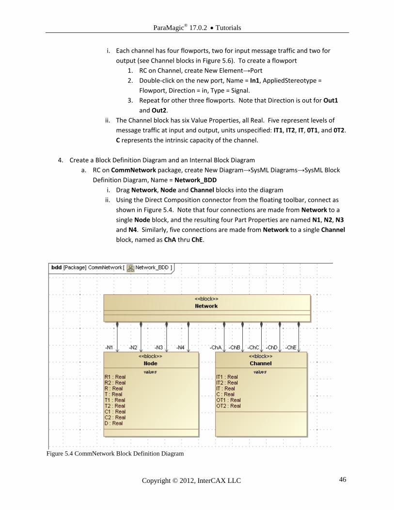
5.2 Step-by-Step Tutorial .................................................................................................................... 44 Step I Create Project ........................................................................................................................... 44 Step II Create Infrastructure ............................................................................................................... 44 Step III Create Structural Model ......................................................................................................... 45 Step IV Create Constraints ................................................................................................................. 48 Step V Create Parametrics Model(s) .................................................................................................. 48 Step VI Validate Parametrics Model .................................................................................................. 50 Step VII Create an Instance ................................................................................................................ 50 Step VIII Solve the Instance ............................................................................................................... 53
6 SysML Parametrics Tutorial - Orbital ............................................................................................ 54
6.1 Objective ............................................................................................................................................ 54 What the User Will Learn .................................................................................................................... 54 System Requirements .......................................................................................................................... 55
6.2 Step-by Step Tutorial ........................................................................................................................ 55 Step I Create Project ........................................................................................................................... 55 Step II Create Infrastructure ............................................................................................................... 55 Step III Create Structural Model ......................................................................................................... 55 Step IV Create Constraints ................................................................................................................. 57 Step V Create Parametrics Model ....................................................................................................... 59 Step VI Validate Parametrics Model .................................................................................................. 60 Step VII Create an Instance ................................................................................................................ 60 Step VIII Solve the Instance ............................................................................................................... 65
7 SysML Parametrics Tutorial - HomeHeating ................................................................................ 68
7.1 Objective ............................................................................................................................................ 68 What the User Will Learn .................................................................................................................... 68
7.2 Step-by Step Tutorial ........................................................................................................................ 69 Step I Create Project ........................................................................................................................... 69 Step II Create Infrastructure ............................................................................................................... 69 Step III Create Structural Model ......................................................................................................... 69 Step IV Create Constraints ................................................................................................................. 70 Step V Create Parametrics Model ....................................................................................................... 72 Step VI Validate Parametrics Model .................................................................................................. 72 Step VII Create an Instance ................................................................................................................ 72 Step VIII Solve the Instance ............................................................................................................... 75
ParaMagic® 17.0.2 Tutorials
Copyright © 2012, InterCAX LLC 3
8 SysML Parametrics Tutorial – LittleEye Trade Study .................................................................. 77
8.1 Objective ............................................................................................................................................ 77 What the User Will Learn .................................................................................................................... 77
8.2 Step-by-Step Tutorial .................................................................................................................... 77 Step VII Set-up a Trade Study ............................................................................................................. 77 Step VIII Run the Trade Study ........................................................................................................... 79
9 SysML Parametrics Tutorial - Electronics ...................................................................................... 80
9.1 Objective ............................................................................................................................................ 80
9.2 Step-by-Step Tutorial .................................................................................................................... 81 Step I Create Project ........................................................................................................................... 81 Step II Create Infrastructure ............................................................................................................... 81 Step III Create Structural Model ......................................................................................................... 81 Step IV Create Constraints ................................................................................................................. 83 Step V Create Parametrics Model ....................................................................................................... 84 Step VI Validate Parametrics Model .................................................................................................. 85 Step VII Create an Instance ................................................................................................................ 85 Step VIII Solve the Instance ............................................................................................................... 87 Step VII Create an Instance (Second Configuration) ......................................................................... 88 Step VIII Solve the Instance (Second Configuration) ........................................................................ 88

ParaMagic® 17.0.2 Tutorials
Copyright © 2012, InterCAX LLC 4
1 INTRODUCTION AND REVIEW
1.1 Introduction
The primary purposes of SysML up to this point have been Documentation, precise specification
of system design, and Communication, sharing the design among multiple parties. Adding parametric
execution to SysML enables additional purposes,
Consistency, enforcing internal relationships to insure a coherent, self-consistent data set;
Simulation, evaluating the performance, cost and other parameters of the system design;
Verification, integrating checks of system properties against requirements.
Our general approach for tutorials on creating SysML model with parametrics follows
I. Create Project
II. Create Infrastructure
III. Create Structural Model
IV. Create Constraints
V. Create Parametric Model
VI. Validate Parametric Model
VII. Create an Instance
VIII. Solve the Instance
Steps I and III are equivalent to those already performed by SysML users and it is generally
straightforward to add parametrics to existing models. Step II, Infrastructure, requires the user to import a
standard module into each project to enable parametrics execution. Step IV, Constraints, has the user
define the generic mathematical relationships to be used. Step V “wires up” the connections between
numerical attributes in the structural model and the constraint equations, using one or more SysML
Parametric diagrams. Step VI, Validation, checks that the parametrics model is properly constructed for
the InterCAX plug-in. In Step VII, the user must create a specific example of the model, populating some
of the attributes in the model with real numbers and identifying others as unknowns to be calculated in
Step VIII. This outline is not offered as a general methodology for building parametric models, so much
as a helpful outline for organizing the detailed instructions.
Before the user can reproduce these tutorials, the user must install and configure
MagicDraw 17.0.1
MagicDraw SysML 17.0.1 plug-in
ParaMagic 17.0.1 or 17.0.1 Lite, the InterCAX SysML Parametrics plug-in for
MagicDraw
Mathematica 8 (Wolfram Research) and/or OpenModelica 1.7 (or 1.8)
Several features of the tutorial models are specific to the MagicDraw and ParaMagic 17.0.1 and may not
work correctly with earlier versions. Contact NoMagic or InterCAX for further information.
The fifth and sixth tutorials use two additional tools:
Microsoft Excel
MATLAB (The MathWorks, Inc.) with the Simulink toolkit
In each case, refer to the installation instructions in the appropriate user guide. It is also necessary to
modify ParaMagic so that it points to the copy of Mathematica. We assume that MagicDraw, ParaMagic,

ParaMagic® 17.0.2 Tutorials
Copyright © 2012, InterCAX LLC 5
OpenModelica MATLAB and Excel (if required) are all installed on the user’s local machine.
Mathematica may be local or accessed through a web services interface.
The first tutorial, Addition, starts with three objects in the simplest possible relationship, a + b =
c, and describes the steps in minute detail for those unfamiliar not only with parametrics, but with the
MagicDraw SysML plug-in (MagicDraw Version 17.0.1) as well. In the later tutorials, we will hide more
of the procedural detail as we model more complex and realistic systems.
The second tutorial, Satellite, models the weight and power budgets of a satellite system,
introducing concepts of hierarchy, requirements and multiple constraints. The third tutorial, LittleEye,
models the operational capability of an unmanned aerial vehicle, introducing object-oriented
programming in model design and non-arithmetic functions. The fourth tutorial, CommNetwork,
introduces the use of simple elements to build up and simulate more complex networks.
The fifth and sixth tutorials provide an introduction to special features for interfacing to Excel
and MATLAB. The Orbital tutorial shows how Excel may be used to load initial values into a model for
space mission planning and to record parametric simulation results. The HomeHeating tutorial
demonstrates how external functions and scripts programmed in MATLAB can be integrated into the
parametric simulation. MATLAB scripts can, in turn, call Simulink models.
The seventh tutorial extends the LittleEye model from the third tutorial to demonstrate trade
studies. The eighth tutorial, Electronics, introduces complex aggregates and generalization, powerful
features of SysML that allow a simple parametric model to apply to a wide range of concrete system
realizations.
Several of the tutorial models cannot be executed by ParaMagic 17.0.1 Lite because they include
model elements that are not supported, including MATLAB, custom Mathematica and complex aggregate
functions. Table 1.1 summarizes this information.
Tutorial ParaMagic™ ParaMagic™ Lite Addition Yes Yes
Satellite Yes Yes
LittleEye Yes Yes
CommNetwork Yes Yes
Orbital Yes Partial (No Mathematica graphing)
HomeHeating Yes No (MATLAB function and script)
LittleEye Trade Study Yes Yes
Electronics Yes No (complex aggregates)
Table 1.1 Tutorial Applicability for ParaMagic™ and ParaMagic™ Lite
As in many subjects, the best way to learn SysML Parametrics is by doing. The author
recommends building the models described in the first four tutorials, comparing your results with the
figures in the text and exploring variations. There are generally multiple ways to implement any model
and, in a few cases, alternate procedures are described. The author would appreciate user feedback on
errors and unclear descriptions in this document ([email protected]).
1.2 Short Review of SysML
SysML is a powerful and wide-reaching language for modeling systems. In this section, we will review a
few aspects of SysML of special importance to parametrics, to help make sense of the detailed
instructions in the tutorials for new users with limited SysML experience. This is not intended as a broad
introduction or primer on SysML.
SysML supports three major classes of diagrams, which are ways at the looking at the system model:

ParaMagic® 17.0.2 Tutorials
Copyright © 2012, InterCAX LLC 6
Structure diagrams, which describe what the system is composed of. Parametrics is part of
structure and these diagrams are our principal focus in the tutorials.
Behavior diagrams, which describe what the system does. We will not deal with any behavior
diagrams in these tutorials.
Requirements diagrams, which describe the design and performance objectives the system must
meet. We introduce requirements diagrams in the tutorials Satellite and Electronics, to show how
parametrics can help build requirements checking into a system model.
With respect to structure diagrams, there are three important types. These are illustrated in Figure 1.1.
Block definition diagrams (BDD), which describe the organization of the structure, the hierarchy
of system, subsystems, and all the elements that make up the system. In Figure 1.1, the Body,
Engine, and Wheels are elements that belong to the object Automobile, the ownership
relationships shown in black. Our tutorials usually begin by creating a BDD.
Internal block diagrams (IBD), which describe qualitative flows between elements. In Figure 1.1,
gasoline flows from a tank in the Body to the Engine, as shown in red. In the tutorial
CommNetwork, we use an IBD to keep track of message traffic channels between stations, but
IBDs do not affect parametrics directly.
Parametric diagrams (PAR), which describe quantitative relationships between properties of the
elements. In Figure 1.1, mileage, which is a property of Automobile, is a function of the drag of
the Body, the efficiency of the Engine, and so forth in green. Creating and executing parametric
diagrams is the primary focus of these tutorials.
Figure 1.1 Structure diagram relationships
Finally, we need to clarify three types of objects within the system: blocks, part properties, and instances.
Examples are illustrated in Figure 1.2.
Blocks represent a generic object, like the Wheel in Figure 1.2a. A block may have value
properties which describe it, like model number or radius, but these properties typically do not
contain specific values.
Part properties represent usages of a block; i.e. a block as part of some larger system. In Figure
1.2b, Front Wheel and Back Wheel are two separate roles that Wheel plays as part of Motorcycle.
ParaMagic® 17.0.2 Tutorials
Copyright © 2012, InterCAX LLC 7
Instances represent a specific example of a generic object, like WhiteWallRadial in Figure 1.2c.
The value properties have specific values, which may be fixed or calculated from other system
values. ParaMagic executes parametric calculations for specific instances of system models.
Figure 1.2a Block Figure 1.2b Part Properties Figure 1.2c Instance of a Block
1.3 Short Review of Solving Equations
ParaMagic’s primary function is to solve the often-complex network of parametric equations within the
system model, so it is valuable to review a few concepts that will come up in the tutorials.
Causality is the organization of known and unknown variables in the equations. ParaMagic requires the
assignment of a causality state to each variable, which can be done manually by the user or semi-
automatically by the ParaMagic program. The allowable causality states are
Given – a parameter with a known value provided by the user before the ParaMagic calculation.
Target – a parameter with an initially unknown value that the user specifically wishes to
calculate. Each ParaMagic calculation requires at least one target variable.
Undefined – a parameter with an initially unknown value, that may be calculated in the process of
solving for the target.
Ancillary – an undefined parameter after its value has been calculated by ParaMagic. It can’t be
assigned before solution.
In the text, causalities are denoted in italics.
As an example, consider the two equation network
a + b = c c + d = e
Our objective is to calculate e, which is assigned target causality. If we know beforehand that a = 3, b =
2, and d = 5, these parameters would be assigned given causality. The remaining parameter, c, could be
assigned undefined causality. When c is solved for in calculating e, its causality changes to ancillary. It is
also possible to assign both c and e to target causality, but multiplying targets unnecessarily may slow
down solving for larger equation sets.
Assigning causality requires consideration of overconstraint/underconstraint. Underconstraint occurs
when insufficient variables are assigned values (and given causality) to calculate the targets. For
example, in the equations above, if we set a = 3 and d = 5, there are an infinite number of solutions for e

ParaMagic® 17.0.2 Tutorials
Copyright © 2012, InterCAX LLC 8
and the equation set is underconstrained. Alternately, if we assigned a = 3, b = 2, d = 5, and e = 6, the
system is overconstrained and there are zero possible solutions for c. In general, Mathematica and
OpenModelica, the solver engines for ParaMagic, will alert the user when overconstraint/underconstraint
occurs, but some analysis by the user might be required to determine the correct number of knowns for
complex equation sets. In general, Mathematica is more robust in dealing with overconstraint/
underconstraint issues than OpenModelica.
A third issue to consider in assigning causality is reversibility. Some equations, like c = a + b, are
reversible or acausal. We can solve for c knowing a and b, or we can solve for a, knowing b and c.
Other equations are not. a = sin(b) can be solved uniquely for a knowing b, but may have multiple
possible solutions for b knowing a (e.g. for a = 0, b can be equal to 0, π, 2π, …). Similarly, a =
minimum(b,c,d) is not always reversible. ParaMagic treats these types of equations as “one-way” and
causality assignments must take this into account.
ParaMagic® 17.0.2 Tutorials
Copyright © 2012, InterCAX LLC 9
2 SYSML PARAMETRICS TUTORIAL - ADDITION
2.1 Objective
Create a SysML project with three elements. Each element has one attribute. The attribute of the
third element is the sum of the first two attributes. Create an instance of this model and solve for the third
attribute parametrically.
Figure 2.1 Outline of Objective
What the User Will Learn
Creating the basic elements of SysML models in MagicDraw: blocks, properties, constraints,
etc.
Building a SysML parametrics model and diagram
Creating a instance of the model with input and output parameters
Opening and using the ParaMagic browser window
Exporting a parametrics model to Mathematica
2.2 Step-by-Step Tutorial
Step I Create Project
1. Open MagicDraw.
2. On MagicDraw menu bar, select Options→Perspectives→Perspectives and set to System
Engineer.
3. Create new project
a. On MagicDraw menu bar, select File→New Project,
b. In New Project window (Figure 2.2), choose SysML Project,
c. Set Name = Addition. User-assigned names and constraints for specific SysML
elements are given in Bold.
d. Set or browse for location to save project.
4. Create a package within the project
a. RC (Right-click) on Data folder in Containment tree (Figure 2.3)
b. Select New Element→Package
c. Enter Name = Addition
ParaMagic® 17.0.2 Tutorials
Copyright © 2012, InterCAX LLC 10
Note for Mac Users: Right-Click is substituted by the Mac keystroke: Control-Click. While ParaMagic is
compatible for both Windows and Macintosh operating systems, certain keystrokes and paths are
bound to vary. The author will make note of any significant differences in ParaMagic for Mac users
hereafter.
Figure 2.2 New Project window Figure 2.3 Creating Package in Data folder
Step II Create Infrastructure
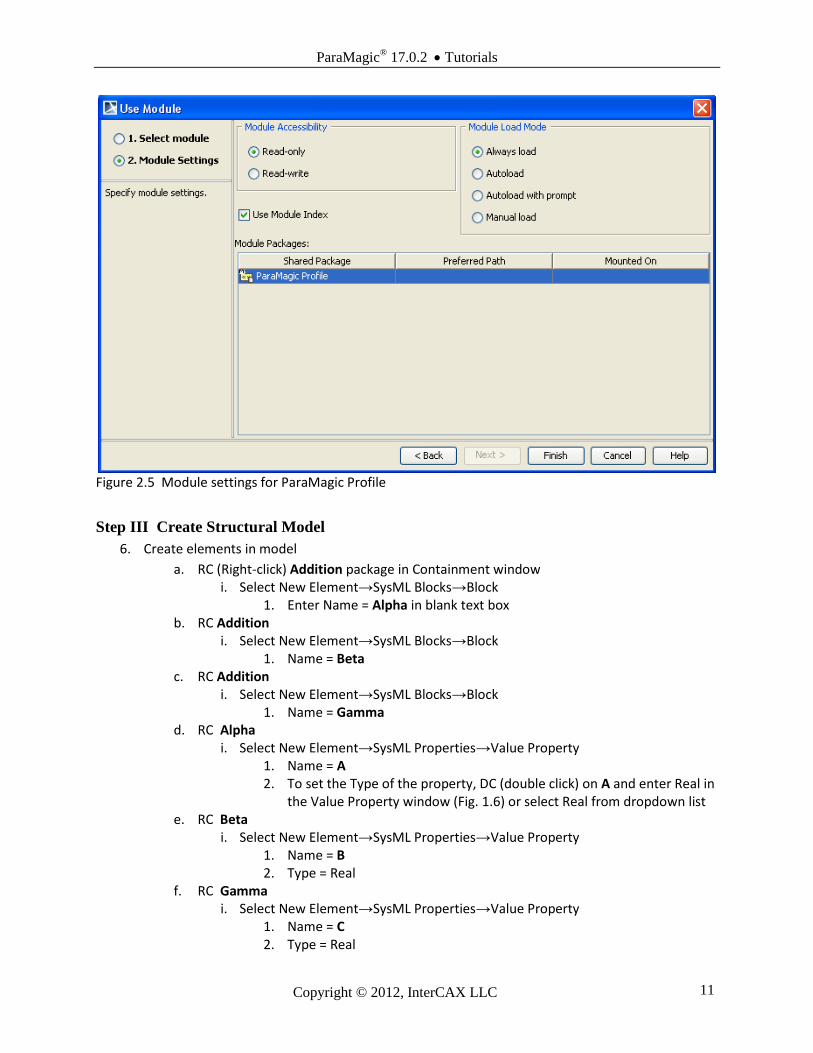
5. Install ParaMagic Profile module
a. On MagicDraw menu bar, select File→Use Module… and select as below (Figure 2.4).
This loads a module containing all the ParaMagic features as part of the project.
i. Click Next and Finish (Figure 2.5).
Figure 2.4 Use Module window
ParaMagic® 17.0.2 Tutorials
Copyright © 2012, InterCAX LLC 11
Figure 2.5 Module settings for ParaMagic Profile
Step III Create Structural Model
6. Create elements in model
a. RC (Right-click) Addition package in Containment window i. Select New Element→SysML Blocks→Block
1. Enter Name = Alpha in blank text box b. RC Addition
i. Select New Element→SysML Blocks→Block 1. Name = Beta
c. RC Addition i. Select New Element→SysML Blocks→Block
1. Name = Gamma d. RC Alpha
i. Select New Element→SysML Properties→Value Property 1. Name = A 2. To set the Type of the property, DC (double click) on A and enter Real in
the Value Property window (Fig. 1.6) or select Real from dropdown list e. RC Beta
i. Select New Element→SysML Properties→Value Property 1. Name = B 2. Type = Real
f. RC Gamma i. Select New Element→SysML Properties→Value Property
1. Name = C 2. Type = Real

ParaMagic® 17.0.2 Tutorials
Copyright © 2012, InterCAX LLC 12
Figure 2.6 Value Property window, enter Type
7. Create a block definition diagram, a graphical view of the entire system
a. RC Addition
b. Select New Diagram→SysML Diagrams→SysML Block Definition Diagram
i. Name = AdditionBDD
c. Drag Alpha, Beta, and Gamma from Containment window into AdditionBDD (Figure 2.7)
i. To rearrange position, drag using top half of block.
ii. To resize block, click on top half of block and use cursors at corners
iii. If attributes (e.g. B) are not listed inside the blocks, display the attributes by,
1. RC on block,
2. choose Presentation Options,
3. uncheck Suppress Attributes.
Alternatives: To show or hide the interior features of a block, right-click on the block and use the Symbol Properties, Edit Compartment and Presentation Options commands. Alternately, click on the block and look for small plus and minus icons on the left edge to display or suppress interior features.
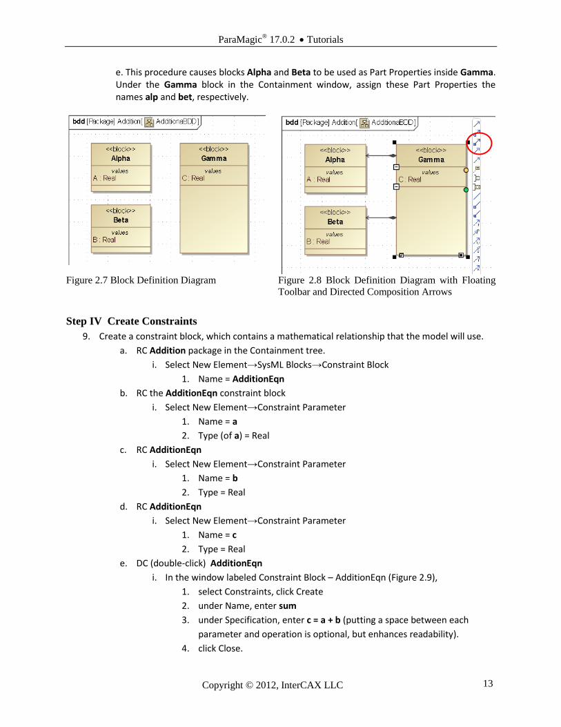
8. Create relationships between elements of the model. Alpha and Beta can be used as parts of
Gamma.
a. Click on Gamma in the Block Definition Diagram
b. Select Directed Composition arrow from floating toolbar (arrow with solid diamond at
base).
c. Drag end of arrow to Alpha
d. Repeat steps a-c for Beta (Figure 2.8)
ParaMagic® 17.0.2 Tutorials
Copyright © 2012, InterCAX LLC 13
e. This procedure causes blocks Alpha and Beta to be used as Part Properties inside Gamma. Under the Gamma block in the Containment window, assign these Part Properties the names alp and bet, respectively.
Figure 2.7 Block Definition Diagram Figure 2.8 Block Definition Diagram with Floating
Toolbar and Directed Composition Arrows
Step IV Create Constraints
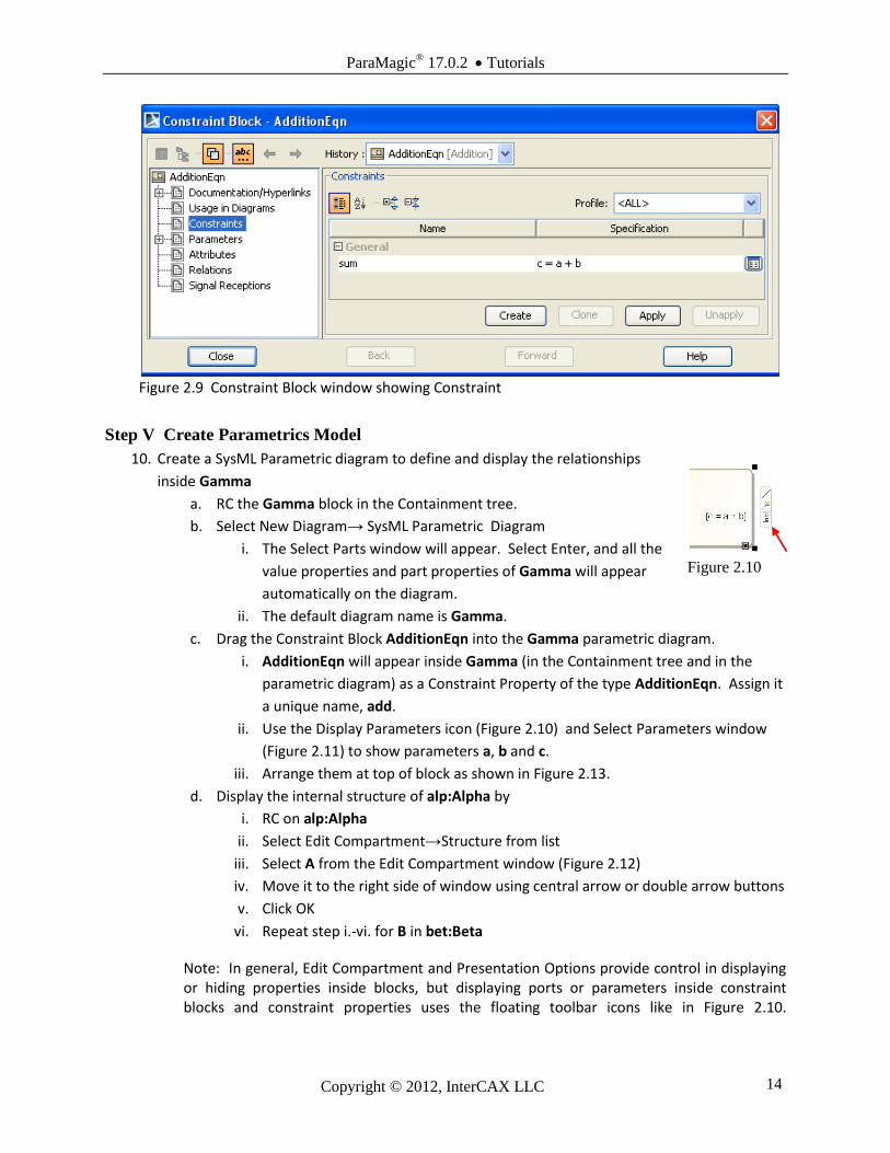
9. Create a constraint block, which contains a mathematical relationship that the model will use.
a. RC Addition package in the Containment tree.
i. Select New Element→SysML Blocks→Constraint Block
1. Name = AdditionEqn
b. RC the AdditionEqn constraint block
i. Select New Element→Constraint Parameter
1. Name = a
2. Type (of a) = Real
c. RC AdditionEqn
i. Select New Element→Constraint Parameter
1. Name = b
2. Type = Real
d. RC AdditionEqn
i. Select New Element→Constraint Parameter
1. Name = c
2. Type = Real
e. DC (double-click) AdditionEqn
i. In the window labeled Constraint Block – AdditionEqn (Figure 2.9),
1. select Constraints, click Create
2. under Name, enter sum
3. under Specification, enter c = a + b (putting a space between each
parameter and operation is optional, but enhances readability).
4. click Close.
ParaMagic® 17.0.2 Tutorials
Copyright © 2012, InterCAX LLC 14
Figure 2.9 Constraint Block window showing Constraint
Step V Create Parametrics Model
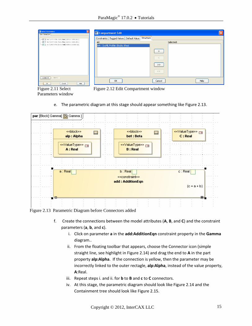
10. Create a SysML Parametric diagram to define and display the relationships
inside Gamma
a. RC the Gamma block in the Containment tree.
b. Select New Diagram→ SysML Parametric Diagram
i. The Select Parts window will appear. Select Enter, and all the
value properties and part properties of Gamma will appear
automatically on the diagram.
ii. The default diagram name is Gamma.
c. Drag the Constraint Block AdditionEqn into the Gamma parametric diagram.
i. AdditionEqn will appear inside Gamma (in the Containment tree and in the
parametric diagram) as a Constraint Property of the type AdditionEqn. Assign it
a unique name, add.
ii. Use the Display Parameters icon (Figure 2.10) and Select Parameters window
(Figure 2.11) to show parameters a, b and c.
iii. Arrange them at top of block as shown in Figure 2.13.
d. Display the internal structure of alp:Alpha by
i. RC on alp:Alpha
ii. Select Edit Compartment→Structure from list
iii. Select A from the Edit Compartment window (Figure 2.12)
iv. Move it to the right side of window using central arrow or double arrow buttons
v. Click OK
vi. Repeat step i.-vi. for B in bet:Beta
Note: In general, Edit Compartment and Presentation Options provide control in displaying or hiding properties inside blocks, but displaying ports or parameters inside constraint blocks and constraint properties uses the floating toolbar icons like in Figure 2.10.
Figure 2.10
ParaMagic® 17.0.2 Tutorials
Copyright © 2012, InterCAX LLC 15
Figure 2.11 Select
Parameters window
Figure 2.12 Edit Compartment window
e. The parametric diagram at this stage should appear something like Figure 2.13.
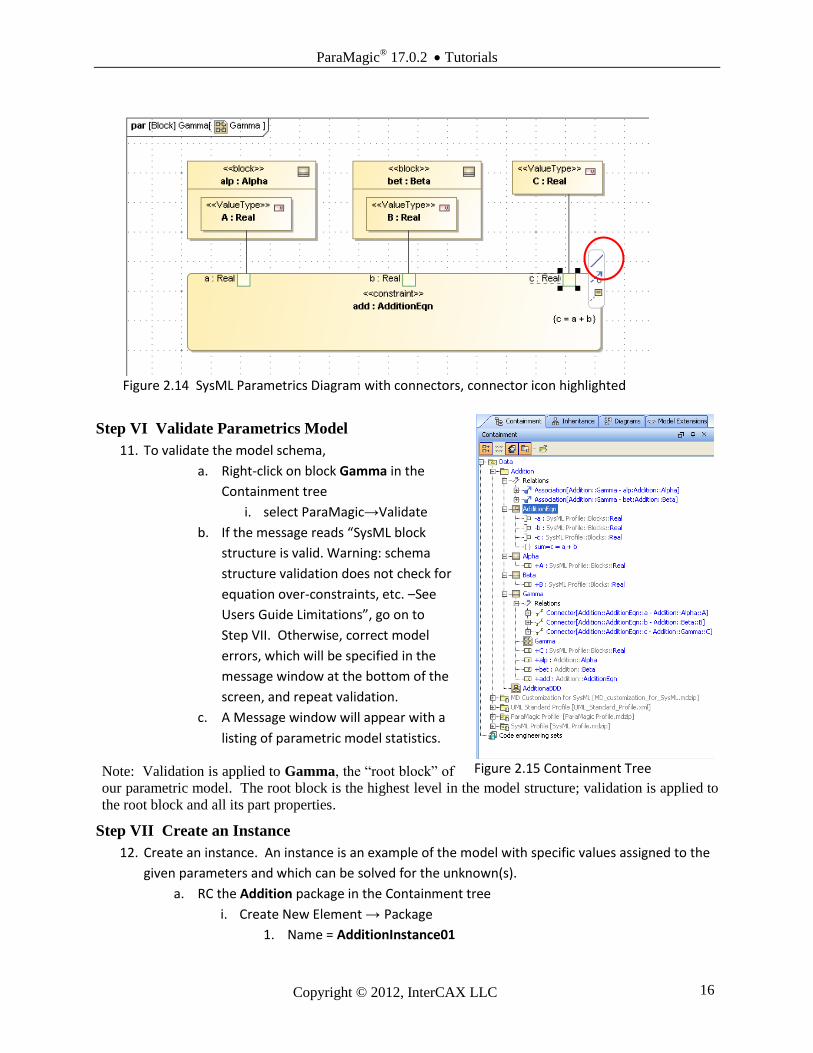
Figure 2.13 Parametric Diagram before Connectors added
f. Create the connections between the model attributes (A, B, and C) and the constraint
parameters (a, b, and c).
i. Click on parameter a in the add:AdditionEqn constraint property in the Gamma
diagram..
ii. From the floating toolbar that appears, choose the Connector icon (simple
straight line, see highlight in Figure 2.14) and drag the end to A in the part
property alp:Alpha. If the connection is yellow, then the parameter may be
incorrectly linked to the outer rectagle, alp:Alpha, instead of the value property,
A:Real.
iii. Repeat steps i. and ii. for b to B and c to C connectors.
iv. At this stage, the parametric diagram should look like Figure 2.14 and the
Containment tree should look like Figure 2.15.
ParaMagic® 17.0.2 Tutorials
Copyright © 2012, InterCAX LLC 16
Figure 2.14 SysML Parametrics Diagram with connectors, connector icon highlighted
Step VI Validate Parametrics Model
11. To validate the model schema,
a. Right-click on block Gamma in the
Containment tree
i. select ParaMagic→Validate
b. If the message reads “SysML block
structure is valid. Warning: schema
structure validation does not check for
equation over-constraints, etc. –See
Users Guide Limitations”, go on to
Step VII. Otherwise, correct model
errors, which will be specified in the
message window at the bottom of the
screen, and repeat validation.
c. A Message window will appear with a
listing of parametric model statistics.
Note: Validation is applied to Gamma, the “root block” of
our parametric model. The root block is the highest level in the model structure; validation is applied to
the root block and all its part properties.
Step VII Create an Instance
12. Create an instance. An instance is an example of the model with specific values assigned to the
given parameters and which can be solved for the unknown(s).
a. RC the Addition package in the Containment tree
i. Create New Element → Package
1. Name = AdditionInstance01
Figure 2.15 Containment Tree
ParaMagic® 17.0.2 Tutorials
Copyright © 2012, InterCAX LLC 17
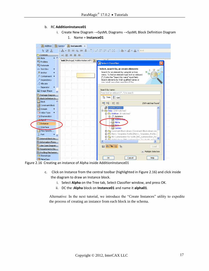
b. RC AdditionInstance01
i. Create New Diagram →SysML Diagrams →SysML Block Definition Diagram
1. Name = Instance01
Figure 2.16 Creating an instance of Alpha inside AdditionInstance01
c. Click on Instance from the central toolbar (highlighted in Figure 2.16) and click inside
the diagram to draw an Instance block.
i. Select Alpha on the Tree tab, Select Classifier window, and press OK.
ii. DC the :Alpha block on Instance01 and name it alpha01.
Alternative: In the next tutorial, we introduce the “Create Instances” utility to expedite
the process of creating an instance from each block in the schema.
ParaMagic® 17.0.2 Tutorials
Copyright © 2012, InterCAX LLC 18
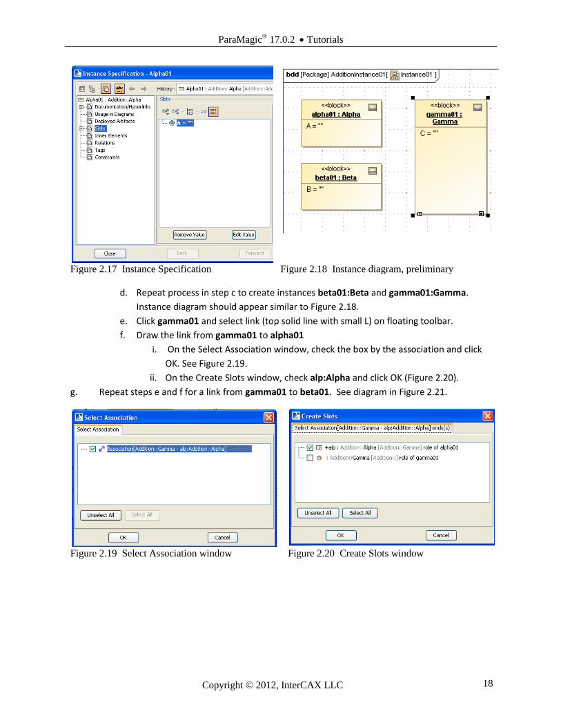
Figure 2.17 Instance Specification Figure 2.18 Instance diagram, preliminary
d. Repeat process in step c to create instances beta01:Beta and gamma01:Gamma.
Instance diagram should appear similar to Figure 2.18.
e. Click gamma01 and select link (top solid line with small L) on floating toolbar.
f. Draw the link from gamma01 to alpha01
i. On the Select Association window, check the box by the association and click
OK. See Figure 2.19.
ii. On the Create Slots window, check alp:Alpha and click OK (Figure 2.20).
g. Repeat steps e and f for a link from gamma01 to beta01. See diagram in Figure 2.21.
Figure 2.19 Select Association window Figure 2.20 Create Slots window
ParaMagic® 17.0.2 Tutorials
Copyright © 2012, InterCAX LLC 19
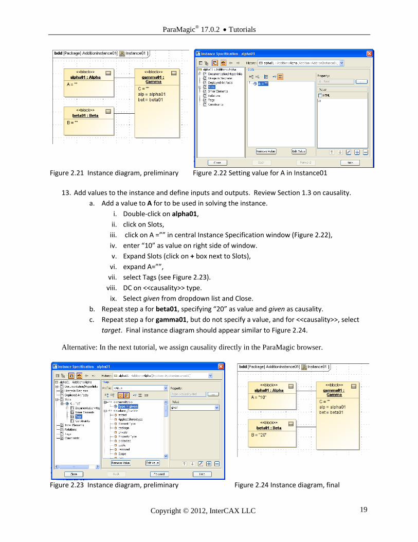
Figure 2.21 Instance diagram, preliminary Figure 2.22 Setting value for A in Instance01
13. Add values to the instance and define inputs and outputs. Review Section 1.3 on causality.
a. Add a value to A for to be used in solving the instance.
i. Double-click on alpha01,
ii. click on Slots,
iii. click on A =”” in central Instance Specification window (Figure 2.22),
iv. enter “10” as value on right side of window.
v. Expand Slots (click on + box next to Slots),
vi. expand A=””,
vii. select Tags (see Figure 2.23).
viii. DC on <<causality>> type.
ix. Select given from dropdown list and Close.
b. Repeat step a for beta01, specifying “20” as value and given as causality.
c. Repeat step a for gamma01, but do not specify a value, and for <<causality>>, select
target. Final instance diagram should appear similar to Figure 2.24.
Alternative: In the next tutorial, we assign causality directly in the ParaMagic browser.
Figure 2.23 Instance diagram, preliminary Figure 2.24 Instance diagram, final

ParaMagic® 17.0.2 Tutorials
Copyright © 2012, InterCAX LLC 20
Step VIII Solve the Instance
14. Run the parametric solver
a. RC gamma01 (instance of the root block) in the Containment tree.
b. Select ParaMagic→Browse. Expand the alp and bet part properties in the browser
(click the + sign beside them) and it should appear as in Figure 2.25.
Figure 2.25 ParaMagic Browser window
c. Press “Solve”
i. The ????? symbols in the target variables should change to their calculated
values, in this case C = 30 (Figure 2.26).
d. Press “Update to SysML”. C=30 should appear in the Containment tree and Instance
diagram.
Figure 2.26 Browser window with solution
ParaMagic® 17.0.2 Tutorials
Copyright © 2012, InterCAX LLC 21
3 SYSML PARAMETRICS TUTORIAL - SATELLITE
3.1 Objective
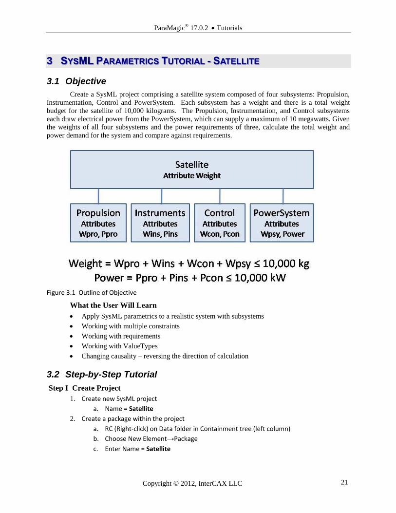
Create a SysML project comprising a satellite system composed of four subsystems: Propulsion,
Instrumentation, Control and PowerSystem. Each subsystem has a weight and there is a total weight
budget for the satellite of 10,000 kilograms. The Propulsion, Instrumentation, and Control subsystems
each draw electrical power from the PowerSystem, which can supply a maximum of 10 megawatts. Given
the weights of all four subsystems and the power requirements of three, calculate the total weight and
power demand for the system and compare against requirements.
Figure 3.1 Outline of Objective
What the User Will Learn
Apply SysML parametrics to a realistic system with subsystems
Working with multiple constraints
Working with requirements
Working with ValueTypes
Changing causality – reversing the direction of calculation
3.2 Step-by-Step Tutorial
Step I Create Project
1. Create new SysML project
a. Name = Satellite
2. Create a package within the project
a. RC (Right-click) on Data folder in Containment tree (left column)
b. Choose New Element→Package
c. Enter Name = Satellite

ParaMagic® 17.0.2 Tutorials
Copyright © 2012, InterCAX LLC 22
Step II Create Infrastructure
3. Install ParaMagic Profile module, same as in the first tutorial.
Step III Create Structural Model
4. Create elements in model
a. RC on Satellite
i. Create New Element→Package
1. Name = ValueTypes
ii. RC on ValueTypes, create New Element→SysML Values→ ValueType
1. Name = Kilowatt
2. Base Classifier = Real
a. DC on Kilowatt in Containment tree
b. In Value Type – Kilowatt window click to the right of Base
Classifier row in table
c. Click on button with three dots
d. In Select Elements window, enter Real in Search by name
text box
e. Select Real (SysML Profile::Blocks)
f. Click OK and Close.
iii. RC on ValueTypes, create New Element→SysML Values→ ValueType
1. Name = Kilogram
2. Base Classifier = Real
b. RC Satellite
i. Create New Element→SysML Blocks→Block
1. Name = SatelliteSystem
ii. In SatelliteSystem, create three new value properties
1. Name = Weight, Type = Kilogram
2. Name = Weight_MOS, Type = Real
3. Name = Power_MOS,
4. Type = Real
Discussion – ValueTypes, Units, and Dimensions
We frequently want to apply units to a value property, for example, electrical power in our model
will be expressed in kilowatts. We do this by assigning a ValueType to the value property. We can
use the Type property to make this assignment. We create two new ValueTypes in step 4.a above,
Kilograms and Kilowatts. ParaMagic expects valuetypes used for parameters to be subtypes of the
Real valuetype, so we use the Base Classifier entry to make this assignment (alternatively, the
quantityKind field can be populated, see ParaMagic User Guide).
Assigning valuetypes to properties makes the model more exact and helps identify mismatches
when block properties and constraint parameters are linked in parametric diagrams. Note that units
are not assigned to value properties directly, so the Kilogram unit in the MD SysML profile is not
used in step 4.b.ii.1 above. The full description of the relationship between ValueTypes, Units and
Dimensions is described in the MagicDraw User Guide.
ParaMagic® 17.0.2 Tutorials
Copyright © 2012, InterCAX LLC 23
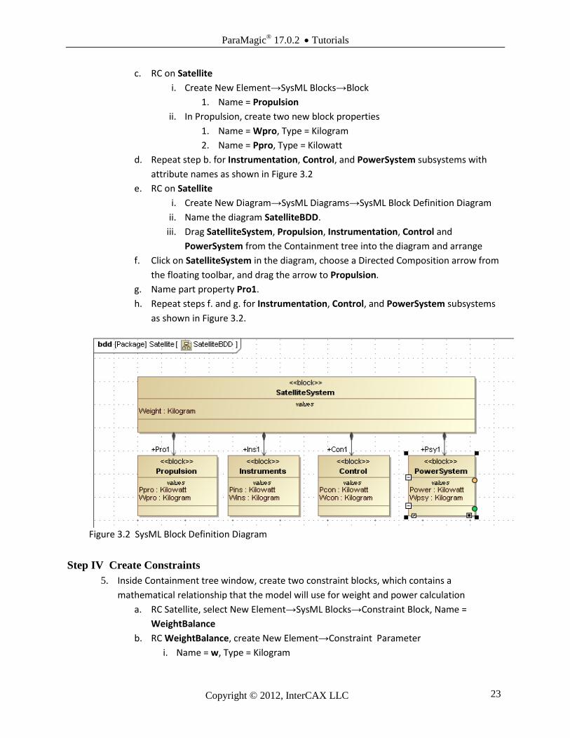
c. RC on Satellite
i. Create New Element→SysML Blocks→Block
1. Name = Propulsion
ii. In Propulsion, create two new block properties
1. Name = Wpro, Type = Kilogram
2. Name = Ppro, Type = Kilowatt
d. Repeat step b. for Instrumentation, Control, and PowerSystem subsystems with
attribute names as shown in Figure 3.2
e. RC on Satellite
i. Create New Diagram→SysML Diagrams→SysML Block Definition Diagram
ii. Name the diagram SatelliteBDD.
iii. Drag SatelliteSystem, Propulsion, Instrumentation, Control and
PowerSystem from the Containment tree into the diagram and arrange
f. Click on SatelliteSystem in the diagram, choose a Directed Composition arrow from
the floating toolbar, and drag the arrow to Propulsion.
g. Name part property Pro1.
h. Repeat steps f. and g. for Instrumentation, Control, and PowerSystem subsystems
as shown in Figure 3.2.
Figure 3.2 SysML Block Definition Diagram
Step IV Create Constraints
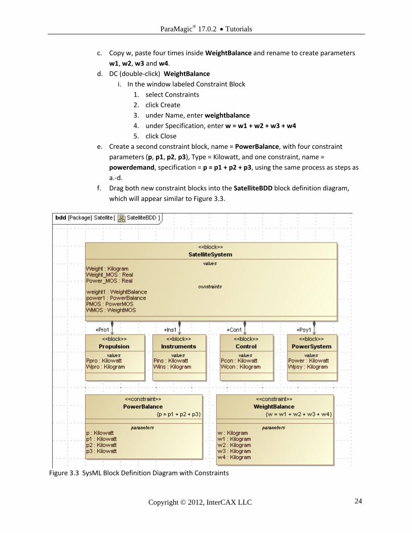
5. Inside Containment tree window, create two constraint blocks, which contains a
mathematical relationship that the model will use for weight and power calculation
a. RC Satellite, select New Element→SysML Blocks→Constraint Block, Name =
WeightBalance
b. RC WeightBalance, create New Element→Constraint Parameter
i. Name = w, Type = Kilogram
ParaMagic® 17.0.2 Tutorials
Copyright © 2012, InterCAX LLC 24
c. Copy w, paste four times inside WeightBalance and rename to create parameters
w1, w2, w3 and w4.
d. DC (double-click) WeightBalance
i. In the window labeled Constraint Block
1. select Constraints
2. click Create
3. under Name, enter weightbalance
4. under Specification, enter w = w1 + w2 + w3 + w4
5. click Close
e. Create a second constraint block, name = PowerBalance, with four constraint
parameters (p, p1, p2, p3), Type = Kilowatt, and one constraint, name =
powerdemand, specification = p = p1 + p2 + p3, using the same process as steps as
a.-d.
f. Drag both new constraint blocks into the SatelliteBDD block definition diagram,
which will appear similar to Figure 3.3.
Figure 3.3 SysML Block Definition Diagram with Constraints
ParaMagic® 17.0.2 Tutorials
Copyright © 2012, InterCAX LLC 25
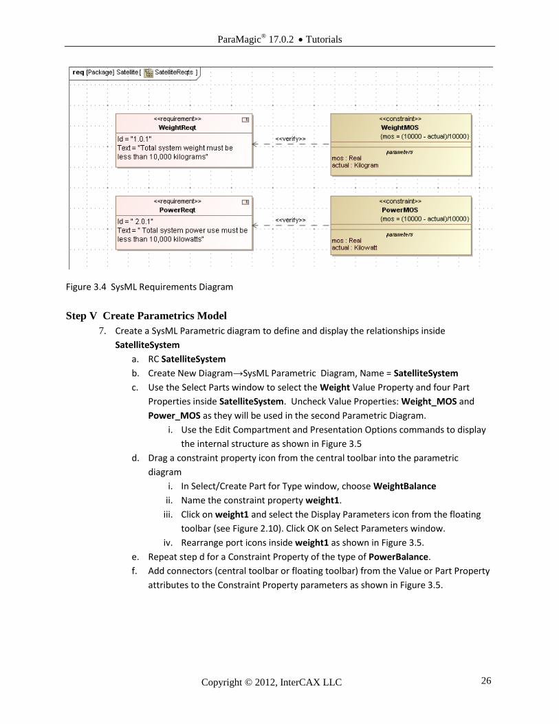
6. Create a Requirements diagram to show the specifications for the Satellite system. The
purpose of a Requirements diagram is to make clear the requirements the system must
meet and how these requirements tie to specific values of the model. For our purpose, we
can pair each Requirement with a Constraint Block that mirrors it, making it easy to
automatically verify the constraint when ParaMagic is executed.
a. RC on Satellite, create New Element→Package, Name = SatelliteReqts
b. RC on SatelliteReqts, create New Diagram→SysML Diagrams→SysML Requirements
Diagram, Name = SatelliteReqts
c. Drag two requirements blocks from the center toolbar into the diagram
i. Name = WeightReqt, id = 1.0.1, text = Total system weight must be less than
10,000 kilograms
ii. Name = PowerReqt, id = 2.0.1, text = Total system power use must be
less than 10,000 kilowatts
d. RC on SatelliteReqts, create New Element→SysML Blocks→Constraint Block
i. Name = WeightMOS (Margin of Safety)
e. RC on WeightMOS (in containment tree),
i. Create a New Element→Constraint Parameter, Name = mos, Type = Real
ii. Create a New Element→Constraint Parameter, Name = actual, Type =
Kilogram
iii. Create a constraint, Name = wtmos, Specification = mos = (10000 -
actual)/10000. This constraint calculates the margin of safety as the
difference between the target value, 10,000 kg, and the actual weight as
calculated, divided by the target value. It will be positive if system weight is
below the target value, negative if it exceeds the target.
f. Repeat step e. for PowerMOS (see Figure 3.4 for specifics)
g. Drag PowerMOS and WeightMOS into the Requirements diagram
h. Use the Verify arrow (central toolbar) to show the relationship between each
Constraint Block and the Requirement it verifies.
ParaMagic® 17.0.2 Tutorials
Copyright © 2012, InterCAX LLC 26
Figure 3.4 SysML Requirements Diagram
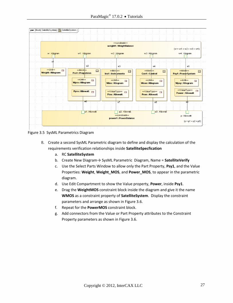
Step V Create Parametrics Model
7. Create a SysML Parametric diagram to define and display the relationships inside
SatelliteSystem
a. RC SatelliteSystem
b. Create New Diagram→SysML Parametric Diagram, Name = SatelliteSystem
c. Use the Select Parts window to select the Weight Value Property and four Part
Properties inside SatelliteSystem. Uncheck Value Properties: Weight_MOS and
Power_MOS as they will be used in the second Parametric Diagram.
i. Use the Edit Compartment and Presentation Options commands to display
the internal structure as shown in Figure 3.5
d. Drag a constraint property icon from the central toolbar into the parametric
diagram
i. In Select/Create Part for Type window, choose WeightBalance
ii. Name the constraint property weight1.
iii. Click on weight1 and select the Display Parameters icon from the floating
toolbar (see Figure 2.10). Click OK on Select Parameters window.
iv. Rearrange port icons inside weight1 as shown in Figure 3.5.
e. Repeat step d for a Constraint Property of the type of PowerBalance.
f. Add connectors (central toolbar or floating toolbar) from the Value or Part Property
attributes to the Constraint Property parameters as shown in Figure 3.5.
ParaMagic® 17.0.2 Tutorials
Copyright © 2012, InterCAX LLC 27
Figure 3.5 SysML Parametrics Diagram
8. Create a second SysML Parametric diagram to define and display the calculation of the
requirements verification relationships inside SatelliteSpecfication
a. RC SatelliteSystem
b. Create New Diagram→ SysML Parametric Diagram, Name = SatelliteVerify
c. Use the Select Parts Window to allow only the Part Property, Psy1, and the Value
Properties: Weight, Weight_MOS, and Power_MOS, to appear in the parametric
diagram.
d. Use Edit Compartment to show the Value property, Power, inside Psy1.
e. Drag the WeightMOS constraint block inside the diagram and give it the name
WMOS as a constraint property of SatelliteSystem. Display the constraint
parameters and arrange as shown in Figure 3.6.
f. Repeat for the PowerMOS constraint block.
g. Add connectors from the Value or Part Property attributes to the Constraint
Property parameters as shown in Figure 3.6.

ParaMagic® 17.0.2 Tutorials
Copyright © 2012, InterCAX LLC 28
Figure 3.6 SysML Parametrics Diagram
Step VI Validate Parametrics Model
9. To validate the model schema, RC on SatelliteSystem, the root block, in the Containment
tree and select ParaMagic→Validate.
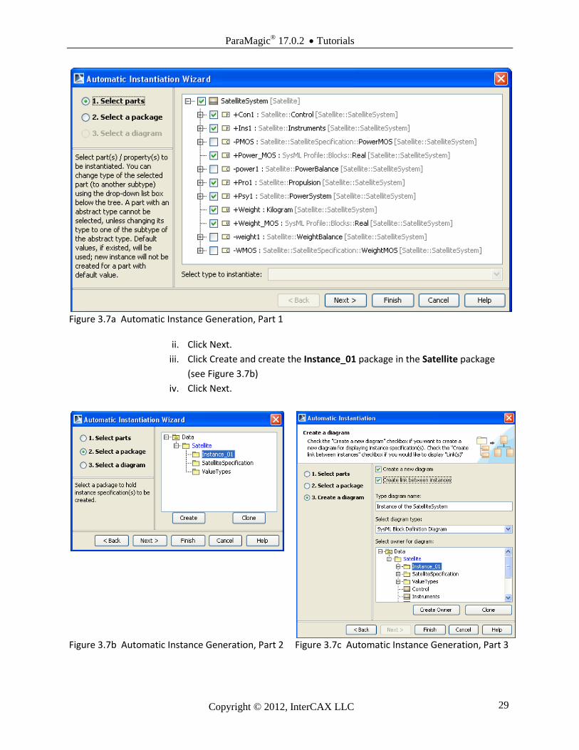
Step VII Create an Instance
10. Create an instance by creating a new block definition diagram containing the model, the
elements whose attributes are givens or unknowns in the calculation. In the first tutorial,
we created the diagrams and instances individually. In this example, we use the
Instantiation Wizard, which can create complex instances more efficiently, particularly
where there are many elements.
a. RC on SatelliteSystem (the root block) and select Create Instance…
i. The Automatic Instantiation Wizard is launched as in Figure 3.7a.
Note: The shortcuts taught in this tutorial, including Create Instances… (step 10) and entering the values
and causalities directly into the ParaMagic browser (step 11) can be quicker than the manual entry
methods shown in the first tutorial. ParaMagic has the ability to create instances and set values directly
from Excel spreadsheets (see the Orbital tutorial for an example), which can be even quicker for more
complex models.
ParaMagic® 17.0.2 Tutorials
Copyright © 2012, InterCAX LLC 29
Figure 3.7a Automatic Instance Generation, Part 1
ii. Click Next.
iii. Click Create and create the Instance_01 package in the Satellite package
(see Figure 3.7b)
iv. Click Next.
Figure 3.7b Automatic Instance Generation, Part 2
Figure 3.7c Automatic Instance Generation, Part 3

ParaMagic® 17.0.2 Tutorials
Copyright © 2012, InterCAX LLC 30
v. Click the “Create a new diagram” checkbox (see Figure 3.7c).
vi. Diagram name = Instance_01, Type = SysML Block Definition Diagram.
vii. Click Finish.
b. The diagram Instance_01 looks similar to Figure 3.8
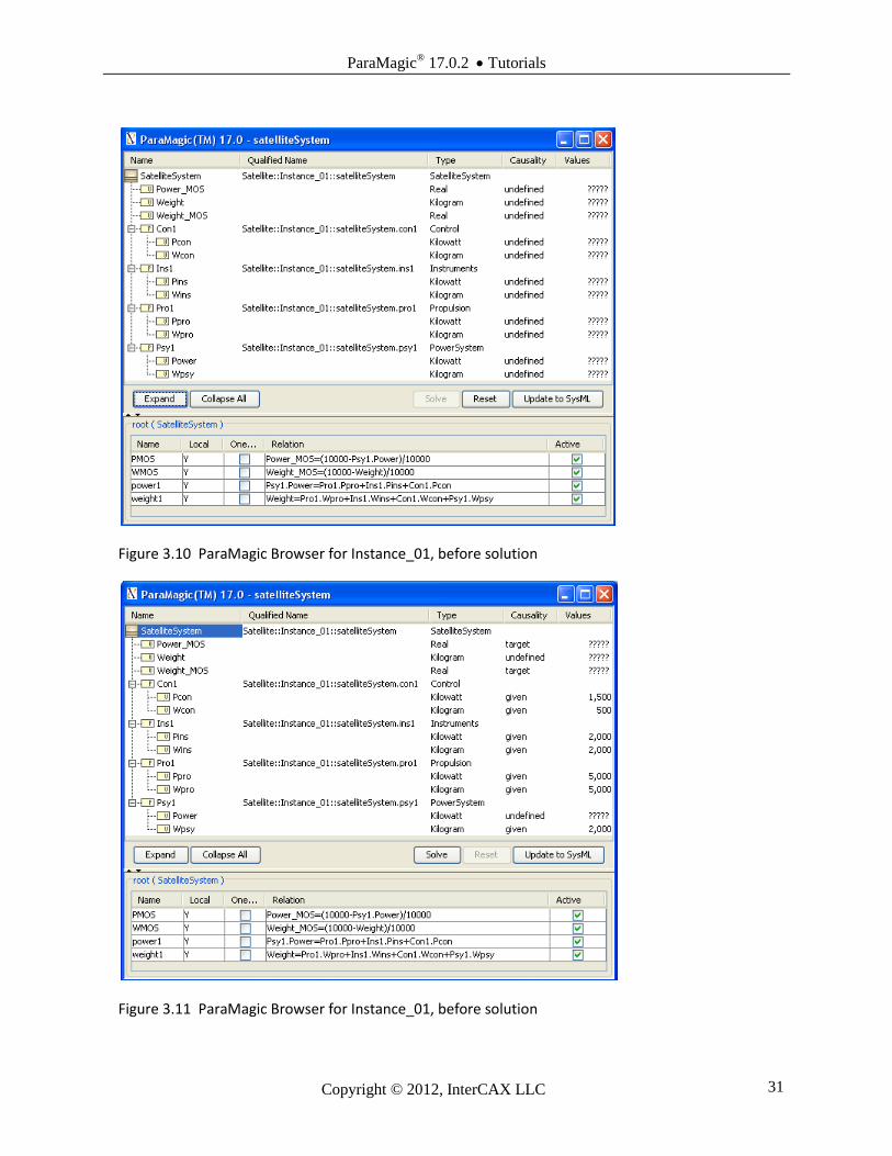
Step VIII Solve the Instance
11. Assign causality and value to all variables.
In this example, we will enter these using
ParaMagic and the browser, rather than
directly into the instances as taught in the
first tutorial.
a. RC on satelliteSystem:Satellite
System (the root instance).
i. Select ParaMagic→Browse.
ii. A message as shown in
Figure 3.9 will appear. This
indicates that no causalities
have been assigned.
iii. Click Reassign. This assigns
undefined casuality to
variables without values
and given causality to
variables with starting
values. At this stage, no
variables have been
assigned a value. The
ParaMagic browser appears
as in Figure 3.10
Figure 3.9 ParaMagic Browser for Instance_01, before solution
b. Assign a given value of 5000 (Kilowatts) to Ppro.
i. Click on the causality assigned to Ppro , initially undefined.
ii. On the pulldown menu that appears, change Ppro’s causality to given.
iii. “InputValue!” appears in the Values column. Change it to 5000.
c. Repeat step c. for all the variables as shown in Figure 3.11. Note that Power_MOS
and Weight_MOS are reassigned to target causality.
Figure 3.8 Satellite Instance_01 Diagram, after wizard
ParaMagic® 17.0.2 Tutorials
Copyright © 2012, InterCAX LLC 31
Figure 3.10 ParaMagic Browser for Instance_01, before solution
Figure 3.11 ParaMagic Browser for Instance_01, before solution
ParaMagic® 17.0.2 Tutorials
Copyright © 2012, InterCAX LLC 32
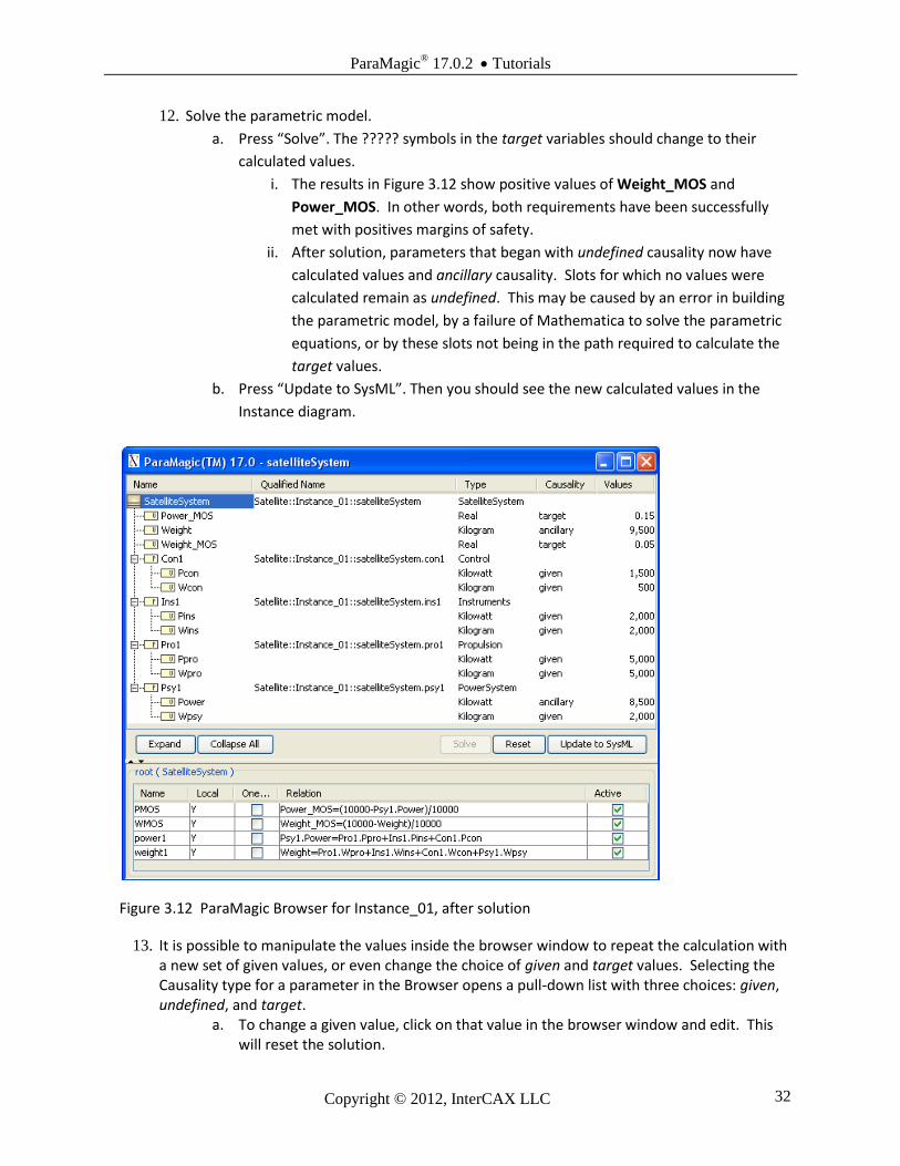
12. Solve the parametric model.
a. Press “Solve”. The ????? symbols in the target variables should change to their
calculated values.
i. The results in Figure 3.12 show positive values of Weight_MOS and
Power_MOS. In other words, both requirements have been successfully
met with positives margins of safety.
ii. After solution, parameters that began with undefined causality now have
calculated values and ancillary causality. Slots for which no values were
calculated remain as undefined. This may be caused by an error in building
the parametric model, by a failure of Mathematica to solve the parametric
equations, or by these slots not being in the path required to calculate the
target values.
b. Press “Update to SysML”. Then you should see the new calculated values in the
Instance diagram.
Figure 3.12 ParaMagic Browser for Instance_01, after solution
13. It is possible to manipulate the values inside the browser window to repeat the calculation with a new set of given values, or even change the choice of given and target values. Selecting the Causality type for a parameter in the Browser opens a pull-down list with three choices: given, undefined, and target.
a. To change a given value, click on that value in the browser window and edit. This will reset the solution.

ParaMagic® 17.0.2 Tutorials
Copyright © 2012, InterCAX LLC 33
b. To change a target or undefined value to a given, or a given value to target or undefined, change the causality for that parameter. In Figure 3.12, the problem has been inverted. “Given the weight budget (10,000 kg) and power budget (10,000 kW) and the properties of the other subsystems, how much weight and power can be allocated to the Instruments subsystem?”. In this example, we set the margins of safety equal to zero and calculate Wins and Pins as targets.
Figure 3.13 ParaMagic Browser for Instance_01, before solution, with changes in causality
Discussion – Causality Mathematica is an “acausal” solver, that is, it can solve many equations in any direction. The user
can take advantage of this to use the same model to answer different kinds of questions. However, not all solvers are acausal (e.g. Microsoft Excel formulas work in one direction only) and not all functions work in multiple directions (e.g. A = MINIMUM(B,C,D) cannot always be solved uniquely for D given A, B and C). Keeping track of causality can require some effort on the part of the modeler.

ParaMagic® 17.0.2 Tutorials
Copyright © 2012, InterCAX LLC 34
4 SYSML PARAMETRICS TUTORIAL - LITTLEEYE
4.1 Objective
The third tutorial concerns using SysML to determine operational performance using a sequence of
equations. The system is the LittleEye unmanned aerial vehicle (UAV) which is used to provide
reconnaissance. The objective is to calculate how many miles of road can be scanned per 24 hours,
which will be determined by the number and duty cycle of aircraft, the number and duty cycle of
crews, and the availability of fuel.
Figure 4.1 Outline of Objective
The complexity of the model, with six elements, eight constraints and more than twenty parameters,
makes it a good place to introduce “object-oriented” modeling techniques, which allow a complex model
to be built from simple, independent and potentially reusable subsystems, tied together only at the highest
levels
What the User Will Learn
Applying an “object-oriented” approach to SysML parametrics
Embedding constraints and parametric diagrams within multiple blocks in the model
Using standard functions, e.g. Minimum
Using simulation to explore a model with “what-if scenarios”
.
ParaMagic® 17.0.2 Tutorials
Copyright © 2012, InterCAX LLC 35
4.2 Step-by-Step Tutorial
Step I Create Project
1. Create new SysML project, Name = LittleEye 2. Create new Package, Name = LittleEye
Step II Create Infrastructure
3. Install ParaMagic Profile module, same as in the Addition tutorial.
Step III Create Structural Model
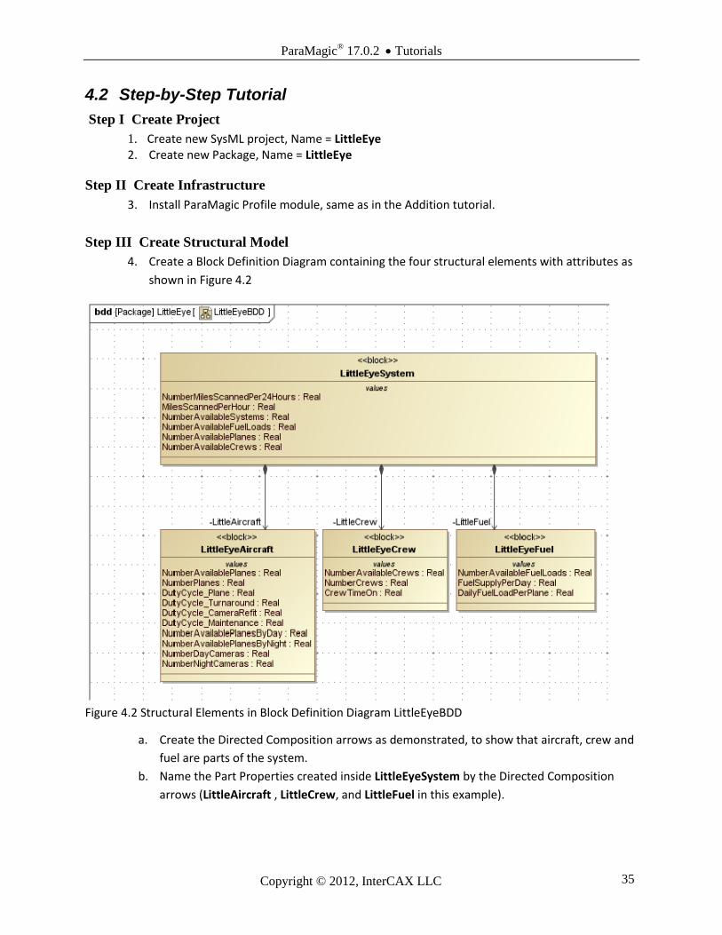
4. Create a Block Definition Diagram containing the four structural elements with attributes as
shown in Figure 4.2
Figure 4.2 Structural Elements in Block Definition Diagram LittleEyeBDD
a. Create the Directed Composition arrows as demonstrated, to show that aircraft, crew and
fuel are parts of the system.
b. Name the Part Properties created inside LittleEyeSystem by the Directed Composition
arrows (LittleAircraft , LittleCrew, and LittleFuel in this example).
ParaMagic® 17.0.2 Tutorials
Copyright © 2012, InterCAX LLC 36
Step IV Create Constraints
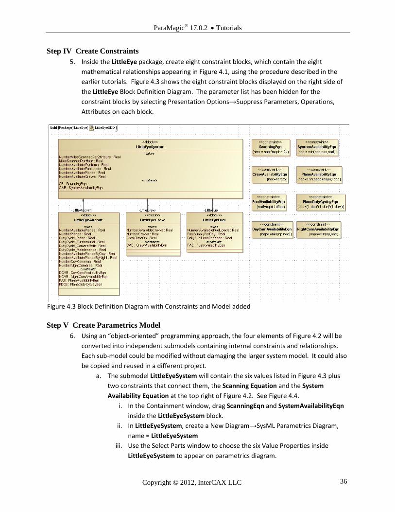
5. Inside the LittleEye package, create eight constraint blocks, which contain the eight
mathematical relationships appearing in Figure 4.1, using the procedure described in the
earlier tutorials. Figure 4.3 shows the eight constraint blocks displayed on the right side of
the LittleEye Block Definition Diagram. The parameter list has been hidden for the
constraint blocks by selecting Presentation Options→Suppress Parameters, Operations,
Attributes on each block.
Figure 4.3 Block Definition Diagram with Constraints and Model added
Step V Create Parametrics Model
6. Using an “object-oriented” programming approach, the four elements of Figure 4.2 will be
converted into independent submodels containing internal constraints and relationships.
Each sub-model could be modified without damaging the larger system model. It could also
be copied and reused in a different project.
a. The submodel LittleEyeSystem will contain the six values listed in Figure 4.3 plus
two constraints that connect them, the Scanning Equation and the System
Availability Equation at the top right of Figure 4.2. See Figure 4.4.
i. In the Containment window, drag ScanningEqn and SystemAvailabilityEqn
inside the LittleEyeSystem block.
ii. In LittleEyeSystem, create a New Diagram→SysML Parametrics Diagram,
name = LittleEyeSystem
iii. Use the Select Parts window to choose the six Value Properties inside
LittleEyeSystem to appear on parametrics diagram.
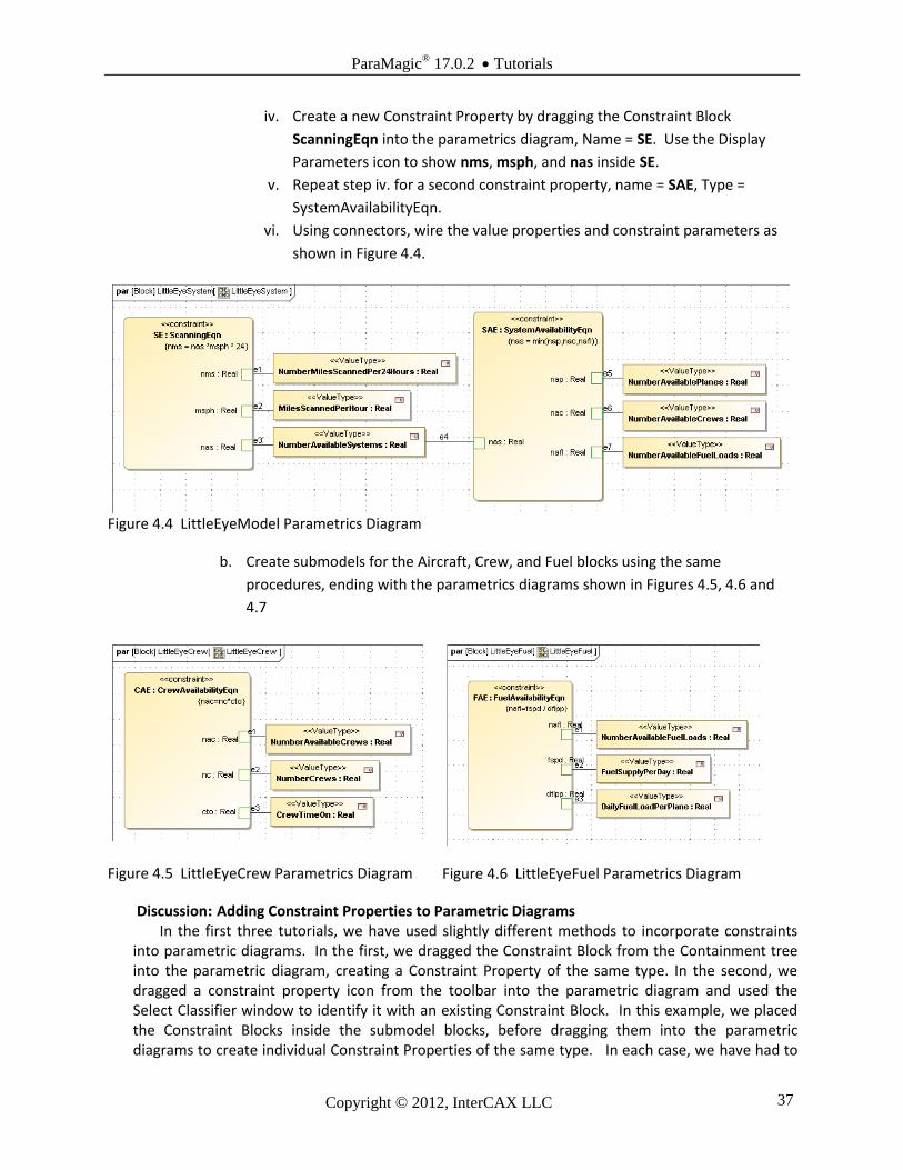
ParaMagic® 17.0.2 Tutorials
Copyright © 2012, InterCAX LLC 37
iv. Create a new Constraint Property by dragging the Constraint Block
ScanningEqn into the parametrics diagram, Name = SE. Use the Display
Parameters icon to show nms, msph, and nas inside SE.
v. Repeat step iv. for a second constraint property, name = SAE, Type =
SystemAvailabilityEqn.
vi. Using connectors, wire the value properties and constraint parameters as
shown in Figure 4.4.
Figure 4.4 LittleEyeModel Parametrics Diagram
b. Create submodels for the Aircraft, Crew, and Fuel blocks using the same
procedures, ending with the parametrics diagrams shown in Figures 4.5, 4.6 and
4.7
Figure 4.5 LittleEyeCrew Parametrics Diagram Figure 4.6 LittleEyeFuel Parametrics Diagram
Discussion: Adding Constraint Properties to Parametric Diagrams In the first three tutorials, we have used slightly different methods to incorporate constraints
into parametric diagrams. In the first, we dragged the Constraint Block from the Containment tree into the parametric diagram, creating a Constraint Property of the same type. In the second, we dragged a constraint property icon from the toolbar into the parametric diagram and used the Select Classifier window to identify it with an existing Constraint Block. In this example, we placed the Constraint Blocks inside the submodel blocks, before dragging them into the parametric diagrams to create individual Constraint Properties of the same type. In each case, we have had to

ParaMagic® 17.0.2 Tutorials
Copyright © 2012, InterCAX LLC 38
assign the Constraint Property created a unique name. All three methods work. The third implies an exclusive ownership of the constraint by a
particular submodel, which may be misleading if the constraint block is to be re-used by other parts of model. Assigning ownership may be useful in a collaborative environment, but it is also OK to keep Constraint Blocks anywhere in the project, e.g. in a Constraints library, and drag them into specific parametric diagrams as needed.
Figure 4.7 LittleEyeAircraft Parametrics Diagram
7. It is also necessary to create an overall parametric diagram to connect the different
submodels. This is an objective of “object-oriented” programming, to create independent
modules and link them in the simplest possible way. Within the top-level block, LittleEye
System, several properties have been created with the same names as properties in the
lower-level models, e.g. NumberAvailablePlanes. In the following steps, we use connectors
to link models together through these duplicate parameters. (Alternate: the duplicate
parameters could also be linked using explicit equality constraint relationships, created as
an Equality constraint block in Step 8 and used three times within this parametric diagram.
However, this involves a lot of extra work. ParaMagic interprets direct connections between
value properties as equality relationships).
a. Create a second SysML Parametrics diagram inside LittleEyeSystem called
LittleEyeSystem_2.
b. Use the Select Parts window to select the Part Properties LittleAircraft, LittleCrew
and LittleFuel, to appear in the parametrics diagram.
ParaMagic® 17.0.2 Tutorials
Copyright © 2012, InterCAX LLC 39
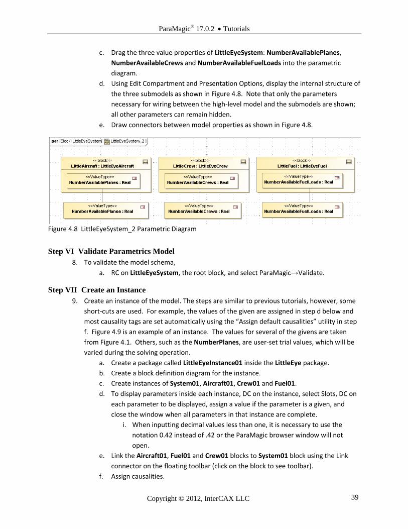
c. Drag the three value properties of LittleEyeSystem: NumberAvailablePlanes,
NumberAvailableCrews and NumberAvailableFuelLoads into the parametric
diagram.
d. Using Edit Compartment and Presentation Options, display the internal structure of
the three submodels as shown in Figure 4.8. Note that only the parameters
necessary for wiring between the high-level model and the submodels are shown;
all other parameters can remain hidden.
e. Draw connectors between model properties as shown in Figure 4.8.
Figure 4.8 LittleEyeSystem_2 Parametric Diagram
Step VI Validate Parametrics Model
8. To validate the model schema,
a. RC on LittleEyeSystem, the root block, and select ParaMagic→Validate.
Step VII Create an Instance
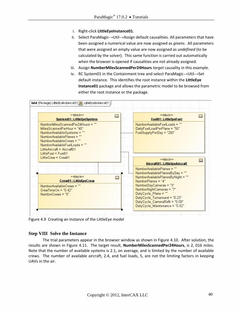
9. Create an instance of the model. The steps are similar to previous tutorials, however, some
short-cuts are used. For example, the values of the given are assigned in step d below and
most causality tags are set automatically using the “Assign default causalities” utility in step
f. Figure 4.9 is an example of an instance. The values for several of the givens are taken
from Figure 4.1. Others, such as the NumberPlanes, are user-set trial values, which will be
varied during the solving operation.
a. Create a package called LittleEyeInstance01 inside the LittleEye package.
b. Create a block definition diagram for the instance.
c. Create instances of System01, Aircraft01, Crew01 and Fuel01.
d. To display parameters inside each instance, DC on the instance, select Slots, DC on
each parameter to be displayed, assign a value if the parameter is a given, and
close the window when all parameters in that instance are complete.
i. When inputting decimal values less than one, it is necessary to use the
notation 0.42 instead of .42 or the ParaMagic browser window will not
open.
e. Link the Aircraft01, Fuel01 and Crew01 blocks to System01 block using the Link
connector on the floating toolbar (click on the block to see toolbar).
f. Assign causalities.
ParaMagic® 17.0.2 Tutorials
Copyright © 2012, InterCAX LLC 40
i. Right-click LittleEyeInstance01.
ii. Select ParaMagic→Util→Assign default causalities. All parameters that have
been assigned a numerical value are now assigned as givens. All parameters
that were assigned an empty value are now assigned as undefined (to be
calculated by the solver). This same function is carried out automatically
when the browser is opened if causalities are not already assigned.
iii. Assign NumberMilesScannedPer24Hours target causality in this example.
iv. RC System01 in the Containment tree and select ParaMagic→Util→Set
default instance. This identifies the root instance within the LittleEye
Instance01 package and allows the parametric model to be browsed from
either the root instance or the package.
Figure 4.9 Creating an Instance of the LittleEye model
Step VIII Solve the Instance
The trial parameters appear in the browser window as shown in Figure 4.10. After solution, the results are shown in Figure 4.11. The target result, NumberMilesScannedPer24Hours, is 2, 016 miles. Note that the number of available systems is 2.1, on average, and is limited by the number of available crews. The number of available aircraft, 2.4, and fuel loads, 5, are not the limiting factors in keeping UAVs in the air.

ParaMagic® 17.0.2 Tutorials
Copyright © 2012, InterCAX LLC 41
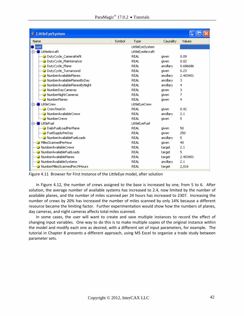
In Figure 4.11, several parameters are labeled “ancillary” after solution. This implies that they were
calculated during the solution process, and were used in further calculations. For example, the number of available crews was calculated from the number of crews and the crew duty cycle, and is used in calculating the number of available systems.
Figure 4.10 Browser for First Instance of the LittleEye model, before Solution
ParaMagic® 17.0.2 Tutorials
Copyright © 2012, InterCAX LLC 42
Figure 4.11 Browser for First Instance of the LittleEye model, after solution
In Figure 4.12, the number of crews assigned to the base is increased by one, from 5 to 6. After solution, the average number of available systems has increased to 2.4, now limited by the number of available planes, and the number of miles scanned per 24 hours has increased to 2307. Increasing the number of crews by 20% has increased the number of miles scanned by only 14% because a different resource became the limiting factor. Further experimentation would show how the numbers of planes, day cameras, and night cameras affects total miles scanned.
In some cases, the user will want to create and save multiple instances to record the effect of changing input variables. One way to do this is to make multiple copies of the original instance within the model and modify each one as desired, with a different set of input parameters, for example. The tutorial in Chapter 8 presents a different approach, using MS Excel to organize a trade study between parameter sets.

ParaMagic® 17.0.2 Tutorials
Copyright © 2012, InterCAX LLC 43
Figure 4.12 Browser for Second Instance of the LittleEye model, NumberCrews increased by one, after solution

ParaMagic® 17.0.2 Tutorials
Copyright © 2012, InterCAX LLC 44
5 SYSML PARAMETRICS TUTORIAL - COMMNETWORK
5.1 Objective
The fourth tutorial uses SysML to simulate a simple communication network. The objective is to
calculate the output of the network given the input and the loss in the individual channels between
stations..
Figure 5.1 Outline of Network
The focus of this tutorial is working with limited number of standard elements to build up more complex
structures. In this example, there are only two standard elements, stations (nodes) and channels. Each
element contains constraint relations describing its behavior. An Internal Block Diagram is created to
assist in completing the parametric diagrams correctly. Parametric constraints are also used at a higher
level to define interactions between elements.
What the User Will Learn
Building complex structures from multiple usages of simple structures
Using internal block diagrams
5.2 Step-by-Step Tutorial
Step I Create Project
1. Create new SysML project and Package, Name = CommNetwork
Step II Create Infrastructure
2. Install ParaMagic Profile module, same as in first tutorial.
ParaMagic® 17.0.2 Tutorials
Copyright © 2012, InterCAX LLC 45
Step III Create Structural Model
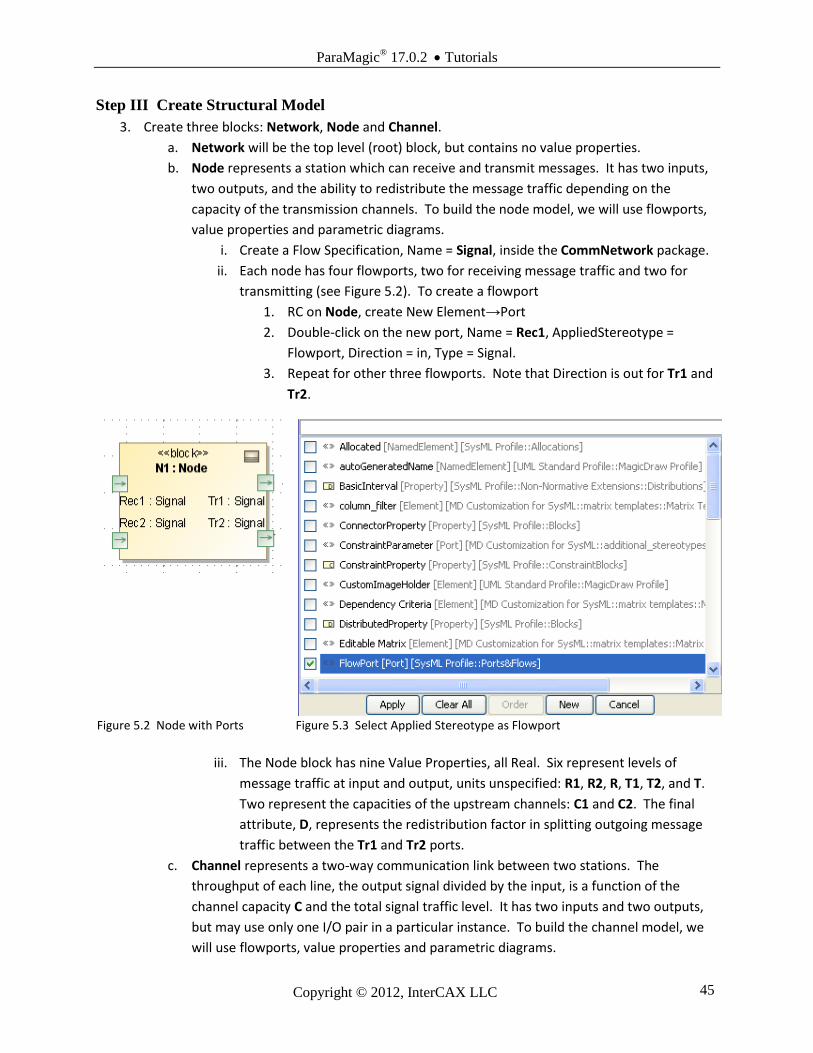
3. Create three blocks: Network, Node and Channel.
a. Network will be the top level (root) block, but contains no value properties.
b. Node represents a station which can receive and transmit messages. It has two inputs,
two outputs, and the ability to redistribute the message traffic depending on the
capacity of the transmission channels. To build the node model, we will use flowports,
value properties and parametric diagrams.
i. Create a Flow Specification, Name = Signal, inside the CommNetwork package.
ii. Each node has four flowports, two for receiving message traffic and two for
transmitting (see Figure 5.2). To create a flowport
1. RC on Node, create New Element→Port
2. Double-click on the new port, Name = Rec1, AppliedStereotype =
Flowport, Direction = in, Type = Signal.
3. Repeat for other three flowports. Note that Direction is out for Tr1 and
Tr2.
Figure 5.2 Node with Ports Figure 5.3 Select Applied Stereotype as Flowport
iii. The Node block has nine Value Properties, all Real. Six represent levels of
message traffic at input and output, units unspecified: R1, R2, R, T1, T2, and T.
Two represent the capacities of the upstream channels: C1 and C2. The final
attribute, D, represents the redistribution factor in splitting outgoing message
traffic between the Tr1 and Tr2 ports.
c. Channel represents a two-way communication link between two stations. The
throughput of each line, the output signal divided by the input, is a function of the
channel capacity C and the total signal traffic level. It has two inputs and two outputs,
but may use only one I/O pair in a particular instance. To build the channel model, we
will use flowports, value properties and parametric diagrams.
ParaMagic® 17.0.2 Tutorials
Copyright © 2012, InterCAX LLC 46
i. Each channel has four flowports, two for input message traffic and two for
output (see Channel blocks in Figure 5.6). To create a flowport
1. RC on Channel, create New Element→Port
2. Double-click on the new port, Name = In1, AppliedStereotype =
Flowport, Direction = in, Type = Signal.
3. Repeat for other three flowports. Note that Direction is out for Out1
and Out2.
ii. The Channel block has six Value Properties, all Real. Five represent levels of
message traffic at input and output, units unspecified: IT1, IT2, IT, 0T1, and 0T2.
C represents the intrinsic capacity of the channel.
4. Create a Block Definition Diagram and an Internal Block Diagram
a. RC on CommNetwork package, create New Diagram→SysML Diagrams→SysML Block
Definition Diagram, Name = Network_BDD
i. Drag Network, Node and Channel blocks into the diagram
ii. Using the Direct Composition connector from the floating toolbar, connect as
shown in Figure 5.4. Note that four connections are made from Network to a
single Node block, and the resulting four Part Properties are named N1, N2, N3
and N4. Similarly, five connections are made from Network to a single Channel
block, named as ChA thru ChE.
Figure 5.4 CommNetwork Block Definition Diagram
ParaMagic® 17.0.2 Tutorials
Copyright © 2012, InterCAX LLC 47
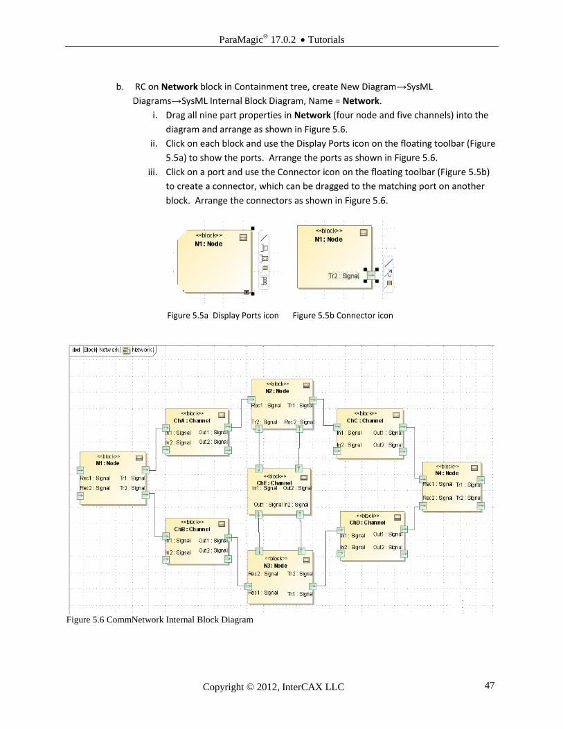
b. RC on Network block in Containment tree, create New Diagram→SysML
Diagrams→SysML Internal Block Diagram, Name = Network.
i. Drag all nine part properties in Network (four node and five channels) into the
diagram and arrange as shown in Figure 5.6.
ii. Click on each block and use the Display Ports icon on the floating toolbar (Figure
5.5a) to show the ports. Arrange the ports as shown in Figure 5.6.
iii. Click on a port and use the Connector icon on the floating toolbar (Figure 5.5b)
to create a connector, which can be dragged to the matching port on another
block. Arrange the connectors as shown in Figure 5.6.
Figure 5.5a Display Ports icon Figure 5.5b Connector icon
Figure 5.6 CommNetwork Internal Block Diagram
ParaMagic® 17.0.2 Tutorials
Copyright © 2012, InterCAX LLC 48
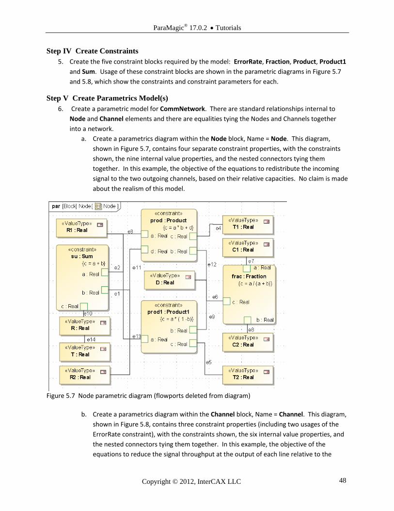
Step IV Create Constraints
5. Create the five constraint blocks required by the model: ErrorRate, Fraction, Product, Product1
and Sum. Usage of these constraint blocks are shown in the parametric diagrams in Figure 5.7
and 5.8, which show the constraints and constraint parameters for each.
Step V Create Parametrics Model(s)
6. Create a parametric model for CommNetwork. There are standard relationships internal to
Node and Channel elements and there are equalities tying the Nodes and Channels together
into a network.
a. Create a parametrics diagram within the Node block, Name = Node. This diagram,
shown in Figure 5.7, contains four separate constraint properties, with the constraints
shown, the nine internal value properties, and the nested connectors tying them
together. In this example, the objective of the equations to redistribute the incoming
signal to the two outgoing channels, based on their relative capacities. No claim is made
about the realism of this model.
Figure 5.7 Node parametric diagram (flowports deleted from diagram)
b. Create a parametrics diagram within the Channel block, Name = Channel. This diagram,
shown in Figure 5.8, contains three constraint properties (including two usages of the
ErrorRate constraint), with the constraints shown, the six internal value properties, and
the nested connectors tying them together. In this example, the objective of the
equations to reduce the signal throughput at the output of each line relative to the
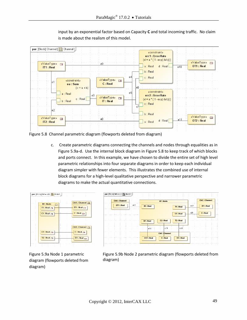
ParaMagic® 17.0.2 Tutorials
Copyright © 2012, InterCAX LLC 49
input by an exponential factor based on Capacity C and total incoming traffic. No claim
is made about the realism of this model.
Figure 5.8 Channel parametric diagram (flowports deleted from diagram)
c. Create parametric diagrams connecting the channels and nodes through equalities as in
Figure 5.9a-d. Use the internal block diagram in Figure 5.8 to keep track of which blocks
and ports connect. In this example, we have chosen to divide the entire set of high level
parametric relationships into four separate diagrams in order to keep each individual
diagram simpler with fewer elements. This illustrates the combined use of internal
block diagrams for a high-level qualitative perspective and narrower parametric
diagrams to make the actual quantitative connections.
Figure 5.9a Node 1 parametric
diagram (flowports deleted from
diagram)
Figure 5.9b Node 2 parametric diagram (flowports deleted from diagram)
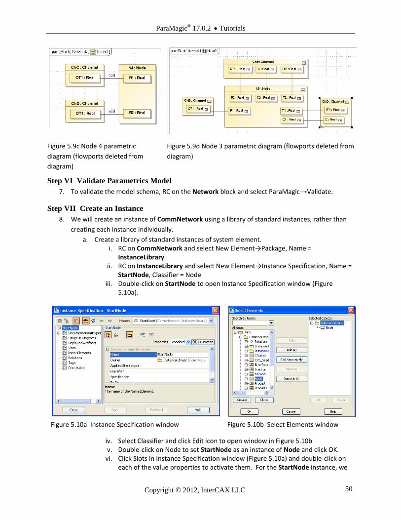
ParaMagic® 17.0.2 Tutorials
Copyright © 2012, InterCAX LLC 50
Figure 5.9c Node 4 parametric
diagram (flowports deleted from
diagram)
Figure 5.9d Node 3 parametric diagram (flowports deleted from
diagram)
Step VI Validate Parametrics Model
7. To validate the model schema, RC on the Network block and select ParaMagic→Validate.
Step VII Create an Instance
8. We will create an instance of CommNetwork using a library of standard instances, rather than
creating each instance individually.
a. Create a library of standard instances of system element. i. RC on CommNetwork and select New Element→Package, Name =
InstanceLibrary ii. RC on InstanceLibrary and select New Element→Instance Specification, Name =
StartNode, Classifier = Node iii. Double-click on StartNode to open Instance Specification window (Figure
5.10a).
Figure 5.10a Instance Specification window Figure 5.10b Select Elements window
iv. Select Classifier and click Edit icon to open window in Figure 5.10b v. Double-click on Node to set StartNode as an instance of Node and click OK.
vi. Click Slots in Instance Specification window (Figure 5.10a) and double-click on each of the value properties to activate them. For the StartNode instance, we

ParaMagic® 17.0.2 Tutorials
Copyright © 2012, InterCAX LLC 51
assume a given input signal level by assigning R1 as 10 (arbitrary units) and R2 as 0. All the remaining slots are left empty. Click Close at the end.
vii. Repeat this process for four more standard instances: 1. ThruNode (stations which both receive from and transmit to other
stations in the network). All slots are activated, but left empty. 2. EndNode (stations which only receive, i.e. final destination). Assign C1
and C2 values = 1 or any non-zero fixed value because there are no “downstream” channels to supply these values.
3. SingleChannel (channels in which only one I/O path is used). Classifier = Channel. Assign C = 5 (capacity in arbitrary units) and IT2 = 0 because input to second I/O path is not used.
4. DoubleChannel (channels in which both I/O paths are used). Classifier = Channel. Assign C = 5 (capacity in arbitrary units).
viii. Assign causality to all standard instances by right-clicking on
InstanceLibrary and selecting ParaMagic→Util→Assign default
causalities.
ix. The final contents of InstanceLibrary should appear as in
Figure 5.11. Any of these instances can be dragged into an
instance diagram in another package and used without further
modification.
b. Create a specific instance package for the network proposed
i. RC on CommNetwork and select New Element→Package, Name = Instance01 ii. RC on Instance01 and select New Diagram→SysML Diagrams→SysML Block
Definition Diagram, Name = Instance01.
iii. We need four separate copies of SingleChannel in our
network, to represent Channels A, B, C, and D. In this example,
we will copy SingleChannel and paste four copies into
Instance01, named SingleChanne0, SingleChannel1,
SingleChannel2 and SingleChannel3.
iv. We need two separate copies of ThruNode in our network,
to represent Nodes 2 and 3. In this example, we will copy
ThruNode and paste two copies into Instance01, named
ThruNode0 and ThruNode1.
v. We need copies of DoubleChannel, StartNode and
EndNode in Instance01.
vi. Finally, create an instance of the Network block inside
Instance01, Name = Net0. The final contents of Instance01
should appear as in Figure 5.12
vii. Drag all the instances in Instance01 into the Instance01
diagram.
Figure 5.11 InstanceLibrary contents
Figure 5.12 Instance01 contents
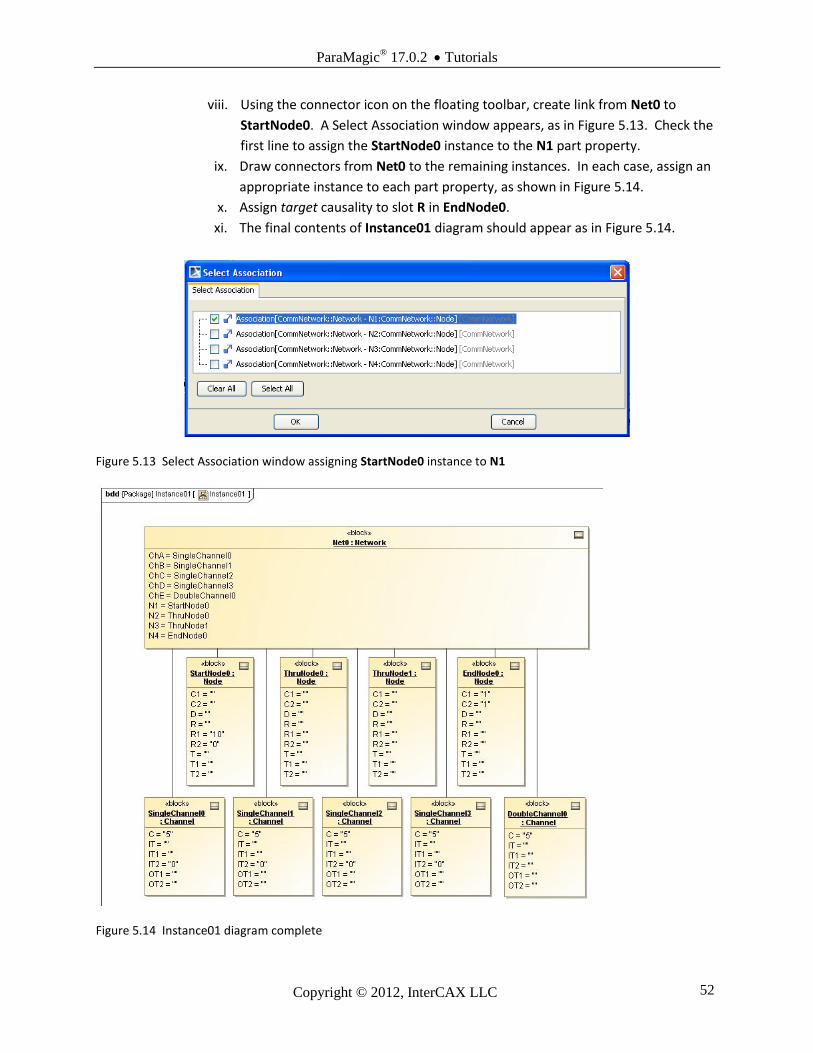
ParaMagic® 17.0.2 Tutorials
Copyright © 2012, InterCAX LLC 52
viii. Using the connector icon on the floating toolbar, create link from Net0 to
StartNode0. A Select Association window appears, as in Figure 5.13. Check the
first line to assign the StartNode0 instance to the N1 part property.
ix. Draw connectors from Net0 to the remaining instances. In each case, assign an
appropriate instance to each part property, as shown in Figure 5.14.
x. Assign target causality to slot R in EndNode0.
xi. The final contents of Instance01 diagram should appear as in Figure 5.14.
Figure 5.13 Select Association window assigning StartNode0 instance to N1
Figure 5.14 Instance01 diagram complete

ParaMagic® 17.0.2 Tutorials
Copyright © 2012, InterCAX LLC 53
Discussion – Instance Generation We have used four different methods for creating instance in our first four tutorials,
Creating individual instances from the central toolbar
Creating individual instances using menu commands
Using the Instance Generation Wizard
Copying and pasting existing instances from a standard instance library Similarly, there are at least two ways of linking instances,
Draw a link from the higher block to the lower and use the Select Association window to assign the instance to an existing part property.
Double-click on the higher block, click on Slots, double-click on a part property, and assign it to an existing instance. In this approach, no visible line connects the instances on the instance diagram, but the higher-level instance box displays the association, e.g. ChE = DoubleChannel0.
Which method to choose depends on the situation. Being familiar with multiple approaches is advantageous.
Step VIII Solve the Instance
9. In Figures 5.15 and 5.16, only a few of the output variables are expanded to display. All of the
values are available, however.
Figure 5.15 Browser for Instance01 before solution Figure 5.16 Browser for Instance01 after solution
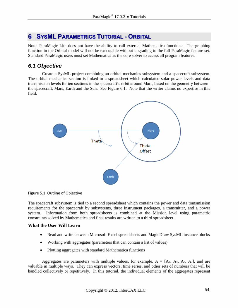
ParaMagic® 17.0.2 Tutorials
Copyright © 2012, InterCAX LLC 54
6 SYSML PARAMETRICS TUTORIAL - ORBITAL
Note: ParaMagic Lite does not have the ability to call external Mathematica functions. The graphing
function in the Orbital model will not be executable without upgrading to the full ParaMagic feature set.
Standard ParaMagic users must set Mathematica as the core solver to access all program features.
6.1 Objective
Create a SysML project combining an orbital mechanics subsystem and a spacecraft subsystem.
The orbital mechanics section is linked to a spreadsheet which calculated solar power levels and data
transmission levels for ten sections in the spacecraft’s orbit around Mars, based on the geometry between
the spacecraft, Mars, Earth and the Sun. See Figure 6.1. Note that the writer claims no expertise in this
field.
Figure 5.1 Outline of Objective
The spacecraft subsystem is tied to a second spreadsheet which contains the power and data transmission
requirements for the spacecraft by subsystems, three instrument packages, a transmitter, and a power
system. Information from both spreadsheets is combined at the Mission level using parametric
constraints solved by Mathematica and final results are written to a third spreadsheet.
What the User Will Learn
Read and write between Microsoft Excel spreadsheets and MagicDraw SysML instance blocks
Working with aggregates (parameters that can contain a list of values)
Plotting aggregates with standard Mathematica functions
Aggregates are parameters with multiple values, for example, A = [A1, A2, A3, A4], and are
valuable in multiple ways. They can express vectors, time series, and other sets of numbers that will be
handled collectively or repetitively. In this tutorial, the individual elements of the aggregates represent
ParaMagic® 17.0.2 Tutorials
Copyright © 2012, InterCAX LLC 55
values for ten separate sections of the orbital cycle. The specific number of elements does not need to be
defined until the instance stage.
Mathematica has extensive graphics capability. Graphs can be created and saved during
ParaMagic execution, using several ParaMagic-provided standard functions. User-created Mathematica
functions, described in the ParaMagic Users Guide, provide even more flexibility.
Spreadsheets, such as Microsoft Excel, could be envisioned either as a means of loading data into
a specific instance from an existing table or database, a means of reporting and organizing results from a
parametric simulation, or a mathematical solver for parametric relationships that are part of the model.
Currently, ParaMagic only supports the first two functions.
System Requirements
Microsoft Excel 2003 or 2007. Note: Excel is not required to execute the ParaMagic-Excel
interface. It is required to create, edit and view the spreadsheets used in the example.
In order to use standard Mathematica functions that produce a graphics file, Mathematica must
be loaded on the user’s local machine or server (no web services) and the ICAX standard
function library must be installed for autoloading.
6.2 Step-by Step Tutorial
Step I Create Project
1. Create new project
c. Name = Orbital
2. Create a package within the project
a. RC (Right-click) on Data folder in Containment tree (left column)
b. Choose New Element→Package
c. Enter Name = Orbital
Step II Create Infrastructure
3. Install ParaMagic Profile module, same as in the first tutorial.
Step III Create Structural Model
4. Create elements in model
a. Inside the Orbital package, create blocks called Mission, Orbital, Spacecraft,
InPkg1, InPkg2, InPkg3, Transmitter, and PowerSystem.
b. Create a block definition diagram, Name = Mission, and drag the Orbital elements
into the diagram. See Figure 6.2. Use Directed Composition connectors to link the
blocks in the hierarchy shown.
c. Inside Mission, create a value property called AveragePowerWindow and assign it
a Type as Real. Repeat this procedure for three additional properties in Mission:
AverageXmitWindow, EffectivePowerBudget, and EffectiveXmitBudget.
d. Referring to Figure 6.2, create value properties as shown in the Spacecraft, InPkg1,
InPkg2, InPkg3, Transmitter, and PowerSystem blocks, all type Real.
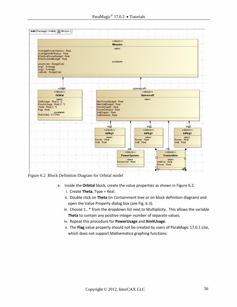
ParaMagic® 17.0.2 Tutorials
Copyright © 2012, InterCAX LLC 56
e. Inside the Orbital block, create the value properties as shown in Figure 6.2.
i. Create Theta, Type = Real.
ii. Double click on Theta (in Containment tree or on block definition diagram) and
open the Value Property dialog box (see Fig. 6.3).
iii. Choose 1…* from the dropdown list next to Multiplicity. This allows the variable
Theta to contain any positive integer number of separate values.
iv. Repeat this procedure for PowerUsage and XmitUsage.
v. The Flag value property should not be created by users of ParaMagic 17.0.1 Lite,
which does not support Mathematica graphing functions.
Figure 6.2 Block Definition Diagram for Orbital model

ParaMagic® 17.0.2 Tutorials
Copyright © 2012, InterCAX LLC 57
Step IV Create Constraints
5. Create two constraint blocks, Average
and BudgetCalc, as shown in Figure
6.4. Note that Average uses list, a
constraint parameter with multiplicity
larger than one. To change the
multiplicity of a constraint parameter,
RC the constraint block in the BDD
diagram. Average calculates the
average of all the values contained in
list and returns a single value result,
mean. The ParaMagic User Guide
provides a list of Mathematica
functions that act on arguments with
multiplicity > 1.
6. Create a constraint block for plotting
the power and transmission availability versus Theta. Users of ParaMagic 17.0.1 Lite will not be
able to execute this graphing function and should skip step 6 a-d.
a. See User Guide for a list of standard Mathematica graphics and statistical functions that
are provided with ParaMagic. These should be configured to automatically load when
Mathematica is started.
Figure 6.3 Setting the value property Theta multiplicity to 1…*
Fig. 6.4 Constraint Blocks
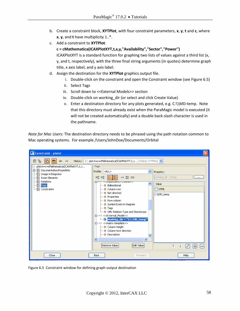
ParaMagic® 17.0.2 Tutorials
Copyright © 2012, InterCAX LLC 58
b. Create a constraint block, XYTPlot, with four constraint parameters, x, y, t and c, where
x, y, and t have multiplicity 1..*.
c. Add a constraint to XYTPlot.
c = cMathematica(ICAXPlotXYT,t,x,y,"Availability","Sector","Power")
ICAXPlotXYT is a standard function for graphing two lists of values against a third list (x,
y, and t, respectively), with the three final string arguments (in quotes) determine graph
title, x axis label, and y axis label.
d. Assign the destination for the XYTPlot graphics output file.
i. Double-click on the constraint and open the Constraint window (see Figure 6.5)
ii. Select Tags
iii. Scroll down to <<External Models>> section
iv. Double-click on working_dir (or select and click Create Value)
v. Enter a destination directory for any plots generated, e.g. C:\\MD-temp. Note
that this directory must already exist when the ParaMagic model is executed (it
will not be created automatically) and a double back-slash character is used in
the pathname.
Note for Mac Users: The destination directory needs to be phrased using the path notation common to
Mac operating systems. For example /Users/JohnDoe/Documents/Orbital
Figure 6.5 Constraint window for defining graph output destination
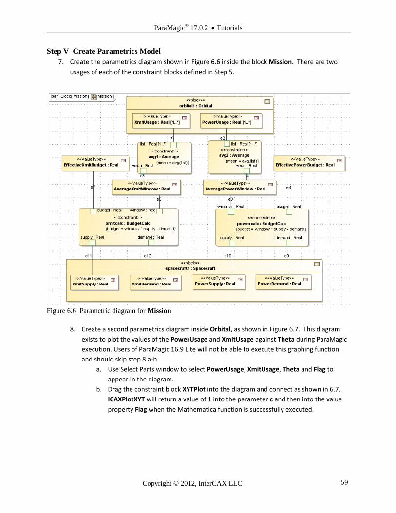
ParaMagic® 17.0.2 Tutorials
Copyright © 2012, InterCAX LLC 59
Step V Create Parametrics Model
7. Create the parametrics diagram shown in Figure 6.6 inside the block Mission. There are two
usages of each of the constraint blocks defined in Step 5.
8. Create a second parametrics diagram inside Orbital, as shown in Figure 6.7. This diagram
exists to plot the values of the PowerUsage and XmitUsage against Theta during ParaMagic
execution. Users of ParaMagic 16.9 Lite will not be able to execute this graphing function
and should skip step 8 a-b.
a. Use Select Parts window to select PowerUsage, XmitUsage, Theta and Flag to
appear in the diagram.
b. Drag the constraint block XYTPlot into the diagram and connect as shown in 6.7.
ICAXPlotXYT will return a value of 1 into the parameter c and then into the value
property Flag when the Mathematica function is successfully executed.
Figure 6.6 Parametric diagram for Mission

ParaMagic® 17.0.2 Tutorials
Copyright © 2012, InterCAX LLC 60
Step VI Validate Parametrics Model
9. To validate the model schema, follow the instructions in Step VI of previous tutorials
Step VII Create an Instance
In this example, we will create an instance of the SysML model and three separate Microsoft Excel spreadsheets that will link to this instance and allow data to be written from Excel to MagicDraw SysML and from MagicDraw SysML to Excel. This supports the use of spreadsheets to load data into a model and to report results from parametric simulation of the model. In normal circumstances, some or all of these spreadsheets may exist prior to the SysML model, but in this tutorial, we will create them at this stage.
10. Create three workbooks in Microsoft Excel that instances of the model will link to.
a. Open Excel and create and save the workbook spacecraft (.xls or .xlsx) shown in Figure
6.8 (in worksheet Sheet1).
Figure 6.8a Workbook spacecraft, showing values
Figure 6.8b Workbook spacecraft, showing formulas
b. Build and save the spreadsheet orbital shown in Figure 6.9 (in worksheet Sheet1).
Figure 6.7 Parametric diagram for Orbital
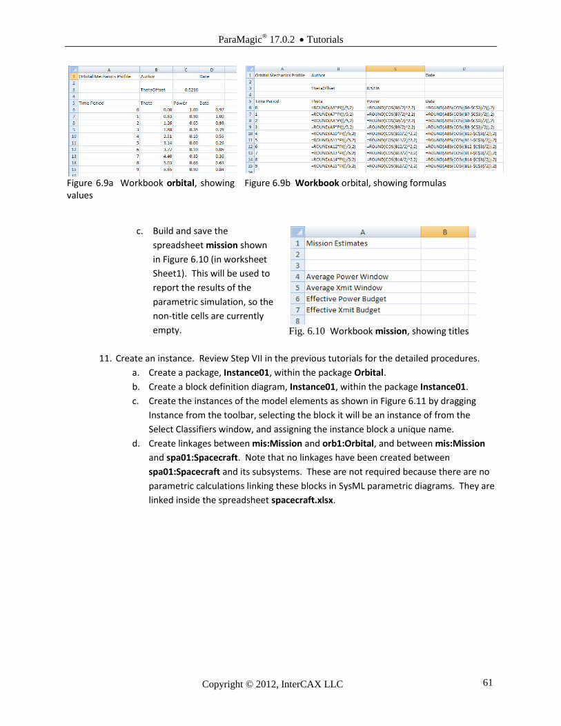
ParaMagic® 17.0.2 Tutorials
Copyright © 2012, InterCAX LLC 61
Figure 6.9a Workbook orbital, showing values
Figure 6.9b Workbook orbital, showing formulas
c. Build and save the
spreadsheet mission shown
in Figure 6.10 (in worksheet
Sheet1). This will be used to
report the results of the
parametric simulation, so the
non-title cells are currently
empty.
11. Create an instance. Review Step VII in the previous tutorials for the detailed procedures.
a. Create a package, Instance01, within the package Orbital.
b. Create a block definition diagram, Instance01, within the package Instance01.
c. Create the instances of the model elements as shown in Figure 6.11 by dragging
Instance from the toolbar, selecting the block it will be an instance of from the
Select Classifiers window, and assigning the instance block a unique name.
d. Create linkages between mis:Mission and orb1:Orbital, and between mis:Mission
and spa01:Spacecraft. Note that no linkages have been created between
spa01:Spacecraft and its subsystems. These are not required because there are no
parametric calculations linking these blocks in SysML parametric diagrams. They are
linked inside the spreadsheet spacecraft.xlsx.
Fig. 6.10 Workbook mission, showing titles
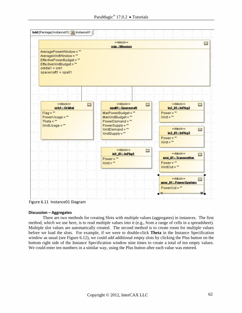
ParaMagic® 17.0.2 Tutorials
Copyright © 2012, InterCAX LLC 62
Figure 6.11 Instance01 Diagram Discussion – Aggregates
There are two methods for creating Slots with multiple values (aggregates) in instances. The first
method, which we use here, is to read multiple values into it (e.g., from a range of cells in a spreadsheet).
Multiple slot values are automatically created. The second method is to create room for multiple values
before we load the slots. For example, if we were to double-click Theta in the Instance Specification
window as usual (see Figure 6.12), we could add additional empty slots by clicking the Plus button on the
bottom right side of the Instance Specification window nine times to create a total of ten empty values.
We could enter ten numbers in a similar way, using the Plus button after each value was entered.
ParaMagic® 17.0.2 Tutorials
Copyright © 2012, InterCAX LLC 63
12. Create the connection between the spacecraft instance blocks and spreadsheet
spacecraft.xlsx.
a. In the Containment window, right-click on the instance block In1_01 and select
ParaMagic→Excel→Setup.
b. The ParaMagic-Excel Setup window will appear as in Figure 6.13a. The spreadsheet
to be linked can be identified in two ways
i. Browse to the desired file. This will enter the full path name in the
Workbook file text box, or
ii. Type in the filename, e.g. spacecraft.xlsx and click Refresh. If no path is
typed, it will assume spreadsheet is in the same folder as the model (.mdzip
file). This may be more flexible if the model and spreadsheet are moved
around between different systems.
c. After the Workbook name is entered and the Refresh button is clicked, the
available worksheets within that file will appear as a drop-down list by the
Worksheet name label. Select the desired worksheet, Sheet1. See Figure 6.13b.
Figure 6.12 Assigning ten empty values to the Theta parameter in orb1

ParaMagic® 17.0.2 Tutorials
Copyright © 2012, InterCAX LLC 64
Figure 6.13a ParaMagic- Excel Set-up for instance
Figure 6.13b ParaMagic- Excel Set-up for instance after completion
d. In the Excel Setup browser, select the Power slot. See Figure 6.14.
i. Under Cell Range, enter the cell coordinates on the spreadsheet for the
parameter desired, B3.
ii. Under Access Mode, select Read (the value in the spreadsheet cell will be
copied to the instance, though only after we transfer the data in step 14).
iii. Repeat for Xmit. The corresponding Cell range is C3.
iv. Click OK
Figure 6.14 ParaMagic- Excel Set-up for slot
Figure 6.15 ParaMagic- Excel Set-up for slot
e. Repeat steps d, e, and f for the remainder of the
instance blocks in the diagram.
i. For slots where we will write the result
from the SysML model to the mission.xlsx
spreadsheet, set the Access Mode to Write, as in
Figure 6.15.
ii. For slots where we will read in multiple
values from a spreadsheet, Cell range will contain a
row or column of cells, as in Figure 6.16. Figure 6.16 ParaMagic- Excel Set-up for aggregate slot

ParaMagic® 17.0.2 Tutorials
Copyright © 2012, InterCAX LLC 65
Step VIII Solve the Instance
13. Run the Excel→SysML data transfer
a. Right-click the Instance01 package.
b. Select ParaMagic→Excel→Read from Excel
c. During execution, all target values are read from all spreadsheets and written to
the SysML instance diagram. See Figure 6.17.
Figure 6.17 Values displayed in Instance01 diagram after Read from Excel
14. Define the ParaMagic causality for ParaMagic/Mathematica calculations.
a. Right-click on Instance01 and select ParaMagic→Util→Assign default causalities.
b. Assign target causality to EffectivePowerBudget, EffectiveXmitBudget and Flag
using the procedure described in previous tutorials. Users of ParaMagic 17.0.1 Lite
will not have a Flag slot
15. Run the ParaMagic/Mathematica parametric simulation.
a. Right-click the Instance01 package.
b. Select ParaMagic→Browse
c. Click Solve. Browser before and after solution is shown in Figure 6.18. Note that
Flag has a value of 1 after solution, indicating completion of the graph. Users of
ParaMagic 17.0.1 Lite will not have a Flag slot.

ParaMagic® 17.0.2 Tutorials
Copyright © 2012, InterCAX LLC 66
Figure 6.18a Browser before execution. Figure 6.18b Browser after execution.
d. Click Update to SysML. mis:Mission slot values appear as in Figure 6.19.
16. Run the SysML→Excel data transfer
a. Right-click the Instance01 package.
b. Select ParaMagic→Excel→Write to Excel
c. During execution, all given values are read from the SysML instance diagram and
written to the spreadsheet mission.xlsx. See Figure 6.20.
Figure 6.19 Browser before execution. Figure 6.20 mission.xlsx after Write.
17. View the graph of PowerUsage and XmitUsage vs Theta created by ParaMagic. Users of
ParaMagic 17.0.1 Lite will not have included this graphing function and should skip step 17.
a. The ICAXPlotXYT function always returns a graphical file named XYTlineplot.jpg
and saves it in the directory designated in step 6.d.
b. Create a hyperlink from the model to the graph so that it can be called up quickly
after the simulation is complete.
i. Right-click on the package Orbital and select New Element→ Hyperlink
ii. A dialog box will appear, as shown in Figure 6.21. User the browser (button
with three dots) to point to the graphics file. Alternately, type in the name
or select it from the list.
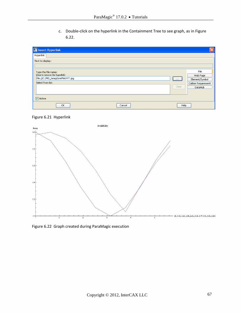
ParaMagic® 17.0.2 Tutorials
Copyright © 2012, InterCAX LLC 67
c. Double-click on the hyperlink in the Containment Tree to see graph, as in Figure
6.22.
Figure 6.21 Hyperlink
Figure 6.22 Graph created during ParaMagic execution

ParaMagic® 17.0.2 Tutorials
Copyright © 2012, InterCAX LLC 68
7 SYSML PARAMETRICS TUTORIAL - HOMEHEATING
Note: ParaMagic Lite does not have the ability to call MATLAB functions and scripts. The
HomeHeating model will not be executable without upgrading to the full ParaMagic feature set. Standard
ParaMagic users must set Mathematica as the core solver to access all program features.
7.1 Objective
Create a SysML project incorporating a Simulink simulation model of a home heating system and
a MATLAB function that predicts outside temperature. The Simulink model, a minor modification of a
standard demonstration model from MathWorks, is shown in Figure 7.1. Input 1 is the outside
temperature, which varies periodically through the day and through the year. Outputs 1, 2 and 3 are the
cumulative cost, indoor temperature, and outdoor temperature as a function of time. The objective is to
estimate the cost per day of heating the home.
Figure 7.1 Outline of Objective
What the User Will Learn
Connect to MATLAB functions and scripts through SysML constraint blocks
Connect to Simulink models through SysML constraint blocks

ParaMagic® 17.0.2 Tutorials
Copyright © 2012, InterCAX LLC 69
A large body of simulation models have been developed and validated using MATLAB and
Simulink (The MathWorks, Inc.). Being able to incorporate these existing models into larger SysML
models can greatly accelerate system development. ParaMagic allows Simulink/MATLAB models to be
treated as “black box” constraint blocks within MagicDraw parametric models. ParaMagic does not
convert SysML models into Simulink models or the reverse.
We assume in this tutorial that the reader is familiar with MATLAB and Simulink and focus
completely on the steps necessary to interface existing MATLAB/Simulink elements to SysML
parametric diagrams. For further help, see the ParaMagic Users Guide and the user documentation for
MagicDraw and MATLAB.
7.2 Step-by Step Tutorial
Step I Create Project
1. Create new project
a. Name = HomeHeating
2. Create a package within the project
a. RC (Right-click) on Data folder in Containment tree (left column)
b. Choose New Element→Package
c. Enter Name = HomeHeating
Step II Create Infrastructure
3. Install ParaMagic Profile module.
Step III Create Structural Model
4. Create elements in model
a. Inside the HomeHeating package, create blocks HomeHeatingSystem, Home and
Outdoors.
b. Create a block definition diagram, Name = HomeHeating, and drag the blocks into the
diagram. See Figure 7.2. Note that we use a Directed Composition connector to link
HomeHeatingSystem to Home but reference the Outdoors block with a Directed
Aggregation arrow.
c. Create the Value Properties shown in Figure 7.2. All are Real with a multiplicity of 1.
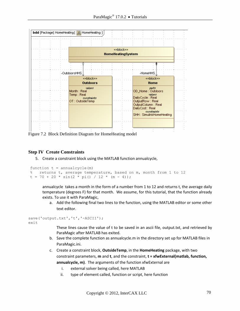
ParaMagic® 17.0.2 Tutorials
Copyright © 2012, InterCAX LLC 70
Step IV Create Constraints
5. Create a constraint block using the MATLAB function annualcycle,
function t = annualcycle(m) % returns t, average temperature, based on m, month from 1 to 12 t = 70 + 20 * sin(2 * pi() / 12 * (m - 4));
annualcycle takes a month in the form of a number from 1 to 12 and returns t, the average daily temperature (degrees F) for that month. We assume, for this tutorial, that the function already exists. To use it with ParaMagic,
a. Add the following final two lines to the function, using the MATLAB editor or some other
text editor.
save('output.txt','t','-ASCII'); exit
These lines cause the value of t to be saved in an ascii file, output.txt, and retrieved by ParaMagic after MATLAB has exited.
b. Save the complete function as annualcycle.m in the directory set up for MATLAB files in
ParaMagic.ini.
c. Create a constraint block, OutsideTemp, in the HomeHeating package, with two
constraint parameters, m and t, and the constraint, t = xfwExternal(matlab, function,
annualcycle, m). The arguments of the function xfwExternal are
i. external solver being called, here MATLAB
ii. type of element called, function or script, here function
Figure 7.2 Block Definition Diagram for HomeHeating model
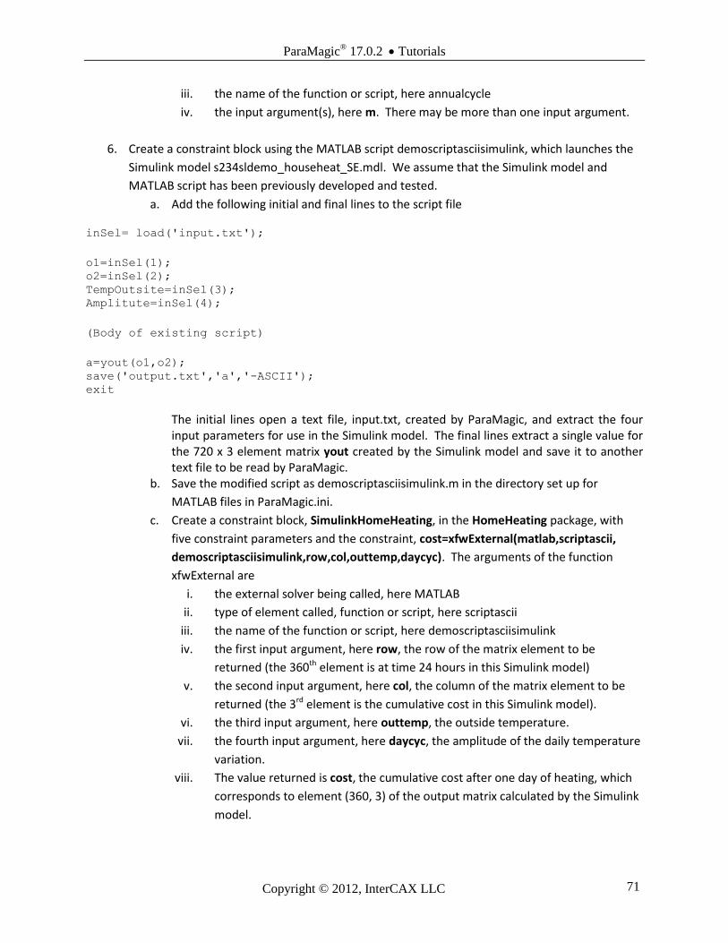
ParaMagic® 17.0.2 Tutorials
Copyright © 2012, InterCAX LLC 71
iii. the name of the function or script, here annualcycle
iv. the input argument(s), here m. There may be more than one input argument.
6. Create a constraint block using the MATLAB script demoscriptasciisimulink, which launches the
Simulink model s234sldemo_househeat_SE.mdl. We assume that the Simulink model and
MATLAB script has been previously developed and tested.
a. Add the following initial and final lines to the script file
inSel= load('input.txt');
o1=inSel(1); o2=inSel(2); TempOutsite=inSel(3); Amplitute=inSel(4);
(Body of existing script)
a=yout(o1,o2); save('output.txt','a','-ASCII'); exit
The initial lines open a text file, input.txt, created by ParaMagic, and extract the four input parameters for use in the Simulink model. The final lines extract a single value for the 720 x 3 element matrix yout created by the Simulink model and save it to another text file to be read by ParaMagic.
b. Save the modified script as demoscriptasciisimulink.m in the directory set up for
MATLAB files in ParaMagic.ini.
c. Create a constraint block, SimulinkHomeHeating, in the HomeHeating package, with
five constraint parameters and the constraint, cost=xfwExternal(matlab,scriptascii,
demoscriptasciisimulink,row,col,outtemp,daycyc). The arguments of the function
xfwExternal are
i. the external solver being called, here MATLAB
ii. type of element called, function or script, here scriptascii
iii. the name of the function or script, here demoscriptasciisimulink
iv. the first input argument, here row, the row of the matrix element to be
returned (the 360th element is at time 24 hours in this Simulink model)
v. the second input argument, here col, the column of the matrix element to be
returned (the 3rd element is the cumulative cost in this Simulink model).
vi. the third input argument, here outtemp, the outside temperature.
vii. the fourth input argument, here daycyc, the amplitude of the daily temperature
variation.
viii. The value returned is cost, the cumulative cost after one day of heating, which
corresponds to element (360, 3) of the output matrix calculated by the Simulink
model.
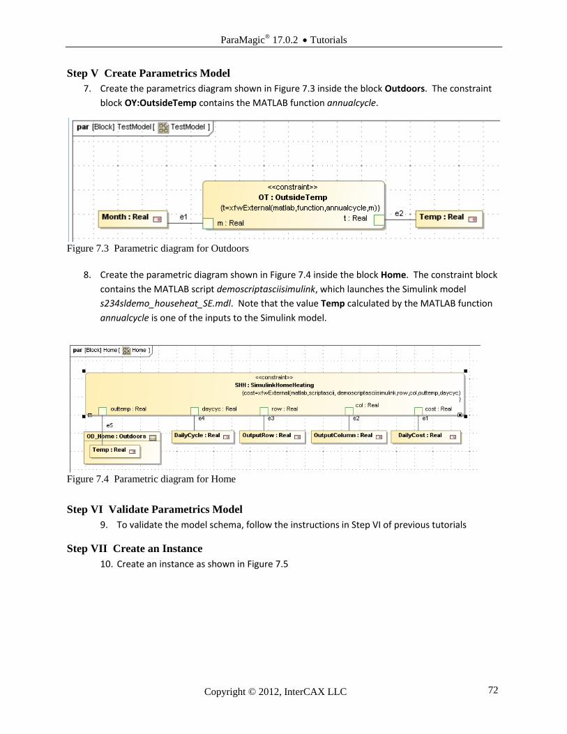
ParaMagic® 17.0.2 Tutorials
Copyright © 2012, InterCAX LLC 72
Step V Create Parametrics Model
7. Create the parametrics diagram shown in Figure 7.3 inside the block Outdoors. The constraint
block OY:OutsideTemp contains the MATLAB function annualcycle.
8. Create the parametric diagram shown in Figure 7.4 inside the block Home. The constraint block
contains the MATLAB script demoscriptasciisimulink, which launches the Simulink model
s234sldemo_househeat_SE.mdl. Note that the value Temp calculated by the MATLAB function
annualcycle is one of the inputs to the Simulink model.
Step VI Validate Parametrics Model
9. To validate the model schema, follow the instructions in Step VI of previous tutorials
Step VII Create an Instance
10. Create an instance as shown in Figure 7.5
Figure 7.3 Parametric diagram for Outdoors
Figure 7.4 Parametric diagram for Home

ParaMagic® 17.0.2 Tutorials
Copyright © 2012, InterCAX LLC 73
Figure 7.5 Instance of HomeHeatingSystem
a. Point the Part Property OD_Home inside Home03 to the instance OD03:Outdoors.
Note that this assignment is not made automatically in creating the linkages, as in
previous examples.
i. Open the Instance Specification for Home03 (Figure 7.6)
ii. Select Slots
iii. Click on OD_Home:Outdoors
iv. Click Create Value button
Figure 7.6 Instance Specification for Home03

ParaMagic® 17.0.2 Tutorials
Copyright © 2012, InterCAX LLC 74
v. Select OD03:HomeHeating:Outdoors in the Select Elements window (see Figure
7.7)
vi. Click Add, OK, and Close
Figure 7.7 Select Elements to link OD03 to OD_Home
b. Create the links and populate the slots as shown in previous tutorials. The givens are
i. Month = 1 (January)
ii. DailyCycle = 10 (temperature varies +/- 10 daily)
iii. Row = 360 (one day as Simulink model timescale is set)
iv. Col = 3 (cumulative cost as Simulink model output array is configured)
c. Assign causalities to slots using the Add default causalities utility. Change causality of
DailyCost to target.

ParaMagic® 17.0.2 Tutorials
Copyright © 2012, InterCAX LLC 75
Step VIII Solve the Instance
11. Open the Browser (Figure 7.8) and click Solve.
Figure 7.8 Browser before solution
a. During ParaMagic execution, MATLAB will launch and several figures will appear
briefly on your screen, including the Simulink model diagram from Figure 7.1 and
the PlotResults graph shown in Figure 7.9. The PlotResults window shows the
cumulative cost in the upper window over a two day period. The lower window
shows the outdoor temperature (violet) and the indoor temperature (yellow) on the
same time scale. The target indoor temperature is a constant, 70 F, set inside the
Simulink model (although the model could be modified to treat this as an input from
SysML, as well), but the actual indoor temperature varies as the thermostat cycles
on and off.
The appearance of these figures is set in the Simulink model, not in the SysML
model or in the MATLAB script. These windows will disappear when the simulation
is complete and MATLAB exits.
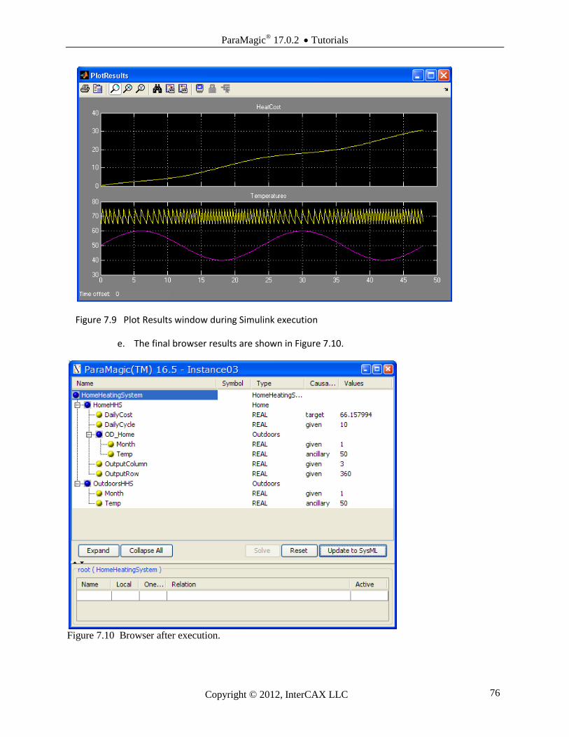
ParaMagic® 17.0.2 Tutorials
Copyright © 2012, InterCAX LLC 76
Figure 7.9 Plot Results window during Simulink execution
e. The final browser results are shown in Figure 7.10.
Figure 7.10 Browser after execution.
ParaMagic® 17.0.2 Tutorials
Copyright © 2012, InterCAX LLC 77
8 SYSML PARAMETRICS TUTORIAL – LITTLEEYE TRADE STUDY
8.1 Objective
This tutorial is a continuation of the LittleEye exercise in Section 4. Once a parametric model is
built and validated, users frequently want to explore variations in the initial parameter set. This can be
called a trade study, sensitivity analysis, or design of experiments and is helpful in identifying key inputs,
assessing risk and optimizing results.
ParaMagic uses the Excel Connection feature to set up the different initial parameter sets or
“scenarios” as rows in a spreadsheet. Parameter sets are automatically read, the model is repeatedly
executed and output values written back to the spreadsheet. Using the LittleEye model, we will run a
multi-variable trade study, to determine the sensitivity of the result to the number of planes, crews and
fuel loads available.
What the User Will Learn
Running a ParaMagic trade study
8.2 Step-by-Step Tutorial
Step VII Set-up a Trade Study
Start with the LittleEye model created in Section
4. The trade study uses the same ExcelConnection
interface that was described in the earlier Orbital tutorial.
The only difference is that, instead of reading in a single
set of values from the spreadsheet, processing them
using the parametric solver, and writing the results back
to the spreadsheet, the Trades Studies feature runs
multiple value sets in an automated batch mode process.
1. Create an MS Excel spreadsheet for the
trade study, as in Table 8.1. The trade
study will vary two parameters, Number of
Planes and Number of Crews, and calculate
a single output value, Miles Scanned Per 24
Hours. Each row is a single trial or
scenario. The trade study will start with
the first trial designated in the Excel
interface and work down one row at a
time. In this trade, we have 20 trials, a
combinatorial explosion of 3,4,5,6 and 7
planes and 4, 5, 6 and 7 crews. We save
the spreadsheet as LE_Trade.xlsx.
2. Set up the Excel linkages for Read and
Write as in the Orbital tutorial.
a. RC LittleEyeInstance01 and select ParaMagic→ Excel→ Setup
Number of Planes
Number of Crews
Miles Scanned Per 24 Hours
3 4 4 4 5 4 6 4 7 4 3 5 4 5 5 5 6 5 7 5 3 6 4 6 5 6 6 6 7 6 3 7 4 7 5 7 6 7 7 7 Table 8.1 LE_Trade.xlsx

ParaMagic® 17.0.2 Tutorials
Copyright © 2012, InterCAX LLC 78
b. Select NumberPlanes
i. Enter LE_Trade.xlsx under Workbook
ii. Click Refresh
iii. Select Sheet1 under Worksheet.
iv. Under Cell Range, enter A2, the cell containing the first trial value for this
parameter. Do not enter a cell range; the number of trials will be specified
later.
v. Under Access Mode, select Read (see Figure 8.1)
c. Repeat for NumberCrews, with Cell Range = B2, Access Mode = Read
d. Repeat for MilesScannedPer24Hours, Cell Range = C2, Access Mode = Write.
e. Click OK to close Excel Setup window.
3. Set number of trade study scenarios to run.
a. Right-click on LittleEyeInstance01 and select ParaMagic→ Trade Study→ Setup.
b. As shown in Figure 8.2, enter the number of scenarios (20 in this example) and click OK.
Figure 8.1 Excel Setup window for trade study
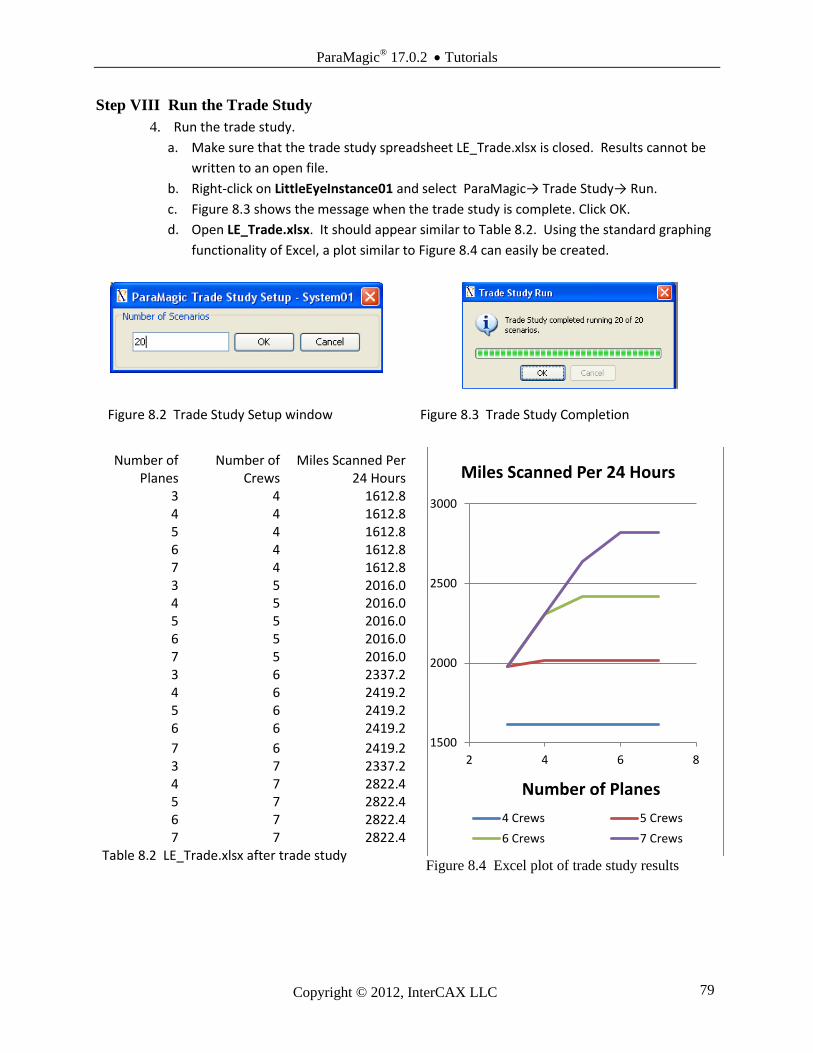
ParaMagic® 17.0.2 Tutorials
Copyright © 2012, InterCAX LLC 79
Step VIII Run the Trade Study
4. Run the trade study.
a. Make sure that the trade study spreadsheet LE_Trade.xlsx is closed. Results cannot be
written to an open file.
b. Right-click on LittleEyeInstance01 and select ParaMagic→ Trade Study→ Run.
c. Figure 8.3 shows the message when the trade study is complete. Click OK.
d. Open LE_Trade.xlsx. It should appear similar to Table 8.2. Using the standard graphing
functionality of Excel, a plot similar to Figure 8.4 can easily be created.
Figure 8.2 Trade Study Setup window Figure 8.3 Trade Study Completion
Figure 8.4 Excel plot of trade study results
1500
2000
2500
3000
2 4 6 8
Number of Planes
Miles Scanned Per 24 Hours
4 Crews 5 Crews
6 Crews 7 Crews
Number of Planes
Number of Crews
Miles Scanned Per 24 Hours
3 4 1612.8 4 4 1612.8 5 4 1612.8 6 4 1612.8 7 4 1612.8 3 5 2016.0 4 5 2016.0 5 5 2016.0 6 5 2016.0 7 5 2016.0 3 6 2337.2 4 6 2419.2 5 6 2419.2 6 6 2419.2
7 6 2419.2 3 7 2337.2 4 7 2822.4 5 7 2822.4 6 7 2822.4 7 7 2822.4
Table 8.2 LE_Trade.xlsx after trade study
ParaMagic® 17.0.2 Tutorials
Copyright © 2012, InterCAX LLC 80
9 SYSML PARAMETRICS TUTORIAL - ELECTRONICS
Note: ParaMagic Lite does not have the ability to calculate with complex aggregates. The Electronics
model will not be executable without upgrading to the full ParaMagic feature set. Standard ParaMagic
users must set Mathematica as the core solver to access all program features.
9.1 Objective
Create a SysML project describing a computer center that will be built in a variety of standard
configurations. Each configuration of the center will consist of one or more independent computer cells,
each composed of one or more server arrays, disk arrays, and other components. Each configuration can
also be viewed as consisting of one or more electronics racks, each of which contains one or more
electronic boxes, which might be a server array, a disk array, or some other component belonging to one
of the cells.
Each of the standard configurations has a specific set of requirements that it must meet in terms
of the number of cells and total computing capacity, e.g. server calculating speed, disk storage. In
addition, each rack has a set of requirements that cannot be exceeded, including physical space, electrical
power, cooling capacity, etc. Our objective is to create a SysML model that requires the minimum
modeling effort, yet describes the full range of standard configurations and can test parametrically
whether each configuration meets its requirements. Creating and modifying configurations should be
simple and intuitive, so alternative designs can be evaluated. For simplicity, this tutorial only considers a
few types of components and requirements.
Ordinarily, this type of problem is handled with a spreadsheet, which can grow quite complex.
Handling these same calculations inside the SysML model parametrically has several advantages,
There is a single model, not a model and separate spreadsheet which must be synchronized,
There is a clear distinction between the abstract model (the schema) and the concrete
configurations (instances) in SysML,
The calculations are not hidden inside spreadsheet cells, but readily seen, modified and
documented in the SysML model itself.
What the User Will Learn
Using complex aggregates
Using generalization/specialization
Working with requirements
Complex aggregates involve parameters shared by part properties with a multiplicity greater than
one. For example, if an assembly contains four equivalent parts, the weights of the four parts comprise a
complex aggregate of four values. This contrasts with the earlier concept of a primitive aggregate, a
single parameter containing multiple values. ParaMagic allows the user to sum, average, find a
maximum, or find a minimum of a complex aggregate, similar to the fashion in which primitive
aggregates are used in the Orbital example. The great value of complex aggregates is that parametric
relationships can be defined at the schema level without specifying the number of parts that will be used
in a specific instance.
Another useful feature of SysML is inheritance, or the ability to create generalized and
specialized forms of a system object. This helps when we want to group diverse objects in one set of
parametric calculations, but use each object’s unique properties in other calculations.
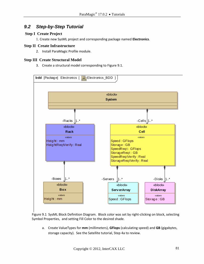
ParaMagic® 17.0.2 Tutorials
Copyright © 2012, InterCAX LLC 81
9.2 Step-by-Step Tutorial
Step I Create Project
1. Create new SysML project and corresponding package named Electronics.
Step II Create Infrastructure
2. Install ParaMagic Profile module.
Step III Create Structural Model
3. Create a structural model corresponding to Figure 9.1.
Figure 9.1 SysML Block Definition Diagram. Block color was set by right-clicking on block, selecting Symbol Properties, and setting Fill Color to the desired shade.
a. Create ValueTypes for mm (millimeters), GFlops (calculating speed) and GB (gigabytes,
storage capacity). See the Satellite tutorial, Step 4a to review.
Electronics_BDDElectronics[Packag e] bdd [ ]
«block»
System
values
Speed : GFlops
Storag e : GB
SpeedReq t : GFlops
Storag eReq t : GB
SpeedReq tVerify : Real
Storag eReq tVerify : Real
«block»
Cell
values
Heig ht : mm
«block»
Boxvalues
Heig ht : mm
Heig htReq tVerify : Real
«block»
Rack
values
Heig ht : mm
«block»
Box values
Speed : GFlops
«block»
Serv erArray
values
Storag e : GB
«block»
DiskArray
values
Speed : GFlops
«block»
Serv erArray values
Storag e : GB
«block»
DiskArray
-Boxes 1..* -Servers 1..* -Disks 1..*
-Cells 1..*-Racks 1..*
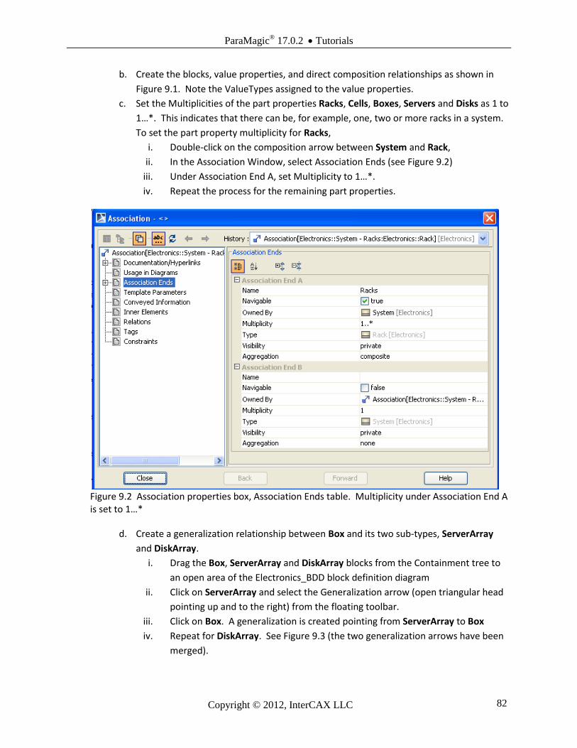
ParaMagic® 17.0.2 Tutorials
Copyright © 2012, InterCAX LLC 82
b. Create the blocks, value properties, and direct composition relationships as shown in
Figure 9.1. Note the ValueTypes assigned to the value properties.
c. Set the Multiplicities of the part properties Racks, Cells, Boxes, Servers and Disks as 1 to
1…*. This indicates that there can be, for example, one, two or more racks in a system.
To set the part property multiplicity for Racks,
i. Double-click on the composition arrow between System and Rack,
ii. In the Association Window, select Association Ends (see Figure 9.2)
iii. Under Association End A, set Multiplicity to 1…*.
iv. Repeat the process for the remaining part properties.
Figure 9.2 Association properties box, Association Ends table. Multiplicity under Association End A is set to 1…*
d. Create a generalization relationship between Box and its two sub-types, ServerArray
and DiskArray.
i. Drag the Box, ServerArray and DiskArray blocks from the Containment tree to
an open area of the Electronics_BDD block definition diagram
ii. Click on ServerArray and select the Generalization arrow (open triangular head
pointing up and to the right) from the floating toolbar.
iii. Click on Box. A generalization is created pointing from ServerArray to Box
iv. Repeat for DiskArray. See Figure 9.3 (the two generalization arrows have been
merged).
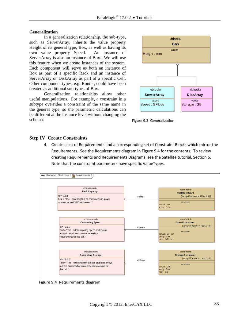
ParaMagic® 17.0.2 Tutorials
Copyright © 2012, InterCAX LLC 83
Generalization
In a generalization relationship, the sub-type,
such as ServerArray, inherits the value property
Height of its general type, Box, as well as having its
own value property Speed. An instance of
ServerArray is also an instance of Box. We will use
this feature when we create instances of the system.
Each component will serve as both an instance of
Box as part of a specific Rack and an instance of
ServerArray or DiskArray as part of a specific Cell.
Other component types, e.g. Router, could have been
created as additional sub-types of Box.
Generalization relationships allow other
useful manipulations. For example, a constraint in a
subtype overrides a constraint of the same name in
the general type, so the parametric calculations can
be different at the instance level without changing the
schema.
Step IV Create Constraints
4. Create a set of Requirements and a corresponding set of Constraint Blocks which mirror the
Requirements. See the Requirements diagram in Figure 9.4 for the contents. To review
creating Requirements and Requirements Diagrams, see the Satellite tutorial, Section 6.
Note that the constraint parameters have specific ValueTypes.
Figure 9.4 Requirements diagram
Req uirementsElectronics[Packag e] req [ ]
Id = "1.0.1"
Text = "The total height of all components in a rack
must not exceed 1000 millimeters. "
«requirement»
Rack Capacity
Id = "2.0.2"
Text = "The total longterm storage of all disk arrays
in a cell must meet or exceed the requirements for
that cell. "
«requirement»
Computing Storage
Id = "2.0.1"
Text = "The total computing speed of all server
arrays in a cell must meet or exceed the
requirements for that cell. "
«requirement»
Computing Speed
paramet ers
actual : GB
verify : Real
req t : GB
«constraint»
StorageConstraint
{verify=if(actual>= reqt, 1, 0)}
paramet ers
actual : GFlops
verify : Real
req t : GFlops
«constraint»
SpeedConstraint
{verify=if(actual>= reqt, 1, 0)}
paramet ers
actual : mm
verify : Real
«constraint»
RackConstraint
{verify=if(actual<= 1000, 1, 0)}«refine»
«refine»
«refine»
Figure 9.3 Generalization
Electronics_BDDElectronics[Packag e] bdd [ ]
«block»
System
values
Speed : GFlops
Storag e : GB
SpeedReq t : GFlops
Storag eReq t : GB
SpeedReq tVerify : Real
Storag eReq tVerify : Real
«block»
Cell
values
Heig ht : mm
«block»
Boxvalues
Heig ht : mm
Heig htReq tVerify : Real
«block»
Rack
values
Heig ht : mm
«block»
Box values
Speed : GFlops
«block»
Serv erArray
values
Storag e : GB
«block»
DiskArray
values
Speed : GFlops
«block»
Serv erArray values
Storag e : GB
«block»
DiskArray
-Boxes 1..* -Servers 1..* -Disks 1..*
-Cells 1..*-Racks 1..*
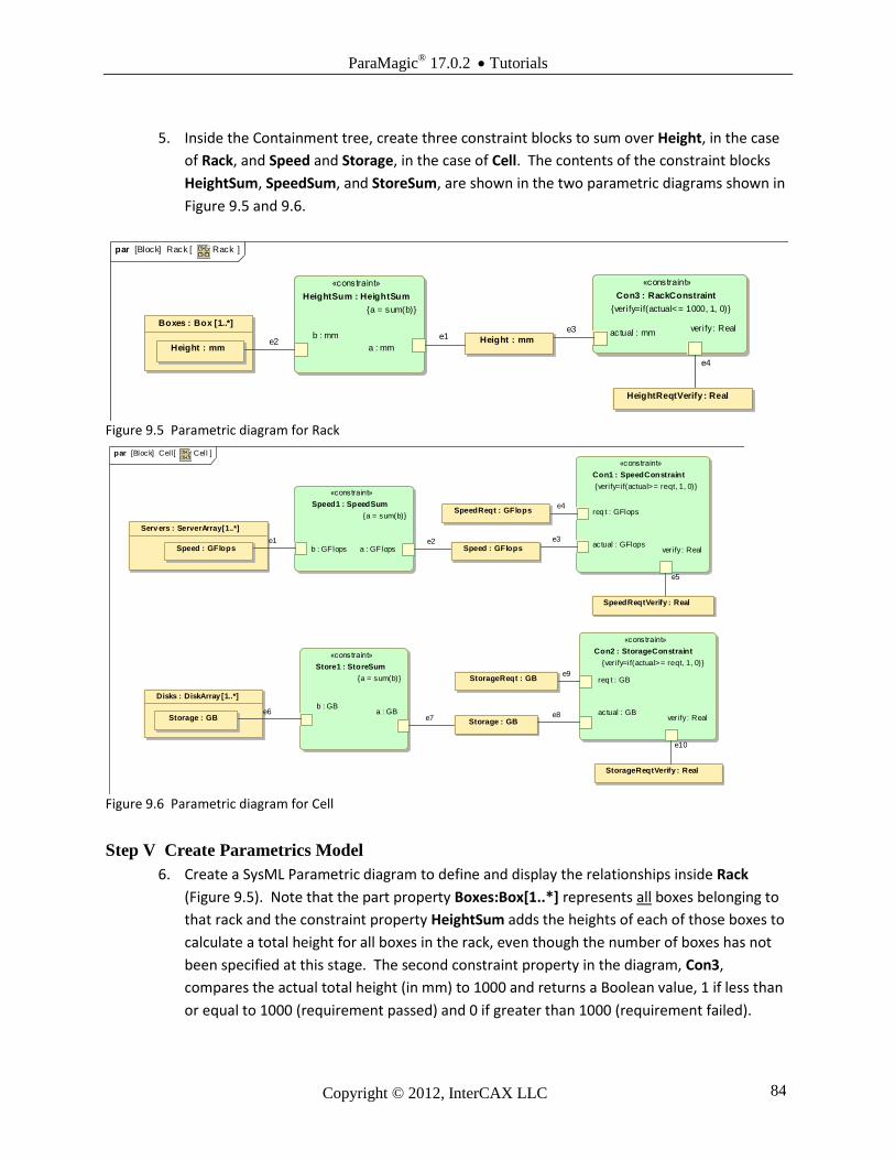
ParaMagic® 17.0.2 Tutorials
Copyright © 2012, InterCAX LLC 84
5. Inside the Containment tree, create three constraint blocks to sum over Height, in the case
of Rack, and Speed and Storage, in the case of Cell. The contents of the constraint blocks
HeightSum, SpeedSum, and StoreSum, are shown in the two parametric diagrams shown in
Figure 9.5 and 9.6.
Figure 9.5 Parametric diagram for Rack
Figure 9.6 Parametric diagram for Cell
Step V Create Parametrics Model
6. Create a SysML Parametric diagram to define and display the relationships inside Rack
(Figure 9.5). Note that the part property Boxes:Box[1..*] represents all boxes belonging to
that rack and the constraint property HeightSum adds the heights of each of those boxes to
calculate a total height for all boxes in the rack, even though the number of boxes has not
been specified at this stage. The second constraint property in the diagram, Con3,
compares the actual total height (in mm) to 1000 and returns a Boolean value, 1 if less than
or equal to 1000 (requirement passed) and 0 if greater than 1000 (requirement failed).
[Block] Rack Rackpar [ ]
«constraint»
Con3 : RackConstraint
{verify=if(actual<= 1000, 1, 0)}
actual : mmverify : Real
HeightReqtVerify : Real
«constraint»
HeightSum : HeightSum
{a = sum(b)}
a : mm
b : mm
Height : mm
Boxes : Box [1..*]
Height : mme2
e3e1
e4
[Block] par Cell Cell[ ]
Speed : GFlops
Serv ers : ServerArray [1..*]
«constraint»
Con2 : StorageConstraint
{verify=if(actual>= reqt, 1, 0)}
actual : GB
req t : GB
verify : Real
«constraint»
Con1 : SpeedConstraint
{verify=if(actual>= reqt, 1, 0)}
actual : GFlops
req t : GFlops
verify : Real
StorageReqtVerify : Real
SpeedReqtVerify : Real
«constraint»
Speed1 : SpeedSum
{a = sum(b)}
a : GFlopsb : GFlops
Storage : GB
Disks : DiskArray [1..*]
«constraint»
Store1 : StoreSum
{a = sum(b)}
a : GBb : GB
SpeedReqt : GFlops
StorageReqt : GB
Speed : GFlops
Storage : GB
e1
e6e7 e8
e3e2
e4
e10
e5
e9
ParaMagic® 17.0.2 Tutorials
Copyright © 2012, InterCAX LLC 85
7. Create a second SysML Parametric diagram to define and display the calculation of the
requirements verification relationships inside Cell (Figure 9.6). This appears like a doubling
of the Height requirement checking, with one branch for calculating speed of the Servers
and another for the storage capacity of the Disks. Note that the Speed and Storage
Requirements are left as variables, where the Height Requirement was “hard-coded” as
1000 in the constraint. In this project, each configuration (instance) of the system will have
different speed and storage needs, while racks are of a standard size.
Step VI Validate Parametrics Model
8. To validate the model schema, RC on System in the Containment tree and select
ParaMagic→Validate
Discussion - Schema and Instance
At this stage, we have created a rather simple schema which may be applied to multiple instances
of arbitrary complexity. The algorithms we use to calculate system performance and resource needs are
created once in an easily understood graphical format (parametric diagram), and re-used wherever the
block holding that parametric diagram occurs. Compare this with a typical spreadsheet, where the
distinction between schema and instance is not made. Each formula is buried in multiple cells, all of
which must be updated when the model is changed. While spreadsheets excel at the organization and
presentation of tabular data, they have their limits as system modeling tools.
Step VII Create an Instance
9. Create an instance library containing an instance block for each of the standard components
to be used in building real system configurations. These instances can be used in each of
the configurations we build.
a. RC Electronics and create a new Package = InstanceLibrary
b. RC InstanceLibrary and create a new Instance Specification with Name =
A501_Server and Classifier = ServerArray
c. Assign values of 200 (mm) and 15 (GFlops) to the Height and Speed slots in
A501_Server.
d. RC InstanceLibrary and create a new Instance Specification with Name = J30_Disk
and Classifier = DiskArray
e. Activate the Height and Speed slots in J30_Disk and assign values of 300 (mm) and 5
(GB).
f. RC InstanceLibrary and select ParaMagic→Util→ Assign Default Causality.
10. Create an instance of a system configuration comprised of one computer cell spread over
two racks. See Figure 9.7.
a. RC Electronics and create a new Package = Instance01
b. In Instance01, create one instance of System (System01), two instances of Rack
(Rack1 and Rack2), and one instance of Cell (Cell1).
c. In Instance01, create a block definition diagram Instance01.
d. Drag System01, Cell1, Rack1 and Rack2 into the diagram.

ParaMagic® 17.0.2 Tutorials
Copyright © 2012, InterCAX LLC 86
e. Drag A501_Server into the diagram 3 times. This creates 3 symbols of the same
instance block, not 3 blocks.
f. Drag J30_Disk into the diagram 3 times.
g. Create the links as shown in Figure 9.7. Note that each component instance is
linked to one rack (where it is physically located) and one cell (where it is
electronically part of a specific computer system).
Figure 9.7 Instance01 diagram containing one Cell spread over two Racks
h. Activate the slots in the rack and cell instances. In Cell1, SpeedReqt = 50 and
StorageReqt = 10. Other values are initially unknowns.
i. Apply Assign Default Causality to Instance01. Change causality of the …Verify slots
to target.
Discussion – Instance Libraries
There are alternate ways to build instances from instance libraries, which may provide the same
answers but each with different strengths and weaknesses.
Instance01 Instance01[Packag e] bdd [ ]
Cells = Cell1
Racks = Rack1 , Rack2
«block»
System01 : System
Disks = J30_Disk ,
J30_Disk, J30_Disk
Servers = A501_Server ,
A501_Server, A501_Server
Speed = ""
SpeedReqt = "50"
SpeedReqtVerify = ""
Storage = ""
StorageReqt = "10"
StorageReqtVerify = ""
«block»
Cell1 : Cell
Height = "200"
Speed = "15"
«block»
A501_Serv er : Serv erArray
Height = "200"
Speed = "15"
«block»
A501_Serv er : Serv erArray
Height = "200"
Speed = "15"
«block»
A501_Serv er : Serv erArray
Boxes = A501_Server ,
A501_Server, J30_Disk
Height = ""
HeightReqtVerify = ""
«block»
Rack1 : Rack
Boxes = A501_Server ,
J30_Disk, J30_Disk
Height = ""
HeightReqtVerify = ""
«block»
Rack2 : Rack
Height = "300"
Storage = "5"
«block»
J30_Disk : DiskArray
Height = "300"
Storage = "5"
«block»
J30_Disk : DiskArray
Height = "300"
Storage = "5"
«block»
J30_Disk : DiskArray

ParaMagic® 17.0.2 Tutorials
Copyright © 2012, InterCAX LLC 87
In the approach shown above, a single instance block of each type appears multiple times in the
diagram, but each diagram symbol refers back to the same instance. A change in a slot value for
the instance block will appear in all of the diagram symbols for that component.
Alternately, we could cut-and-paste multiple copies of the component in InstanceLibrary into
Instance01, then drag those copies into the instance diagram. In this case, each instance of the
component is independent and each slot value can be varied independently. This is a much better
approach when the instance block contains an unknown calculated during parametric execution,
because each instance can hold a different calculated value for this slot.
Alternately, we could drag a single instance block into the diagram and create multiple links to it.
For example, the A501_Server instance block would be the destination of two links from Rack1,
three from Cell1 and one from Rack2. While the resulting diagram might be somewhat smaller,
it mignt also be more difficult to understand.
Step VIII Solve the Instance
11. Run the parametric solver
a. RC the Instance_01 package.
b. Select ParaMagic→Browse.
Figure 9.8 ParaMagic Browser for Instance_01, before solution, partially expanded
c. Press “Solve”. The results in Figure 9.9 show 1 (Pass) for HeightReqtVerify for both
racks and for StorageReqtVerify for Cell1. SpeedReqtVerify for Cell1 is 0 (Fail)
because the cumulative calculating speed of all servers in the cell is 45 GFlops, less
than the requirement of 50.

ParaMagic® 17.0.2 Tutorials
Copyright © 2012, InterCAX LLC 88
Figure 9.9 ParaMagic Browser for Instance_01, after solution
Step VII Create an Instance (Second Configuration)
12. Create a new instance of a system configuration comprised of two computer cells spread
over three racks. See Figure 9.10. Repeat process in Step 10.
Step VIII Solve the Instance (Second Configuration)
13. Run the parametric solver. See Figure 9.11 for results. Note that no changes had to be made
to the parametric diagram or any other part of the schema to run the new parametric model
calculations.
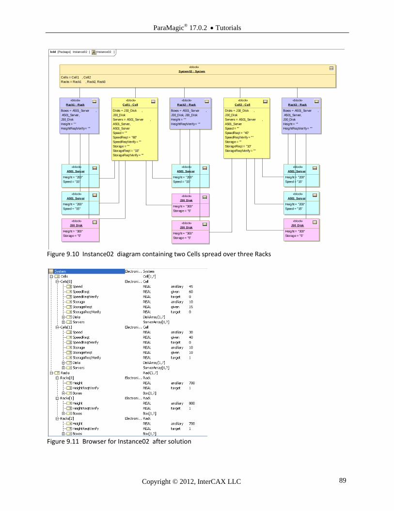
ParaMagic® 17.0.2 Tutorials
Copyright © 2012, InterCAX LLC 89
Figure 9.10 Instance02 diagram containing two Cells spread over three Racks
Figure 9.11 Browser for Instance02 after solution
Instance02 Instance02[Packag e] bdd [ ]
Cells = Cell1 , Cell2
Racks = Rack1 , Rack2, Rack3
«block»
System02 : System
Disks = J30_Disk ,
J30_Disk
Servers = A501_Server ,
A501_Server,
A501_Server
Speed = ""
SpeedReqt = "60"
SpeedReqtVerify = ""
Storage = ""
StorageReqt = "15"
StorageReqtVerify = ""
«block»
Cell1 : Cell
Disks = J30_Disk ,
J30_Disk
Servers = A501_Server ,
A501_Server
Speed = ""
SpeedReqt = "40"
SpeedReqtVerify = ""
Storage = ""
StorageReqt = "10"
StorageReqtVerify = ""
«block»
Cell2 : Cell
Boxes = A501_Server ,
J30_Disk, J30_Disk
Height = ""
HeightReqtVerify = ""
«block»
Rack2 : Rack
Boxes = A501_Server ,
A501_Server,
J30_Disk
Height = ""
HeightReqtVerify = ""
«block»
Rack3 : Rack
Boxes = A501_Server ,
A501_Server,
J30_Disk
Height = ""
HeightReqtVerify = ""
«block»
Rack1 : Rack
Height = "200"
Speed = "15"
«block»
A501_Serv er
Height = "300"
Storage = "5"
«block»
J30_Disk
Height = "200"
Speed = "15"
«block»
A501_Serv er
Height = "200"
Speed = "15"
«block»
A501_Serv er
Height = "300"
Storage = "5"
«block»
J30_Disk
Height = "300"
Storage = "5"
«block»
J30_Disk
Height = "300"
Storage = "5"
«block»
J30_Disk
Height = "200"
Speed = "15"
«block»
A501_Serv er
Height = "200"
Speed = "15"
«block»
A501_Serv er