Parallel Techniques for Physically-Based Simulation on Multi-Core ProcessorArchitectures

Bernhard Thomaszewski a,∗ Simon Pabst a Wolfgang Blochinger b

aWSI/GRIS, Universitat Tubingen, GermanybSymbolic Computation Group, Universitat Tubingen, Germany

Abstract

As multi-core processor systems become more and more widespread, the demand for efficient parallel algorithms also propagatesinto the field of computer graphics. This is especially true for physically-based simulation, which is notorious for expensivenumerical methods. In this work, we explore possibilities for accelerating physically-based simulation algorithms on multi-corearchitectures. Two components of physically-based simulation represent a great potential for bottlenecks in parallelisation: implicittime integration and collision handling. From the parallelisation point of view these two components are substantially different.Implicit time integration can be treated efficiently using static problem decomposition. The linear system arising in this contextis solved using a data-parallel preconditioned conjugate gradient algorithm. The collision handling stage, however, requires adifferent approach, due to its dynamic structure. This stage is handled using multi-threaded programming with fully dynamic taskdecomposition. In particular, we propose a new task splitting approach based on a reasonable estimation of work, which analysesprevious simulation steps. Altogether, the combination of different parallelisation techniques leads to a concise and yet versatileframework for highly efficient physical simulation.

Key words:

Physically-Based Simulation, Parallel Collision Detection, Parallel Conjugate Gradients, Multi-Core Processors

1. Introduction

Physically-based simulation is an important componentof many applications in current research areas of computergraphics. The most prominent examples are fluid, soft body,and cloth simulation. All of these applications utilise com-putationally intensive methods and runtimes for realisticscenarios are often excessive. Obviously, increasing the re-alism of the simulation by using more accurate methods,like finite elements, further aggravates the problem. In thispaper we investigate on parallel techniques for improvingthe performance of physically-based simulation codes onmulti-core architectures.

Generally, most of the computation time is spent ontwo stages, time integration and collision handling. Inthe following, we will therefore consider these two major

∗ Corresponding author.Email address: b.thomaszewski@gris.uni-tuebingen.de

(Bernhard Thomaszewski).URL: www.gris.uni-tuebingen.de/∼thomasze (Bernhard

Thomaszewski).

bottlenecks, which are present in almost every physically-based simulation. Although we focus on cloth simulationin this work, the techniques proposed herein transfer tomany other applications, like e.g. thin-shell and three-dimensional soft body simulation.

1.1. Implicit time integration

Often, the physical model at the centre of a specific sim-ulator gives rise to stiff differential equations with respectto time. For stability reasons implicit schemes are widelyaccepted as the method of choice for numerical time inte-gration (cf. [1]). Implicit schemes require the solution of a(non-)linear system of equations at each time step. As aresult of the spatial discretisation, the matrix of this sys-tem is usually very sparse. There are essentially two alter-natives for the numerical solution of the system. One is touse an iterative method such as the popular conjugate gra-dients (cg) algorithm [2]. Another is to use direct sparsesolvers, which are usually based on fill-reducing reorderingand factorisation. The cg-method is favoured in computer

Preprint submitted to Computers and Graphics 11 April 2008

graphics as it offers much simpler user interaction, allevi-ates the integration of arbitrary boundary conditions andallows balancing accuracy against speed. We will thereforefocus on the cg-method in this work.

1.2. Collision Handling

Most practical applications for deformable objects in-clude collision and contact situations. Maintaining anintersection-free state at every instant is of utmost im-portance in this context and involves the detection ofproximities (collision detection) and the reaction necessaryto prevent interpenetrations (collision response). In theremainder, we refer to these two components collectivelyas collision handling. We usually distinguish between ex-ternal collisions (with other objects in the scene) and self-collisions. Both of these types require specifically tailoredalgorithms for an efficient treatment. Even with commonacceleration structures (see Sec. 3.4) these algorithms arestill computationally expensive. For complex scenarioswith complicated self-collisions, the collision handling caneasily make up more than half of the overall computationtime. It is therefore a second bottleneck for the physicalsimulation and hence deserves special attention.

1.3. Overview and Contributions

In our previous work towards distributed-memory archi-tecture we developed basic parallelization strategies for thetwo components of physical simulation. For the time inte-gration stage, which exhibits a very fine granularity, we pro-posed a static data-parallel approach. For the highly irreg-ular collision handling stage we proposed a dynamic task-parallel approach. In [3] the reader will find more details onthese design decisions. The purpose of this work is to de-sign efficient implementations of these state-of-the-art par-allel techniques for physical simulation on shared-memorybased multi-processor systems. We focus on the computa-tionally most expensive components, which are numericaltime integration and collision handling.

Implicit time integration leads to the solution of linearsystems, for which we propose a parallel preconditionedconjugate gradient algorithm. We developed an efficientimplementation of this method and provide a detailed ex-planation of preconditioner application and matrix-vector-multiplication [4]. In contrast to this, our parallel numer-ics code for distributed memory architectures employs themessage passing based programming model provided bythe PETSc toolkit [5]. Although this code could theoreti-cally be ported to shared memory platforms, our aim hereis to explicitly take advantage of the multi-core architec-ture, which enables a considerably different programmingapproach. As an example, inter-task communication canbe implemented far more efficiently in the shared memorysetting by simply sharing data structures among threads.Furthermore, our shared memory numerics code is entirely

based on OpenMP directives. Therefore, it is much easier tointegrate into existing sequential simulator code. It wouldrequire time-intensive redesign when adapting the code tothe single program multiple data-paradigm of distributedmemory architectures.

The performance of our numerical algorithms can be fur-ther increased using single precision arithmetic. We discussthis aspect in detail and explain how to implement the re-quired modifications. Additionally, we investigate the per-formance of the parallel numerics code when applied tolarge input data.

For parallel collision handling we discuss and evaluatea novel task decomposition scheme based on temporal co-herence data. In particular, we take advantage of the tightcoupling of multi-core processors to derive work estimatesfor tasks with very low overhead. Moreover, we show howthe resulting highly dynamic task-parallel execution pro-cess can be efficiently mapped to shared memory archi-tectures by using lock-free synchronisation mechanisms fortask management. We describe the implementation of thistechnique based on specific atomic processor instructionsand experimentally assess the resulting performance gain.

Finally, we present extensive experimental studies forall of the presented methods on three recent multi-coresystems, showing that our approach scales well on differentplatforms.

2. Related Work

Parallel Numerics. The parallel solution of large sparselinear systems is a well explored but still active field in highperformance computing. Most of the work from this fieldfocuses on problem sizes that are considerably larger thanthe ones dealt with in computer graphics. Therefore, stan-dard techniques do not necessarily translate directly to ourapplication area. In general, good overviews on parallel nu-merical algebra can be found in the textbook by Saad [6]and the report compiled by Demmel et al. [7]. Parallel im-plementation of sparse numerical kernels like the ones usedin this work, has already been investigated by O’Hallaron[8]. Oliker et al. [9] explored node ordering strategies andprogramming paradigms for sparse matrix computations.However, they did not consider parallel preconditioning.

Parallel Cloth Simulation. Previous research on parallelcloth simulation addressed shared address-space [10–12] aswell as message passing-based architectures [13–16]. Sincethe present article specifically deals with multi-core CPUs,we will restrict our discussion of related work to approachesdesigned for shared address-space machines. For a discus-sion of the different approaches for distributed memory ar-chitectures we refer the reader to [3].

Lario et al. [11] described the parallelisation of a clothsimulator that employs multilevel techniques. The authorsfocused on the time integration stage and did not addressparallel collision detection. Particularly, they provided a

2

comparison between message passing-based and thread-based parallelisation of multilevel methods on differentshared address-space architectures.

Mujahid et al. [17] addressed the parallelisation of a clothsimulation method, which is based on adaptive mesh refine-ment/coarsening. The resolution of the mesh is dynamicallyadapted so that, on the one hand, it represents the clothwith minimum computational costs and, on the other hand,the realism of the simulation is preserved. Load balancingis achieved by maintaining lists of active mesh nodes, whichare equally distributed among the processors employing thedynamic work-sharing constructs of OpenMP. In contrastto our work their contribution does not deal with parallelcollision handling.

The work of Gutierrez et al. [12] paid special attention tohistogram reduction computations, which can be found atthe core of numerical simulation codes like cloth simulation.The authors presented a framework for partitioning-basedmethods on NUMA machines, which exploits data affinity.In the context of this framework, several methods for par-allel reduction are applied to the force computation loopof a cloth simulator and compared with each other. Whiletheir work concentrated on optimising a specific aspect,our approach encompasses all of the computation-intensivecomponents of physically-based simulation.

Romero et al. [10] presented a parallel cloth simulator de-signed for non-uniform memory access (NUMA) architec-tures. Their work addressed the parallelisation of time in-tegration and collision handling. While the approach takenfor time integration is similar to our work, the way collisionhandling is carried out differs significantly. In their work,parallel collision handling is implemented by a data-parallelstrategy which partitions lists of potentially colliding prim-itives. These lists are maintained by heuristics. Boundingvolume hierarchy tests (see Sec. 3.4) are only carried out toinitialise the lists and in cases where the size of the lists ex-ceeds a given threshold. In contrast, a primary design goalof our approach is to achieve good performance and par-allel efficiency for a wide spectrum of scenes, in particularfor scenes with rapidly changing and challenging collisionsituations. As a consequence, we perform a complete se-ries of bounding volume hierarchy tests in every collisionhandling phase and iterate until all collisions have beenresolved. However, this strategy requires parallelising thebounding volume hierarchy testing procedure. Due to thehierarchical and irregular nature of these tests, we apply atask-parallel method which is based on fully dynamic prob-lem decomposition.

3. Physically-based Cloth Simulation

The methods described in this article apply to any spe-cific approach provided it uses implicit time integration andcollision handling based on bounding volume hierarchies.Details on the modules of the cloth simulation system usedin this work are presented below.

3.1. Simulation Outline

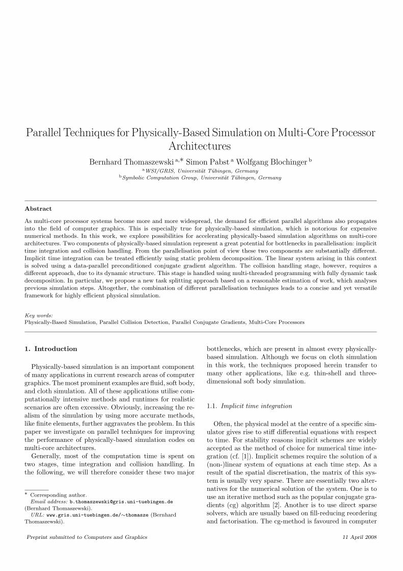
In order to provide context, we will start with a briefoverview of the simulation loop. Fig. 1 shows a schematicview of the simulation loop as used in our specific im-plementation. The simulation starts with an initialisationstage in which meshes for deformable and non-deformableobjects are loaded and bounding volume hierarchies areconstructed. Each iteration of the loop begins with the as-sembly of the linear system of equations arising from theimplicit time integration scheme. Technically, this amountsto assembling the matrix and the right hand side of thesystem. The basis for parallel matrix assembly is the do-main partitioning described in Sec. 4.1. The actual parallelimplementation simply corresponds to the sequential algo-rithm applied to each partition in parallel. The entries ofthe matrix are computed according to the underlying phys-ical model. The next step is the solution of the system withthe method of conjugate gradients, which will supply uswith candidate nodal velocities. The preconditioner is firstupdated with the current matrix data before the iterationstarts. The parallel version of this operation follows againdirectly from the problem decomposition. Each iterationof the cg-method involves the application of the precondi-tioner (pc apply) as well as sparse matrix vector multipli-cation (spmv). Note that for the sake of brevity, we omitfurther operations, such as dot products, which need to becarried out in each iteration step. After convergence, we areprovided with updated nodal velocities and compute newpositions.

The updated positions are then passed on as candidatepositions to the collision handling stage, where they areused to update the bounding volumes. Subsequently, thecollision detection scheme is invoked and intersection-preventing responses are generated as required. Collisionhandling is usually invoked after numerical time integra-tion, but it can also be directly integrated into the solutionof the linear system (see [1]). This stage yields the final,collision-free nodal positions and velocities, which are usedas the initial values for the next step of the simulationloop. Lastly, the final positions are also used to create out-put geometry for visualisation. The following subsectionsdescribe the key steps in greater detail.

3.2. Physical Model and Kinematics

Creating an animation amounts to computing snapshotsof the geometry in the scene at discrete instants in time. Welet x(t+h) stand for the discrete sampling of the nodal tra-jectories x(t), where h is the time step and bold face lettersdenote discrete vectorial quantities. Point-wise kinematicscan be cast as a sequence of coupled initial value problems

3

Fig. 1. Schematic view of the simulation loop according to our implementation. A grey background denotes the components that have beenparalellised. The computationally most expensive parts are printed in bold face.

x(t+h) = x(t) +∫ t+h

t

v(t) dt (1)

v(t+h) = v(t) +∫ t+h

t

a(t) dt,

where v and v(t) denote discrete and continuous nodal ve-locities, respectively. The nodal accelerations a(t) are read-ily related to forces f(t), using Newton’s second law. Theactual way in which these integral equations are trans-formed to discrete algebraic equations depends on the nu-merical time integration scheme. In any case, a method tocompute the internal nodal forces f(t) at a given time t isrequired and we refer to it as the physical model.

The basis for the physical model used in our implementa-tion is a continuum mechanics formulation of linear elastic-ity theory [18]. The central quantities in this case are strain,which is a dimensionless deformation measure, and stress,which is a resulting force per area. These two variables arerelated to each other through a material law, which in ourcase is simply linear. The resulting partial differential equa-tion is discretised using a linear finite element approach asdescribed in [19]. For dynamic simulation, inertia effectshave to be included, as well as viscosity and possibly exter-nal forces.

3.3. Numerical Time Integration

The stiffness of the differential equations (1) suggestsusing implicit numerical time integration. We adopt thefirst order accurate implicit Euler scheme, which seeks tofind v(t+h) and x(t+h) such that

v(t+h) = v(t) + h M−1(f(t,x(t+h),v(t+h)) + fext) (2)

x(t+h) = x(t) + h v(t + h) .

Here, M denotes the diagonal mass matrix and fext ac-counts for external forces like gravity. Note that the inter-nal forces f are evaluated at the end of the time step, giv-ing rise to a system of implicit equations. Generally, f is anonlinear function in terms of x and v and the system hasto be solved using Newton’s method. Anyhow, this breaks

down to repeatedly solving linear systems. In our particularcase, Eq. (2) can be cast into a formulation which is linearwith respect to positions and velocities (see [19]). Hence,we need only solve one linear system per time step. The ac-tual parallel solution of this system using the cg-method isdescribed in Sec. 4.

3.4. Collision Handling

Collision Detection. As a first step, possible interferenceshave to be detected for the deformable objects in the scene.Since all objects are represented as polygonal meshes, thiscould be accomplished by testing every pair of primitives,i.e. polygons, geometrically for intersection. Because the av-erage runtime of this naive approach is unacceptably high,bounding volume hierarchies are usually used for acceler-ation [20]. In this way, non-intersecting parts are quicklyruled out for a given object pair. Such hierarchies consistof two components: a tree representing the topological sub-division of the object into increasingly finer regions andbounding volumes enclosing the geometry associated withevery node in the tree. In our implementation we use dis-crete oriented polytopes (k-DOPs) as bounding volumes(see [21,22]).Testing two objects for interference using bounding volumehierarchies is a recursive process. First, the bounding vol-umes associated with the roots of the two hierarchies aretested for intersection. Only if they overlap, are the respec-tive children tested recursively against each other. Finally,the leaves of the tree need to be checked for intersection us-ing exact geometric tests. If a test signals close proximityor intersection, an appropriate collision response has to begenerated.

Collision Response. Generally speaking, the task of thecollision response stage is to prevent intersections. Thereare various methods for achieving this, ranging from mo-tion constraints over repulsion forces to stopping impulses.Constraints are simple to enforce and do a good job when itcomes to preventing intersections with external objects in

4

rather simple scenes. However, releasing constraints is usu-ally cumbersome and often leads to nodes being arbitrarilyfixed at some point in space. This is particularly disturbingfor self-collisions and literally breaks the simulation.

In our implementation we therefore use a combination ofrepelling forces and stopping impulses (see [23]). If the dis-tance between two approaching objects falls below a certainthreshold, we apply a repulsion force. If the objects can-not be stopped in this way during the next few time steps,we apply stopping impulses, which reliably prevent immi-nent intersections. While this is a straightforward conceptin the sequential case, there are some important implica-tions for parallel implementations. We will discuss these is-sues in Sec. 5. Collision response to complex self-collisionsoften leads to secondary collisions, which also need to behandled to enable high quality simulations. If, after thefirst iteration of the collision handling phase, there are stillremaining or newly introduced collisions, we handle thoseand do another collision detection step, until all collisionsare resolved.

The output of the collision handling stage are new nodalvelocities, which are then finally used to advance the systemto the next time step, i.e., to compute new, collision-freenodal positions. This update is efficiently carried out inparallel using simple loop-level parallelism.

4. Parallel Solution of Sparse Linear Systems

In the following we assume a sparse linear system of theform Ax = b, which is to be solved numerically usingthe cg-method. The iteration stops when the norm of theresidual has been decreased by a given factor (e.g., between10−6 and 10−8 in our case) compared to the initial norm.The number of necessary iterations and therefore the speedof convergence depends on the condition number of thematrix A. Usually, this condition number is improved usinga preconditioning matrix P leading to a modified system

P−1Ax = P−1b,

where P−1A is supposed to have a better condition num-ber and P−1 is fairly easy to compute. The choice of anappropriate preconditioner is crucial because it can reducethe iteration count substantially.

The setup and solution of the linear system now breaksdown to a sequence of operations in which (due to their com-putational complexity) the sparse matrix vector (spmv)multiplication and the application of the preconditionerare most important. Before we discuss these operations inmore detail, we will first describe the underlying problemdecomposition, which forms the basis for the actual paral-lelisation.

4.1. Problem Decomposition

As a basis for the following discussion, we assume thecompressed row storage format for sparse matrices in which

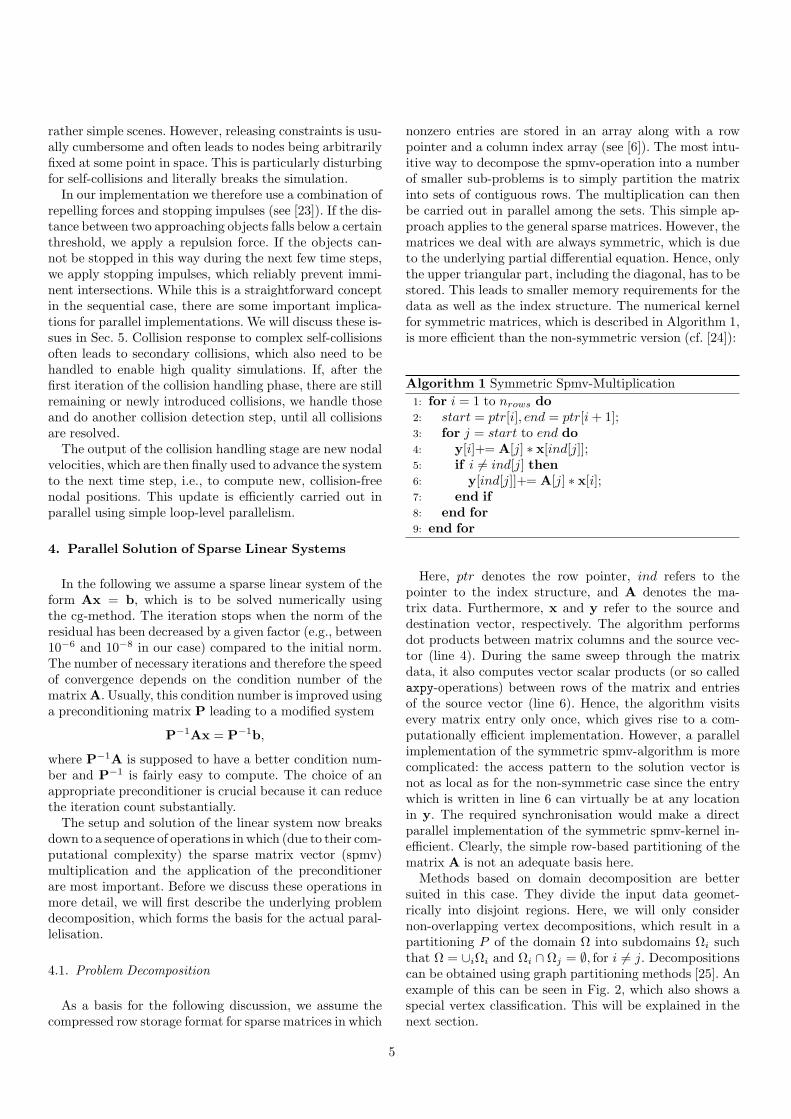
nonzero entries are stored in an array along with a rowpointer and a column index array (see [6]). The most intu-itive way to decompose the spmv-operation into a numberof smaller sub-problems is to simply partition the matrixinto sets of contiguous rows. The multiplication can thenbe carried out in parallel among the sets. This simple ap-proach applies to the general sparse matrices. However, thematrices we deal with are always symmetric, which is dueto the underlying partial differential equation. Hence, onlythe upper triangular part, including the diagonal, has to bestored. This leads to smaller memory requirements for thedata as well as the index structure. The numerical kernelfor symmetric matrices, which is described in Algorithm 1,is more efficient than the non-symmetric version (cf. [24]):

Algorithm 1 Symmetric Spmv-Multiplication1: for i = 1 to nrows do2: start = ptr[i], end = ptr[i + 1];3: for j = start to end do4: y[i]+= A[j] ∗ x[ind[j]];5: if i 6= ind[j] then6: y[ind[j]]+= A[j] ∗ x[i];7: end if8: end for9: end for

Here, ptr denotes the row pointer, ind refers to thepointer to the index structure, and A denotes the ma-trix data. Furthermore, x and y refer to the source anddestination vector, respectively. The algorithm performsdot products between matrix columns and the source vec-tor (line 4). During the same sweep through the matrixdata, it also computes vector scalar products (or so calledaxpy-operations) between rows of the matrix and entriesof the source vector (line 6). Hence, the algorithm visitsevery matrix entry only once, which gives rise to a com-putationally efficient implementation. However, a parallelimplementation of the symmetric spmv-algorithm is morecomplicated: the access pattern to the solution vector isnot as local as for the non-symmetric case since the entrywhich is written in line 6 can virtually be at any locationin y. The required synchronisation would make a directparallel implementation of the symmetric spmv-kernel in-efficient. Clearly, the simple row-based partitioning of thematrix A is not an adequate basis here.

Methods based on domain decomposition are bettersuited in this case. They divide the input data geomet-rically into disjoint regions. Here, we will only considernon-overlapping vertex decompositions, which result in apartitioning P of the domain Ω into subdomains Ωi suchthat Ω = ∪iΩi and Ωi ∩ Ωj = ∅, for i 6= j. Decompositionscan be obtained using graph partitioning methods [25]. Anexample of this can be seen in Fig. 2, which also shows aspecial vertex classification. This will be explained in thenext section.

5

Fig. 2. Decomposition of a mesh into four disjoint partitions indicatedby different colours. The vertex ordering and the resulting matrix

structure for one of the partitions are shown to the right. The matrixAloc describes the internal coupling of the nodes belonging to the

partition (depicted as a square block). The dashed lines indicate the

matrix entries corresponding to boundary vertices of the partition.The rectangular matrix Aext describes the coupling between internal

and external interface nodes.

4.2. Parallel Sparse Matrix Vector Multiplication

Let ni,loc be the number of local vertices belonging to par-tition i and let Vi be the set of corresponding indices. Thesevertices can be decomposed into nint internal vertices andnbnd interface or boundary vertices, which are adjacent tonext vertices from other partitions (see Fig. 2). If we reorderthe vertices globally such that vertices in one partition areenumerated sequentially, we obtain again a partitioning ofthe matrix into a set of contiguous rows. The rows ai,0 toai,n of matrix A where i ∈ Vi have the following specialstructure: the set of entries defined by alm|l ∈ Vi,m ∈ Viforms a symmetric submatrix Ai,loc lying on the diagonalof A. The nonzero entries in this block describe the inter-action between the local nodes of partition i. More specif-ically, this means that when nodes l and m are connectedby an edge in the mesh, there is a nonzero entry alm in thecorresponding submatrix of A. Apart from this symmetricblock on the diagonal there are further nonzero entries ale

where l ∈ Vi is an interface node and e /∈ Vi. These entriesdescribe the coupling between the local interface nodes andneighbouring external nodes.

The matrix vector multiplication can be carried out ef-ficiently in parallel if we adopt the following local vertexnumbering scheme (cf. [6]). The local vertices are reorderedsuch that all internal nodes precede the interface nodes.For further performance enhancement, a numbering schemethat exploits locality (such as a self avoiding walk [9]) canbe used to sort the local vertices. Then, external interfacenodes from neighbouring partitions are locally renumberedas well. Let Aext be the matrix which describes the cou-pling between internal and external interface nodes for agiven partition. Notice that Aext is a sparse rectangularmatrix with nbnd rows. With this setup the multiplicationproceeds as follows:

(i) y(0, nloc) = Aloc · x(0, nloc)

(ii) y(nint, nloc) = y(nint, nloc) + Aext · xext(0, next)

The first operation is a symmetric spmv-multiplication,the second one is a non-symmetric spmv-multiplication fol-lowed by an addition. Both these operations can be carriedout in parallel among all partitions. This decomposition isnot only used for the spmv-kernel but also as a basis forthe parallel matrix assembly as well as for the parallel pre-conditioner, which will be presented next.

4.3. Parallel Preconditioning

In order to make the cg-method fast, it is indispensableto use an efficient preconditioner. There are a broad vari-ety of different preconditioners ranging from simple diago-nal scaling (Jacobi preconditioning) to sophisticated mul-tilevel variants. For an actual choice one has to weigh thetime saved from the reduced iteration count against thecost for setup and repeated application of the precondi-tioner. Additionally, one has to take into account how wella specific preconditioner can be parallelised. Unfortunately,designing efficient preconditioners is usually the most dif-ficult part in the parallel cg-method [7]. As an example,the Jacobi preconditioner is very simple to set up and ap-ply, even in parallel, but the reduction of necessary itera-tions is rather limited. Preconditioners based on (usuallyincomplete) factorisation of the matrix itself or an approx-imation of it are more promising. One example from thisclass is the Symmetric Successive Overrelaxation (SSOR)preconditioner. It is fairly cheap to set up and leads to thesolution of two triangular systems. For the sequential case,this preconditioner has proven to be a good choice in termsof efficiency [26]. However, parallelising the solution of thetriangular systems is very difficult. Even if it is not possibleto decouple the solution of the original triangular systemsinto independent problems we can devise an approximationwith the desired properties. Let A be the block diagonalmatrix with block entries Aii = Ai,loc (see Fig. 2). Visu-ally, the external matrices Aext are dropped from A to giveA. Setting up the SSOR-preconditioner on this modifiedmatrix leads again to the solution of two triangular sys-tems. However, solving these systems breaks down to thesolution of decoupled triangular systems corresponding tothe Ai,loc blocks on the diagonal. This means that they canbe carried out in parallel for every partition.

Approximating A with A means a loss of information,which in turn leads to an increased iteration count. The ac-tual overhead resulting from this approximation dependson the number of partitions used for the problem decompo-sition. Hence, the increased parallelism has to be weighedagainst this additional overhead when deciding on an ac-tual number of partitions. For our experiments we gener-ally set the number of partitions equal to the number ofcores available (see subsequent discussion). For this spe-cific choice the incurred overhead remains small comparedto the speedup obtained through parallelisation.

6

Fig. 3. A comparison of performance obtained for single and double precision arithmetic. The diagram shows sequential runtimes (left),parallel runtimes (middle), and corresponding speedups (right) obtained for preconditioner application (pc apply) and sparse matrix vector

multiplication (spmv) on the three test platforms.

4.4. Parallel Efficiency Considerations

There are further important aspects that have to betaken into consideration in order to set up an efficient par-allel implementation of the cg-method. Dense matrix mul-tiplications usually scale very well since they have regularaccess patterns to memory and a high computational in-tensity per data reference. For the spmv-kernel, however,the picture is quite different. Considering the structure ofthis kernel (see Algorithm 1), it can be seen that the actualmatrix data, as well as the index structure, are traversedlinearly while accesses to the data of the source vector andthe data of the destination vector occur in a non-contiguousfashion, i.e., the locality of these data accesses cannot be as-sumed. The performance of the spmv-algorithm is thereforemostly limited by memory latency and bandwidth, as wellas cache performance. As a result, only a fraction of the the-oretical peak performance for floating point operations canbe attained for the cg-method on a given machine. Accord-ing to Vuduk et al. [27] this fraction is often less than 10%.This dependence is even more pronounced for multi-coreprocessors, where typically two or more cores share a singlememory interface. It is therefore important to improve datalocality and thus cache performance. One way to achievebetter locality is to exploit the natural block layout of thematrix as determined by the underlying partial differentialequation: the coupling between two vertices is described bya 3×3 block – therefore nonzero entries in the matrix alwaysoccur in blocks. Using a block data layout already leadsto a significant improvement. Additional benefits can beachieved using single precision floating point data insteadof double precision. This reduces the necessary matrix data(not including index structure) transferred from memoryby a factor of two. In order to determine the resulting per-formance benefit experimentally, we use a simple test caseas a synthetic benchmark. The input for this test is a flatelastic surface with very high resolution (91,200 vertices).The surface is first isotropically stretched by a factor of1.05 and then released at the beginning of the simulation.For simplicity, gravity was turned off for this test. Since thesurface remains perfectly flat, collisions do not occur andcollision handling was therefore deactivated. We used fourpartitions for the problem decomposition and four threadsfor parallel computations. In order to reduce the overallcomputation time we simulated only 1/30 seconds in this

test. Nevertheless, this period is long enough to capturethe numerical performance since it includes roughly 1300preconditioner applications and spmv-operations.

The results of this experiment are summarised in Dia-gram 3 (see Appendix A for a detailed description of thesystems used). The measurements for the sequential runsalready reveal some interesting aspects. The application ofthe preconditioner is computationally more expensive thanthe spmv-operation on all three systems. This is not sur-prising since both operations are called in every iteration ofthe cg-method and one preconditioner application, involv-ing the solution of two triangular system, is more expensivethan one spmv-operation. The diagram also shows that theperformance difference between single and double precisionis not very pronounced. This rather unexpected behaviourcould be the manifestation of very effective latency hidingby the CPUs and the compiler. Moreover, neither alter-native can consistently outperform the other on all threesystems. Considering the parallel timings, however, we canconclude that the single precision variant performs consis-tently better on all systems. The corresponding speedupvalues are shown on the right in Diagram 3. Depending onthe actual system, a performance gain between 2.0 and 3.7for the preconditioner application and even 3.4 to 3.7 forthe spmv-operation can be obtained for single precision.The speedup values for double precision are not as goodon all three systems and, in particular, there is virtually nospeedup for system 3. We conjecture that this is due to thefact that the four cores of system 3 share a single memoryinterface.

In conclusion, the parallel timings obtained for this ex-periment suggest that single precision arithmetic shouldgenerally be preferred over double precision. In conse-quence, the remaining investigations as well as the nu-merical experiments are solely based on single precisionarithmetic.

In the following section we will discuss some implemen-tation related issues, which have to be considered in orderto implement the single precision variants of the algorithmsin a stable way.

Using Single Precision Floating Point Data In engineer-ing applications absolute accuracy is often of utmost im-portance. It is therefore mandatory to use double preci-sion arithmetic for the numerical algorithms resulting from

7

finite element discretisations. For the case of physically-based simulation in computer graphics, however, visualquality is usually more important than absolute numeri-cal accuracy. For our cloth simulator, we found that, withonly minor modifications, even the largest examples led tono problems using single precision arithmetic. There are,however, a few pitfalls to avoid. The critical arithmetic op-erations where accuracy might potentially be lost are notdivisions or multiplications but additions and subtractionswhere so called cancellation occurs. This can be illustratedwith a simple example: Consider the following sequence ofsummations

a = b + c, d = a− c,

where b = 10−7 and c = 10. Using a 32-Bit single precisiondata type for the variables involved, the numerical resultis d = 0 where it should be d = 10−7. This behaviourcan be explained by considering the definition of this datatype. Assuming the IEEE754 standard, a single precisionfloating point value consists of 1 bit sign s, 23 bit mantissam and 8 bit exponent p, leading to the representation f =(−1)s ·m ·2p (see the standard for more precise definitions).Therefore, if, for a large summand f1 = m1 ·2p1 and a smallsummand f2 = m2 · 2p2 , it holds that

2−23 · 2p1 > m2 · 2p2 ⇔ p1 − p2 > 23,

then the small summand will be absorbed in the summa-tion, i.e. f1 + f2 = f1. Generally, such situations cannotbe avoided in advance since the relative sizes of the sum-mands are not known. However, in many cases it is eitherpossible to reorder summations by hand or to resort to dou-ble precision floating point data for intermediate results.In our implementation, for example, we reordered arith-metic operations for the singular value decomposition of a2×2 matrix necessary for extracting rotations from the dis-placement field (see [19]). Furthermore, we eliminated ac-curacy concerns in the computation of the bending forces,involving trigonometric functions and square root opera-tions (see [28]), by using double precision for intermedi-ate results. Another example is the computation of inter-nal forces which can be done as f = Ku, where K is thestiffness matrix and u = x− x0 is the vector of nodal dis-placements defined as the difference between current po-sitions x and rest positions x0. For technical reasons weoriginally separated this expression into the sequence f =Kx − Kx0. Although convenient when using double pre-cision, we found that this degrades accuracy when usingsingle precision floating point arithmetic. We therefore re-arranged this expression and compute the displacement ufirst, before carrying out matrix multiplication.

In summary, switching to single precision arithmetic re-quires only a few modifications to yield a stable implemen-tation. In particular, we did not encounter any accuracydegradations or convergence problems for the solution ofthe linear system of equations.

Influence of the Number of Threads and Partitions Whensetting up the problem decomposition for solutions of the

linear system of equations, the intuitive choice for the num-ber of partitions is to use as many as there are cores avail-able in the parallel system. For distributed memory systemsthis one-to-one correspondence is often the only practicallyrealisable choice. Furthermore, a partition count exceedingthe number of nodes in a cluster would result in an increasein communication, which is usually prohibitively expensivein the context of distributed memory computing.

Shared memory parallel systems are not as restrictivein terms of communication costs such that using a highernumber of partitions can be considered. In fact, memorylatency may actually be hidden using more partitions thanavailable cores. Additionally, it may be beneficial to adjustthe number of partitions in such a way that the data (orworking set) for a single partition fits into the cache of pro-cessors. We tested the influence of this parameter experi-mentally using the synthetic benchmark described above.The performance differences were, however, rather smalland no improvements could be obtained by using partitioncounts higher than four.

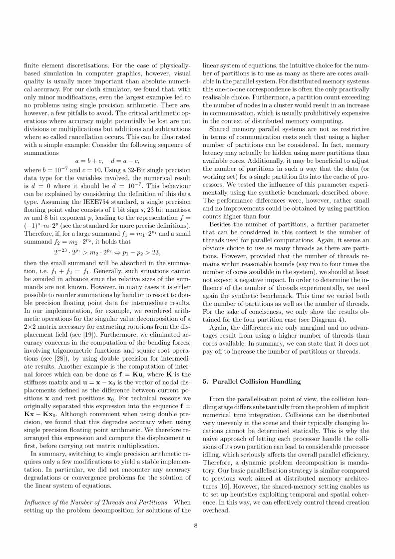
Besides the number of partitions, a further parameterthat can be considered in this context is the number ofthreads used for parallel computations. Again, it seems anobvious choice to use as many threads as there are parti-tions. However, provided that the number of threads re-mains within reasonable bounds (say two to four times thenumber of cores available in the system), we should at leastnot expect a negative impact. In order to determine the in-fluence of the number of threads experimentally, we usedagain the synthetic benchmark. This time we varied boththe number of partitions as well as the number of threads.For the sake of conciseness, we only show the results ob-tained for the four partition case (see Diagram 4).

Again, the differences are only marginal and no advan-tages result from using a higher number of threads thancores available. In summary, we can state that it does notpay off to increase the number of partitions or threads.

5. Parallel Collision Handling

From the parallelisation point of view, the collision han-dling stage differs substantially from the problem of implicitnumerical time integration. Collisions can be distributedvery unevenly in the scene and their typically changing lo-cations cannot be determined statically. This is why thenaive approach of letting each processor handle the colli-sions of its own partition can lead to considerable processoridling, which seriously affects the overall parallel efficiency.Therefore, a dynamic problem decomposition is manda-tory. Our basic parallelisation strategy is similar comparedto previous work aimed at distributed memory architec-tures [16]. However, the shared-memory setting enables usto set up heuristics exploiting temporal and spatial coher-ence. In this way, we can effectively control thread creationoverhead.

8

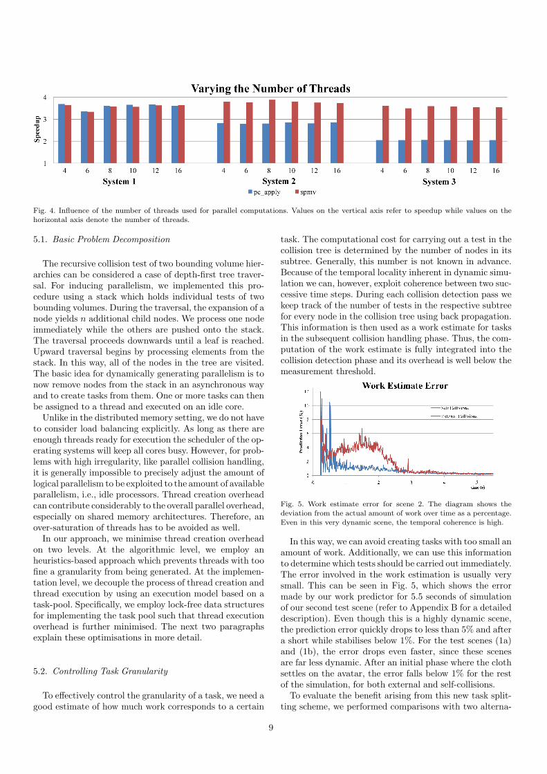
Fig. 4. Influence of the number of threads used for parallel computations. Values on the vertical axis refer to speedup while values on the

horizontal axis denote the number of threads.

5.1. Basic Problem Decomposition

The recursive collision test of two bounding volume hier-archies can be considered a case of depth-first tree traver-sal. For inducing parallelism, we implemented this pro-cedure using a stack which holds individual tests of twobounding volumes. During the traversal, the expansion of anode yields n additional child nodes. We process one nodeimmediately while the others are pushed onto the stack.The traversal proceeds downwards until a leaf is reached.Upward traversal begins by processing elements from thestack. In this way, all of the nodes in the tree are visited.The basic idea for dynamically generating parallelism is tonow remove nodes from the stack in an asynchronous wayand to create tasks from them. One or more tasks can thenbe assigned to a thread and executed on an idle core.

Unlike in the distributed memory setting, we do not haveto consider load balancing explicitly. As long as there areenough threads ready for execution the scheduler of the op-erating systems will keep all cores busy. However, for prob-lems with high irregularity, like parallel collision handling,it is generally impossible to precisely adjust the amount oflogical parallelism to be exploited to the amount of availableparallelism, i.e., idle processors. Thread creation overheadcan contribute considerably to the overall parallel overhead,especially on shared memory architectures. Therefore, anover-saturation of threads has to be avoided as well.

In our approach, we minimise thread creation overheadon two levels. At the algorithmic level, we employ anheuristics-based approach which prevents threads with toofine a granularity from being generated. At the implemen-tation level, we decouple the process of thread creation andthread execution by using an execution model based on atask-pool. Specifically, we employ lock-free data structuresfor implementing the task pool such that thread executionoverhead is further minimised. The next two paragraphsexplain these optimisations in more detail.

5.2. Controlling Task Granularity

To effectively control the granularity of a task, we need agood estimate of how much work corresponds to a certain

task. The computational cost for carrying out a test in thecollision tree is determined by the number of nodes in itssubtree. Generally, this number is not known in advance.Because of the temporal locality inherent in dynamic simu-lation we can, however, exploit coherence between two suc-cessive time steps. During each collision detection pass wekeep track of the number of tests in the respective subtreefor every node in the collision tree using back propagation.This information is then used as a work estimate for tasksin the subsequent collision handling phase. Thus, the com-putation of the work estimate is fully integrated into thecollision detection phase and its overhead is well below themeasurement threshold.

Fig. 5. Work estimate error for scene 2. The diagram shows thedeviation from the actual amount of work over time as a percentage.

Even in this very dynamic scene, the temporal coherence is high.

In this way, we can avoid creating tasks with too small anamount of work. Additionally, we can use this informationto determine which tests should be carried out immediately.The error involved in the work estimation is usually verysmall. This can be seen in Fig. 5, which shows the errormade by our work predictor for 5.5 seconds of simulationof our second test scene (refer to Appendix B for a detaileddescription). Even though this is a highly dynamic scene,the prediction error quickly drops to less than 5% and aftera short while stabilises below 1%. For the test scenes (1a)and (1b), the error drops even faster, since these scenesare far less dynamic. After an initial phase where the clothsettles on the avatar, the error falls below 1% for the restof the simulation, for both external and self-collisions.

To evaluate the benefit arising from this new task split-ting scheme, we performed comparisons with two alterna-

9

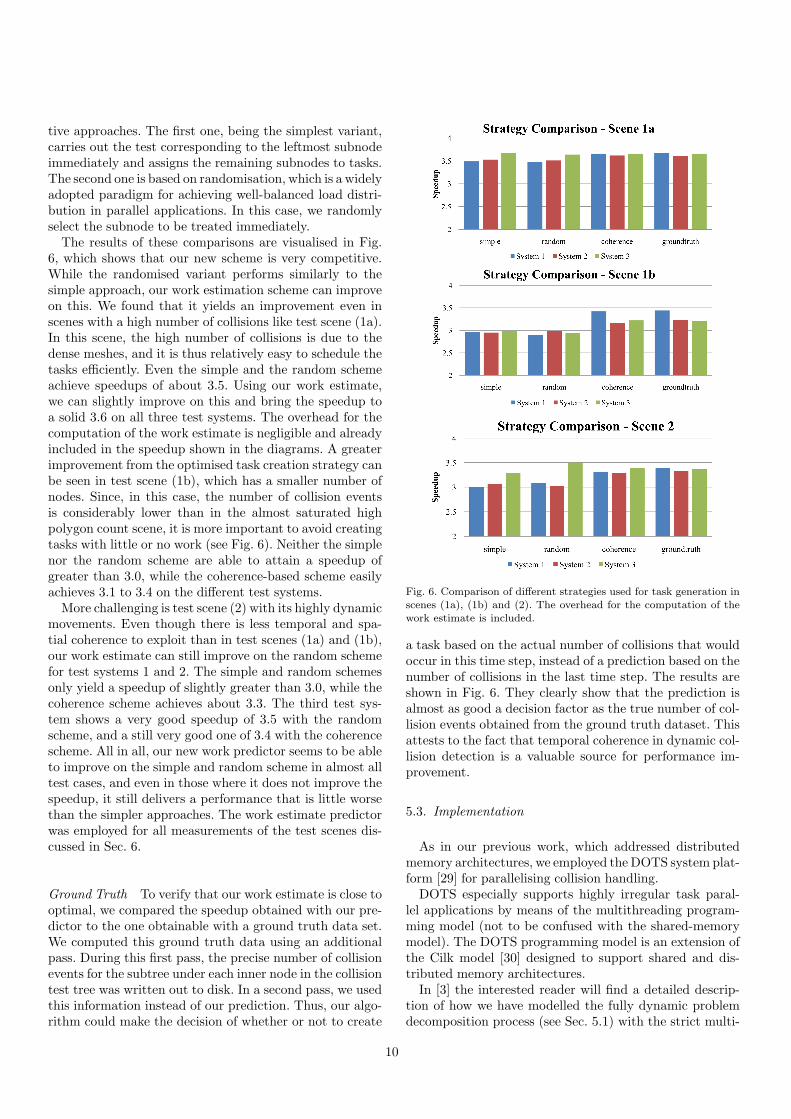
tive approaches. The first one, being the simplest variant,carries out the test corresponding to the leftmost subnodeimmediately and assigns the remaining subnodes to tasks.The second one is based on randomisation, which is a widelyadopted paradigm for achieving well-balanced load distri-bution in parallel applications. In this case, we randomlyselect the subnode to be treated immediately.

The results of these comparisons are visualised in Fig.6, which shows that our new scheme is very competitive.While the randomised variant performs similarly to thesimple approach, our work estimation scheme can improveon this. We found that it yields an improvement even inscenes with a high number of collisions like test scene (1a).In this scene, the high number of collisions is due to thedense meshes, and it is thus relatively easy to schedule thetasks efficiently. Even the simple and the random schemeachieve speedups of about 3.5. Using our work estimate,we can slightly improve on this and bring the speedup toa solid 3.6 on all three test systems. The overhead for thecomputation of the work estimate is negligible and alreadyincluded in the speedup shown in the diagrams. A greaterimprovement from the optimised task creation strategy canbe seen in test scene (1b), which has a smaller number ofnodes. Since, in this case, the number of collision eventsis considerably lower than in the almost saturated highpolygon count scene, it is more important to avoid creatingtasks with little or no work (see Fig. 6). Neither the simplenor the random scheme are able to attain a speedup ofgreater than 3.0, while the coherence-based scheme easilyachieves 3.1 to 3.4 on the different test systems.

More challenging is test scene (2) with its highly dynamicmovements. Even though there is less temporal and spa-tial coherence to exploit than in test scenes (1a) and (1b),our work estimate can still improve on the random schemefor test systems 1 and 2. The simple and random schemesonly yield a speedup of slightly greater than 3.0, while thecoherence scheme achieves about 3.3. The third test sys-tem shows a very good speedup of 3.5 with the randomscheme, and a still very good one of 3.4 with the coherencescheme. All in all, our new work predictor seems to be ableto improve on the simple and random scheme in almost alltest cases, and even in those where it does not improve thespeedup, it still delivers a performance that is little worsethan the simpler approaches. The work estimate predictorwas employed for all measurements of the test scenes dis-cussed in Sec. 6.

Ground Truth To verify that our work estimate is close tooptimal, we compared the speedup obtained with our pre-dictor to the one obtainable with a ground truth data set.We computed this ground truth data using an additionalpass. During this first pass, the precise number of collisionevents for the subtree under each inner node in the collisiontest tree was written out to disk. In a second pass, we usedthis information instead of our prediction. Thus, our algo-rithm could make the decision of whether or not to create

Fig. 6. Comparison of different strategies used for task generation in

scenes (1a), (1b) and (2). The overhead for the computation of the

work estimate is included.

a task based on the actual number of collisions that wouldoccur in this time step, instead of a prediction based on thenumber of collisions in the last time step. The results areshown in Fig. 6. They clearly show that the prediction isalmost as good a decision factor as the true number of col-lision events obtained from the ground truth dataset. Thisattests to the fact that temporal coherence in dynamic col-lision detection is a valuable source for performance im-provement.

5.3. Implementation

As in our previous work, which addressed distributedmemory architectures, we employed the DOTS system plat-form [29] for parallelising collision handling.

DOTS especially supports highly irregular task paral-lel applications by means of the multithreading program-ming model (not to be confused with the shared-memorymodel). The DOTS programming model is an extension ofthe Cilk model [30] designed to support shared and dis-tributed memory architectures.

In [3] the interested reader will find a detailed descrip-tion of how we have modelled the fully dynamic problemdecomposition process (see Sec. 5.1) with the strict multi-

10

threading parallel programming model provided by DOTS.In this section we discuss how we have modified the core

of the run-time system of DOTS in order to further op-timise the execution process on shared-memory architec-tures. Our main design goal was to minimise thread ex-ecution overhead while at the same time keeping all spe-cific functionality of DOTS required to efficiently supporthighly irregular applications, e.g., the decoupling of threadcreation and execution or control of non-determinism.

Basically, DOTS employs lightweight mechanisms formanipulating threads. Forking a thread results in creatinga (passive) thread object, which can later be instantiatedfor execution. Thread objects are either executed by a pre-forked (OS native) worker thread or can be executed ascontinuation of a thread that would otherwise be blocked,e.g., a thread reaching a synchronisation primitive.

The run-time system of DOTS is based on a task pool ex-ecution model. When a thread is spawned (by the dots forkprimitive), the corresponding thread object is placed intoa task pool, which is basically a queue data structure. Onprogram startup, a worker thread is created for each corein the system. Worker threads take thread objects out ofthe task pool and process their run method. In our casethe run method executes the bounding volume hierarchytesting procedure, as discussed in Sec. 5.1. Upon comple-tion of a thread, the corresponding thread object (includ-ing the result of the thread) is placed into a second datastructure called the ready queue. Subsequently, the workerthread gets the next thread object from the task pool andexecutes it. The dots join primitive removes thread objectsfrom the ready queue and delivers the result of the corre-sponding thread to the calling thread. Note that the run-time system of DOTS is only active during the task-parallelcollision handling phase. When program execution is out-side collision handling, the task pool and the ready queueare empty and the worker threads are suspended.

In a shared-memory setting, the task pool and the readyqueue are both concurrently accessed by several threads.The original version of DOTS used mutual exclusion lock-ing primitives for ensuring the consistency of the shareddata structures. In our new approach the task pool andthe ready queue are implemented using lock-free techniques[31].

Lock-free synchronisation is based on an atomic updateoperation, which must be supported by the processor. Thisoperation, commonly referred to as CAS (compare andswap), atomically updates a memory location provided itsinitial content has some expected value. If the value is dif-ferent, the update fails. For example, on the x64 architec-ture family the lock cmpxchg16b instruction provides ap-propriate CAS functionality.

Basically, lock-free techniques employ the CAS operationto realise an optimistic approach for ensuring consistencyof concurrent data structures. A thread loads a value froma shared memory location and stores it in a local variable.The thread now performs a calculation on the local copyresulting in a new value. Finally, the thread tries to update

the original memory location with the CAS instruction,supplying the original and the updated value for compari-son. If the content of the shared memory location has notbeen changed, the update succeeds and the algorithm canproceed. It fails, however, if another thread has updated theshared-memory location during the calculation of the newvalue. In this case, the memory location is re-read and theupdate is tried again with a newly calculated value, untilthe CAS operation succeeds.

In the case of lock-free queues, the shared-memory loca-tion is typically a pointer variable, which is part of a linkedlist. This pointer is updated in order to insert or removea list element. In this context, a subtle problem can occurwhen applying the described techniques. When a memorylocation is reused after the corresponding element has beenremoved from the list the same pointer again becomes partof the list but now represents a different element. How-ever, this change cannot be detected by the CAS operationsince the two elements are represented by the same pointer.Thus, when such a situation occurs during another update,the previous update will be lost. This issue is commonly re-ferred to as the ABA problem. To avoid the ABA problem,reference counters can be associated with pointer variables,which are both compared by the CAS operation. In [32]further details on the implementation of a lock-free queuedata structure are discussed.

Compared to the mutual exclusion approach, lock-freeprogramming reduces overheads since no system calls areneeded for acquiring and releasing locks. Lock-free datastructures also scale well to a larger number of proces-sors/cores since they considerably reduce contention.

We conducted performance measurements to compareour new lock-free approach with the original implementa-tion based on mutual exclusion locks. To assess the effi-ciency of the implementations we determined the executionoverhead of DOTS threads, which is the execution time ofa DOTS thread performing no computation.

Our first test series focuses on latency aspects of threadexecution, which is a measure of the isolated thread ex-ecution overhead. In the corresponding test program onecore forks a thread and immediately joins it. The threadis executed by another idle core. For computing the meanthread execution overhead this fork-join sequence is re-peated 1,000,000 times. The second test series investigatesthroughput aspects of thread execution, which indicatesthe granularity of thread execution. Here, one core forks1,000,000 threads at once, which are concurrently executedby the remaining cores. Fig. 7 shows the resulting meanthread execution overhead for the discussed tests executedon our test systems 2 and 3 (see Appendix A for a detaileddescription). On system 1 the lock cmpxchg16b instructionis not available. However, it has been added on subsequentprocessor generations of the AMD64 architecture, see [33].Thus, the described lock-free techniques cannot be realisedon system 1. For all measurements presented later in thispaper the original version of DOTS (based on mutual ex-clusion locks) has been used for system 1 .

11

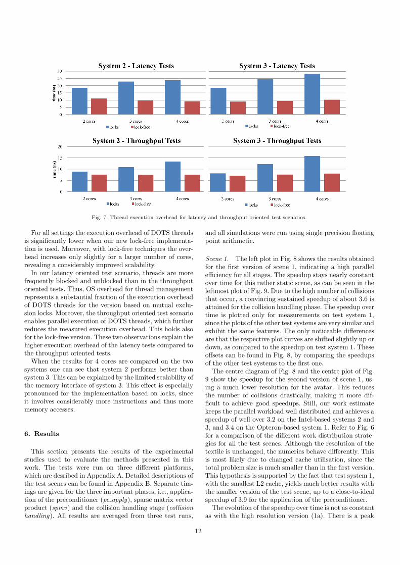
Fig. 7. Thread execution overhead for latency and throughput oriented test scenarios.

For all settings the execution overhead of DOTS threadsis significantly lower when our new lock-free implementa-tion is used. Moreover, with lock-free techniques the over-head increases only slightly for a larger number of cores,revealing a considerably improved scalability.

In our latency oriented test scenario, threads are morefrequently blocked and unblocked than in the throughputoriented tests. Thus, OS overhead for thread managementrepresents a substantial fraction of the execution overheadof DOTS threads for the version based on mutual exclu-sion locks. Moreover, the throughput oriented test scenarioenables parallel execution of DOTS threads, which furtherreduces the measured execution overhead. This holds alsofor the lock-free version. These two observations explain thehigher execution overhead of the latency tests compared tothe throughput oriented tests.

When the results for 4 cores are compared on the twosystems one can see that system 2 performs better thansystem 3. This can be explained by the limited scalability ofthe memory interface of system 3. This effect is especiallypronounced for the implementation based on locks, sinceit involves considerably more instructions and thus morememory accesses.

6. Results

This section presents the results of the experimentalstudies used to evaluate the methods presented in thiswork. The tests were run on three different platforms,which are desribed in Appendix A. Detailed descriptions ofthe test scenes can be found in Appendix B. Separate tim-ings are given for the three important phases, i.e., applica-tion of the preconditioner (pc apply), sparse matrix vectorproduct (spmv) and the collision handling stage (collisionhandling). All results are averaged from three test runs,

and all simulations were run using single precision floatingpoint arithmetic.

Scene 1. The left plot in Fig. 8 shows the results obtainedfor the first version of scene 1, indicating a high parallelefficiency for all stages. The speedup stays nearly constantover time for this rather static scene, as can be seen in theleftmost plot of Fig. 9. Due to the high number of collisionsthat occur, a convincing sustained speedup of about 3.6 isattained for the collision handling phase. The speedup overtime is plotted only for measurements on test system 1,since the plots of the other test systems are very similar andexhibit the same features. The only noticeable differencesare that the respective plot curves are shifted slightly up ordown, as compared to the speedup on test system 1. Theseoffsets can be found in Fig. 8, by comparing the speedupsof the other test systems to the first one.

The centre diagram of Fig. 8 and the centre plot of Fig.9 show the speedup for the second version of scene 1, us-ing a much lower resolution for the avatar. This reducesthe number of collisions drastically, making it more dif-ficult to achieve good speedups. Still, our work estimatekeeps the parallel workload well distributed and achieves aspeedup of well over 3.2 on the Intel-based systems 2 and3, and 3.4 on the Opteron-based system 1. Refer to Fig. 6for a comparison of the different work distribution strate-gies for all the test scenes. Although the resolution of thetextile is unchanged, the numerics behave differently. Thisis most likely due to changed cache utilisation, since thetotal problem size is much smaller than in the first version.This hypothesis is supported by the fact that test system 1,with the smallest L2 cache, yields much better results withthe smaller version of the test scene, up to a close-to-idealspeedup of 3.9 for the application of the preconditioner.

The evolution of the speedup over time is not as constantas with the high resolution version (1a). There is a peak

12

Fig. 8. Integral speedups obtained for test scenes (1a), (1b) and (2). The diagrams show the average speedups of the different stages for bothnumerics and collision handling.

Fig. 9. The plots shows the evolution of the speedups for numerics and collision handling over time, measured for scenes (1a), (1b) and (2)

on System 1.

during the first 300ms of simulation, which correspondsto the cloth settling on the avatar. This initial phase ofthe simulation has a high amount of work for both stagesof the simulation, both numerics and collision handling,and is thus easier to distribute efficiently. Afterwards, thecloth has settled down on the avatar, and both the iterationcount of the cg-method, as well as the number of handledcollisions, goes down, making it harder to find enough workto keep the cores busy.

Scene 2. The rightmost plot in Fig. 8 shows the resultsfor scene (2). Even though this scene exhibits much morecomplicated collisions than the first test scene, particularlywith respect to self-collisions, the speedup of about 3.3 ob-tained for the collision handling stage is not as good as forthe high resolution version of the first test scene. This isdue to the fact that scene (2) is much more dynamic, andthe collisions are distributed more irregularly, making itharder to schedule them efficiently. Our work predictor stillmanages to keep the speedup at a good level of 3.4, but forthis scene we do not improve on the randomised approachfor all test systems. Still, as can be seen from Fig. 6, thedifference is not large and we feel that it is practically morerelevant to achieve good speedups on scenes like (1a) and(1b). The results are also much more consistent when usingour work predictor: all three systems exhibit speedups ofabout 3.3, while with the randomised approach the rangeis from 3.0 for test system 2 to 3.5 for test system 3.

The evolution of the speedup over time plotted in Fig.9 shows a steep increase in the collision handling speedupduring the first second. At the beginning of the simulation,no collisions occur at all, and then as the ribbon falls ontothe inclined plates their number increases rapidly, until af-ter about 1s of simulation time the speedup is at its peak

of 3.5. The numerics speedups stay mostly constant, with asmall peak after about 4s, which corresponds to the ribbonhitting the ground plate. During this impact, the ribbon ex-periences higher deformations leads, which, in turn, resultsin a slightly increased iteration count of the cg-method

7. Conclusions and Future Work

In this work we have presented key techniques for parallelphysically-based simulations on multi-core architectures.We focused on the two major bottlenecks of the simulation,namely the solution of the linear system and the collisionhandling stage, and proposed efficient parallel algorithmsto accelerate these problems. Our performance measure-ments confirm the parallel efficiency of these methods andindicate that physically-based simulations on modern com-modity platforms can be greatly accelerated if parallelism isexploited. Because the scalability is encouraging, we wouldlike to further explore these methods using more processors.Furthermore, we envisage transferring our framework to ahierarchically structured parallel environment, in which thenodes of a distributed memory cluster are each symmetricmulti-processor machines with multiple cores.

8. Acknowledgements

The second author was supported by DFG grant STR465/21-1. The third author was supported in part by theOhio Supercomputer Center. We also thank our reviewersfor their constructive critique.

13

Appendix A. Test Systems

Because the aim of this work is to accelerate computa-tions for physically-based simulations on commodity plat-forms, we decided to use systems that are easily availableat the current time. In order to show that our approachis general and not limited to a specific type of multi-coresystem, we carried out the tests on three different systems.All computers are equipped with 4 CPUs of similar clockspeeds, but differ in their approach to multi-processing.Comparing the scaling on three distinct platforms shouldcreate useful data points, as compared to just analysing asingle platform.

# Architecture Cores L2 Cache RAM

1 AMD Opteron 2×2@2.00Ghz 4×1MB 2GB

2 Intel Xeon 2×2@2.33Ghz 2×4MB 4GB

3 Intel Core2 1×4@2.40Ghz 2×4MB 2GB

Table A.1Systems used for performance experiments

System 1. The first system is based on a dual AMDOpteron 270 (Italy) machine with 2GB of main memory.Each of the Opterons is a dual core processor running at2.0GHz. The memory architecture is shared address-space,more specifically cc-NUMA (cache-coherent-NUMA). EachOpteron core has 1MB of dedicated L2 cache.

System 2. The second platform is a dual Intel Xeon 5140(Woodcrest) running at 2.33GHz and equipped with 4GBof main memory. Again, each of the CPUs is a dual coreprocessor, but each core has access to a much larger unifiedL2 cache of 4MB. It is based on a classic SMP (symmet-ric multi-processor) system, but has an additional memorybus. This means that both of the dual-core processors havetheir own dedicated memory interface.

System 3. The third test platform is an Intel Core 2 QuadQ6600 (Kentsfield) running at 2.40GHz equipped with 2GBof main memory. Again, each core has access to 4MB ofunified L2 cache, for a total of 8MB on die L2 cache. Com-pared to the second system an important difference is thatthe four cores share a single memory interface. As a result,the total memory bandwidth is approximately half that ofthe Woodcrest-based system. This characteristic may havea negative impact on the overall performance when it comesto memory-intensive applications.

Appendix B. Test Scenes

We tested our approach with two scenes, which highlightdifferent aspects of the simulation. Since the focus is on ac-celerating commonly used scenarios, we decided to use onlymoderately large input data. This is an important differ-ence to the distributed memory setting, which traditionally

aims at problem sizes exceeding the capacity of a singleworkstation.

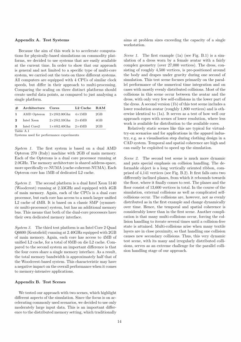
Scene 1. The first example (1a) (see Fig. B.1) is a sim-ulation of a dress worn by a female avatar with a fairlycomplex geometry (over 27,000 vertices). The dress, con-sisting of roughly 4,500 vertices, is pre-positioned aroundthe body and drapes under gravity during one second ofsimulation. This test scene focuses primarily on the paral-lel performance of the numerical time integration and oncases with mostly evenly distributed collisions. Most of thecollisions in this scene occur between the avatar and thedress, with only very few self-collisions in the lower part ofthe dress. A second version (1b) of this test scene includes alower resolution avatar (roughly 1,800 vertices) and is oth-erwise identical to (1a). It serves as a test of how well ourapproach copes with scenes of lower resolution, where lesswork is available for distribution to the available cores.

Relatively static scenes like this are typical for virtual-try-on scenarios and for applications in the apparel indus-try, e.g. as a visualisation step during clothing design in aCAD system. Temporal and spatial coherence are high andcan easily be exploited to speed up the simulation.

Scene 2. The second test scene is much more dynamicand puts special emphasis on collision handling. The de-formable object is a long vertically oriented ribbon, com-prised of 4,141 vertices (see Fig. B.2). It first falls onto twodifferently inclined planes, from which it rebounds towardsthe floor, where it finally comes to rest. The planes and thefloor consist of 13,600 vertices in total. In the course of thesimulation, external collisions as well as complicated self-collisions occur. The collisions are, however, not as evenlydistributed as in the first example and change dynamicallyover time. Hence, the temporal and spatial coherence isconsiderably lower than in the first scene. Another compli-cation is that many multi-collisions occur, forcing the col-lision handling to iterate several times until a collision-freestate is attained. Multi-collisions arise when many textilelayers are in close proximity, so that handling one collisioncauses new secondary collisions. Thus, this very dynamictest scene, with its many and irregularly distributed colli-sions, serves as an extreme challenge for the parallel colli-sion handling stage of our approach.

14

References

[1] D. Baraff, A. Witkin, Large steps in cloth simulation, in:Proceedings of ACM SIGGRAPH ’98, 1998, pp. 43–54.

[2] J. R. Shewchuk, An introduction to the conjugate gradient

method without the agonizing pain, Tech. Rep. CS-94-125,Carnegie Mellon University, Pittsburgh, PA, USA (1994).

[3] B. Thomaszewski, W. Blochinger, Physically based simulation ofcloth on distributed memory architectures, Parallel Computing

33 (6) (2007) 377–390.[4] B. Thomaszewski, S. Pabst, W. Blochinger, Exploiting

parallelism in physically-based simulations on multi-core

processor architectures, in: Proc. of Eurographics Symposium

on Parallel Graphics and Visualization, 2007, pp. 69–76.[5] S. Balay, K. Buschelman, V. Eijkhout, W. D. Gropp, D. Kaushik,

M. G. Knepley, L. C. McInnes, B. F. Smith, H. Zhang, PETScusers manual, Tech. Rep. ANL-95/11 - Revision 2.1.5, Argonne

National Laboratory (2004).[6] Y. Saad, Iterative Methods for Sparse Linear Systems, 2nd

Edition, SIAM, 2003.[7] J. Demmel, M. Heath, H. van der Vorst, Parallel numerical linear

algebra, in: Acta Numerica 1993, Cambridge University Press,

Cambridge, UK, 1993, pp. 111–198.[8] D. O’Hallaron, Spark98: Sparse matrix kernels for shared

memory and message passing systems, Tech. Rep. CMU-CS-97-

178, Carnegie Mellon University, School of Computer Science

(1997).[9] L. Oliker, R. Biswas, P. Husbands, X. Li, Effects of ordering

strategies and programming paradigms on sparse matrixcomputations, Siam Review 44 (3) (2002) 373–393.

[10] S. Romero, L. F. Romero, E. L. Zapata, Fast cloth simulation

with parallel computers, in: Proc. 6th International Euro-ParConference on Parallel Processing, Lecture Notes In Computer

Science, 2000, pp. 491–499.[11] R. Lario, C. Garcia, M. Prieto, F. Tirado, Rapid parallelization

of a multilevel cloth simulator using OpenMP, in: Proc. Third

European Workshop on OpenMP, 2001, pp. 21–29.[12] E. Gutierrez, S. Romero, L. F. Romero, O. Plata, E. L. Zapata,

Parallel techniques in irregular codes: cloth simulation as case

of study, Journal of Parallel and Distributed Computing 65 (4)(2005) 424–436.

[13] F. Zara, F. Faure, J.-M. Vincent, Physical cloth animation ona PC cluster, in: Proc. of Fourth Eurographics Workshop on

Parallel Graphics and Visualization, 2002, pp. 105–112.[14] F. Zara, F. Faure, J.-M. Vincent, Parallel simulation of

large dynamic system on a PCs cluster: Application to cloth

simulation, International Journal of Computers and Applications

26 (3) (2004) 173–180.[15] M. Keckeisen, W. Blochinger, Parallel implicit integration

for cloth animations on distributed memory architectures, in:Proc. of Eurographics Symposium on Parallel Graphics and

Visualization, 2004, pp. 119–126.[16] B. Thomaszewski, W. Blochinger, Parallel simulation of cloth

on distributed memory architectures, in: Proc. of Eurographics

Symposium on Parallel Graphics and Visualization, 2006, pp.35–42.

[17] A. Mujahid, K. Kakusho, M. Minoh, Y. Nakashima, S. Mori,S. Tomita, Simulating realistic force and shape of virtualcloth with adaptive meshes and its parallel implementation inOpenMP, in: Proc. of Intl. Conf. on Parallel and Distributed

Computing and Networks (PDCN2004), 2004, pp. 386–391.[18] P. G. Ciarlet, Mathematical Elasticity. Vol. I, North-Holland

Publishing Co., 1992.[19] O. Etzmuß, M. Keckeisen, W. Straßer, A fast finite element

solution for cloth modelling, in: Proc. 11th Pacific Conference

on Computer Graphics and Applications, 2003, pp. 244–251.[20] M. Teschner, B. Heidelberger, D. Manocha, N. Govindaraju,

G. Zachmann, S. Kimmerle, J. Mezger, A. Fuhrmann, Collision

handling in dynamic simulation environments, in: Eurographics

Tutorials, 2005, pp. 79–185.

[21] J. T. Klosowski, M. Held, J. S. B. Mitchell, H. Sowizral, K. Zikan,Efficient collision detection using bounding volume hierarchies

of k-DOPs, IEEE Transactions on Visualization and Computer

Graphics 4 (1) (1998) 21–36.[22] J. Mezger, S. Kimmerle, O. Etzmuß, Hierarchical techniques in

collision detection for cloth animation, Journal of WSCG 11 (2)

(2003) 322–329.[23] R. Bridson, R. P. Fedkiw, J. Anderson, Robust treatment of

collisions, contact, and friction for cloth animation, in: Proc. of

ACM SIGGRAPH, 2002, pp. 594–603.[24] B. C. Lee, R. W. Vuduc, J. W. Demmel, K. A. Yelick,

Performance models for evaluation and automatic tuningof symmetric sparse matrix-vector multiply, in: Proc. of

International Conference on Parallel Processing (ICPP’04),

2004, pp. 169–176.[25] G. Karypis, V. Kumar, Multilevel k-way partitioning scheme for

irregular graphs, Journal of Parallel and Distributed Computing

48 (1) (1998) 96–129.[26] M. Hauth, O. Etzmuß, A high performance solver for the

animation of deformable objects using advanced numerical

methods, Computer Graphics Forum 20 (3) (2001) 319–328.[27] R. Vuduc, J. Demmel, K. Yelick, S. Kamil, R. Nishtala, B. Lee,

Performance optimizations and bounds for sparse matrix-vector

multiply, in: Proc. of ACM/IEEE Supercomputing, 2002, p. 26.[28] R. Bridson, S. Marino, R. Fedkiw, Simulation of clothing with

folds and wrinkles, in: Proc. of ACM SIGGRAPH/EurographicsSymposium on Computer Animation (SCA 2003), 2003, pp. 28–

36.

[29] W. Blochinger, W. Kuchlin, C. Ludwig, A. Weber, An object-oriented platform for distributed high-performance Symbolic

Computation, Mathematics and Computers in Simulation 49 (3)

(1999) 161–178.[30] K. H. Randall, Cilk: Efficient multithreaded computing, Ph.D.

thesis, MIT Department of Electrical Engineering and Computer

Science (Jun. 1998).[31] J. M. Mellor-Crummey, M. L. Scott, Algorithms for scalable

synchronization on shared-memory multiprocessors, ACM

Transactions on Computer Systems 9 (1) (1991) 21–65.[32] M. M. Michael, M. L. Scott, Simple, fast, and practical non-

blocking and blocking concurrent queue algorithms, in: Proc.of the 15th ACM Symposium on Principles of Distributed

Computing, 1996, pp. 267–275.

[33] Advanced Micro Devices, AMD64 Architecture ProgrammersManual Volume 3: General-Purpose and System Instructions

(2007).

15

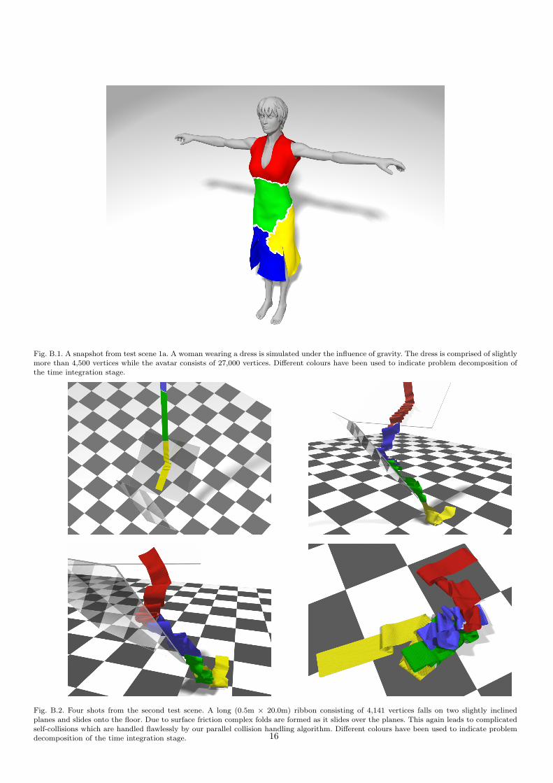
Fig. B.1. A snapshot from test scene 1a. A woman wearing a dress is simulated under the influence of gravity. The dress is comprised of slightly

more than 4,500 vertices while the avatar consists of 27,000 vertices. Different colours have been used to indicate problem decomposition of

the time integration stage.

Fig. B.2. Four shots from the second test scene. A long (0.5m × 20.0m) ribbon consisting of 4,141 vertices falls on two slightly inclinedplanes and slides onto the floor. Due to surface friction complex folds are formed as it slides over the planes. This again leads to complicatedself-collisions which are handled flawlessly by our parallel collision handling algorithm. Different colours have been used to indicate problem

decomposition of the time integration stage. 16