Parallel Computing 49 (2015) 28–49

Contents lists available at ScienceDirect

Parallel Computing

journal homepage: www.elsevier.com/locate/parco

Parallelization of a color-entropy preprocessed Chan–Vese

model for face contour detection on multi-core CPU and GPU

Xiaohua Shi a,c, Fredrick Park b, Lina Wang a, Jack Xin c,∗, Yingyong Qi c

a State Key Laboratory of Software Development Environment, School of Computer Science and Engineering, Beihang University, Beijing, Chinab Department of Mathematics, Whittier College, CA 90601, USAc Department of Mathematics, University of California, Irvine, CA 92697-3875, USA

a r t i c l e i n f o

Article history:

Received 28 February 2014

Revised 22 May 2015

Accepted 15 July 2015

Available online 21 July 2015

Keywords:

Face detection

Color-entropy preprocessing

Chan–Vese segmentation model

Parallelization

a b s t r a c t

Face tracking is an important computer vision technology that has been widely adopted in

many areas, from cell phone applications to industry robots. In this paper, we introduce a

novel way to parallelize a face contour detecting application based on the color-entropy pre-

processed Chan–Vese model utilizing a total variation G-norm. This particular application is

a complicated and unsupervised computational method requiring a large amount of calcu-

lations. Several core parts therein are difficult to parallelize due to heavily correlated data

processing among iterations and pixels.

We develop a novel approach to parallelize the data-dependent core parts and significantly

improve the runtime performance of the model computation. We implement the parallelized

program on OpenCL for both multi-core CPU and GPU. For 640 ∗ 480 input images, the par-

allelized program on a NVidia GTX970 GPU, a NVidia GTX660 GPU, and an AMD FX8530 8-

core CPU is on average 18.6, 12.0 and 4.40 times faster than its single-thread C version on the

AMD FX8530 CPU, respectively. Some parallelized routines have much higher performance

improvement compared to the whole program. For instance, on the NVidia GTX970 GPU, the

parallelized entropy filter routine is on average 74.0 times faster than its single-thread C ver-

sion on the AMD FX8530 8-core CPU. We discuss the parallelization methodologies in detail,

including the scalability, thread models, as well as synchronization methods for both multi-

core CPU and GPU.

© 2015 Elsevier B.V. All rights reserved.

1. Introduction

Face detection is a fundamental computer vision task where the goal is to determine if there are any faces in a given image, and

if so, return the image location and associated pixels corresponding to the face. This particular problem has been one of the most

studied topics in computer vision. Despite being a relatively easy problem for humans, it is exceedingly difficult for computers to

detect faces due to variations in scale, pose, location, orientation, facial expression, illumination, and occlusions. Face detection

can be thought of as the first step in a tracking application which is and of itself an important problem in computer vision.

Technology stemming from the face tracking problem has many practical uses and has been widely adopted in areas varying

from cell phone applications all the way to industry robots. Different methodologies have been applied to this technology and the

∗ Corresponding author. Tel.: +1 949 8245309; fax: +1 949 8247993.

E-mail addresses: xhshi@buaa.edu.cn (X. Shi), fepark@whittier.edu (F. Park), binglina.wang@163.com (L. Wang), jxin@math.uci.edu (J. Xin), yqi@uci.edu

(Y. Qi).

http://dx.doi.org/10.1016/j.parco.2015.07.002

0167-8191/© 2015 Elsevier B.V. All rights reserved.

X. Shi et al. / Parallel Computing 49 (2015) 28–49 29

approaches come from many disciplines. For example, OpenCV uses Haar feature-based cascade classifiers for object detection

to track human front faces, with the support of a proper amount of training data [30], while another recent face tracking method

by Xiong and Torre [42] uses a supervised descent method (Newton’s) for minimizing a non-linear least squares function. We

refer the reader to [20,23,27,36,40,46,47] and references therein for some work on both face detection and tracking.

We develop an unsupervised method for face contour detection by combining skin color, entropy filtering, multi-scale sam-

pling, and the Chan–Vese segmentation model with total variation G-Norm (CVG model) [3,11,12]. The main idea with this ap-

proach is to utilize feature information to guide the final face segmentation step in an accurate manner. The color-entropy pre-

processed Chan–Vese model with G-norm method that we utilize for this tracking application will be called the CEPCVG program

throughout the remainder of this paper. Comparing with other existing approaches, our method not only detects frontal faces,

but also detects side and multiple faces. A major motivation is the development of an accelerated variational principle based

method. Existing methods in the literature either lack systematic principled treatment or robustness and speeds towards real

time application of face segmentation. Our method accomplished both. The tracking precision and speed only depend on the

computational capability of hardware and software platforms and hence, with the fast improvement of computer architectures,

our method can analogously improve in its performance as well. The primary emphasis of this paper is on the parallelization of

the CEPCVG program. In particular, the CV and CVG models are of great importance in image processing and computer vision

where both models are widely used. A parallelization of these models will be an essential contribution to the literature.

In order to effectively utilize the current multi-core CPU and GPU micro architectures, we must foremost have a parallelized

program, because all the aforementioned methods are naturally designed and implemented in a single-thread methodology,

including ours. Researchers have been studying the parallelization of different face tracking applications, by both hardware and

software means. For instance, Theocharides et al. [39] presented a scalable parallel architecture which performs face detection

using the AdaBoost algorithm. Farrugua et al. [19] presented a parallel architecture for fast and robust face detection implemented

on FPGA hardware. Jin et al. [26] introduced a FPGA-based parallel hardware architecture for real-time face detection as well.

In some other similar object or feature detecting applications, researchers have tried to parallelize them as well. For instance,

Yan et al. [43] implemented a parallelized OpenCL program for Speeded-Up Robust Feature (SURF) algorithm on GPUs and CPUs.

Chen. et al. [16] introduced a way to design and implement an adaptive pipeline parallel scheme (AD-PIPE) for both Scale-

invariant feature transform (SIFT) and SURF to alleviate these limitations on multi-core CPUs.

Although much work has been done on parallelizing different face tracking applications, we still cannot directly inherit means

from them because the CVG model we utilize is completely different than anything used in these previous works. In general,

the CEPCVG program, as described in Section 2, is a complicated application that combines many different image processing

methods. The core part of the program, i.e. the CVG segmentation routine using a Primal Dual Hybrid Gradient (PDHG) Method,

has data dependency between iterations and pixels; therefore, it is difficult to parallelize on any parallel platform.

In this paper, we study how to parallelize the CEPCVG program on OpenCL [31], which is an open royalty-free standard for

general purpose parallel programming across CPUs, GPUs and other processors. We parallelized hotspots that dominate the

execution time instead of every code line in the program, to get the trade-off of productivity and efficiency. We use a novel

approach to parallelize the CVG segmentation routine. For 640 ∗ 480 input images, the parallelized program on a NVidia GTX970

GPU, a NVidia GTX660 GPU and an AMD FX8530 8-core CPU is on average 18.6, 12.0 and 4.40 times faster than its single-thread

C version on the AMD FX8530 CPU, respectively. Some parallelized routines have much higher performance improvement when

comparing to the whole program. For instance, on the NVidia GTX970 GPU, the parallelized entropy filter routine is on average

74.0 times faster than its single-thread C version on the AMD FX8530 8-core CPU. The parallelized routines of the whole program

on NVidia GTX970 GPU, NVidia GTX660 GPU and AMD FX8530 8-core CPU are on average 34.4, 15.48 and 4.85 times faster than

the corresponding routines of the single thread C version on the AMD FX8530 CPU, respectively. We discuss the parallelization

methodologies in detail, including the scalability, thread models, as well as synchronization methods for both multi-core CPU

and GPU.

The rest of this paper is organized as follows. Section 2 introduces the mathematical formulae of the CEPCVG program, as well

as the corresponding pseudo code. Section 3 presents how to parallelize the CEPCVG program in detail. Section 4 demonstrates

performance data of the parallelized program on multi-core CPU and GPU. Section 5 concludes this paper.

2. Color-entropy preprocessed CVG (CEPCVG) program

The CEPCVG program is a face tracking application integrating skin color thresholding, entropy-filtering and convexified

image segmentation. It consists of 5 major steps: (1) illumination equalization using combined retinex and Gray World method,

(2) skin region mask construction combining three thresholding methods on skin color, (3) entropy filter edge detector, (4) chin

identification method, and (5) CVG segmentation using the PDHG method.

2.1. Illumination equalization using combined retinex and gray world

Color balancing is an important preprocessing step for digital facial images to achieve color constancy under different illumi-

nations [24]. Two popular approaches for efficient time applications are (1) the gray world assumption and (2) retinex theory. For

the gray world assumption, one seeks to simply equalize the mean of the red, green, and blue channels respectively in the RGB

color space. On the other hand, the retinex theory of visual color constancy states that the perceived white is tied to maximum

cone signals [29]. In [28], Lam showed that by using a combination of the gray world assumption and retinex, one obtains visually

30 X. Shi et al. / Parallel Computing 49 (2015) 28–49

accurate results in regard to color constancy. The method is both computationally efficient and automatic. Given our end goal of

efficient time face tracking, we utilize this combined method in the CEPCVG program.

First, we extract the R, G, and B channels from the input color image f. Second, we solve for R and B channels in the combined

method. For instance, for the R channel, we solve formulae below:[ ∑∑R2

∑∑R

max (R2) max (R)

][μν

]=

[ ∑ ∑G

max (G)

](1)

[μν

]=

[ ∑∑R2

∑∑R

max (R2) max (R)

]−1[ ∑∑G

max (G)

](2)

Rcb = μR2 + νR (3)

For B channel, we use similar formulae above. At last, we get the final illumination adjusted color image fcb:

fcb = [Rcb, G, Bcb]. (4)

2.2. Skin region mask construction combining three threshold methods

The main idea here is to utilize color intensity based thresholding in three different color spaces to form an indicator function

of skin regions. The skin indicators from each of the three thresholding methods on the color spaces are then fused by a median

filter to form a single skin indicator function. For more details on skin detection based on color spaces we refer the reader to the

two surveys [35,41].

For HSV skin color thresholding we utilize the approach by Atharifard and Ghofrani in [1] where it was noted experimentally

that the H component of skin color is ideally concentrated between 0–0.09 and 0.9–1 value-wise. Thus, to obtain an indicator

region for skin tones in the H channel, one simply obtains the image via the logical operation:

Ht =[(H > 0)And(H < 0.09)

]Or

[(H > 0.9)And(H < 1)

]. (5)

Here, Ht stands for H thresholded.

For detecting skin color in YCbCr color space, we utilize the approach by Chai et al. [7,33,34] and the approach by Atharifard

and Ghofrani in [1]. The authors found that any skin pixel value satisfies the following relationship in the YCbCr color space as

follows:

Cbt = (77 < Cb < 127) (6)

Crt = (133 < Cr < 177) (7)

where Cb and Cr denote the chrominance blue and chrominance red channels respectively, Cbt and Crt stand for them thresholded

respectively.

We utilize the RGB color thresholding scheme devised by Ghimire and Lee [20] where the thresholding parameters have been

determined by statistics on skin colors in RGB space. The operation yielding an indicator mask for skin tone pixels for this scheme

follows as:

f mrgb = [R > 95 And G > 40 And B > 20 And max{R, G, B} − min{R, G < B} > 15 And |R − G| > 15

And R > G And R > B]. (8)

We simply take the median of all three skin tone indicator masks from each color space to form a single indicator. The mask

is then binarized by a secondary thresholding step. Given the skin tone indicator masks from the previous steps above: Cbt, Crt,

fmrgb, Ht, the indicator is simply:

Fm = median(Cbt,Crt, f mrgb, Ht) (9)

Ft = (Fm >= 0.5). (10)

The final indicator mask is a single channel binary image Ft where pixel values of 1 denote those of skin.

At last, we create skin pixel indicator masks in 2-D and 3-D to be used later when constructing the entropy filter edge detector

and initial face indicator region for the CVG model.

2.3. Entropy filter edge detector

For the segmentation process, more accurate results can be obtained if an edge detector or skin tone indicator function is

used. This will allow active contours to stop near boundaries on the face under the segmentation process given that we will be

using an edge detector weighted length minimization term for evolving a curve. We utilize an entropy edge/skin-region indicator

X. Shi et al. / Parallel Computing 49 (2015) 28–49 31

function. It has been shown in [38] that entropy is high in regions of an image that contains structural components like edges,

textures, and features. The skin tone indicator mask fm is multiplied to the gray-scale version of the given image fg to incorporate

skin information into the gray-scale image:

f gm = f m ∗ f g. (11)

The entropy filter is then applied to this image and we keep the upper 40% by thresholding. Thus, the facial regions (in

particular, edges and features) will have values of 0 while non-facial regions will have values of 1. In particular, we found that by

using the entropy filter in this manner has a tendency to amplify edges and skin tone features in the image.

To compute the entropy of a gray scale image, let Vmax be the maximum gray-scale value in a given image patch containing N

total pixels. Denote by ni the i-th histogram count and let hi = ni/N the normalized histogram count. We then define the image

patch entropy as the following:

E = −Vmax∑

i=0

hi log (hi). (12)

2.4. Chin identification method

Chin identification is a difficult problem in computer vision. In general, due to variations in skin tone, facial hair, etc. it is

difficult to robustly identify the exact location of a chin in a facial image. We utilize a simple method that maps an image to

the YIQ color space and then in the in-phase channel I, we isolate the face based on a bounding box of the entropy facial region

detector found in the previous step. We then sum all values in the x-direction which yields a 1-D signal. High points in the signal

correspond to parts of the face, while low points correspond to regions where skin tone is not as uniform, e.g. eyes, mouth, chin.

In order to avoid the cutoff at the top of the face, we search starting from the midpoint on in the signal (corresponding to lower

half of the face). The lowest trough in the 1-D signal will correspond to the chin.

First, we extract the in-phase channel I (YIQ space) from the RGB version of our image. A median filter is applied to remove

any noise.

In the next step, we construct a bounding box to the entropy edge or skin-tone region indicator. This will narrow our search

region for the chin contour. We then sum the intensity values in the x-direction (horizontal) to create a 1-D signal.

In the last step, we cut the signal in half and only view the lower half corresponding to the lower half of the face to better

isolate candidate chin locations. Once this is done, we choose the lowest candidate trough which will be the chin location. Finally,

we cut off the entropy edge detector function below this chin location. This forms a more accurate indicator for the face.

2.5. CVG segmentation using PDHG method

For the segmentation step in our proposed method, we utilize the CVG model by Bresson et al. [3]. This particular model has

many advantages over standard image segmentation models in that it combines an edge based approach with a region based

one. Thus, it is robust to noise but at the same time can accurately capture edges in an image. Moreover, the model is convex and

can be minimized quickly by the recent primal dual hybrid algorithms. Given an initial image f defined on a domain D containing

a region to be segmented that we denote by �, the CVG model seeks to minimize the following energy:

min0≤u≤1

∫D

g(|∇ f |)|∇u| + λ

∫D

{(c1 − f (x))2 − (c2 − f (x))2

}︸ ︷︷ ︸

r1(x,c1,c2)

u(x)dx. (13)

One then sets � ={

x : u(x) ≥ 1/2}

which represents the segmented region. The above optimization problem (13) can be viewed

as searching for the best approximation in the L2 sense to a given image f(x) by a function taking only 2 values. The values

are denoted by c1 and c2 taken on the regions � and D�� the unknowns, respectively. In this application, we set c1 = 0.65

and c2 = 0.05 fixed throughout all experiments. The c1 = 0.65 value matches grayscale skin tone average values after such skin

tones are extracted from the color images via the skin indicator mask seen in Section 2.2. The value c2 = 0.05 matches the black

background outside skin tone regions after extraction. The term ∫Dg(|∇f|)|∇u| denotes an edge weighted perimeter of the region

� and enforces regularity on the boundary that separates the regions where the two values c1 and c2 are taken. The function

g = g(|∇ f |) is an edge detector function on the initial image that takes small values near edges and values approaching 1 away

from edges. The parameter λ controls the balance between data fitting and length regularization of the boundary between

segmented regions and we set it to a fixed value 0.1 throughout all experiments. For more information regarding the Chan–Vese

model and related convex relaxation techniques for its minimization, we refer the reader to [11,12].

The above CVG model (13) has the following equivalent unconstrained split formulation:

minu,v

{Er

1(u, v, c1, c2, λ, α) =∫

D

g(|∇ f |)|∇u| + 1

2θ

∫D

(u − v)2dx + λ

∫D

r1(x, c1, c2)v dx + α

∫D

ν(v)dx

}(14)

where ν(ξ) = max{0, 2|ξ − 12 | − 1} is an exact penalty provided that the constant α is chosen large enough compared to λ. The

penalty term is a way to remove the constraints on u and place them into the functional while the splitting term ensures that

u ≈ v. The splitting allows for a fast minimization method via shrinkage. The splitting parameter θ is fixed to be 0.1 throughout

32 X. Shi et al. / Parallel Computing 49 (2015) 28–49

all experiments for a good balance between accuracy and speed. We refer the reader to [3] for more details on this optimization.

This modified energy Er1 can be minimized by minimizing the subproblems:

1. v being fixed, we search for u as a solution of:

minu

{∫D

g(|∇ f |)|∇u| + 1

2θ

∫D

(u − v)2dx

}, (15)

2. u being fixed, we search for v as a solution of:

minv

{1

2θ

∫D

(u − v)2dx +∫

D

r1(x, c1, c2)v dx + α

∫D

ν(v)dx

}. (16)

The solution to (16) is given by a simple shrinkage scheme:

v = min

{max

{u(x) − θλr1(x, c1, c2), 0

}, 1

}. (17)

The solution to (15) is obtained by a primal-dual hybrid gradient (PDHG) method by Zhu and Chan [48] which we focus on now.

For more information on the PDHG method and variants thereof, we refer the reader to [10]. Related variational models and

algorithms can be found in [2,4–6,8,9,13-15,21,22,25,32,37,45].

The minimization problem in (15) reduces to the Total-Variation-G (TVG) min–max problem:

minu

max�p∈X

{∫D

gu( − div�p ) + 1

2θ

∫D

(u − v)2dx︸ ︷︷ ︸�(u,�p)

}(18)

which becomes:

minu

max�p∈X

�(u, �p ) (19)

where X = {�p : |�p | ≤ 1}. We will optimize (19) in the following two step manner below.

Step 1. Dual step

Fix u = uk and apply one step of projected gradient ascent to the max problem:

max�p∈X

�(uk, �p ). (20)

The projected gradient ascent for the maximization (20) is simply:

�p k+1 = PX(�p k + τk∇uk) (21)

where the projection is obtained by the following operation:

PX(�p ) = �p

max{‖�p‖, 1} . (22)

Gradient ascent is an optimization procedure used to find a max of the functional (20) and the projection is used to ensure

that the candidate maxima �p satisfy |�p | ≤ 1 at each step of the iteration process.

Step 2. Primal step

Fix �p = �p k+1 and apply one step of gradient descent method to the minimization problem:

minu

�(u, �p k+1). (23)

The gradient descent associated to the minimization (23) is given by:

uk+1 = uk(1 − θk) + θk(v − θg( − div�p k+1)). (24)

Gradient descent is an analogous optimization procedure to the ascent one used earlier but to find minima of functionals.

Since the original optimization problem (19) is a min–max type, the main idea in the primal-dual hybrid approach is to al-

ternate between minimization and maximization in order to obtain an optimal solution. Recent provable fast convergence

of the primal dual scheme can be found in [10]. We set both the gradient descent and ascent time-steps θ k and τ k to value

1/8 throughout all experiments.

The final PDHG algorithm is then:

Algorithm PDHG

Step 0. Initialization. Pick u0 and �p 0 ∈ X set k ← 0.

Step 1. Choose step size τk and θk .

Step 2. Updating.

�p k+1 = PX(�p k + τk∇uk) (25)

uk+1 = (1 − θk)uk + θk(v − θg( − div�p k+1)) (26)

Step 3. Terminate if stopping criterion is satisfied; otherwise set k ← k + 1 and return to step 1.

X. Shi et al. / Parallel Computing 49 (2015) 28–49 33

//Step1: Illumination Equalization using Combined Retinex and Gray World Method[R, G, B] = extract_RGB_channel(f)[uR,vR] = solve_R(R, f) ;[uB,vB] = solve_B(B, f) ;[Rcb,Bcb] = cal_rcb_bcb(R, B, uR, vR, uB, vB) ;fcb = get_illumination(f, Rcb, Bcb) ;

//Step2: Skin Region Mask Construction Combining Three Threshold Methods[Ht, Cbt, Crt] = HSV_YCbCr_RGB_colorspace_threshold(fcb)ft = fusing_skin_tone_threshold(Ht, Cbt, Crt, R,G,B);fm = mask_for_CVG(ft) ;fg = grayscale(f) ;

//Step3: Entropy Filter Edge Detectorfgm = prepare_entropy(fg, fm) ;fge = entropy_filter(fgm) ;

//Step4: Chin Identification Methodfgemp = prepare_median_filter(fge) ;fgemm = median_filter(fgemp) ;fgem = chin_identification(fgemm) ;

//Step5: CVG Segmentation using PDHG MethodD = 6 ; //constant, down-sampling scaleFmr = imresize(fmask, D) ;Fb = prepare_Fbr_imresize(f, fmask, fgem) ;Fbr = imresize(Fb, D) ;Fgemr = imresize(fgem, D) ;[Fmr, fr] = prepare_CVG_main(Fmr, Fbr) ;u = CVG_main(Fmr, fr) ;

Fig. 1. Pseudo code of the CEPCVG program.

2.6. Pseudo code of CEPCVG program

Observed in Fig. 1 is the pseudo code for the CEPCVG program. We break down and describe the functions in the pseudo code

and the equations they correspond to.

The function extract_RGB_channel() under Step1 extract R, G , and B channels from the input image. Functions solve_R() and

solve_B() solve for the illumination equalization parameters μ and ν for R and B channels, respectively, as Eq. (2) introduced in

Section 2.1. The function cal_rcb_bcb() calculates the equalized red and blue channels Rcb and Bcb as seen in Eq. (3) respectively.

The function get_illumination() corresponds to Eq. (4), the final equalized color image.

The function HSV _YCbCr_RGB_colorspace_threshold() under Step2 corresponds to Eqs. (5)–(8). The function

f using_skin_tone_threshold() corresponds to Eqs. (9) and (10). The function mask_ f or_CVG() corresponds to the last pro-

cedure that creates skin pixel indicator masks in 2-D and 3-D to be used later. The last function grayscale() that has not been

explicitly introduced in Section 2.2 will generate a gray-scale image for the input image f for later uses.

The function prepare_entropy() under Step3 corresponds to Eq. (11) and entropy_ f ilter() corresponds to Eq. (12), the entropy

filter.

The function prepare_median_ f ilter() under Step4 corresponds to processes before median filter as described in Section 2.4.

After applying a median filter on fgemp, Step4 detects the chin location by calling the function chin_identi f ication().

The function imresize() will be called 3 times in Step5 to down sample previously calculated images with different formats.

The function CVG_main() corresponds to the PDHG algorithm for minimizing the CVG model as described in Section 2.5. In

particular, the function corresponds to Eqs. (21), (22), and (24) which is summarized by Algorithm (2.5). Helper functions

prepare_Fbr_imresize() and prepare_CVG_main() will be called within this step to prepare proper arguments for next routines.

Fig. 2 demonstrates the results of the CEPCVG program for 9 randomly selected input images from the CMU Multi-PIE face

database [17], including front face images, 45 and 90° side face images, etc. We draw contours for pixels larger than 0.5 in the

final output matrix u.

3. Parallelizing CEPCVG program

Fig. 3 demonstrates the average runtime hotspots of the CEPCVG single-thread C program on an AMD FX8530 CPU for

640 ∗ 480 face images in Fig. 2, corresponding to functions in Fig. 1. We can find that the top 3 functions, i.e. entropy_ f ilter(),imresize()(called 3 times), and CVG_main(), dominate about 94% of the total execution time. Our parallelization mainly focuses

34 X. Shi et al. / Parallel Computing 49 (2015) 28–49

Fig. 2. Face images with CEPCVG contours.

on these hotspots. In Fig. 3, illumination_equalization represents all functions under Step1 as shown in Fig. 1. Some functions, like

prepare_CVG_main(), prepare_Fr_imresize(), etc., do not appear in the figure, because they occupy too little execution time, e.g.

less than 1%. In this section, we will introduce how to parallelize these hotspots on multi-core CPU and GPU in detail. We use

OpenCL to parallelize the program, to get a good portability on different micro architectures.

3.1. CVG main routine

The CVG main routine, i.e. function CVG_main() in Fig. 1, is the core part of the whole program, although it is the second top

hotspot on CPU, as shown in Fig. 3. It performs a CVG segmentation using PDHG method and occupies about 29% of the total

execution time. The flowchart of its single-thread C implementation is presented in Fig. 4(a).

Unlike other functions that will be introduced in Sections 3.2 and 3.3, the outermost loop of CVG_main() represents the

number of mathematical iterations, e.g. 2500, instead of pixels. Every iteration takes outputs of previous one as its inputs, i.e. u,

p1, and p2, etc. Within each iteration, we first calculate a helper matrix v from existing u and input image fr. Variable u has the

same initial values as the other input image Fmr. Variables W and H stand for the width and height of input images, respectively.

Second, we use two helper matrices, ux and uy, to save forward differences of u in both X and Y directions. Third, the two helper

matrices will be used to calculate the dual step projection saved in p1 and p2, following the method Step1.DualStep introduced

in Section 2.5. p1 and p2 have zero initial values and will be updated during each main iteration. Then, we calculate backward

differences of p1 and p2 in X and Y directions, and also save results in ux and uy, respectively. At last, we update u with its current

values, as well as v, ux, and uy, following the method Step2.PrimalStep introduced in Section 2.5.

Fig. 5 demonstrates how to calculate forward and backward differences in X and Y directions for a 2-D image. For every

function, it calculates differences in two steps. For instance, f orward_x() first calculates the difference between the current pixel

and its next pixel in row order(X direction) for all pixels excluding four 2-pixel borders, like in Fig. 5(a), and then updates four 2-

pixel borders by copying inner rows or columns to outer ones, like in Fig. 5(b). For other functions, i.e. f orward_y(), backward_x(),and backward_y(), they perform the same steps and calculations as f orward_x() except the difference calculations presented in

Fig. 5(c)–(e), corresponding to the gray part in Fig. 5(a).

From Figs. 4(a) and 5, we can find that the original CVG main routine is hard to be parallelized on a data-parallel platform.

The reasons are, first, unlike the entropy filter function introduced in Section 3.2, the outermost iterations of CVG_main() can

not be partitioned to different threads, because every iteration depends on the results of previous ones. Second, the forward

X. Shi et al. / Parallel Computing 49 (2015) 28–49 35

Fig. 3. Hotspots of the CEPCVG single-thread C program on an AMD FX8530 CPU.

and backward difference routines make the final results of each pixel dependent on others. That means, we can not swap the

outermost and inner loops to calculate every pixel iteratively and independently. At last, the forward and backward difference

routines include many memory operations, and they have totally different structures comparing with other parts of CVG_main()and are hard to be parallelized as well.

In order to fully parallelize the CVG main routine, we need to restructure the innermost loop body to be parallelization-

friend. Fig. 6 presents how to restructure the forward and backward difference routines for a 2-D input image. For every forward

or backward routine, we remove memory copy operations by using pre-calculated indirect index matrices mapping to input

images. The point is, when we update borders of an input image by using methods presented in Fig. 5(b), we do not copy the

calculated inner border pixels to outer border ones but re-calculate the latter ones by using indirect indexes of the corresponding

inner border pixels to get the same results as copying. Although we have to pay extra overheads for the redundant calculations,

we removed memory copy operations and successfully restructured the forward and backward difference routines like other

parts of the main iteration.

Fig. 6 (a) demonstrates the restructured function f orward_x(), corresponding to the whole procedures as shown in Fig. 5(a)

and (b). The restructured f orward_x() goes through the whole input image, instead of the inner part without borders as shown

in Fig. 5(a), and calculates differences by using an indirect matrix indirect_idx, as shown in Fig. 6(e) for a 84 ∗ 110 image. For

other restructured difference routines, i.e. f orward_y(), backward_x(), and backward_y(), they perform the similar process like

Fig. 6(a), except the difference calculations presented in Fig. 6(b)–(d), corresponding to the gray chart in Fig. 6(a).

The indirect index matrices can be calculated out off-line, and only depend on the size of an input image. For instance, Fig. 6(e)

demonstrates the indirect index matrix used by f orward_x() and backward_x() for an 84 ∗ 110 input image, i.e. indirect_idx

in the figure. The first element of the matrix, i.e. indirect_idx[0, 0], equals to indirect_idx[3, 3] that has a linear index value

255 = 3 ∗ 84 + 3, corresponding to the copy operation as shown in Fig. 5(b). Likewise, indexes of all other pixels on borders can

be calculated like the first one. For pixels in the inner part of the image, their indexes are not changed. For instance, for a pixel

with index [4, 3], its linear index value equals to 339 = 4 ∗ 84 + 3. Functions f orward_x() and backward_x() use only one index

matrix like Fig. 6(e), while f orward_y() and backward_y() use one more index matrix indirect_idx_y that can be calculated out

off-line just like indirect_idx in a similar way.

Fig. 4 (b) demonstrates the restructured CVG main routine, by using the restructured forward and backward difference rou-

tines presented in Fig. 6. The restructured C version inlines the four difference routines, as the gray charts shown in Fig. 4(b).

After inlining, the original three inner loops have been reduced to two, with the same loop bound, i.e. the pixel number of the

input image.

It is much easier to parallelize the restructured CVG main routine than the original C implementation. Fig. 4(c) shows the

parallelized OpenCL version based on the restructured function. We assign every pixel of the input image to a thread and cal-

culate its iterations simultaneously. Because of data dependency, we have to place two global synchronizations at the positions

where the restructured function finishes the two inner loops, as the gray charts shown in Fig. 4(c). We implemented the global

synchronization function by using the atomic add function atomic_inc() provided by OpenCL runtime. In theory, the overheads

of synchronizations could be negligible if all threads arrive at their synchronization points concurrently, however, the synchro-

nization overheads could be significantly higher due to asynchronous arrivals and lock operations.

36 X. Shi et al. / Parallel Computing 49 (2015) 28–49

Fig. 4. Flowcharts of function CVG_main().

Although we must perform a global lock for every thread running on CPU, GPU can take advantage of its existing lightweight

branch synchronization mechanism to perform a partial global lock for every workgroup instead of thread, because GPU executes

OpenCL applications in a Single-Instruction Multi-Threading (SIMT) model that could also be regarded as an implicit Single-

Instruction Multi-Data (SIMD) model. For SIMT architectures, one instruction is fetched for a warp of sequential threads and

executed on the SIMD units, thus diverging control flow with thread-dependent conditional branches in the kernel usually results

in low performance because the branches are executed sequentially [44]. Fig. 7 demonstrates a typical branch synchronization

code on GPU, in which the variable lid stands for the unique local work-item ID within a specific workgroup. All threads within

the same workgroup will wait at the end of the branch for others, until they finish all branches in the figure.

Fig. 8 demonstrates the pseudo code of the partial global lock for GPU, by using its branch synchronization mechanism. For

all threads within the same workgroup, we only perform a global lock for the first one, while other threads will automatically

X. Shi et al. / Parallel Computing 49 (2015) 28–49 37

M = Height 4N = Width - 4

i = 0

i < M

j = 0

j < N

dx[2+i,2+j] = u[2+i,3+j] -u[2+i, 2+j]

j = j + 1

i = i +1

return(dx)

M = Height 4N = Width - 4

dx[2~M+1,0] = dx[2~M+1,3]dx[2~M+1,1] = dx[2~M+1,2]

dx[2~M+1,N+2] = dx[2~M+1,N+1]dx[2~M+1,N+3] = dx[2~M+1,N]

dx[0,0~N+3] = dx[3,0~N+3]dx[1,0~N+3] = dx[2,0~N+3]

dx[M+2,0~N+3] = dx[M+1,0~N+3]dx[M+3,0~N+3] = dx[M,0~N+3]

return(dx)

(a) forward_x: step 1 (b) step 2

dx[2+i,2+j] = u[3+i,2+j] -u[2+i, 2+j]

j = j + 1

(c) forward_y: step 1

dx[2+i,2+j] = u[2+i,2+j] -u[2+i, 1+j]

j = j + 1

(d) backward_x: step 1

dx[2+i,2+j] = u[2+i,2+j] -u[1+i, 2+j]

j = j + 1

(e) backward_y: step 1

Fig. 5. Calculating forward and backward differences in X and Y directions.

Fig. 6. Restructured forward and backward difference routines and an indirect index matrix sample for a 84∗110 input image.

if(lid == 0) {repeat128(t1/=t2; t2%=t1;)}else if(lid == 1) {repeat128(t1/=t2; t2%=t1;)}...else if(lid == 31) {repeat128(t1/=t2; t2%=t1;)}

Fig. 7. Sample code of thread-dependent conditional branches.

38 X. Shi et al. / Parallel Computing 49 (2015) 28–49

lid = get_local_id() ;if(is_the_first_thread_within_workgroup(lid)){lock() ;}barrier(CLK_GLOBAL_MEM_FENCE); //global memory fencebarrier(CLK_LOCAL_MEM_FENCE); //local memory fence

Fig. 8. A partial global lock for GPU.

Fig. 9. Flowcharts of function entropy_ f ilter().

wait at the end of the if block for the locked one. Then we will perform two optional memory fences for both global and local

memories for data consistency. This partial global lock has the same function as a full global lock without the if condition on GPU,

with much fewer lock operations. It significantly improves the runtime performance of CVG_main(), as shown in Section 4.

3.2. Entropy filter

The entropy filter function, entropy_ f ilter(), is the topmost hotspot of the single-thread CEPCVG program on the AMD FX8530

CPU. It occupies about 43% of the total execution time, as shown in Fig. 3. It returns an array fge, where each output pixel contains

the entropy value of its 15-by-15 neighborhood around the corresponding pixel in the input image fgm. For pixels on the borders

of fgm, it uses symmetric padding, in which the values of padding pixels are a mirror reflection of the border pixels in fgm. The

input image fgm can have any dimension, while only 2-D dimension is used by our program.

Fig. 9 (a) presents the flowchart of the single-thread C function. It first pads the input image fgm with a larger border and

saves results in fgmp. Then, it goes through every pixel to calculate the histogram for the gray-scale intensity image fgm by using

256 bins. At last, it calculates the entropy value for every input pixel based on the histogram results.

We parallelized the whole function except the padding routine, which mainly performs memory copy operations and only

takes a few milliseconds on CPU. Although the function goes through the 15-by-15 neighborhood of every pixel when calculating

its entropy value, the calculating results of every pixel are totally independent of the results of any other. That means, we can

simply assign every pixel to an OpenCL thread to perform the same calculations simultaneously, without any synchronization,

like Fig. 3(b).

In the parallelized program, the global workgroup size of the OpenCL kernel may have the same value as the input image

fgm. For instance, for a 640 ∗ 480 input image, the global workgroup size could be (640, 480) as well. For multi-core CPU, we

use the default local workgroup size provided by the OpenCL runtime, while it is more complicated for GPU. For fully utilizing

X. Shi et al. / Parallel Computing 49 (2015) 28–49 39

GPU cores, the local workgroup size should not be less than the number of Computing Unit(CU) and the workgroup number

should be a multiple of the number of Processing Element(PE). For instance, NVidia GTX660 GPU has 5 PEs and each PE has 192

CUs. With a fixed global workgroup size (640, 480), the best local workgroup size for the GPU could be (60, 16). That means,

(640 ∗ 480)/(60 ∗ 16) = 320 workgroups will fairly share the 5 PEs, and 60 ∗ 16 = 960 threads within every workgroup will

run on 192 CUs within each PE. Different thread models, i.e. global and local workgroup sizes, may lead to different runtime

performance on CPU and GPU. Section 4 will introduce more in terms of the scalability and thread models of the parallelized

version.

3.3. Resizing image

The CEPCVG C program uses an important helper function, imresize(), to down-sample an input image. The function is called

three times during the execution, and occupies about 22% of the total execution time, see Fig. 3. Fig. 10(a) demonstrates the

flowchart of its single-thread C implementation. First, the function applies a 2-D windowed anti-aliasing filter on the input

image by using a constant Gaussian kernel related to the filter window size. Then, it interpolates the filtered input image in the

Y direction. At last, it interpolates the filtered input image in X direction and outputs the down-sampled image. In the figure,

variables W and H stand for the width and height of the input image, respectively.

Although some open-source libraries, like OpenCV, provide GPU solutions for resizing images, their performance and func-

tionality do not fully meet our demand. We have to implement our own approach to parallelize the routine. Section 4 will

compare the performance of our approach with OpenCV’s GPU solutions.

Because the X direction interpolation uses the outputs of the Y direction interpolation, while the latter one uses the outputs of

the anti-aliasing filter, and all their input images have different sizes, we use 3 different OpenCL kernels to parallelize the whole

routine, like Fig. 10(b). Similar to the function entropy_ f ilter(), the 2-D windowed anti-aliasing filter performs calculations on

every pixel independently of the results of any other. In the same way, we can assign every pixel to an OpenCL thread to perform

the calculations simultaneously, without any synchronization, like Fig. 10(b). We have the similar concerns on thread models of

this kernel for GPU and CPU, like the entropy filter function as well.

The Y direction interpolation down-samples the filtered input image in Y direction with the down-sampling scale. For in-

stance, it down-samples a 640 ∗ 480 image to 640 ∗ 80 with a down-sampling scale value D = 6. The corresponding OpenCL

kernel triggers H/D = 80 threads to perform the down-sampling calculations for every 640-pixel row simultaneously.

The X direction interpolation down-samples the output image of the Y direction interpolation with the same down-sampling

scale. For instance, it down-samples a 640 ∗ 80 input image to 106 ∗ 80 with a down-sampling scale value 6. The corre-

sponding OpenCL kernel triggers W/D = 106 threads to perform the down-sampling calculations for every 80-pixel column

simultaneously.

3.4. Parallelization of other routines

Besides the top three hotspots, some other single-thread C routines can be parallelized as well, although they could not

improve the overall performance so significantly as the former ones. These routines could be divided into two categories, one

is “pixel-independent”, like the aforementioned entropy filter routine, one is “vectorizable”, according to their program struc-

ture features. The pixel-independent category includes functions median_ f ilter(), HSV _YCbCr_RGB_colorspace_threshold(), and

grayscale(), etc. The vectorizable category includes function cal_rcb_bcb(), etc.

• Pixel-independent functions

Function median_ f ilter() performs median filtering for an input 2-D image. It outputs an image with the same size as

the input one. Each output pixel contains the median value in the M-by-N neighborhood around the corresponding pixel

in the input image, with padded zero borders. When filtering binary input images, we use a simplified algorithm to calculate

the median of the M-by-N neighborhood around the corresponding pixel in a linear way, instead of sorting the neighborhood

first, like Fig. 11(a). For any M ∗ N binary values, their median is 1.0 if their sum is larger than M ∗ N/2, or 0.5 if their sum

equals to M ∗ N/2, or 0 if their sum is less than M ∗ N/2, when M ∗ N is even. When M ∗ N is odd, their median is 1.0 if their

sum is not less than (M ∗ N + 1)/2, or 0 in other cases. We can find that every pixel calculates its median value in the M-by-

N neighborhood independently from each other, so we can assign every pixel to different thread and calculate all of them

simultaneously, like Fig. 11(b). So we call them “pixel-independent”.

Like image resizing routine, although some open-source libraries, like OpenCV, provide GPU solutions for median filter, their

performance and functionality do not fully meet our demand. We have to implement our own approach to parallelize the

routine. Section 4 will compare the performance of our approach with OpenCV’s GPU solutions.

Likewise, HSV _YCbCr_RGB_colorspace_threshold() and grayscale() calculate every input pixel independently as well. We use

the similar way to parallelize them also, just like median_ f ilter() or others.• Vectorizable functions

GPU provides powerful vector instructions that have much higher performance comparing with non-vector ones [44]. How-

ever, unlike the ideal cases introduced in micro benchmarks, many CEPCVG routines are not suitable, or not sensitive, for

vectorization. For instance, we tried to use vector operations in the entropy filter function. However, we did not get any

obvious performance improvement by them.

40 X. Shi et al. / Parallel Computing 49 (2015) 28–49

Fig. 10. Flowcharts of function imresize().

In the whole CEPCVG program, one of the most suitable case for vectorization is function cal_rcb_bcb(), as shown in Fig. 1.

The corresponding Eq. (3) is a typical vector calculation formula, so we can use vectors to calculate Rcb and Bcb instead of

single elements. Its parallelization is quite simple, just by assigning different elements or vectors to different threads. We use

vectors with different sizes, from 2 to 8 elements, to evaluate the runtime performance, since different vector sizes may have

different overheads. Section 4 will demonstrate the runtime performance with 2,4, or 8-byte vectors in detail.

X. Shi et al. / Parallel Computing 49 (2015) 28–49 41

Fig. 11. Simplified median filter algorithm for 2-D binary images and its parallelized implementation. Note: cal_med() in (b) is equivalent to the gray charts in

(a).

0

500

1000

1500

2000

2500

3000

ms

Execu

Single-thread C OpenCL on AMD FX8530OpenCL on GTX660 OpenCL on GTX970

Fig. 12. Total execution time of the single-thread C and OpenCL programs for 640∗480 input images on AMD FX8530 8-core CPU, NVidia GTX970 and GTX660

GPUs.

4. Performance evaluation

We evaluated the runtime performance of the single-thread CEPCVG C program on an AMD FX8530 8-core 4.0G CPU, with

4G main memory. The parallelized OpenCL version ran on the same AMD FX8530 CPU, a NVidia GTX970 GPU with 4G on-board

GPU memory, as well as a NVidia GTX660 GPU with 2G on-board GPU memory. The OpenCL platforms are AMD APP SDK V2.7

and NVidia’s OpenCL v1.1 plus CUDA 4.2.9, for the AMD CPU and NVidia CPUs, respectively. The compiler is GCC4.6.2 and the OS

is Ubuntu12.04(Linux ubuntu 2.6.38-13-generic). When we evaluate the runtime performance for the whole CEPCVG program

or routines below, including the CVG main iteration, the entropy filter, the median filter, etc., we count all necessary overheads

including I/O between GPUs and CPU via PCI-E bus. For instance, when we evaluate the runtime performance of the OpenCL

kernel of entropy filter, we count the time before the input buffers are transferred from the host to the device and after the

output buffers are transferred from the device to the host. In general, when we parallelize the CEPCVG algorithm based on the

single-thread C program, we do not change any computational complexity of the original C code. We also evaluated the outputs of

the parallelized program with the original C program for all input images we used. They are all exactly the same, with acceptable

floating point errors produced by different micro architectures, e.g. X86 CPUs and NVidia GPUs.

Fig. 12 demonstrates the runtime performance of the single-thread C and OpenCL CEPCVG programs for 9 640 ∗ 480 input

images shown in Fig. 2, on AMD FX8530 8-core CPU, NVidia GTX970 and GTX660 GPUs, respectively. For the whole program, the

OpenCL version speeds up 18.6, 12.04 and 4.40 times on average, on NVidia GPUs and the AMD multi-core CPU, comparing with

the single-thread C version on the same AMD CPU, respectively.

Because there is little published in the literature in terms of how to parallelize a face segmentation program by using CVG

model on GPU, we compared the performance of our CEPCVG program with the parallelized face detection example based

on Haar feature-based cascade classifiers for object detection of OpenCV 2.4.10, which is implemented on OpenCL as well.

42 X. Shi et al. / Parallel Computing 49 (2015) 28–49

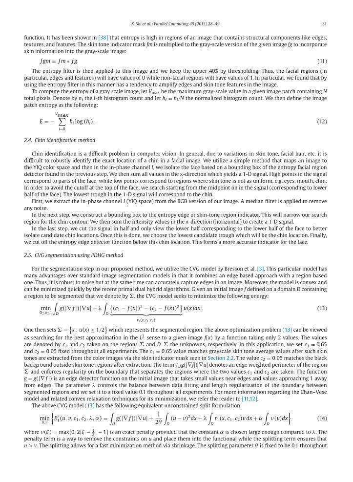
Fig. 13. Face detection results by OpenCV.

0

5

10

15

20

25

F1 F2 F3 F4 F5 F6 F7 F8 F9 Average

Speed-up

OpenCV on GTX970 CEPCVG on GTX970

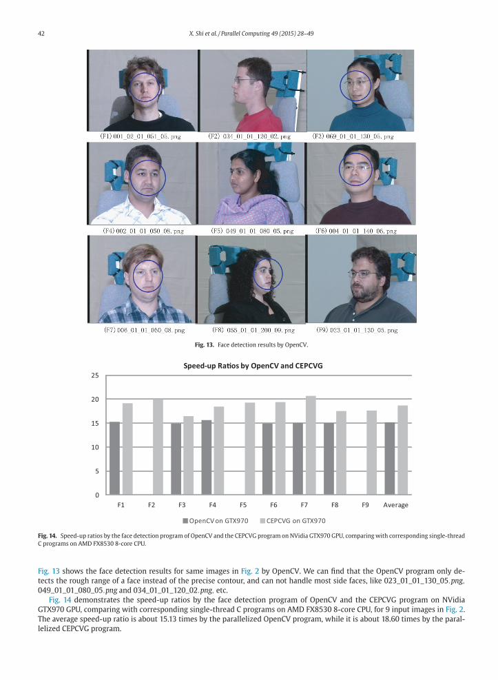
Fig. 14. Speed-up ratios by the face detection program of OpenCV and the CEPCVG program on NVidia GTX970 GPU, comparing with corresponding single-thread

C programs on AMD FX8530 8-core CPU.

Fig. 13 shows the face detection results for same images in Fig. 2 by OpenCV. We can find that the OpenCV program only de-

tects the rough range of a face instead of the precise contour, and can not handle most side faces, like 023_01_01_130_05.png,

049_01_01_080_05.png and 034_01_01_120_02.png, etc.

Fig. 14 demonstrates the speed-up ratios by the face detection program of OpenCV and the CEPCVG program on NVidia

GTX970 GPU, comparing with corresponding single-thread C programs on AMD FX8530 8-core CPU, for 9 input images in Fig. 2.

The average speed-up ratio is about 15.13 times by the parallelized OpenCV program, while it is about 18.60 times by the paral-

lelized CEPCVG program.

X. Shi et al. / Parallel Computing 49 (2015) 28–49 43

0

100

200

300

400

500

600

700

800

F1 F2 F3 F4 F5 F6 F7 F8 F9 Average

ms

Single-thread C OpenCL on AMD FX8530 OpenCL on GTX660, full lock

OpenCL on GTX970, full lock

Fig. 15. Execution time of the single-thread and OpenCL CVG_main() functions for 640∗480 input images on AMD FX8530 8-core CPU , NVidia GTX970 and

GTX660 GPUs.

0

100

200

300

400

500

600

700

800

900

1000

1/1 2/1 4/1 8/1 16/2 32/4

ms.

Global Worksize/Local Worksize

FX8530 CPU

AMD FX8530 8-core CPU Linear Time

0

100

200

300

400

500

600

700

800

ms.

Global Worksize/Local Worksize

NVidia GTX660 GPU

Nvidia GTX660 GPU Linear Time

Fig. 16. Scalability of CVG_main() for the input image 001_02_01_051_05.png on AMD FX8530 8-core CPU and NVidia GTX660 GPU.

Fig. 15 demonstrates the runtime performance of the single-thread and OpenCL versions of CVG_main() for 9 640 ∗ 480 input

images, on AMD FX8530 8-core CPU, NVidia GTX970 and GTX660 GPUs, respectively. On NVidia GPUs and the AMD multi-core

CPU, the parallelized OpenCL function CVG_main() is on average 28.1, 12.18 and 5.22 times faster than the single-thread C version

on the AMD CPU, respectively. As introduced in Section 2, we can use the partial global lock on GPUs to perform synchronizations.

This optimization significantly improves the performance on GTX970 and GTX660 GPUs, about 3.16 and 2.33 times, respectively,

as shown in Fig. 15. However, this optimization does not work on CPUs, because the branch synchronization mechanism does not

exist on this kind of micro architectures [44].

Similar to other functions, we use a 2-dimension global worksize Width ∗ Height and 2-dimension local worksize

((Width/N) ∗ (Height/M)) to run the OpenCL kernel on NVidia GPUs, while the local worksize should be not less than 192 and

N ∗ M not less than 20, to fully utilize GTX970’s 13 PEs and 1664 CUs (128 CUs per PE), and GTX660’s 5 PEs and 960 CUs (192 CUs

per PE). For the AMD FX8530 8-core CPU, we use a 1-D global worksize 32 and local worksize 4 to fully utilize its 8 cores. On CPU,

one thread may handles multiple pixels in a similar way as shown in Fig. 4(c), with two more inner loops corresponding to the

pixel number before the two global synchronizations.

Fig. 16 presents the scalability of CVG_main() for the input image F1 in Fig. 2 on AMD FX8530 8-core CPU and NVidia GTX660

GPU, respectively. The “Linear Time” lines present the linear time values by dividing the initial time of one thread or one group

by workgroup numbers, which are equal to global worksizes divided by local worksizes. Because we down-sample the input

640 ∗ 480 image by a factor 6, as shown in Fig. 1, the input image size of CVG_main() is 110 ∗ 84 with 2-pixel borders. For the

AMD 8-core CPU, we choose different global/local worksizes, like 1/1, 2/1, 16/2, 32/4, to increase the workgroup number from 1

to 8. The OpenCL version achieves linear time improvement when the workgroup number is 2, and is slower than the linear time

line when the workgroup number increases to 4 and 8. However, the gap between the real execution time and the ideal linear

44 X. Shi et al. / Parallel Computing 49 (2015) 28–49

0

200

400

600

800

1000

1200

1400

F1 F2 F3 F4 F5 F6 F7 F8 F9 Average

ms

Single-thread C OpenCL on AMD FX8530 OpenCL on GTX660 OpenCL on GTX970

Fig. 17. Execution time of the single-thread and OpenCL entropy_ f ilter() functions for 640∗480 input images on AMD FX8530 8-core CPU, NVidia GTX970 and

GTX660 GPUs.

0200400600800

100012001400160018002000

ms.

Global Workszie/Local Worksize

Scalability of Entropy Filter on AMD FX8530 8-core CPU

AMD FX8530 8-core CPU Linear Time

050

100150200250300350400450

ms.

Global Worksize/Local Worksize

Scalability of Entropy Filter on NVidia GTX660 GPU

Nvidia GTX660 GPU

Linear Time

Fig. 18. Scalability of entropy_ f ilter() for the input image 001_02_01_051_05.png on AMD FX8530 8-core CPU and NVidia GTX660 GPU.

time does not raise, as shown in Fig. 16. That means, with more CPU cores, the runtime performance of CVG_main() could still

increase.

For the NVidia GTX660 GPU, we increase the workgroup number from 1 to 5, corresponding to its 5 PEs. The OpenCL version

achieves higher performance improvement than linear time and keeps this trend with the increment of the workgroup number.

That means, first, with more GPU cores, the runtime performance of CVG_main() could still increase. Second, when running with

only 1 workgroup, the OpenCL version might encounter some bottlenecks of computing resources, e.g. synchronization, memory

bandwidth, etc., and achieve lower performance than the ideal case.

In fact, Fig. 15 proves the scalability of CVG_main() when we ran the some OpenCL routine on a more powerful GPU than

GTX660. According to NVidia’s official evaluation results [18], GTX970 is on average about 2 times faster than GTX 660 for many

workloads. For CVG_main(), as Fig. 16 shows, GTX970 is on average 2.2 times faster than GTX660.

Fig. 17 demonstrates the runtime performance of the single-thread and OpenCL versions of entropy_ f ilter() for 9 640 ∗ 480

input images, on AMD FX8530 8-core CPU, NVidia GTX970 and GTX660 GPUs, respectively. The parallelized OpenCL function

entropy_ f ilter() is 74.03, 37.59 and 3.72 times faster on average, on NVidia’s GPUs and the AMD multi-core CPU, comparing with

the single-thread C version on the AMD CPU, respectively. We use a 2-dimension global worksize (640 ∗ 480) and 2-dimension

local worksize (16 ∗ 60) to run the OpenCL kernel on NVidia GPUs, to fully utilize their PEs and CUs, for a 640 ∗ 480 input image.

For the AMD FX8530 8-core CPU, we use the same global and local worksizes as GPUs.

Fig. 18 demonstrates the scalability of entropy_ f ilter() on AMD FX8530 8-core CPU and NVidia GTX660 GPU, respectively.

For the AMD 8-core CPU, like CVG_main(), we choose different global/local worksizes, like 1/1, 2/1, 16/2, 32/4, to increase the

X. Shi et al. / Parallel Computing 49 (2015) 28–49 45

0

20

40

60

80

100

120

140

160

180

200

F1 F2 F3 F4 F5 F6 F7 F8 F9 Average

ms

Single-thread C OpenCL on AMD FX8530

OpenCL on GTX660 OpenCL on GTX970

resize() of OpenCV on GTX970

Fig. 19. Execution time of the single-thread and OpenCL imresize() functions for 640∗480 input images on AMD FX8530 8-core CPU , NVidia GTX970 and GTX660

GPUs, as well as the OpenCL resize() function of OpenCV on GTX970.

workgroup number from 1 to 8. For the NVidia GTX660 GPU, we increase the workgroup number from 1 to 5, corresponding to

its 5 PEs. The linear time lines illustrate the ideal time improvement regarding the increment of workgroup numbers. We can

find the OpenCL version almost overlaps the linear time lines on both AMD CPU and NVidia GPU. That means, with more CPU or

GPU cores, the runtime performance of entropy_ f ilter() could still increase.

Fig. 17 proves the scalability of entropy_ f ilter() when we ran the some OpenCL routine on a more powerful GPU than GTX660.

As what aforementioned, GTX970 is on average about 2 times faster than GTX660 for many workloads. For entropy_ f ilter(), as

Fig. 16 shows, GTX970 is on average 1.97 times faster than GTX660.

Fig. 19 demonstrates the runtime performance of the single-thread and OpenCL versions of imresize() for 9 640 ∗ 480 input

images, on AMD FX8530 8-core CPU, NVidia GTX970 and GTX660 GPUs, respectively. The parallelized OpenCL function imresize()

is on average 24.17, 13.74 and 11.72 times faster on NVidia GPUs and the AMD multi-core CPU, comparing with the single-thread

C version on the same AMD CPU, respectively. Fig. 19 also shows the performance of the OpenCL resize() function of OpenCV

2.4.10 by using the same input data. The average execution time of resize() is about 24.8 ms on GTX970, while it is about 7.6 ms

by our approach.

The functions has 3 kernels, as described in Section 3.3, however, the first kernel occupies more than 99% of its total execution

time on both CPU and GPU. We use the same thread configurations as entropy_ f ilter() for the first kernel on the AMD multi-core

CPU and NVidia GPUs. For the second and third kernels, we use Height/D and Width/D as the global worksizes, in which D is

the down-sampling scale, for CPU and GPUs. The local worksize will be chosen by the OpenCL platform automatically for both

processors.

It is interesting that the speed-up number of the OpenCL version of imresize() on the AMD 8-core CPU is even higher than its

core number 8, as shown in Fig. 19. The main reason is, the extra I/O between main memory and GPU on-board memory could

introduce extra overheads while the computing loads are relatively low. Further more, the parallelized OpenCL function could

have much better cache behavior comparing with its single-thread version, and speed the performance up even higher than the

core number.

Fig. 20 demonstrates the runtime performance of the single-thread and OpenCL versions of median_ f ilter() for 9 640 ∗ 480

input images, on AMD FX8530 8-core CPU, NVidia GTX970 and GTX660 GPUs, respectively. The parallelized OpenCL function

median_ f ilter() is on average 4.13, 3.10 and 4.29 times faster on NVidia GPUs and the AMD multi-core CPU, comparing with

the single-thread C version on the same AMD CPU, respectively. Fig. 19 also shows the performance of the OpenCL medianFilter()

function of OpenCV 2.4.10 by using the same input data. The average execution time of medianFilter() is about 25.9 ms on GTX970,

while it is about 7.7 ms by our approach.

It is interesting that the OpenCL kernel runs faster on the AMD 8-core CPU than NVidia GPUs. The main reason is, the extra

I/O between the main memory and GPU on-board memory could introduce obvious overheads while the computing loads are

relatively low. Similar to previous routines, we use a 2-dimension global worksize Width ∗ Height and 2-dimension local worksize

((Width/N) ∗ (Height/M)) to run the OpenCL kernel on NVidia GPUs, to fully utilize their PEs and CUs. For the AMD FX8530 8-core

CPU, we use the same global worksize as the GPU, while the local worksize is automatically chosen by the OpenCL platform.

46 X. Shi et al. / Parallel Computing 49 (2015) 28–49

0

5

10

15

20

25

30

35

F1 F2 F3 F4 F5 F6 F7 F8 F9 Average

ms

Single-thread C OpenCL on AMD FX8530

OpenCL on GTX660 OpenCL on GTX970

medianFilter() of OpenCV on GTX970

Fig. 20. Execution time of the single-thread and OpenCL median_ f ilter() functions for 640∗480 input images on AMD FX8530 8-core CPU, NVidia GTX970 and

GTX660 GPUs, as well as the OpenCL medianFilter() function of OpenCV on GTX970.

4.741

5.751

1.070

1.744

0.156 0.092 0.053 0.057 0.087 0.046 0.024 0.025

0.000 0.500 1.000 1.500 2.000 2.500 3.000 3.500 4.000 4.500 5.000 5.500 6.000

un-vectorized uchar2 uchar4 uchar8

ms

AMD FX8530 8-core CPU NVidia GTX660 GPU NVidia GTX970 GPU

Fig. 21. Execution time of OpenCL kernel cal_rcb_bcb() for the input images 001_02_01_051_05.png with different vector sizes on AMD FX8530 8-core CPU,

NVidia GTX970 and GTX660 GPUs.

We discussed some vectorizable functions in Section 3.4. Although these functions do not obviously improve the whole pro-

gram, the vectorization is still an important optimization on multi-core CPU and GPU. Fig. 21 demonstrates the runtime perfor-

mance of the OpenCL kernel cal_rcb_bcb() with different vector sizes on AMD FX8530 8-core CPU, NVidia GTX970 and GTX660

GPUs, respectively. When we choose uchar4 as the vector size, the OpenCL kernel is 4.43, 3.63 and 2.93 times faster than its

un-vectorized version, on AMD FX8530 8-core CPU, NVidia GTX970 and GTX660 GPUs, respectively.

Fig. 22 presents the average execution time of parallelized and un-parallelized routines for 640 ∗ 480 input images on

AMD FX8530 8-core CPU, NVidia GTX970 and GTX660 GPUs. About 96.24% of the original single-thread C program has been

parallelized in terms of execution time. The parallelized routines occupy about 89.27, 80.36 and 67.82% of the total execu-

tion time on AMD FX8530 8-core CPU, NVidia GTX660 and GTX970 GPUs, respectively. The parallelized routines of the whole

program on NVidia GTX970 GPU, GTX660 GPU and AMD FX8530 8-core CPU are on average 34.4, 15.48 and 4.85 times faster

than the corresponding routines of the single thread C implementation on the AMD FX8530 CPU, respectively. The execu-

tion time of un-parallelized parts may vary after parallelization, due to the change in I/O and memory access behaviors. After

parallelization, hotspots may change on the multi-core CPU and GPUs, as shown in Fig. 23. For instance, the top hotspot on

AMD FX8530 CPU now is entropy_ f ilter() while it is CVG_main() on NVidia GTX970 GPU. That means, if we want to optimize

the OpenCL program further, different parallelization efforts may be paid for different micro architectures, even for the same

program.

X. Shi et al. / Parallel Computing 49 (2015) 28–49 47

2462.00

560.11 204.56 132.33

70.00

67.33

50.00 62.80

Single-thread AMD FX8530 8-core CPU NVidia GTX660 GPU NVidia GTX970 GPU

Time of Parallelized and Un-

Fig. 22. Average execution time of parallelized and un-parallelized routines for 640∗480 input images on AMD FX8530 8-core CPU, NVidia GTX970 and GTX660

GPUs.

Fig. 23. Hotspots for 640∗480 input images on AMD FX8530 8-core CPU and NVidia GTX970 GPU, after parallelization.

5. Conclusions and future work

In this paper, we introduced methodologies to parallelize a face contour detecting application based on the Chan–Vese model

using the total variation G Norm, which is a complicated computational application from applied mathematics that does not

depend on any training data. We discuss how to parallelize one of the core routines, i.e. CVG_main(), which has data dependency

between iterations and pixels and is thus difficult to be parallelized, as well as other hotspots like an entropy filter function and

an image resizing function to name few. We demonstrate the performance data of the parallelized program on multi-core CPU

and GPUs in detail. This is a key contribution given the wide scope and use of the Chan–Vese model in the literature.

When parallelizing such a practical and complicated application, we can not achieve the best performance by simply paral-

lelizing a single algorithm. As what was aforementioned, some trivial helper or I/O functions may dominate the total execution

time after parallelizing existing hotspots, and more engineering efforts might be paid for the remaining work here. Furthermore,

in the core routine CVG_main(), another way to deal with the data dependency between iterations and pixels would be the use

of a parallelized spectral method of which the authors are currently pursuing. Lastly, SIMD instructions and approximate pro-

cessing could be applied to the parallelized implementation on multi-core CPUs, to improve the scalability and vectorization

optimizations.

48 X. Shi et al. / Parallel Computing 49 (2015) 28–49

Acknowledgements

This work was partially supported by a Qualcomm Research Gift to UC Irvine, US NSF grant DMS-1222507, National Natural

Science Foundation of China grants no. 61272166, and the State Key Laboratory of Software Development Environment of China

no.SKLSDE-2014ZX-10. The authors would like to thank Dr. Xiangxin Zhu for helpful discussions.

References

[1] A. Atharifard, S. Ghofrani, Robust component-based face detection using color feature, in: Proceedings of the World Congress on Engineering 2011, in: WCE2011, vol 2, July 6-8, 2011.London, U.K

[2] X. Bresson, T. Chan, Active contours based on Chambolle’s mean curvature motion, IEEE Int. Conf. Image Process. (ICIP ’07) I (2007) 33–36,doi:10.1109/ICIP.2007.4378884.

[3] X. Bresson, E. S, P. Vanderheynst, J.P. Thiran, S. Osher, Fast global minimization of the active contour/snake model, J. Math. Imaging and Vision 28 (2007)151–167, doi:10.1007/s10851-007-0002-0.

[4] X. Cai, R.H. Chan, T. Zeng, A two-stage image segmentation method using a convex variant of the Mumford–Shah model and thresholding, SIAM J. Imaging

Sci. 6 (1) (2013) 368–390.[5] J. Carter, Dual Methods for Total Variation–Based Image Restoration, Dept. Math., UCLA, LA, CA, 2001 Ph.d. disseration.

[6] C. Caselles, R. Kimmel, G. Sapiro, Geodesic active contours, Int. J. Comput. Vis. 22 (1) (1997) 61–79.[7] D. Chai, K.N. Ngan, Face segmentation using skin color map in videophone applications, IEEE Trans. CAS Video Technol. 9 (4) (1999) 551–564.

[8] A. Chambolle, An algorithm for total variation minimization and applications, J. Math. Imaging Vis. 20 (2004) 89–97,doi:10.1023/B:JMIV.0000011321.19549.88.

[9] A. Chambolle, R.A. De Vore, N.T. Lee, B.J. Lucier, Nonlinear wavelet image processing: variational problems, compression, and noise removal through waveletshrinkage, IEEE Trans. Image Process. 7 (1998) 319–335, doi:10.1109/83.661182.

[10] A. Chambolle, T. Pock, A first-order primal-dual algorithm for convex problems with applications to imaging, J. Math. Imaging Vis. 20 (1) (2011) 120–145,

doi:10.1007/s10851-010-0251-1.[11] T.F. Chan, S. Esedoglu, M. Nikolova, Algorithms for finding global minimizers of image segmentation and denoising models, SIAM J. Appl. Math. 66 (2006)

1632–1648, doi:10.1137/040615286.[12] T.F. Chan, L.A. Vese, Active contours without edges, IEEE Trans. Image Process. 10 (2) (2001).

[13] T.F. Chan, G. Golub, P. Mulet, A nonlinear primal-dual method for total variation-based image restoration, SIAM J. Sci. Comput. 20 (1999) 1964–1977,doi:10.1137/S1064827596299767.

[14] T.F. Chan, S. Esedoglu, Aspects of total variation regularized L1 function approximation, SIAM J. Appl. Math. 65 (5) (2005) 1817–1837, doi:10.1137/040604297.

[15] J.S. Chang, E.Y. Kim, H.J. Kim, Facial boundary detection with an active contour model, Pattern Recognit. Lett. 28 (2007) 67–75.[16] P. Chen, D.L. Yang, W.H. Zhang, Y. Li, B.Y. Zang, H.B. Chen, Adaptive pipeline parallelism for image feature extraction algorithms, in: Proceedings of the 41st

International Conference on Parallel Processing (ICPP), 2012, 2012, pp. 299–308.[17] The CMU Multi-PIE Face Database, at URL: http://www.multipie.org/ (last accessed May 18, 2015).

[18] NVidia Geforce GTX970 performance evaluation results, at URL: http://www.geforce.cn/hardware/desktop-gpus/geforce-gtx-970/performance (last ac-cessed May 18, 2015).

[19] N. Farrugia, F. Mamalet, S. Roux, et al., Fast and robust face detection on a parallel optimized architecture implemented on FPGA[J], IEEE Trans. Circuits Syst.

Video Technol. 19 (4) (2009) 597–602.[20] D. Ghimire, J. Lee, A robust face detection method based on skin color and edges, J. Inf. Process Syst. 9 (1) (2013). http://dx.doi.org/10.3745/JIPS.2013.9.1.

141[21] T. Goldstein, X. Bresson, S. Osher, Geometric applications of the split Bregman method: segmentation and surface reconstruction, CAM, LA, CA, 2009. Rep.

09-06[22] T. Goldstein, S. Osher, The split Bregman method for L1-regularized problems, SIAM J. Imaging Sci. 2 (2009) 323–343, doi:10.1137/080725891.

[23] R. Gupta, A.K. Saxena, Survey of advanced face detection techniques in image processing, Int. J. Comput. Sci. Manage. Res. 1 (2) (2012).

[24] R. Hunt, The Reproduction of Colour, 6th edition, Wiley, 2004.[25] M. Kass, A. Witkin, D. Terzopoulos, Snakes: active contour models, Int. J. Comput. Vis. (1987) 321–331.

[26] S. Jin, D. Kim, T.T. Nguyen, et al., An FPGA-based parallel hardware architecture for real-time face detection using a face certainty map[C]//Application-specific systems, in: Proceedings of the 20th IEEE International Conference on Architectures and Processors, ASAP 2009., 2009, pp. 61–66.

[27] M. Kim, S. Kumar, V. Pavlovic, Rowley, Face tracking and recognition with visual constraints in real-world videos, CVPR (2008).[28] E.Y. Lam, Combining gray world and retinex theory for automatic white balance in digital photography, in: Proceedings of the Ninth International Sympo-

sium on Consumer Electronics. 07/2005, in: ISCE 2005, 2005 ISBN: 0-7803-8920-4, doi:10.1109/ISCE.2005.1502356.

[29] E. Land, J. McCann, Lightness and retinex theory, J. Opt. Soc. Am. 61 (1) (1971) 1–11.[30] OpenCV Cascade Classification, at URL: http://docs.opencv.org/modules/objdetect/doc/cascade_classification.html (last accessed May 18, 2015).

[31] OpenCL official site, at URL: http://www.khronos.org/opencl/ (last accessed May 18, 2015).[32] S. Osher, M. Burger, D. Goldfarb, J. Xu, W. Yin, An iterative regularization method for total variation-based image restoration, SIAM Multiscale Model. Simul.

4 (2005) 460–489, doi:10.1137/040605412.[33] S.L. Phung, A. Bouzerdoum, D. Chai, A novel skin color model in YCbCr color space and its application to human face detection, IEEE Int. Image Process. (1)

(2002) 289–292.

[34] S.L. Phung, A. Bouzerdoum, D. Chai, Skin segmentation using color pixel classification: analysis and comparison, IEEE Trans. Pattern Anal. Mach. Intell. 27(1) (2005) 148–154.

[35] C. Prema, D. Manimegalai, Survey on skin tone detection using color spaces, Int. J. Appl. Inf. Syst. (IJAIS) 2 (2) (2012).ISSN : 2249–0868 Foundation ofComputer Science FCS, New York, USA

[36] S. Rivera, A. Martinez, Learning deformable shape manifolds, Pattern Recognit. 45 (4) (2012) 1792–1801.[37] L.I. Rudin, S. Osher, E. Fatemi, Nonlinear total variation based noise removal algorithms, Physica D 60 (1992) 259–268, doi:10.1016/0167-2789(92)

90242-F.[38] Y. Sun, J. Xin, Content adaptive image matching by color-entropy segmentation and inpainting, in: P. Real, et al. (Eds.), Proceedings of the 14th International

Conference on Computer Analysis of Images and Patterns, CAIP 2011, LNCS 6855, Springer-Verlag, 2011, pp. 471–478.

[39] T. Theocharides, N. Vijaykrishnan, M.J. Irwin, A parallel architecture for hardware face detection, in: Proceedings of ISVLSI, 6, 2006, p. 452.[40] S. Tripathi, V. Sharma, S. Sharma, Face detection using combined skin color detector and template matching method, Int. J. Comput. Appl. 26 (7) (2011).

[41] V. Vezhnevets, V. Sazonov, A. Andreeva, A survey on pixel-based skin color detection techniques, in: Proceedings of GRAPHICON, 2003, pp. 85–92.[42] X. Xiong, F. Torre, Supervised descent method and its applications to face alignment, in: Proceedings of IEEE Conference on Computer Vision and Pattern

Recognition, 2013, pp. 533–539.[43] W.L. Yan, X.H. Shi, X. Yan, L.N. Wang, Computing OpenSURF on OpenCL and general purpose GPU, Int. J. Adv. Robot. Syst. 10 (2013) 375–386,

doi:10.5772/57057.

X. Shi et al. / Parallel Computing 49 (2015) 28–49 49

[44] X. Yan, X.H. Shi, L.N. Wang, H.Y. Yang, An OpenCL micro-benchmark suite for GPUs and CPUs, J. Supercomput. (2014), doi:10.1007/s11227-014-1112-2.[45] C. Zach, T. Pock, H. Bischof, A globally optimal algorithm for robust TV-L1 range image integration, in: Proceedings of the 11th IEEE International Conference

on Comput. Vision (ICCV ’07), 1, 2007, pp. 1–8, doi:10.1109/ICCV.2007.4408983.[46] C. Zhang, Z. Zhang, A survey of Recent Advances in Face Detection, Microsoft Research Technical Report MSR-TR-2010-66 (2010).

[47] X. Zhu, D. Ramanan, Face detection, pose estimation, and landmark localization in the wild, in: Proceedings of the CVPR, 2012. Providence RI.[48] M. Zhu, T.F. Chan, An Efficient Primal-Dual Hybrid Gradient Algorithm for Total Variation Image Restoration, CAM, LA, CA, 2008. Rep. 08-34.