parallel scc and centrality - computer science | …slotag/classes/fa16/slides/lec05-web2.pdf ·...
TRANSCRIPT

Parallel SCC and CentralityLecture 5
CSCI 4974/6971
15 Sep 2016
1 / 16

Today’s Biz
1. Quick Review
2. Reminders
3. Parallel SCC
4. More Centrality
5. Even More MPI
6. More PageRank Tutorial
2 / 16
Today’s Biz
1. Quick Review
2. Reminders
3. Parallel SCC
4. More Centrality
5. Even More MPI
6. More PageRank Tutorial
3 / 16
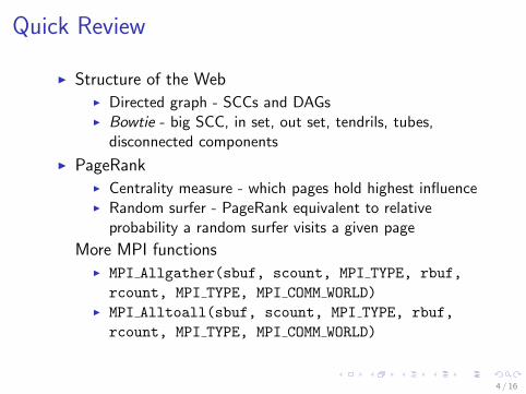
Quick Review
I Structure of the WebI Directed graph - SCCs and DAGsI Bowtie - big SCC, in set, out set, tendrils, tubes,
disconnected components
I PageRankI Centrality measure - which pages hold highest influenceI Random surfer - PageRank equivalent to relative
probability a random surfer visits a given page
More MPI functionsI MPI Allgather(sbuf, scount, MPI TYPE, rbuf,
rcount, MPI TYPE, MPI COMM WORLD)I MPI Alltoall(sbuf, scount, MPI TYPE, rbuf,
rcount, MPI TYPE, MPI COMM WORLD)
4 / 16
Today’s Biz
1. Quick Review
2. Reminders
3. Parallel SCC
4. More Centrality
5. Even More MPI
6. More PageRank Tutorial
5 / 16
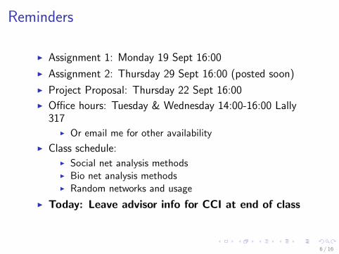
Reminders
I Assignment 1: Monday 19 Sept 16:00
I Assignment 2: Thursday 29 Sept 16:00 (posted soon)
I Project Proposal: Thursday 22 Sept 16:00
I Office hours: Tuesday & Wednesday 14:00-16:00 Lally317
I Or email me for other availability
I Class schedule:I Social net analysis methodsI Bio net analysis methodsI Random networks and usage
I Today: Leave advisor info for CCI at end of class
6 / 16

Today’s Biz
1. Quick Review
2. Reminders
3. Parallel SCC
4. More Centrality
5. Even More MPI
6. More PageRank Tutorial
7 / 16

Parallel Strongly Connected Components Algorithms
8 / 16

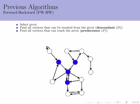
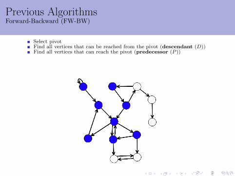
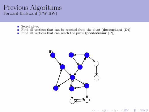
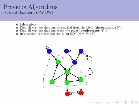
Previous AlgorithmsForward-Backward (FW-BW)
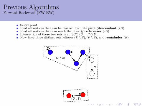
Select pivotFind all vertices that can be reached from the pivot (descendant (D))Find all vertices that can reach the pivot (predecessor (P ))Intersection of those two sets is an SCC (S = P ∩D)Now have three distinct sets leftover (D \ S), (P \ S), and remainder (R)
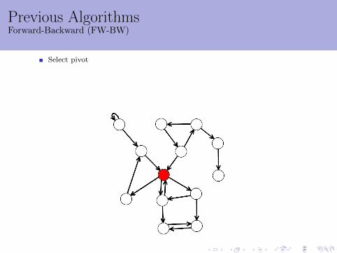
Previous AlgorithmsForward-Backward (FW-BW)
Select pivot
Find all vertices that can be reached from the pivot (descendant (D))Find all vertices that can reach the pivot (predecessor (P ))Intersection of those two sets is an SCC (S = P ∩D)Now have three distinct sets leftover (D \ S), (P \ S), and remainder (R)
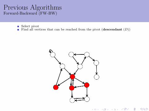
Previous AlgorithmsForward-Backward (FW-BW)
Select pivotFind all vertices that can be reached from the pivot (descendant (D))
Find all vertices that can reach the pivot (predecessor (P ))Intersection of those two sets is an SCC (S = P ∩D)Now have three distinct sets leftover (D \ S), (P \ S), and remainder (R)
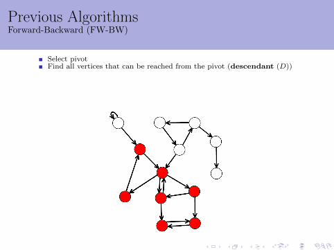
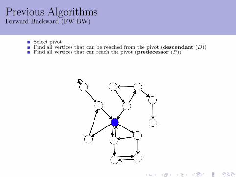
Previous AlgorithmsForward-Backward (FW-BW)
Select pivotFind all vertices that can be reached from the pivot (descendant (D))Find all vertices that can reach the pivot (predecessor (P ))
Intersection of those two sets is an SCC (S = P ∩D)Now have three distinct sets leftover (D \ S), (P \ S), and remainder (R)
Previous AlgorithmsForward-Backward (FW-BW)
Select pivotFind all vertices that can be reached from the pivot (descendant (D))Find all vertices that can reach the pivot (predecessor (P ))Intersection of those two sets is an SCC (S = P ∩D)
Now have three distinct sets leftover (D \ S), (P \ S), and remainder (R)
Previous AlgorithmsForward-Backward (FW-BW)
Select pivotFind all vertices that can be reached from the pivot (descendant (D))Find all vertices that can reach the pivot (predecessor (P ))Intersection of those two sets is an SCC (S = P ∩D)Now have three distinct sets leftover (D \ S), (P \ S), and remainder (R)
Forward-Backward (FW-BW) Algorithm
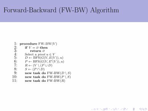
1: procedure FW-BW(V )2: if V = ∅ then3: return ∅4: Select a pivot u ∈ V5: D ← BFS(G(V,E(V )), u)6: P ← BFS(G(V,E′(V )), u)7: R← (V \ (P ∪D)8: S ← (P ∩D)9: new task do FW-BW(D \ S)
10: new task do FW-BW(P \ S)11: new task do FW-BW(R)
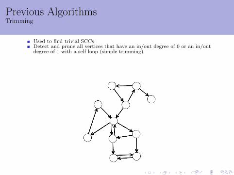
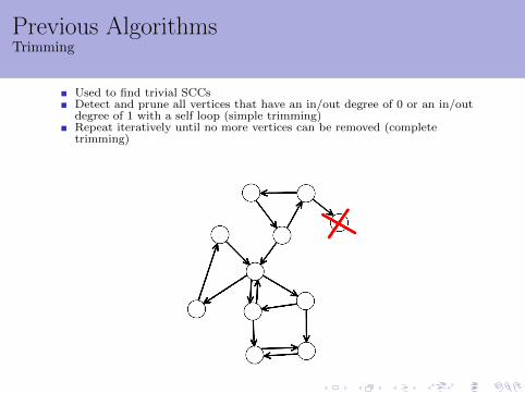
Previous AlgorithmsTrimming
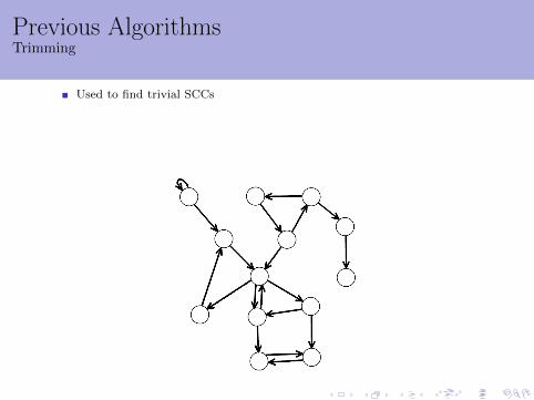
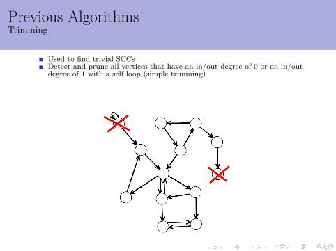
Used to find trivial SCCs
Detect and prune all vertices that have an in/out degree of 0 or an in/outdegree of 1 with a self loop (simple trimming)Repeat iteratively until no more vertices can be removed (completetrimming)
Previous AlgorithmsTrimming
Used to find trivial SCCsDetect and prune all vertices that have an in/out degree of 0 or an in/outdegree of 1 with a self loop (simple trimming)
Repeat iteratively until no more vertices can be removed (completetrimming)
Previous AlgorithmsTrimming
Used to find trivial SCCsDetect and prune all vertices that have an in/out degree of 0 or an in/outdegree of 1 with a self loop (simple trimming)
Repeat iteratively until no more vertices can be removed (completetrimming)
Previous AlgorithmsTrimming
Used to find trivial SCCsDetect and prune all vertices that have an in/out degree of 0 or an in/outdegree of 1 with a self loop (simple trimming)Repeat iteratively until no more vertices can be removed (completetrimming)

Previous AlgorithmsTrimming
Used to find trivial SCCsDetect and prune all vertices that have an in/out degree of 0 or an in/outdegree of 1 with a self loop (simple trimming)Repeat iteratively until no more vertices can be removed (completetrimming)
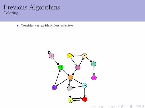
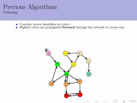
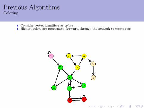
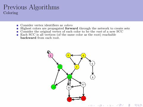
Previous AlgorithmsColoring
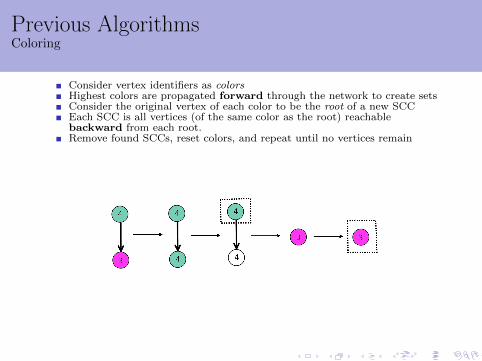
Consider vertex identifiers as colors
Highest colors are propagated forward through the network to create setsConsider the original vertex of each color to be the root of a new SCCEach SCC is all vertices (of the same color as the root) reachablebackward from each root.Remove found SCCs, reset colors, and repeat until no vertices remain
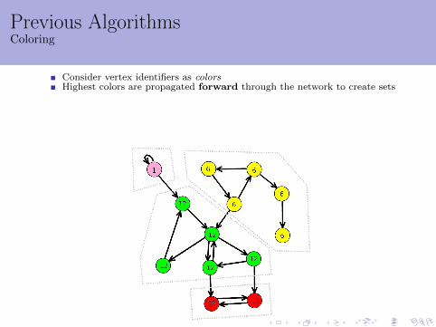
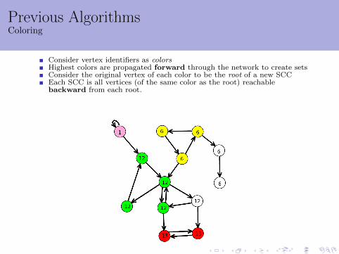
Previous AlgorithmsColoring
Consider vertex identifiers as colorsHighest colors are propagated forward through the network to create sets
Consider the original vertex of each color to be the root of a new SCCEach SCC is all vertices (of the same color as the root) reachablebackward from each root.Remove found SCCs, reset colors, and repeat until no vertices remain
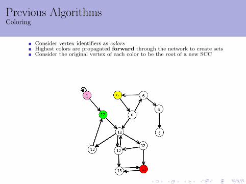
Previous AlgorithmsColoring
Consider vertex identifiers as colorsHighest colors are propagated forward through the network to create setsConsider the original vertex of each color to be the root of a new SCC
Each SCC is all vertices (of the same color as the root) reachablebackward from each root.Remove found SCCs, reset colors, and repeat until no vertices remain
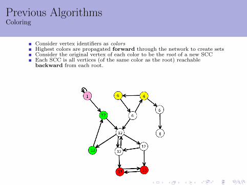
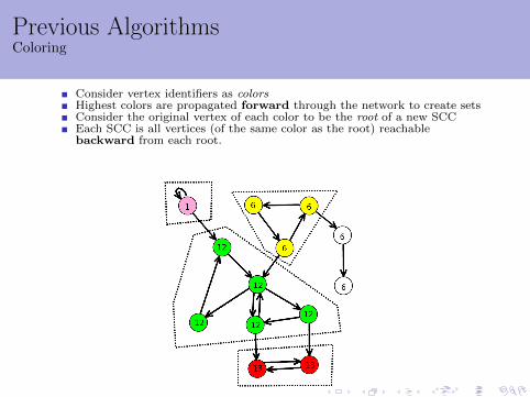
Previous AlgorithmsColoring
Consider vertex identifiers as colorsHighest colors are propagated forward through the network to create setsConsider the original vertex of each color to be the root of a new SCCEach SCC is all vertices (of the same color as the root) reachablebackward from each root.
Remove found SCCs, reset colors, and repeat until no vertices remain
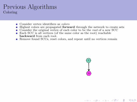
Previous AlgorithmsColoring
Consider vertex identifiers as colorsHighest colors are propagated forward through the network to create setsConsider the original vertex of each color to be the root of a new SCCEach SCC is all vertices (of the same color as the root) reachablebackward from each root.Remove found SCCs, reset colors, and repeat until no vertices remain
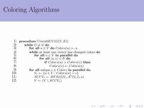
Coloring Algorithms
1: procedure ColorSCC(G(V,E))2: while G 6= ∅ do3: for all u ∈ V do Colors(u)← u
4: while at least one vertex has changed colors do5: for all u ∈ V in parallel do6: for all 〈u, v〉 ∈ E do7: if Colors(u) > Colors(v) then8: Colors(v)← Colors(u)
9: for all unique c ∈ Colors in parallel do10: Vc ← {u ∈ V : Colors(u) = c}11: SCCVc ← BFS(G(Vc, E′(Vc)), u)12: V ← (V \ SCCVc)
Today’s Biz
1. Quick Review
2. Reminders
3. Parallel SCC
4. More Centrality
5. Even More MPI
6. More PageRank Tutorial
9 / 16

Network CentralitySlides from Ahmed Louri, University of Arizona
10 / 16
Network Centrality
Based on materials by Lada Adamic, UMichigan
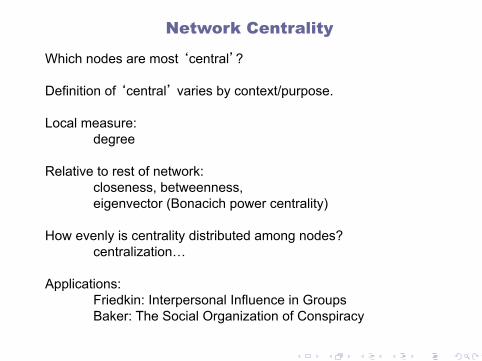
Which nodes are most ‘central’? Definition of ‘central’ varies by context/purpose. Local measure:
degree Relative to rest of network:
closeness, betweenness, eigenvector (Bonacich power centrality)
How evenly is centrality distributed among nodes?
centralization… Applications:
Friedkin: Interpersonal Influence in Groups Baker: The Social Organization of Conspiracy
Network Centrality

Centrality: Who’s Important Based On Their Network Position
Y
X
Y
X
Y X
Y
X
indegree
In each of the following networks, X has higher centrality than Y according to a particular measure
outdegree betweenness closeness
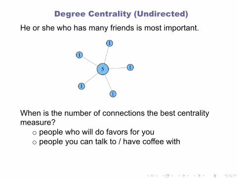
He or she who has many friends is most important.
Degree Centrality (Undirected)
When is the number of connections the best centrality measure?
o people who will do favors for you o people you can talk to / have coffee with
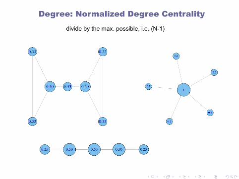
Degree: Normalized Degree Centrality
divide by the max. possible, i.e. (N-1)

Freeman’s general formula for centralization (can use other metrics, e.g. gini coefficient or standard deviation):
€
CD =CD (n
*) −CD (i)[ ]i=1
g∑[(N −1)(N − 2)]
Centralization: How Equal Are The Nodes?
How much variation is there in the centrality scores among the nodes?
maximum value in the network
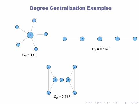
Degree Centralization Examples
CD = 0.167
CD = 0.167
CD = 1.0

Degree Centralization Examples
example financial trading networks
high centralization: one node trading with many others
low centralization: trades are more evenly distributed
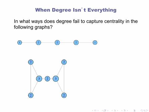
When Degree Isn’t Everything
In what ways does degree fail to capture centrality in the following graphs?
In What Contexts May Degree Be Insufficient To Describe Centrality?
n ability to broker between groups n likelihood that information originating anywhere in the
network reaches you…
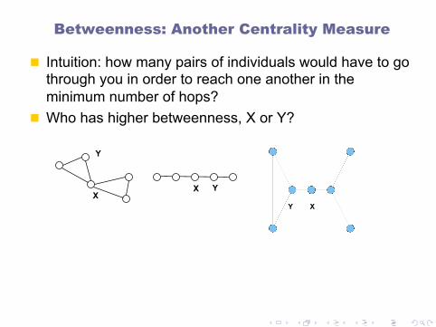
Betweenness: Another Centrality Measure
n Intuition: how many pairs of individuals would have to go through you in order to reach one another in the minimum number of hops?
n Who has higher betweenness, X or Y?
Y X
Y
X
X Y
€
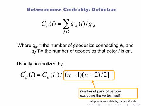
CB (i) = g jk (i) /g jkj<k∑
Where gjk = the number of geodesics connecting jk, and gjk(i)= the number of geodesics that actor i is on.
Usually normalized by:
€
CB' (i) = CB (i ) /[(n −1)(n − 2) /2]
number of pairs of vertices excluding the vertex itself
Betweenness Centrality: Definition
adapted from a slide by James Moody
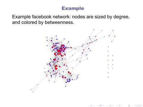
Example facebook network: nodes are sized by degree, and colored by betweenness.
Example
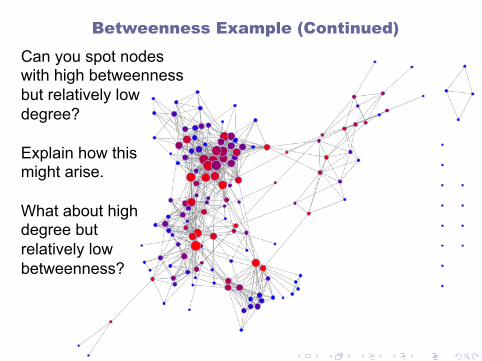
Can you spot nodes with high betweenness but relatively low degree? Explain how this might arise.
Betweenness Example (Continued)
What about high degree but relatively low betweenness?
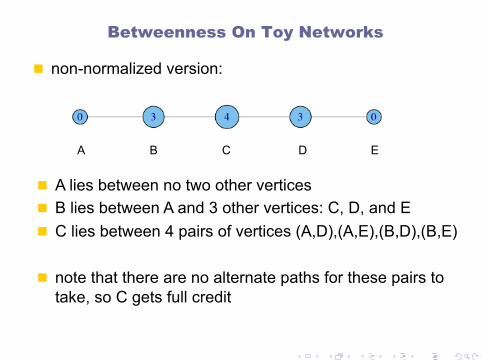
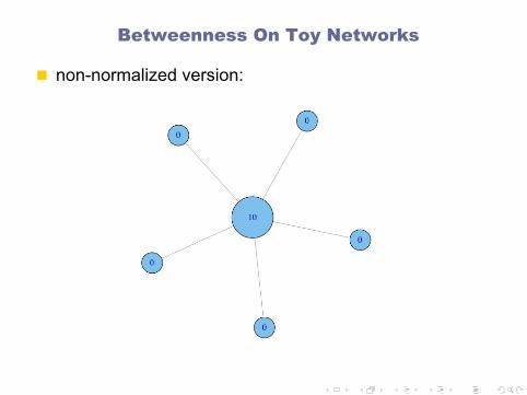
Betweenness On Toy Networks
n non-normalized version:
A B C E D
n A lies between no two other vertices n B lies between A and 3 other vertices: C, D, and E n C lies between 4 pairs of vertices (A,D),(A,E),(B,D),(B,E)
n note that there are no alternate paths for these pairs to take, so C gets full credit
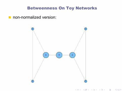
Betweenness On Toy Networks
n non-normalized version:
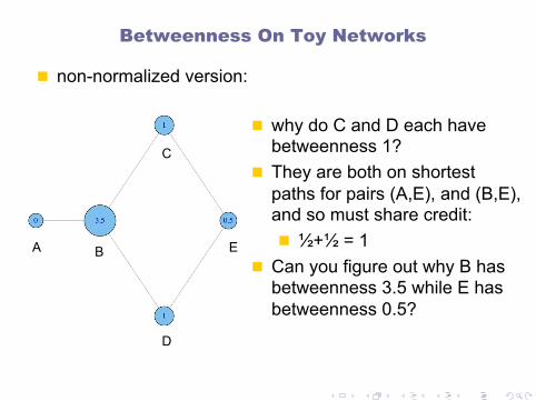
Betweenness On Toy Networks
n non-normalized version:
Betweenness On Toy Networks
n non-normalized version:
A B
C
E
D
n why do C and D each have betweenness 1?
n They are both on shortest paths for pairs (A,E), and (B,E), and so must share credit: n ½+½ = 1
n Can you figure out why B has betweenness 3.5 while E has betweenness 0.5?
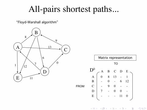
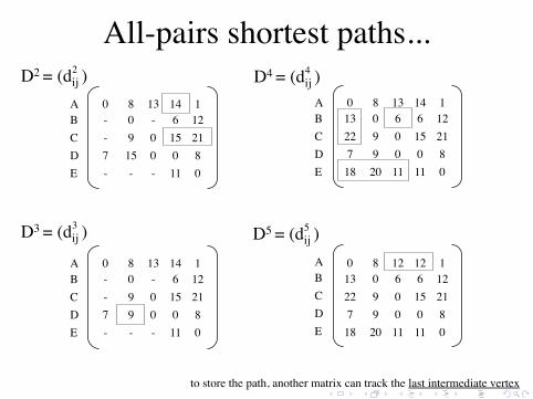
All-pairs shortest paths... “Floyd-Warshall algorithm”!
A
B
E D
C
8
13
1
6
12
9
7 0
11 0 8 13 - 1 - 0 - 6 12 - 9 0 - - 7 - 0 0 - - - - 11 0
ABCDE
FROM
TO
Matrix representation!
D0 A B C D E
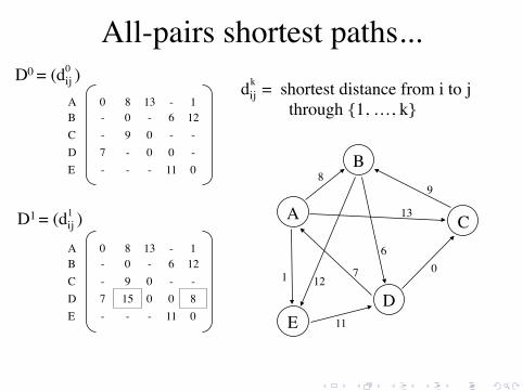
All-pairs shortest paths...
0 8 13 - 1 - 0 - 6 12 - 9 0 - - 7 - 0 0 - - - - 11 0
ABCDE
D0 = (dij ) 0
D1 = (dij ) 1
dij = shortest distance from i to j through {1, …, k}
k
0 8 13 - 1 - 0 - 6 12 - 9 0 - - 7 15 0 0 8 - - - 11 0
ABCDE
A
B
E D
C
8
13
1
6
12
9
7 0
11
All-pairs shortest paths...
0 8 13 14 1 - 0 - 6 12 - 9 0 15 21 7 15 0 0 8 - - - 11 0
ABCDE
D2 = (dij ) 2
0 8 13 14 1 - 0 - 6 12 - 9 0 15 21 7 9 0 0 8 - - - 11 0
ABCDE
D3 = (dij ) 3
0 8 13 14 1 13 0 6 6 12 22 9 0 15 21 7 9 0 0 8 18 20 11 11 0
ABCDE
D4 = (dij ) 4
ABCDE
D5 = (dij ) 5
to store the path, another matrix can track the last intermediate vertex
0 8 12 12 1 13 0 6 6 12 22 9 0 15 21 7 9 0 0 8 18 20 11 11 0
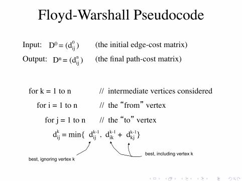
Floyd-Warshall Pseudocode
Input: (the initial edge-cost matrix)
Output: (the final path-cost matrix) D0 = (dij )
0
Dn = (dij ) n
for k = 1 to n // intermediate vertices considered
for i = 1 to n // the “from” vertex
for j = 1 to n // the “to” vertex
dij = min{ dij , dik + dkj } k-1 k k-1 k-1
best, ignoring vertex k best, including vertex k
Closeness: Another Centrality Measure
n What if it’s not so important to have many direct friends? n Or be “between” others n But one still wants to be in the “middle” of things, not too
far from the center
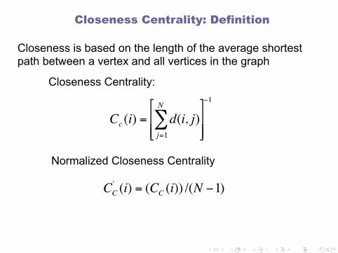
Closeness is based on the length of the average shortest path between a vertex and all vertices in the graph
€
Cc (i) = d(i, j)j=1
N
∑#
$ % %
&
' ( (
−1
€
CC' (i) = (CC (i)) /(N −1)
Closeness Centrality:
Normalized Closeness Centrality
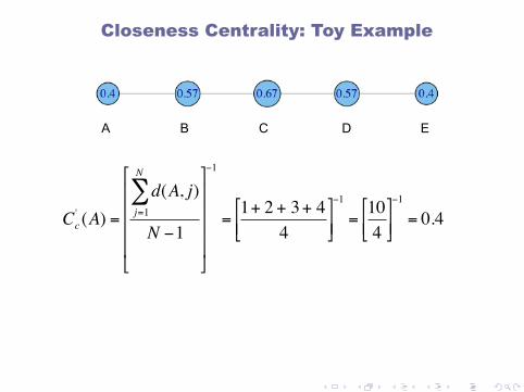
Closeness Centrality: Definition
€
Cc' (A) =
d(A, j)j=1
N
∑
N −1
$
%
& & & &
'
(
) ) ) )
−1
=1+ 2 + 3+ 4
4$
% & '
( )
−1
=104
$
% & '
( )
−1
= 0.4
Closeness Centrality: Toy Example
A B C E D
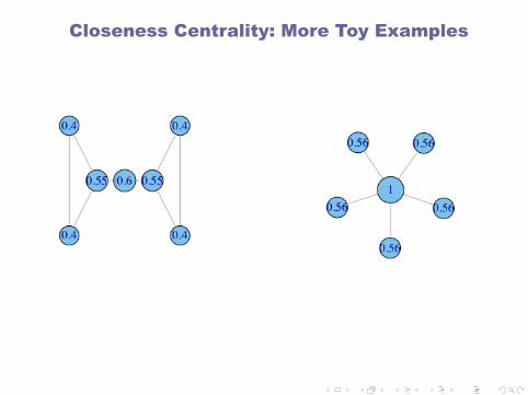
Closeness Centrality: More Toy Examples
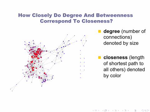
n degree (number of connections) denoted by size
n closeness (length of shortest path to all others) denoted by color
How Closely Do Degree And Betweenness Correspond To Closeness?
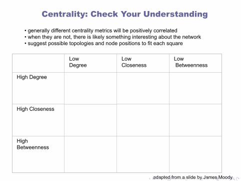
• generally different centrality metrics will be positively correlated • when they are not, there is likely something interesting about the network • suggest possible topologies and node positions to fit each square
Low Degree Low
Closeness Low Betweenness
High Degree
High Closeness
High Betweenness
Centrality: Check Your Understanding
adapted from a slide by James Moody
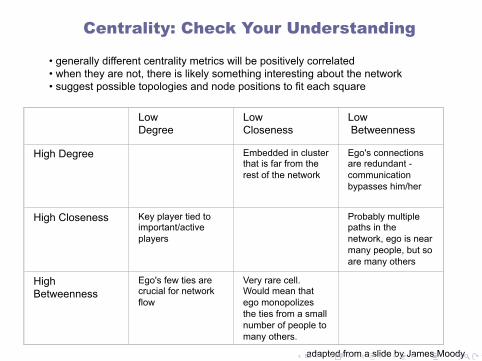
• generally different centrality metrics will be positively correlated • when they are not, there is likely something interesting about the network • suggest possible topologies and node positions to fit each square
Centrality: Check Your Understanding
adapted from a slide by James Moody
High Degree
Embedded in cluster that is far from the rest of the network
Ego's connections are redundant - communication bypasses him/her
High Closeness
Key player tied to important/active players
Probably multiple paths in the network, ego is near many people, but so are many others
High Betweenness
Ego's few ties are crucial for network flow
Very rare cell. Would mean that ego monopolizes the ties from a small number of people to many others.
Low Degree Low
Closeness Low Betweenness
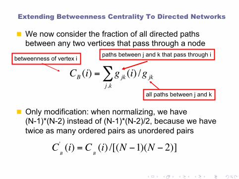
Extending Betweenness Centrality To Directed Networks
n We now consider the fraction of all directed paths between any two vertices that pass through a node
n Only modification: when normalizing, we have (N-1)*(N-2) instead of (N-1)*(N-2)/2, because we have twice as many ordered pairs as unordered pairs €
CB (i) = g jkj ,k∑ (i) /g jk
betweenness of vertex i paths between j and k that pass through i
all paths between j and k
€
CB
' (i) = CB(i) /[(N −1)(N − 2)]
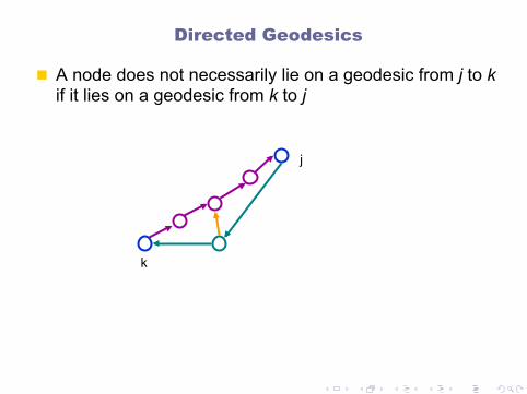
Directed Geodesics
n A node does not necessarily lie on a geodesic from j to k if it lies on a geodesic from k to j
k
j
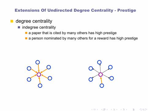
Extensions Of Undirected Degree Centrality - Prestige
n degree centrality n indegree centrality
n a paper that is cited by many others has high prestige n a person nominated by many others for a reward has high prestige
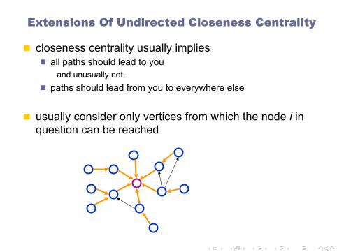
Extensions Of Undirected Closeness Centrality
n closeness centrality usually implies n all paths should lead to you
and unusually not: n paths should lead from you to everywhere else
n usually consider only vertices from which the node i in question can be reached
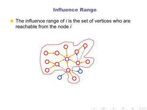
Influence Range
n The influence range of i is the set of vertices who are reachable from the node i
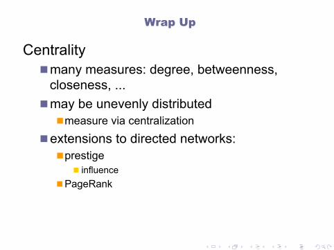
Wrap Up
Centrality n many measures: degree, betweenness,
closeness, ... n may be unevenly distributed
n measure via centralization
n extensions to directed networks: n prestige
n influence n PageRank

Today’s Biz
1. Quick Review
2. Reminders
3. Parallel SCC
4. More Centrality
5. Even More MPI
6. More PageRank Tutorial
11 / 16

Even More MPI – AlltoallvSlides from Lori Pollock, University of Delaware
12 / 16

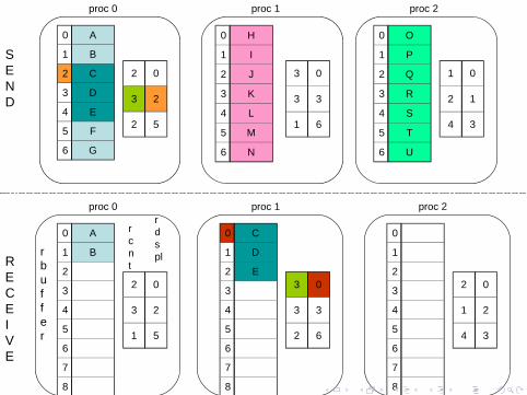
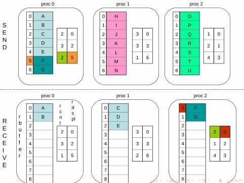
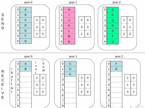
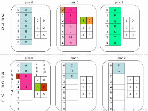
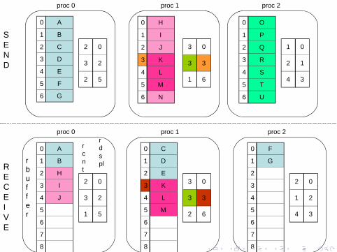
MPI_AlltoAllv Function Outlineint MPI_Alltoallv ( void *sendbuf, int *sendcnts, int *sdispls, MPI_Datatype sendtype, void *recvbuf, int *recvcnts, int *rdispls, MPI_Datatype recvtype, MPI_Comm comm )
Input Parameterssendbuf starting address of send buffer (choice) sendcounts integer array equal to the group size specifying the number of elements to send to each processor sdispls integer array (of length group size). Entry j specifies the displacement (relative to sendbuf from which to take the outgoing data destined for process j recvcounts integer array equal to the group size specifying the maximum number of elements that can be received from each processor rdispls integer array (of length group size). Entry i specifies the displacement (relative to recvbuf at which to place the incoming data from process i

2 0
3 2
2 5
0 A
1 B
2 C
3 D
4 E
5 F
6 G
0 H
1 I
2 J
3 K
4 L
5 M
6 N
0 O
1 P
2 Q
3 R
4 S
5 T
6 U
3 0
3 3
1 6
1 0
2 1
4 3
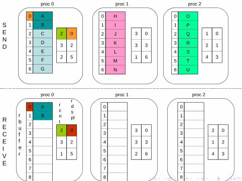
proc 0 proc 1 proc 2
send buffersend count array
send displacement array
Each node in parallel community has
0 2
1 3
2 2
0 A
1 B
2 C
3 D
4 E
5 F
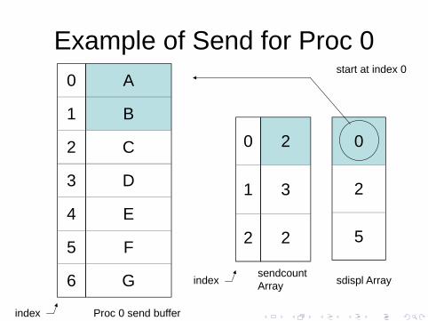
6 G
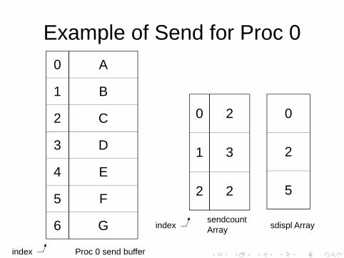
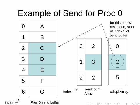
Example of Send for Proc 0
Proc 0 send buffer
sendcount Array
0
2
5
sdispl Array
index
index
0 2
1 3
2 2
0 A
1 B
2 C
3 D
4 E
5 F
6 G
Example of Send for Proc 0
Proc 0 send buffer
sendcount Array
0
2
5
sdispl Array
index
index
start at index 0
0 2
1 3
2 2
0 A
1 B
2 C
3 D
4 E
5 F
6 G
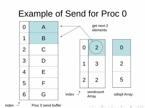
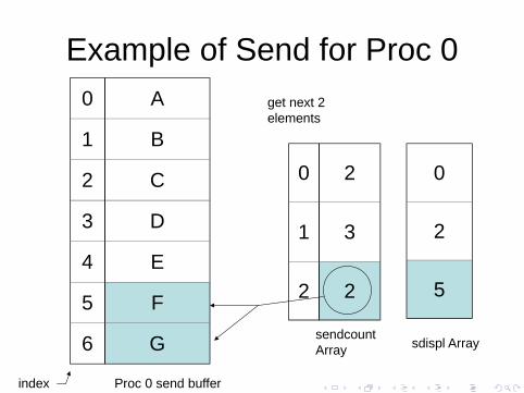
Example of Send for Proc 0
Proc 0 send buffer
sendcount Array
0
2
5
sdispl Array
index
index
get next 2 elements
0 2
1 3
2 2
0 A
1 B
2 C
3 D
4 E
5 F
6 G
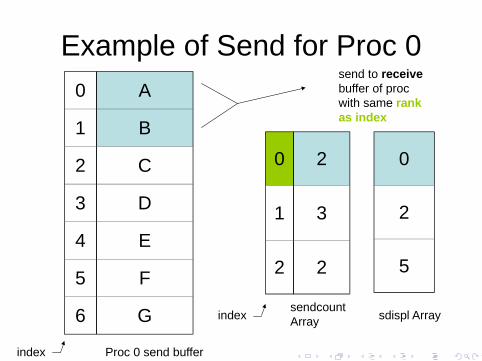
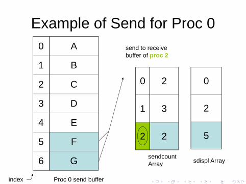
Example of Send for Proc 0
Proc 0 send buffer
sendcount Array
0
2
5
sdispl Array
index
index
send to receive buffer of proc with same rank as index
0 2
1 3
2 2
0 A
1 B
2 C
3 D
4 E
5 F
6 G
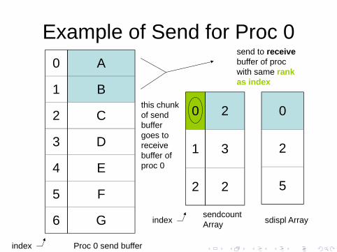
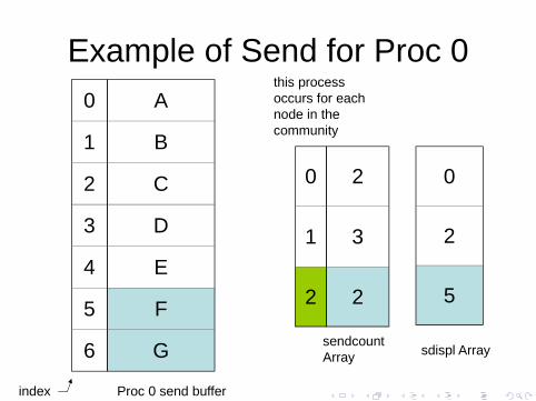
Example of Send for Proc 0
Proc 0 send buffer
sendcount Array
0
2
5
sdispl Array
index
index
send to receive buffer of proc with same rank as index
this chunk of send buffer goes to receive buffer of proc 0
0 2
1 3
2 2
0 A
1 B
2 C
3 D
4 E
5 F
6 G
Example of Send for Proc 0
Proc 0 send buffer
sendcount Array
0
2
5
sdispl Array
index
index
for this proc’s next send, start at index 2 of send buffer
0 2
1 3
2 2
0 A
1 B
2 C
3 D
4 E
5 F
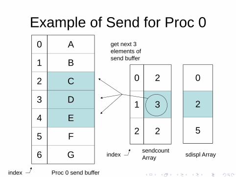
6 G
Example of Send for Proc 0
Proc 0 send buffer
sendcount Array
0
2
5
sdispl Array
index
index
get next 3 elements of send buffer
0 2
1 3
2 2
0 A
1 B
2 C
3 D
4 E
5 F
6 G
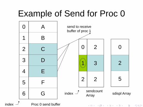
Example of Send for Proc 0
Proc 0 send buffer
sendcount Array
0
2
5
sdispl Array
index
index
send to receive buffer of proc 1
0 2
1 3
2 2
0 A
1 B
2 C
3 D
4 E
5 F
6 G
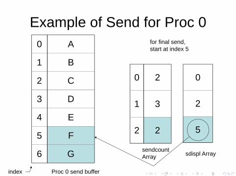
Example of Send for Proc 0
Proc 0 send buffer
sendcount Array
0
2
5
sdispl Array
index
for final send, start at index 5
0 2
1 3
2 2
0 A
1 B
2 C
3 D
4 E
5 F
6 G
Example of Send for Proc 0
Proc 0 send buffer
sendcount Array
0
2
5
sdispl Array
index
get next 2 elements
0 2
1 3
2 2
0 A
1 B
2 C
3 D
4 E
5 F
6 G
Example of Send for Proc 0
Proc 0 send buffer
sendcount Array
0
2
5
sdispl Array
index
send to receive buffer of proc 2
0 2
1 3
2 2
0 A
1 B
2 C
3 D
4 E
5 F
6 G
Example of Send for Proc 0
Proc 0 send buffer
sendcount Array
0
2
5
sdispl Array
index
this process occurs for each node in the community

2 0
3 2
2 5
0 A
1 B
2 C
3 D
4 E
5 F
6 G
0 H
1 I
2 J
3 K
4 L
5 M
6 N
0 O
1 P
2 Q
3 R
4 S
5 T
6 U
3 0
3 3
1 6
1 0
2 1
4 3
proc 0 proc 1 proc 2
2 0
3 2
1 5
0
1
2
3
4
5
6
7
8
proc 0
3 0
3 3
2 6
0
1
2
3
4
5
6
7
8
proc 1
2 0
1 2
4 3
0
1
2
3
4
5
6
7
8
proc 2
SEND
RECE I VE
rcnt
rdsplr
buf fer
2 0
3 2
2 5
0 A
1 B
2 C
3 D
4 E
5 F
6 G
0 H
1 I
2 J
3 K
4 L
5 M
6 N
0 O
1 P
2 Q
3 R
4 S
5 T
6 U
3 0
3 3
1 6
1 0
2 1
4 3
proc 0 proc 1 proc 2
2 0
3 2
1 5
0 A
1 B
2
3
4
5
6
7
8
proc 0
3 0
3 3
2 6
0
1
2
3
4
5
6
7
8
proc 1
2 0
1 2
4 3
0
1
2
3
4
5
6
7
8
proc 2
SEND
RECE I VE
rcnt
rdsplr
buf fer
2 0
3 2
2 5
0 A
1 B
2 C
3 D
4 E
5 F
6 G
0 H
1 I
2 J
3 K
4 L
5 M
6 N
0 O
1 P
2 Q
3 R
4 S
5 T
6 U
3 0
3 3
1 6
1 0
2 1
4 3
proc 0 proc 1 proc 2
2 0
3 2
1 5
0 A
1 B
2
3
4
5
6
7
8
proc 0
3 0
3 3
2 6
0 C
1 D
2 E
3
4
5
6
7
8
proc 1
2 0
1 2
4 3
0
1
2
3
4
5
6
7
8
proc 2
SEND
RECE I VE
rcnt
rdsplr
buf fer
2 0
3 2
2 5
0 A
1 B
2 C
3 D
4 E
5 F
6 G
0 H
1 I
2 J
3 K
4 L
5 M
6 N
0 O
1 P
2 Q
3 R
4 S
5 T
6 U
3 0
3 3
1 6
1 0
2 1
4 3
proc 0 proc 1 proc 2
2 0
3 2
1 5
0 A
1 B
2
3
4
5
6
7
8
proc 0
3 0
3 3
2 6
0 C
1 D
2 E
3
4
5
6
7
8
proc 1
2 0
1 2
4 3
0 F
1 G
2
3
4
5
6
7
8
proc 2
SEND
RECE I VE
rcnt
rdsplr
buf fer
2 0
3 2
2 5
0 A
1 B
2 C
3 D
4 E
5 F
6 G
0 H
1 I
2 J
3 K
4 L
5 M
6 N
0 O
1 P
2 Q
3 R
4 S
5 T
6 U
3 0
3 3
1 6
1 0
2 1
4 3
proc 0 proc 1 proc 2
2 0
3 2
1 5
0 A
1 B
2 H
3 I
4 J
5
6
7
8
proc 0
3 0
3 3
2 6
0 C
1 D
2 E
3 K
4 L
5 M
6
7
8
proc 1
2 0
1 2
4 3
0 F
1 G
2 N
3
4
5
6
7
8
proc 2
SEND
RECE I VE
rcnt
rdsplr
buf fer
2 0
3 2
2 5
0 A
1 B
2 C
3 D
4 E
5 F
6 G
0 H
1 I
2 J
3 K
4 L
5 M
6 N
0 O
1 P
2 Q
3 R
4 S
5 T
6 U
3 0
3 3
1 6
1 0
2 1
4 3
proc 0 proc 1 proc 2
2 0
3 2
1 5
0 A
1 B
2 H
3 I
4 J
5 O
6
7
8
proc 0
3 0
3 3
2 6
0 C
1 D
2 E
3 K
4 L
5 M
6
7
8
proc 1
2 0
1 2
4 3
0 F
1 G
2 N
3
4
5
6
7
8
proc 2
SEND
RECE I VE
rcnt
rdsplr
buf fer

2 0
3 2
2 5
0 A
1 B
2 C
3 D
4 E
5 F
6 G
0 H
1 I
2 J
3 K
4 L
5 M
6 N
0 O
1 P
2 Q
3 R
4 S
5 T
6 U
3 0
3 3
1 6
1 0
2 1
4 3
proc 0 proc 1 proc 2
2 0
3 2
1 5
0 A
1 B
2 H
3 I
4 J
5 O
6
7
8
proc 0
3 0
3 3
2 6
0 C
1 D
2 E
3 K
4 L
5 M
6 P
7 Q
8
proc 1
2 0
1 2
4 3
0 F
1 G
2 N
3
4
5
6
7
8
proc 2
SEND
RECE I VE
rcnt
rdsplr
buf fer
2 0
3 2
2 5
0 A
1 B
2 C
3 D
4 E
5 F
6 G
0 H
1 I
2 J
3 K
4 L
5 M
6 N
0 O
1 P
2 Q
3 R
4 S
5 T
6 U
3 0
3 3
1 6
1 0
2 1
4 3
proc 0 proc 1 proc 2
2 0
3 2
1 5
0 A
1 B
2 H
3 I
4 J
5 O
6
7
8
proc 0
3 0
3 3
2 6
0 C
1 D
2 E
3 K
4 L
5 M
6 P
7 Q
8
proc 1
2 0
1 2
4 3
0 F
1 G
2 N
3 R
4 S
5 T
6 U
7
8
proc 2
SEND
RECE I VE
rcnt
rdsplr
buf fer
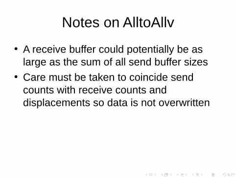
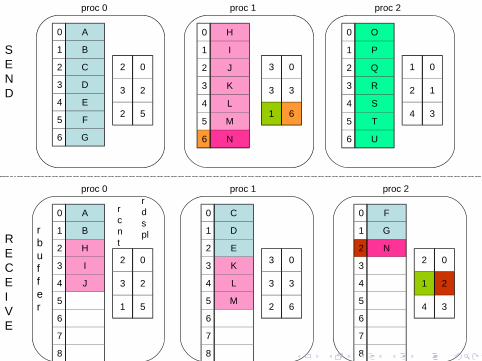
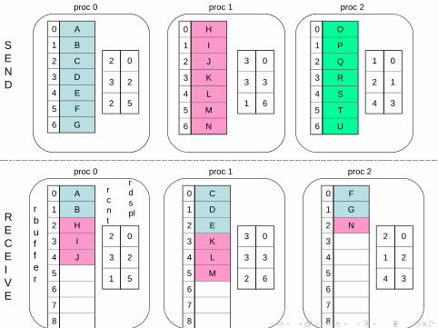
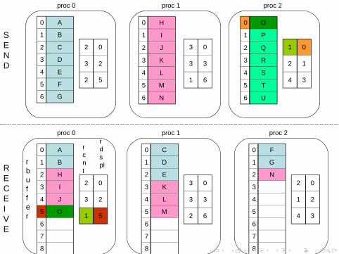
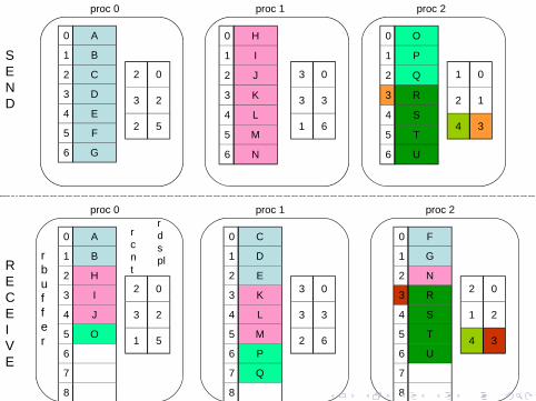
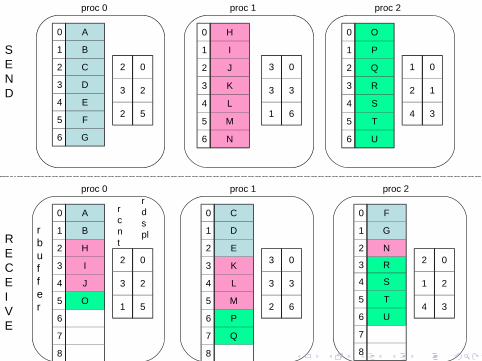
Notes on AlltoAllv
• A receive buffer could potentially be as large as the sum of all send buffer sizes
• Care must be taken to coincide send counts with receive counts and displacements so data is not overwritten

Today’s Biz
1. Quick Review
2. Reminders
3. Parallel SCC
4. More Centrality
5. Even More MPI
6. More PageRank Tutorial
13 / 16
More PageRank Tutorial
1. OpenMP - Work Queueing
2. MPI - Alltoallv Communication
14 / 16

More PageRank TutorialBlank code and data available on website
(Lecture 5)www.cs.rpi.edu/∼slotag/classes/FA16/index.html
15 / 16